
A Dynamic Investigation of a Solar Absorption Plant with Nanofluids for Air-Conditioning of an Office Building in a Mild Climate Zone

 ,
,  ,
,  ,
,  ,
,
Abstract
1. Introduction
- Exclusive use of nanofluids in the solar loop with detailed thermo-physical modeling.
- Dynamic, hourly simulation in TRNSYS over the summer period.
- Sensitivity analysis on flow rate and concentration effects.
- Assessment of pumping energy penalty, often overlooked in the literature.
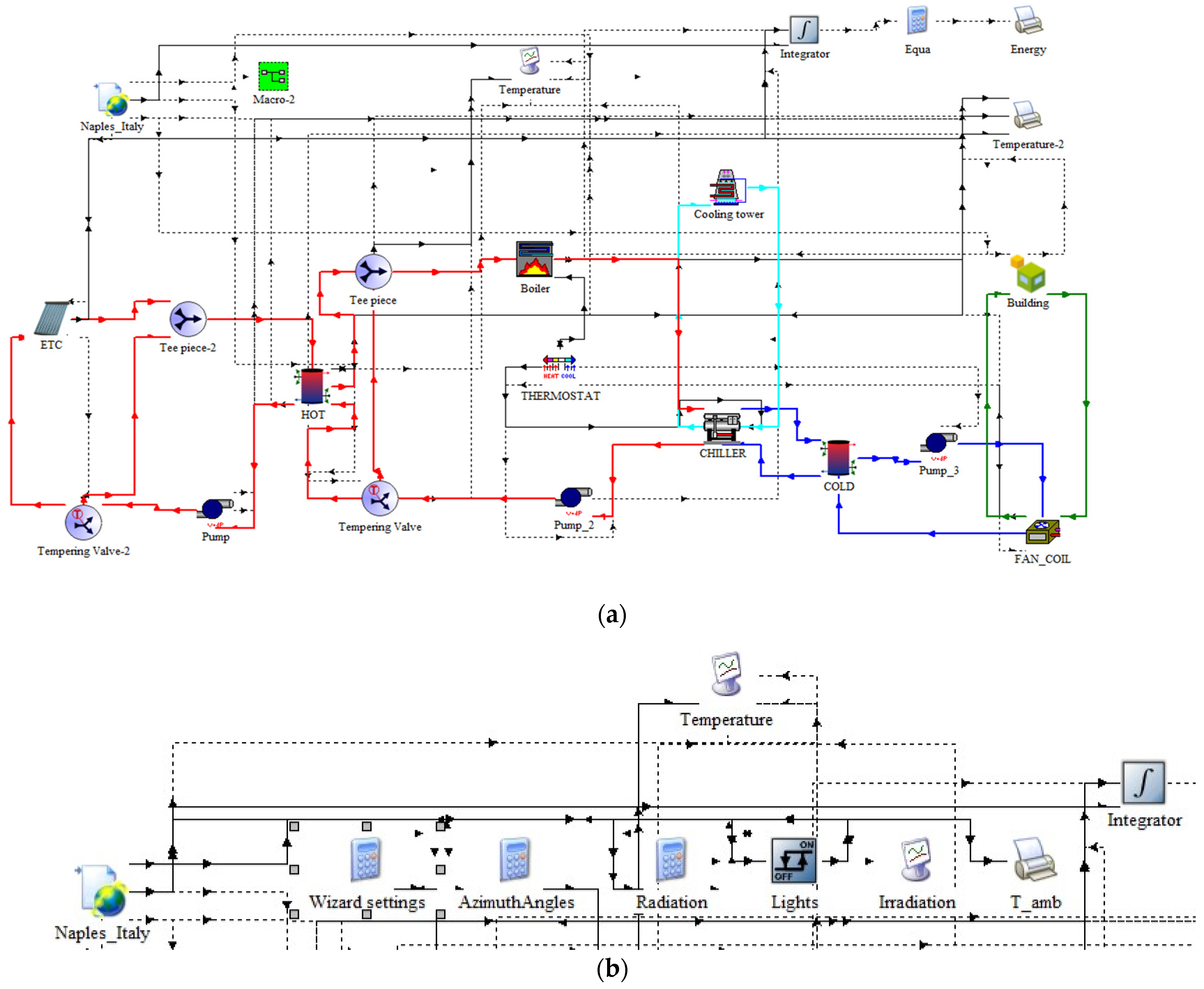
2. System Configuration
3. Modeling in TRNSYS
- The simulation does not take into account the outcomes of the boiling of the auxiliary fluid;
- The analysis does not take into account the decreases in pressure that arise within the pipes and valves. Therefore, the predicted performance values may be higher than those in a real system.
3.1. Solar Collector
3.2. Storage Tank
3.3. Absorption Chiller
3.4. Building Loads
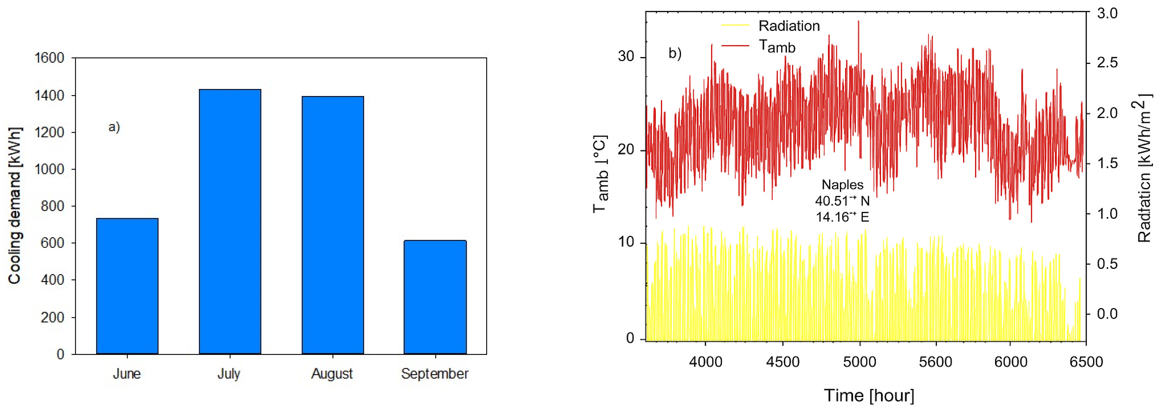
3.5. Weather Data
3.6. Uncertainty Analysis
4. Performance Factors
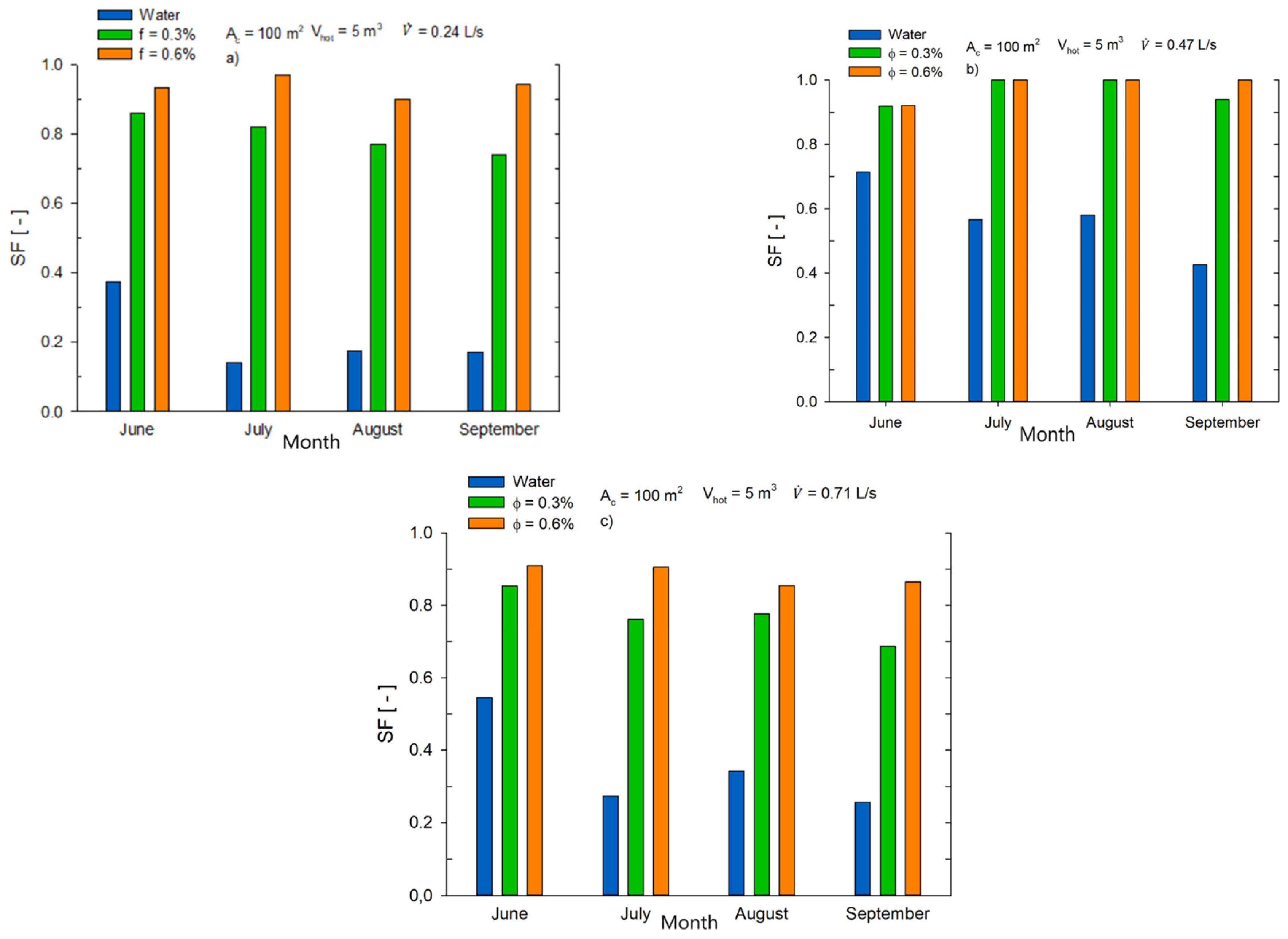
4.1. Solar Fraction
4.2. Primary Energy Savings
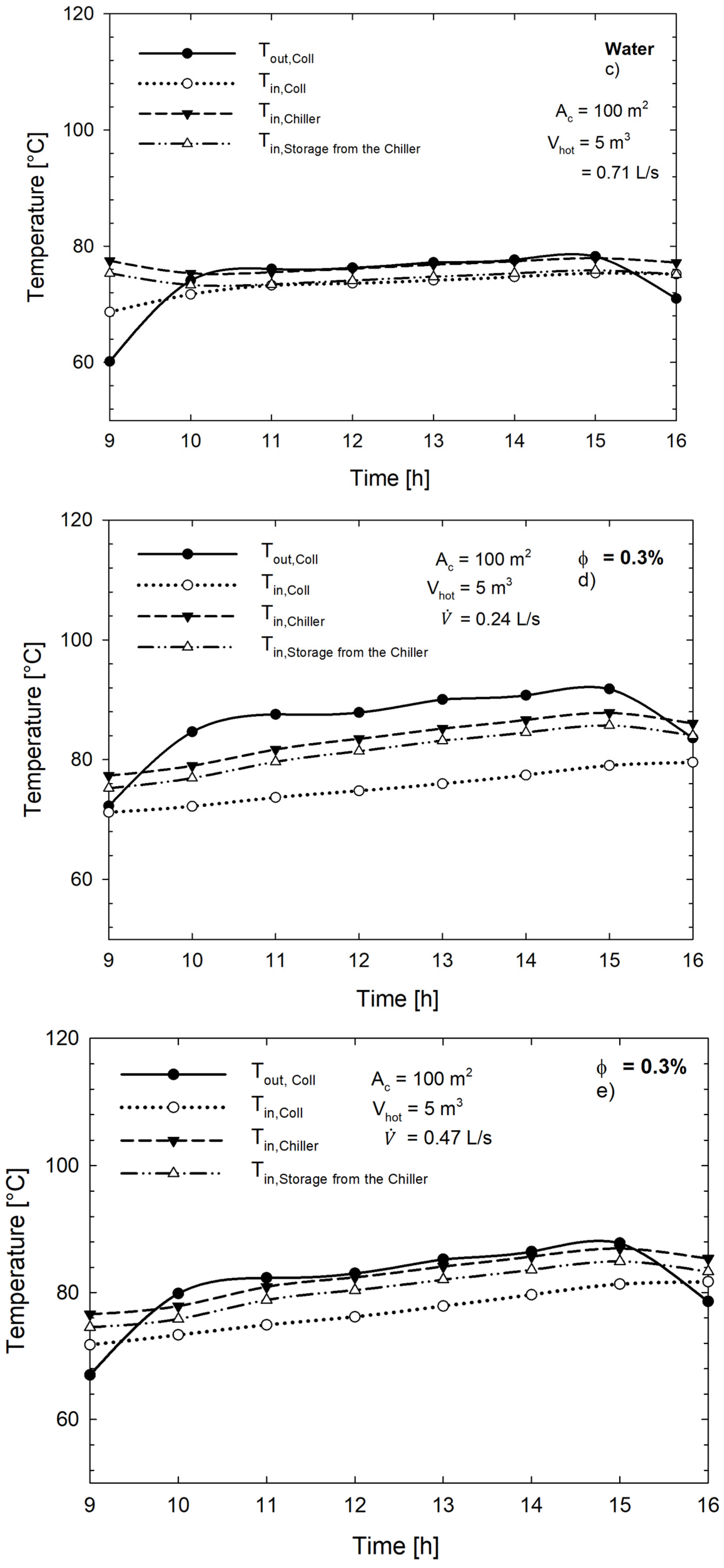
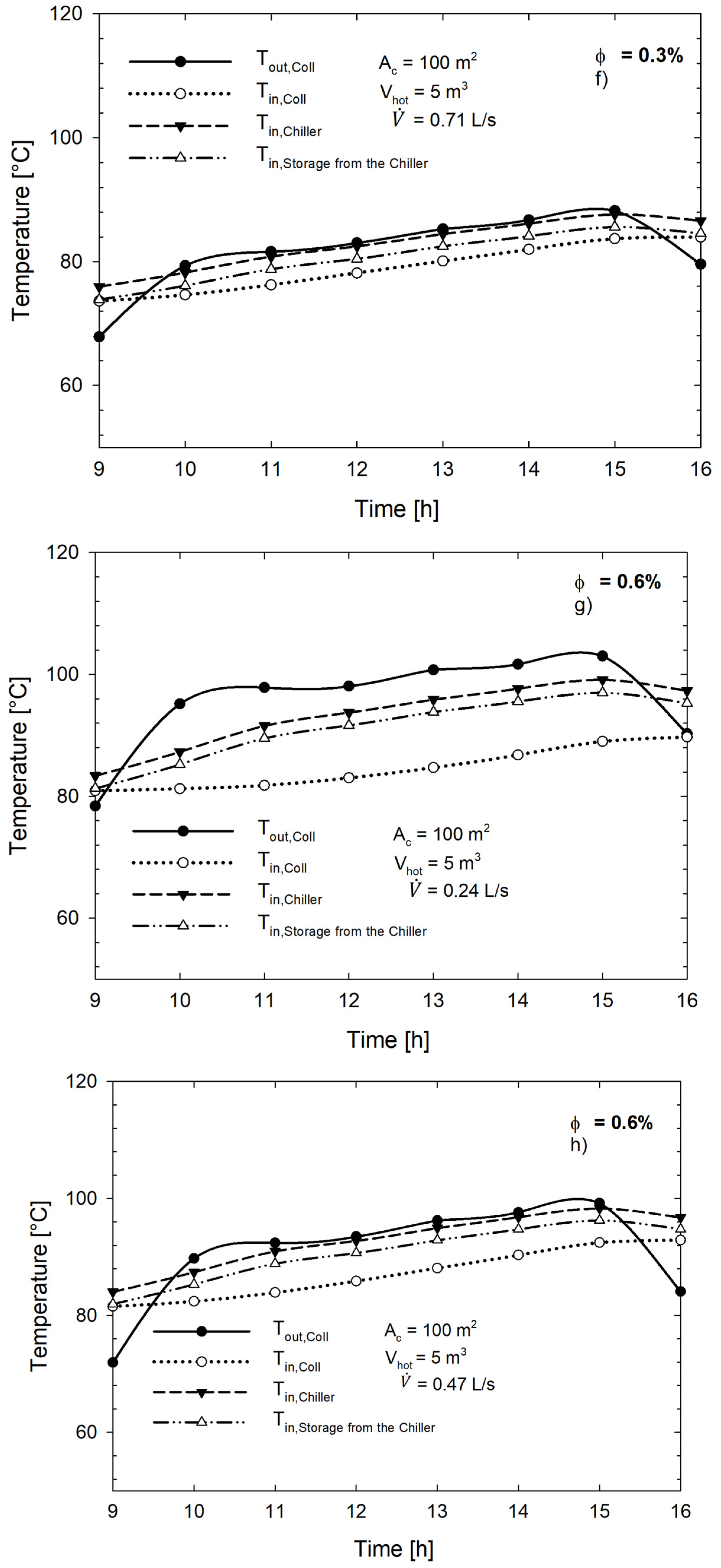
5. Results and Discussion
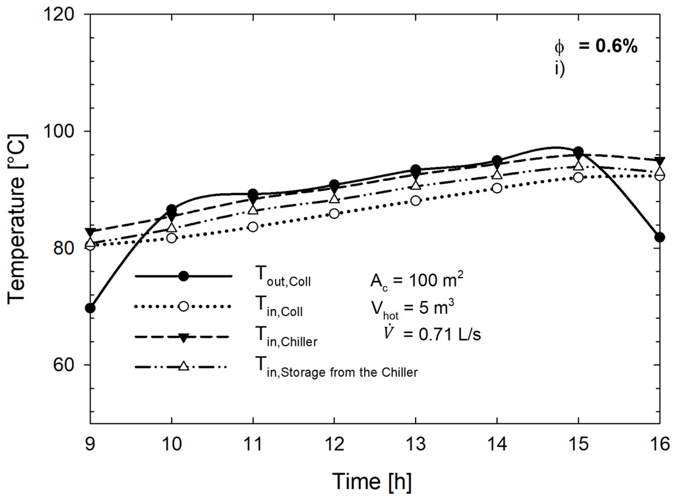
5.1. Temperatures
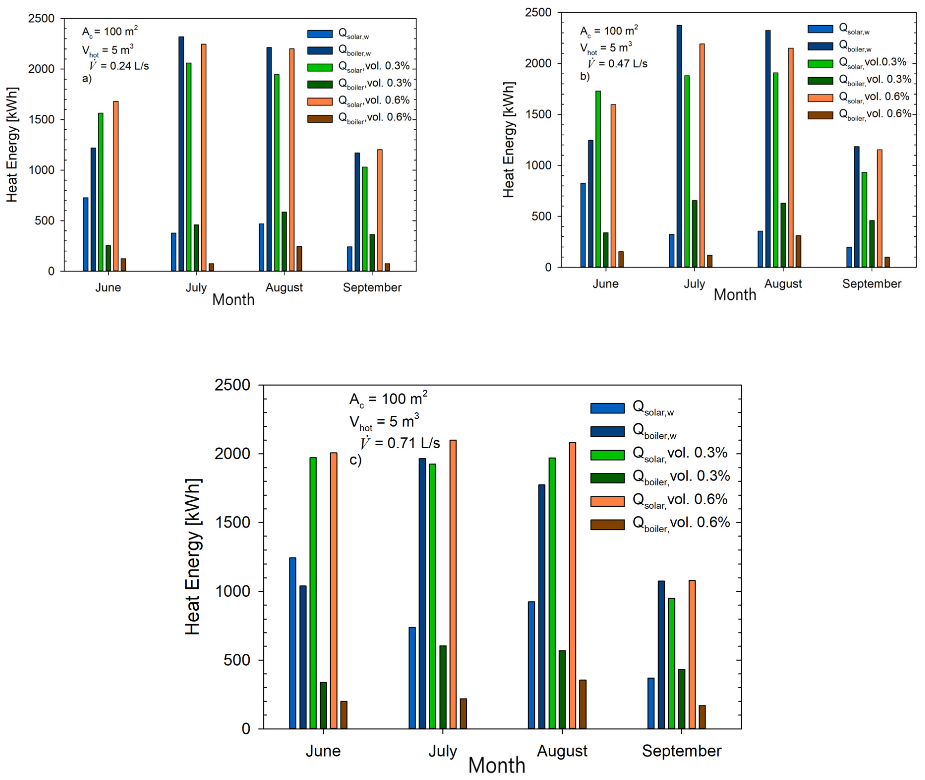
5.2. Heat Energy
5.3. Performance Results
6. Conclusions
- Enhanced Thermal Performance: The use of nanofluids led to significantly higher outlet temperatures from the solar collectors compared to pure water, due to improved thermal conductivity and heat transfer characteristics.
- Increased Solar Fraction: A solar fraction (SF) close to or equal to 1 was achieved in several configurations using nanofluids, especially at low volumetric flow rates, demonstrating a substantial reduction in reliance on auxiliary energy sources.
- Higher Primary Energy Savings: Configurations with nanofluids, particularly at 0.6% concentration, yielded seasonal primary energy savings exceeding 80%, highlighting the effectiveness of nanofluids in improving overall system efficiency.
- Acceptable Pumping Penalty: Although nanofluids increase the dynamic viscosity, the associated increase in pumping energy was modest (below 5%) and largely offset by thermal efficiency gains.
- Practical Applicability: The use of nanofluids in the solar loop only, combined with a realistic system layout and operating conditions, confirms their feasibility for real-world solar cooling installations.
- Future developments will include full-year simulations and the integration of techno-economic and life-cycle analyses to support broader deployment of nanofluid-enhanced solar thermal systems.
Author Contributions
Funding
Data Availability Statement
Conflicts of Interest
Nomenclature
| Ac | Solar collector area (m2) |
| B | Boiler (-) |
| C | Controller (-) |
| CH | Chiller (-) |
| COP | Coefficient of performance (-) |
| CST | Cold storage tank (-) |
| CT | Cooling tower (-) |
| cp | Specific heat (J kg−1 K−1) |
| DW | Distilled water (-) |
| ETCs | Evacuated tube solar collectors (-) |
| FC | Fan coil (-) |
| FPC | Flat plate solar collector (-) |
| HST | Hot storage tank (-) |
| k | Thermal conductivity (Wm−1 K−1) |
| f | Fractional primary energy saving for a solar cooling system (-) |
| G | Incident global solar radiation on the collector (W m−2) |
| P | Pump (-) |
| Qboiler | Heat energy of the auxiliary boiler (kWh) |
| Qsolar | Heat energy gain from solar collectors (kWh) |
| Qcooling,ref | Energy cold provided by a conventional system (kWh) |
| SCS | Solar cooling system (-) |
| SF | Solar fraction (-) |
| Tcoll,o | Outlet temperature of solar collector (°C) |
| Tcoll,i | Inlet temperature of solar collector (°C) |
| Tst,i | Inlet temperature of hot storage tank (°C) |
| Tst,o | Outlet temperature of hot storage tank (°C) |
| Volumetric flow rate (l s−1) | |
| Vol | Volumetric concentration (%) |
| Greek symbols | |
| η | Thermal efficiency of solar collector (-) |
| εheat | Efficiency of supplementary boiler (-) |
| εcooling | Efficiency of thermal power plant (-) |
| ϕ | Solid volume fraction (%) |
| ρ | Density (kg m−3) |
| µ | Dynamic viscosity (kg m−1s−1) |
| ΔT | Temperature difference between fluid and ambient temperature (°C) |
| Subscripts | |
| bf | Base fluid (water) |
| p | Nanoparticle |
| w | Water |
| nf | Nanofluid |
References
- Xuan, Y.; Li, Q. Heat transfer enhancement of nanofluids. Int. J. Heat Fluid Flow 2000, 21, 58–64. [Google Scholar] [CrossRef]
- Choi, S.U.; Eastman, J.A. Enhancing thermal conductivity of fluids with nanoparticles. In ASME International Mechanical Engineering Congress & Exposition; Argonne National Lab: Argonne, IL, USA, 1995. [Google Scholar]
- Almanassra, I.W.; Manasrah, A.D.; Al-Mubaiyedh, U.A.; Al-Ansari, T.; Malaibari, Z.O.; Atieh, M.A. An experimental study on stability and thermal conductivity of water/CNTs nanofluids using different surfactants: A comparison study. J. Mol. Liq. 2020, 304, 111025. [Google Scholar] [CrossRef]
- Karakaş, A.; Harikrishnan, S.; Öztop, H.F. Preparation of EG/water mixture-based nanofluids using metal-oxide nanocomposite and measurement of their thermophysical properties. Therm. Sci. Eng. Prog. 2022, 36, 101538. [Google Scholar] [CrossRef]
- Ju, X.; Liu, H.; Pei, M.; Li, W.; Lin, J.; Liu, D.; Ju, X.; Xu, C. Multi-parameter study and genetic algorithm integrated optimization for a nanofluid-based photovoltaic/thermal system. Energy 2023, 267, 126528. [Google Scholar] [CrossRef]
- Lin, H.; Jian, Q.; Bai, X.; Li, D.; Huang, Z.; Huang, W.; Feng, S.; Cheng, Z. Recent advances in thermal conductivity and thermal applications of graphene and its derivatives nanofluids. Appl. Therm. Eng. 2023, 218, 119176. [Google Scholar] [CrossRef]
- Alktranee, M.; Shehab, M.A.; Németh, Z.; Bencs, P.; Hernadi, K. Effect of zirconium oxide nanofluid on the behaviour of photovoltaic–thermal system: An experimental study. Energy Rep. 2023, 9, 1265–1277. [Google Scholar] [CrossRef]
- Das, L.; Aslfattahi, N.; Habib, K.; Saidur, R.; Irshad, K.; Yahya, S.M.; Kadirgama, K. Improved thermophysical characteristics of a new class of ionic liquid + diethylene glycol/Al2O3 + CuO based ionanofluid as a coolant media for hybrid PV/T system. Therm. Sci. Eng. Prog. 2022, 36, 101518. [Google Scholar] [CrossRef]
- Sarchami, A.; Tousi, M.; Kiani, M.; Arshadi, A.; Najafi, M.; Darab, M.; Houshfar, E. A novel nanofluid cooling system for modular lithium-ion battery thermal management based on wavy/stair channels. Int. J. Therm. Sci. 2022, 182, 107823. [Google Scholar] [CrossRef]
- Chinchole, A.S.; Dasgupta, A.; Kulkarni, P.P.; Chandraker, D.K.; Nayak, A.K. Exploring the Use of Alumina Nanofluid as Emergency Coolant for Nuclear Fuel Bundle. J. Therm. Sci. Eng. Appl. 2019, 11, 021007. [Google Scholar] [CrossRef]
- El Kholy, A.; Alyan, A.; Fakhry, K.; Abu-Elyazeed, O. Thermal hydraulic analysis of supercritical water reactor cooled by TiO2 nanofluid. J. Nucl. Sci. Technol. 2019, 56, 291–299. [Google Scholar] [CrossRef]
- Mostafizur, R.; Rasul, M.; Nabi, M.; Saianand, G. Properties of Al2O3-MWCNT/radiator coolant hybrid nanofluid for solar energy applications. Energy Rep. 2022, 8, 582–591. [Google Scholar] [CrossRef]
- Elshazly, E.; Abdel-Rehim, A.A.; El-Mahallawi, I. Thermal performance enhancement of evacuated tube solar collector using MWCNT, Al2O3, and hybrid MWCNT/Al2O3nanofluids. Int. J. Thermofluids 2023, 17, 100260. [Google Scholar] [CrossRef]
- Azeez, K.; Abu Talib, A.R.; Ibraheem Ahmed, R. Heat transfer enhancement for corrugated facing step channels using aluminium nitride nanofluid-numerical investigation. J. Therm. Eng. 2022, 8, 734–747. [Google Scholar] [CrossRef]
- Uniyal, A.; Prajapati, Y.K.; Ranakoti, L.; Bhandari, P.; Singh, T.; Gangil, B.; Sharma, S.; Upadhyay, V.V.; Eldin, S.M. Recent Advancements in Evacuated Tube Solar Water Heaters: A Critical Review of the Integration of Phase Change Materials and Nanofluids with ETCs. Energies 2022, 15, 8999. [Google Scholar] [CrossRef]
- Greco, A.; Gundabattini, E.; Gnanaraj, D.S.; Masselli, C. A comparative study on the performances of flat plate and evacuated tube collectors deployable in domestic solar water heating systems in different climate areas. Climate 2020, 8, 78. [Google Scholar] [CrossRef]
- Cirillo, L.; Della Corte, A.; Nardini, S. Feasibility study of solar cooling thermally driven system configurations for an office building in mediterranean area. Int. J. Heat Technol. 2016, 34, S472–S480. [Google Scholar] [CrossRef]
- Cascetta, F.; Di Lorenzo, R.; Nardini, S.; Cirillo, L. A Trnsys Simulation of a Solar-Driven Air Refrigerating System for a Low-Temperature Room of an Agro-Industry site in the Southern part of Italy. Energy Procedia 2017, 126, 329–336. [Google Scholar] [CrossRef]
- Hawwash, A.; Rahman, A.K.A.; Nada, S.; Ookawara, S. Numerical Investigation and Experimental Verification of Performance Enhancement of Flat Plate Solar Collector Using Nanofluids. Appl. Therm. Eng. 2018, 130, 363–374. [Google Scholar] [CrossRef]
- Eyyamoglu, B.; Bahlouli, K. Performance and economic analysis of a nanofluid-based solar-driven trigeneration system for a residential building in Cyprus. Appl. Therm. Eng. 2025, 277, 127001. [Google Scholar] [CrossRef]
- Shaalan, Z.A.; Hussein, A.M.; Abdullah, M.Z.; Alsayah, A.M.; Alshukri, M.J.; Khaled, M. Enhanced photovoltaic cooling using ZnO/TiO2 hybrid nanofluids: Numerical and experimental analysis. Int. J. Thermofluids 2025, 27, 101222. [Google Scholar] [CrossRef]
- Aissa, A.; Qasem, N.A.; Mourad, A.; Laidoudi, H.; Younis, O.; Guedri, K.; Alazzam, A. A review of the enhancement of solar thermal collectors using nanofluids and turbulators. Appl. Therm. Eng. 2023, 220, 119663. [Google Scholar] [CrossRef]
- Muhammad, M.J.; Muhammad, I.A.; Sidik, N.A.C.; Yazid, M.N.A.W.M. Thermal performance enhancement of flat-plate and evacuated tube solar collectors using nanofluid: A review. Int. Commun. Heat Mass Transf. 2016, 76, 6–15. [Google Scholar] [CrossRef]
- Cascetta, F.; Cirillo, L.; Nardini, S.; Vigna, S. Transient Simulation of a Solar Cooling System for an Agro-Industrial Application. Energy Procedia 2018, 148, 328–335. [Google Scholar] [CrossRef]
- Buonomo, B.; Cascetta, F.; Cirillo, L.; Nardini, S. Application of nanofluids in solar cooling system: Dynamic simulation by means of TRNSYS software. Model. Meas. Control B 2018, 87, 143–150. [Google Scholar] [CrossRef]
- Xuan, Y.; Roetzel, W. Conceptions for heat transfer correlation of nanofluids. Int. J. Heat Mass Transf. 2000, 43, 3701–3707. [Google Scholar] [CrossRef]
- Ghaderian, J.; Sidik, N.A.C. An experimental investigation on the effect of Al2O3/distilled water nanofluid on the energy efficiency of evacuated tube solar collector. Int. J. Heat Mass Transf. 2017, 108, 972–987. [Google Scholar] [CrossRef]
- Kasaeian, A.; Daneshazarian, R.; Pourfayaz, F. Comparative study of different nanofluids applied in a trough collector with glass-glass absorber tube. J. Mol. Liq. 2017, 234, 315–323. [Google Scholar] [CrossRef]
- Sarkar, J. A critical review on convective heat transfer correlations of nanofluids. Renew. Sustain. Energy Rev. 2011, 15, 3271–3277. [Google Scholar] [CrossRef]
- Khan, S.M.A.; Badar, A.W.; Siddiqui, M.S.; Siddique, M.Z.; Ul Haq, M.S.; Butt, F.S. Modeling and comparative assessment of solar thermal systems for space and water heating: Liquid water versus air-based systems. J. Renew. Sustain. Energy 2023, 15, 063702. [Google Scholar] [CrossRef]
- Available online: https://maya-airconditioning.com/assorbitori-ad-acqua/ (accessed on 5 June 2025).
- Shirazi, A.; Taylor, R.A.; Morrison, G.L.; White, S.D. A comprehensive, multi-objective optimization of solar-powered absorption chiller systems for air-conditioning applications. Energy Convers. Manag. 2017, 132, 281–306. [Google Scholar] [CrossRef]
- Fong, K.F.; Chow, T.T.; Lee, C.K.; Lin, Z.; Chan, L.S. Comparative study of different solar cooling systems for buildings in subtropical city. Sol. Energy 2010, 84, 227–244. [Google Scholar] [CrossRef]
- Sparber, W.; Thuer, A.; Besana, F.; Streicher, W.; Henning, H.M. Unified Monitoring Procedure and Performance Assessment for Solar Assisted Heating and Cooling Systems. In Proceedings of the 1st International Conference on Solar Heating, Cooling and Buildings, Lisbon, Portugal, 7–10 October 2008. [Google Scholar]
- White, F.M. Fluid Mechanics, 8th ed.; McGraw-Hill Education: New York, NY, USA, 2016. [Google Scholar]


| Material | ρ (kg/m3) | k (W/mK) | cp (J/kgK) | μ (Pa s) | Ref. |
|---|---|---|---|---|---|
| Al2O3 | 3970 | 36 | 773 | [26] | |
| Water | 997 | 0.60 | 4178 | 8.94 ∙ 10−4 | - |
| Water–Al2O3 (vol. 0.3%) | 1010 | 0.62 | 4121 | 9.01 ∙ 10−4 | [27] |
| Water–Al2O3 (vol. 0.6%) | 1025 | 0.64 | 4066 | 9.01 ∙ 10−4 | [27] |
| Working Fluid | [L s−1] | Nanoparticles | Vol. % | Equation |
|---|---|---|---|---|
| (Al2O3/DW) | 0.24 | Al2O3 | 0.3 | |
| (Al2O3/DW) | 0.47 | Al2O3 | 0.3 | |
| (Al2O3/DW) | 0.71 | Al2O3 | 0.3 | |
| (Al2O3/DW) | 0.24 | Al2O3 | 0.6 | |
| (Al2O3/DW) | 0.47 | Al2O3 | 0.6 | |
| (Al2O3/DW) | 0.71 | Al2O3 | 0.6 | |
| Water | 0.24 | - | - | |
| Water | 0.47 | - | - | |
| Water | 0.71 | - | - |
| Specification | Unit | Dimension |
|---|---|---|
| Gross area | m2 | 2.57 |
| Aperture area | m2 | 2.22 |
| Absorber area | m2 | 2.36 |
| Length | m | 1.80 |
| Width/width incl. connection | mm | 1560/1612 |
| Max operating pressure | bar | 10 |
| Absorber | - | Aluminum |
| Absorption (α)/emission (ε) | - | 0.96/0.06 |
| Collector housing | - | Aluminum |
| Collector glazing | - | Evacuated tubes |
| Number of tubes | - | 18 |
| Outer glass tube diameter | mm | 6 |
| Inner glass tube diameter | mm | 5 |
| Sealing material | - | Silicone |
| Frame material | - | Stainless steel |
| Component | Thickness [cm] | Mass [kg/m2] | Thermal Trasmittance [W/(m2K)] |
|---|---|---|---|
| External wall | 33 | 370 | 1.26 |
| Ceiling | 35 | 506 | 1.25 |
| Floor | 35 | 506 | 1.25 |
| Window (double glass)—Argon gas | 1.2 | - | 2.072 |
| Aluminum frame | - | - | 2.405 |
| Component | Description |
|---|---|
| Hot water absorption chiller (Type 107) | |
| Peak cooling load | 17.5 kW |
| COP | 0.71 |
| Chilled water setpoint temperature | 0.667 |
| Minimum operative temperature | 90 °C |
| Specific heat of hot water, cooling water and chilled water | 4.18 kJ kg−1 K−1 |
| Evacuated tube solar collectors (ETCs—Type 71) | |
| Collector area | 100 m2 |
| Number in series | 1 |
| Efficiency mode (Inlet temperature) | 1 |
| Collector efficiency | Table 2 |
| Solar collector slope | 40° |
| Pump (Type 740) | |
| Hot water flowrate between hot storage tank and ETCs | 0.24/0.47/0.71 L s−1 |
| Specific heat of fluid (water) | 4.18 kJ kg−1 K−1 |
| Specific heat of fluid (0.3% vol.) | 3.81 kJ kg−1 K−1 |
| Specific heat of fluid (0.6% vol.) | 3.50 kJ kg−1 K−1 |
| Fluid density (water) | 1000 kg m−3 |
| Fluid density (0.3% vol.) | 1087.45 kg m−3 |
| Fluid density (0.6% vol.) | 1176.60 kg m−3 |
| Pump_2 (Type 740) | |
| Hot water flowrate between hot storage tank and chiller | 0.5 L s−1 |
| Specific heat of fluid (water) | 4.18 kJ kg−1 K−1 |
| Fluid density (water) | 1000 kg m−3 |
| Hot storage tank (Type 4a) | |
| Tank type | Stratified |
| Tank loss coefficient | 0.694 W m−2 K |
| Volume | 5 m3 |
| Fluid density (water) | 1000 kg m−3 |
| No. nodes | 6 |
| Supplementary boiler (Type 122) | |
| Setpoint temperature | 90 °C |
| Maximum heating rate | 24 kW |
| Deadband for heating | 5°C (ΔT) |
| Cold storage tank (Type 4a) | |
| Tank type | Stratified |
| Tank loss coefficient | 0.694 W m−2 K |
| Volume | 2 m3 |
| Fluid density (water) | 1000 kg m−3 |
| No. nodes | 1 |
| Cooling Tower (Type 510a) | |
| Rated Fan Power | 1.36 kW |
| Fluid specific heat | 4.19 kJ/(kg K) |
| Time step of the simulation | 1 h |
| Duration of the simulation | 1 June–30 September |
| Parameter | Nominal Value | Variation | ∆SF (%) | Relative Sensibility (S) |
|---|---|---|---|---|
| Solar radiation | 800 W/m2 | 720–880 W/m2 | 0.75 | |
| Nanofluid viscosity (range 30–90 °C) | 0.9 mPa∙s | 0.81–0.99 mPa∙s | 0.52 | |
| Collector efficiency (seasonal) | 0.70 | 0.63–0.77 | 0.45 | |
| Heat loss Storage Tank | 1.0 W/(m2 K) | 0.9–1.1 W/(m2 K) | 0.22 |
| Results | = 0.24 L s−1 | = 0.47 L s−1 | = 0.47 L s−1 | |||
|---|---|---|---|---|---|---|
| 0.3% vol. | 0.6% vol. | 0.3% vol. | 0.6% vol. | 0.3% vol. | 0.6% vol. | |
| Temperature | ||||||
| Collector outlet temperatureSu | 19.88% | 33.06% | 11.88% | 24.37% | 10.34% | 18.89% |
| Collector inlet temperature | 5.70% | 18.56% | 8.23% | 22.43% | 7.75% | 18.33% |
| Storage outlet temperature | 10.07% | 23.07% | 7.98% | 21.42% | 7.98% | 18.13% |
| Energy | ||||||
| Solar gain from collectors | 300.69% | 348.18% | 349.28% | 414.13% | 478.80% | 503.67% |
| Supplementary boiler | −75.44% | −92.27% | −69.83% | −90.19% | −66.02% | −83.46% |
| Pumping consumption | 9.74% | 9.20% | 16.89% | 15.29% | 11.90% | 10.35% |
Disclaimer/Publisher’s Note: The statements, opinions and data contained in all publications are solely those of the individual author(s) and contributor(s) and not of MDPI and/or the editor(s). MDPI and/or the editor(s) disclaim responsibility for any injury to people or property resulting from any ideas, methods, instructions or products referred to in the content. |
© 2025 by the authors. Licensee MDPI, Basel, Switzerland. This article is an open access article distributed under the terms and conditions of the Creative Commons Attribution (CC BY) license (https://creativecommons.org/licenses/by/4.0/).
Share and Cite
Cirillo, L.; Gargiulo, S.; Greco, A.; Masselli, C.; Nardini, S.; Orabona, V.; Verneau, L. A Dynamic Investigation of a Solar Absorption Plant with Nanofluids for Air-Conditioning of an Office Building in a Mild Climate Zone. Energies 2025, 18, 3480. https://doi.org/10.3390/en18133480
Cirillo L, Gargiulo S, Greco A, Masselli C, Nardini S, Orabona V, Verneau L. A Dynamic Investigation of a Solar Absorption Plant with Nanofluids for Air-Conditioning of an Office Building in a Mild Climate Zone. Energies. 2025; 18(13):3480. https://doi.org/10.3390/en18133480
Chicago/Turabian StyleCirillo, Luca, Sabrina Gargiulo, Adriana Greco, Claudia Masselli, Sergio Nardini, Vincenzo Orabona, and Lucrezia Verneau. 2025. "A Dynamic Investigation of a Solar Absorption Plant with Nanofluids for Air-Conditioning of an Office Building in a Mild Climate Zone" Energies 18, no. 13: 3480. https://doi.org/10.3390/en18133480
APA StyleCirillo, L., Gargiulo, S., Greco, A., Masselli, C., Nardini, S., Orabona, V., & Verneau, L. (2025). A Dynamic Investigation of a Solar Absorption Plant with Nanofluids for Air-Conditioning of an Office Building in a Mild Climate Zone. Energies, 18(13), 3480. https://doi.org/10.3390/en18133480