Article

Long-Term Forecast of Peak Power Demand for Poland—Construction and Use of Simplified Forecasting Models

by
Tomasz Popławski
Department of Electrical Engineering, Czestochowa University of Technology, 42-200 Czestochowa, Poland
Energies 2025, 18(13), 3472; https://doi.org/10.3390/en18133472
Submission received: 3 June 2025 / Revised: 20 June 2025 / Accepted: 30 June 2025 / Published: 1 July 2025
(This article belongs to the Special Issue Improvements of the Electricity Power System: 3rd Edition)

Abstract

This article presents a simplified method for forecasting Poland’s long-term peak electricity demand using a modified Prigogine logistic equation. While complex models like the WEM or PRIMES offer high precision, their complexity and data requirements can be limiting. The proposed model offers a quicker and more accessible alternative, using the average annual load factor ( A L F ) as a key indicator. Based on historical data (1985–2024), the model was validated and optimized (MAPE < 2%), then applied to forecast the demand through 2040 under three scenarios: coal-based energy, nuclear energy and energy from RESs (renewables). Depending on the scenario, the peak demand is expected to rise from 28.7 GW in 2024 to 34–40 GW in 2040. The model’s strength lies in its ability to capture dynamic system behavior, including chaos and bifurcations, making it suitable for rapid assessments and strategic planning. Despite its limitations—such as a lower level of detail and an inability to integrate sectoral policies—the Prigogine-based approach offers a transparent, cost-effective forecasting tool, especially when complemented by the use of advanced simulation models.

1. Introduction

For years, the Polish power industry has been based mainly on fossil fuels, primarily hard coal and lignite. According to data from 2024, about 63% of the electricity in Poland came from coal and about 20% from renewable energy sources (mainly photovoltaics and wind energy). The power system is centralized and based on large conventional power plants, with a relatively low level of flexibility and a limited number of energy storage facilities.
The Business-as-Usual (BaU) scenario assumes a continuation of the current trends without radical reforms and without a significant acceleration of the energy transformation. According to such a model, Poland will continue to invest in the modernization of existing coal-fired units and in the slow development of RESs but not in systemic solutions supporting the integration of these sources with the network (e.g., solutions tackling a lack of energy storage facilities, delays in the development of transmission networks and unstable auction policies).
In the near term, by 2030, the share of coal may fall to around 50–55%, mainly due to the retirement of the oldest and least efficient units. Renewable energy sources may reach a share of 25–30%, mainly due to the further development of photovoltaics and the unblocking of onshore wind power. Gas-fired power plants may become more important as stabilizing sources, but this is associated with a risk of dependence on gas imports.
Maintaining a high share of coal will be associated with rising CO2 emission costs. ETS allowance prices will probably exceed EUR 100 per tonne by 2030. This means increasing pressure on energy prices and deepening energy poverty. In the BaU scenario, supply gaps in the electricity system are possible (especially in winter), especially after 2027, when the capacity market mechanism for most coal-fired power plants will expire.
The lack of sufficient new generation and storage capacities may lead to increased energy imports. Without large investments in transmission and distribution networks, the development of renewable energy will be limited. Unstable regulation will remain a problem. Another problem will be the volatility of the law and the lack of a long-term strategy, which will translate into unstable private investments. Unfortunately, nuclear energy will not solve these problems either. The first nuclear power plant unit is not scheduled to start operating until after 2033. In the BaU scenario, preparations for construction may be delayed for procedural, financial or political reasons, which will additionally increase the pressure to maintain old coal units.
A Business-as-Usual scenario for Poland until 2030 will mean maintaining a high share of coal, increasing energy costs, the system not adapting to new technologies and the risk of not meeting climate obligations towards the EU. If Poland wants to avoid an energy crisis and keep up with the European energy transformation, a clear change of course is needed towards a sustainable energy mix, investment in infrastructure and the development of energy storage facilities.
In order to make correct estimates, the problem of using appropriate analytical tools for these purposes arises. The following part of this article describes the most commonly used ones and proposes a simplified model supporting these analyses.

1.1. Complex Forecasting Models in Energy and Climate Analysis

Power system modeling is a time-consuming task that requires interdisciplinary knowledge (including knowledge of mathematics, physics, computer science, energy, economics, energy policies, etc.) and a very good understanding of the modeled sector [1]. It is a complex operation that requires the use of an appropriate methodology to avoid errors that may occur at virtually every stage of model construction. In order to correctly make the desired prediction, the phenomenon must first be correctly modeled. Using a model to solve real problems allows for correct inferences about the original behavior of the thing being modeled, which is usually not available when conducting experiments.
The effects of decision-making are usually difficult to predict, primarily due to the complexity of relationships in this sector and the connections with other sectors. Contemporary challenges such as climate change, the growing demand for energy, the development of low-emission technologies and the global energy transformation require the use of increasingly advanced analytical tools in the case of the long-term planning of the development and operation of power systems.
Complex forecasting models allow us to predict the development of energy systems in the long term, taking into account technological, economic, political and environmental factors. The most well-known and frequently used models include the World Energy Model (WEM), PRIMES, POLES and Green-X. The WEM [2] was developed by the International Energy Agency (IEA). It is a simulation tool used to forecast the energy demand and supply until 2050 and beyond. It takes into account economic factors (GDP, prices, population) and technological and regulatory factors, including climate policies. The WEM is used, among other models, in preparing the “World Energy Outlook” report and analyzing energy transformation scenarios [3]. The PRIMES model [4], developed by E3MLab at the University of Athens, is an integrated market equilibrium model of the energy systems of the European Union. It allows for the forecasting of the development of the energy sector, emissions and decarbonization costs. It is used by the European Commission, among other models, in the analysis of climate scenarios up to 2030 and 2050 and in the assessment of the impacts of initiatives such as “Fit for 55” [5]. The POLES model [6] (Prospective Outlook on Long-Term Energy Systems), developed by the CNRS, Université Grenoble Alpes and Enerdata, is a partial equilibrium model analyzing global energy and climate scenarios up to 2100. It includes a high level of sectoral detail and the ability to simulate decarbonization trajectories and the deployment of low-emission technologies [7]. The Green-X model [8], developed by TU Wien, is a tool for analyzing policies supporting the use of renewable energy sources (RESs) in Europe. It is based on an econometric cost-optimization approach. It allows for long-term horizon forecasting [9] together with an assessment of the effectiveness of support mechanisms (e.g., auctions, feed-in tariffs), the potential of RESs and cross-border cooperation in the EU.

1.2. The Role of Simplified Forecasting Models

Complex forecasting models are the foundation of long-term energy planning. They support decision-makers, EU institutions and international organizations in assessing the effects of climate policies, allocating investment funds and analyzing systemic risks. Their use allows for better preparation for structural changes in the energy sector and supports the implementation of the goals of the Paris Agreement, among others. Unfortunately, the disadvantages of these models are their complexity and the requirement to collect extensive databases on economic, technical and social phenomena, which in some situations prevent their use. An alternative to them are simplified forecasting models, which allow for a quick, approximate determination of energy trends and needs. These models, despite their simplicity, are an important tool in long-term energy planning. Their use allows for a quick assessment of development trends and supports strategic decision-making. In combination with more accurate models, they can be used to create an effective decision support system in the power sector. Simplified long-term forecasting models are most often based on the following:
  • Econometric methods using a regression between the demand and variables such as the GDP, population or energy prices [1,9,10,11,12];
  • Historical trend methods, in which future values are predicted based on previous observations (e.g., trend extrapolation methods) [13,14,15,16];
  • Indicator methods, where the energy consumption is estimated on the basis of individual indicators (e.g., the consumption per household, per unit of GDP, etc.) or by determining indicators that are leading, cyclical, synthetic, etc. [17,18,19,20,21];
  • Hybrid models combining various forecasting techniques including machine learning (ML) and artificial intelligence (AI) [22,23,24,25,26].
The advantages of these methods are their low cost, the speed of the calculations and the transparency of the results, although these come at the cost of lower precision and a lack of consideration of dynamic dependencies. Table 1 below compares the most important features of simple and advanced prediction models used for long-term forecasts.
In their current research practices, the author has successfully used models described in detail in [1] for long-term prediction purposes. The following part of this article attempts to predict the long-term peak power demand for Poland with a horizon of 2040. This prediction employs an innovative simplified prediction model using a modified Prigogin equation based on a nonlinear logistic equation from determinate chaos theory describing the development of the studied population (excluding deaths). Theoretical solutions justifying the adoption of such a solution are presented, as well as the forecast results based on such a solution, their accuracy and the methodology of the procedure.

2. The Logistic Equation as a Universal Tool in the Analysis of Population Dynamics and Long-Term Forecasts

The proposal of the logistic equation by Pierre François Verhulst in 1838 [30] was a pioneering step in the mathematical modeling of population growth. Verhulst proposed it as a response to the unrealistic assumptions of the earlier Malthus model, which predicted exponential (unlimited and unsustainable) population growth.
d N d t = r N 1 N K
where N is the number of individuals (population) at time t, r is the growth factor and K is the carrying capacity of an environment (the maximum number of individuals that the environment can support).
The logic of the model described by Formula (1) is as follows:
  • Initial growth—when N K the population grows almost exponentially.
  • Growth slowdown—as the carrying capacity of the environment approaches N K , growth slows down.
  • Steady state—when N = K population growth stops and d N d t = 0 .
This equation has gained new meaning and complexity thanks to the work of Ilya Prigogin, among others, in the context of open and nonlinear systems. Currently, this model and its numerous extensions play a key role in modeling biological, social and environmental processes. Scientific articles published in recent years confirm its wide application in describing population growth, especially in conditions with limited resources, a reactive environment or an environment with a dynamic carrying capacity. Most often, its modifications focus on developing the classic logistic model by considering the following:
  • Time delays [31];
  • The development of animal populations with random fluctuations [32];
  • Mutualistic or competitive interactions [33];
  • The modeling of human populations and the socio-technological conditions [34,35,36];
  • Stochasticity and uncertainty [37];
  • The variable carrying capacity of the environment [38].
Prigogin’s logistic equation is often generalized in the spirit of his thermodynamic ideas, treating the population as a nonlinear system far from equilibrium which exchanges matter and energy with the environment. In [31,32,33] the authors described phenomena related to the development of animal populations and the surrounding environment. In [31] a model with a time delay and regulated harvesting was described. It was used to plan sustainable fisheries and forest management. Analyses showed that a failure to take into account delays can lead to incorrect forecasts and overexploitation. In [32] biological populations were analyzed, taking into account the random fluctuations of environmental parameters. A random logistic equation allows for a better reflection of the real variability of population numbers. In [33] the authors proposed a modified logistic equation for two mutually supportive populations (e.g., plants and pollinating insects). The classical model is insufficient; therefore they introduced nonlinear positive feedback.
In studies [34,35,36,37,38] the authors focused on modeling the human population in various socio-technological conditions, taking into account stochasticity and uncertainty and the variable carrying capacity of the environment. In article [36] the authors analyzed the fundamental principles of dynamics that lead to the derivation of a logistic equation (LE), widely used in population growth modeling. In particular, they showed that scalability (scale invariance) and the mean value constraint are both sufficient and necessary conditions for deriving an LE. The authors proved that by assuming the scalability of the system and the existence of the mean value constraint, a logistic equation can be derived as a natural description of the dynamics of such a system. They presented examples of the application of the generalized LE in various social contexts, such as modeling the distribution of city sizes, analyzing the spread of information or innovations in social networks and predicting the number of users of web browsers (e.g., Internet Explorer, Firefox, Chrome) in the context of the so-called “browser wars”.
In [39], the authors developed the classical Verhulst logistic equation by introducing a fertility or reproductive capacity factor, known as the Allee effect. They transformed the logistic equation into a product of two components: a depensation component responsible for the decrease in the growth rate at a low population size and a compensatory component responsible for the slowdown in growth near the carrying capacity of the environment. This approach allows for the more realistic modeling of evolutionary processes, taking into account both environmental and biological constraints. The logistic equation remains one of the most versatile tools for analyzing population dynamics. Its flexibility and the possibility of extensions [40] (Q-logistics, time functions, generalized parameters) make it extremely useful not only in ecology but also in sociology, economics, epidemiology, urban planning and other analyses concerning the evolution of systems, including power systems. Importantly, Prigogin’s approach brings additional value: it shows that populations and social systems can be treated as dynamic systems subject to the principles of non-equilibrium thermodynamics. This opens the way to new, interdisciplinary methods of analysis.
This paper proposes the use of a modified Prigogin [41] equation based on a nonlinear logistic equation. This equation has been analyzed and tested in many studies on long-term forecasting in power systems [1,42,43]. It describes the development of the studied population (excluding deaths):
X n + 1 = X n 1 + R 1 X n K , X n 0
where X n and X n + 1 are the population sizes at times n = t and n + 1 = t + τ , R is the growth rate coefficient, K is the development ceiling and τ is the interval representing the difference between a pair of values, X n and X n + 1 .
Based on the studies carried out in [1,42,43], it was found that the process described by Equation (2), depending on the value of the R coefficient and the ratio at the starting moment t = f 0 , can lead to six basic states of the behavior of X t + 1 :
  • SE—asymptotic monotonic convergence to K, the equilibrium of the system;
  • SB—striving for balance;
  • O—convergence to K with oscillations;
  • BI—bifurcation;
  • AB—a jump to K in the first few steps;
  • CH—chaos (including impossible events, such as X t + 1 < 0 ).
An example of the behavior of the process modeled by the Prigogin equation depending on the R coefficient and the K / X t 0 ratio is shown in Figure 1 and Figure 2.

2.1. Using the Prigogin Equation to Build a Long-Term Peak Power Demand Forecast for Poland

The increase in the demand for electrical power in Poland is the result of several factors. Firstly, the country’s economic development and the increasing number of energy recipients, both in the industrial and municipal sectors, contribute to the increased consumption of electricity. Secondly, the progressive electrification of various sectors of the economy, including transport and heating, increases the load on the power system. Additionally, climate change and the associated extreme weather phenomena, such as heat waves or frosts, lead to seasonal peaks in the energy demand. The basic indicator that combines the annual demand for electricity and the annual peak power demand in the power system is the average annual load factor ( A L F ). According to its definition [1,42], it is determined based on the following relationship:
A L F r = A r T r P r
where A r is the annual electricity demand in the national power system [MWh], P r is the annual peak power demand in the national power system [MW] and T r is the number of hours in a year, 8760 [h].
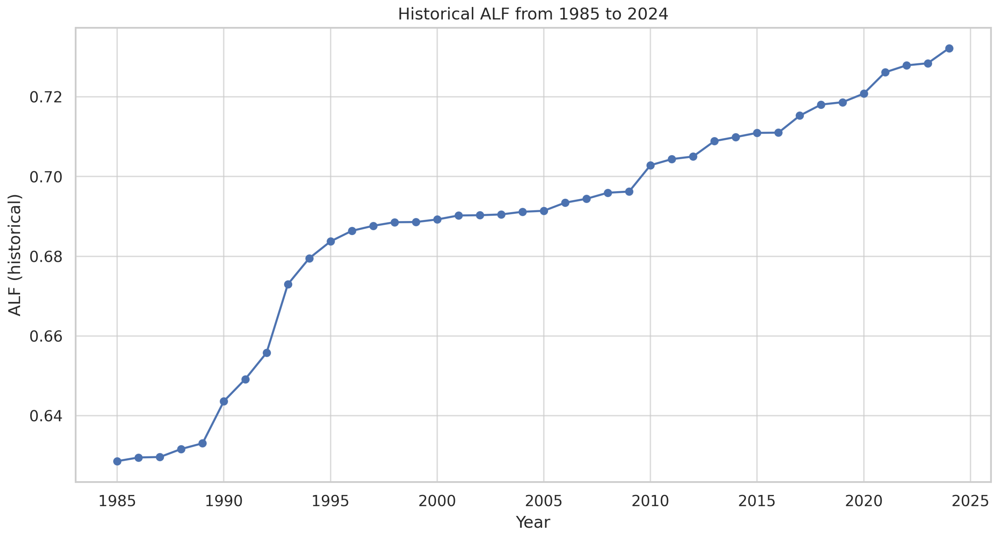
Based on the annual statistics for the Polish power system from 1985 to 2024, the average annual load factor, the A L F , was determined. As can be seen in Figure 3, over the forty-year research period, the A L F varied from 0.628 to 0.732.
As described in the previous chapters, the Prigogin equation described by the relation in (2) can be used to describe the development of various mass processes. These include the development and evolution of a power system. In the case of the average annual load factor of a power system ( A L F ), it has naturally existing limits. The value of this coefficient cannot be outside the range from 0 to 1. Based on the history of the process, it is possible to determine the level of development or saturation, K, to which the value of this parameter tends as long as there is no change in the value of this level. Therefore, the Prigogin equation can be adapted to determine the long-term forecast of the A L F :
A L F r , n + 1 = A L F r , n 1 + R 1 A L F r , n K , A L F r , n 0
where A L F r , n and A L F r , n + 1 are the A L F coefficient values at the time instants n = t and n + 1 = t + τ , R is the growth rate coefficient, K is the development ceiling and τ is the interval representing the difference between a pair of values, A L F r , n and A L F r , n + 1 .
The problem is to correctly determine the parameter K, called the level of development (saturation). As stated earlier, there is a natural limit that the ALF cannot exceed. This is the value K = 1 , to which the A L F will tend. However, adopting such a value would involve a very large approximation and very large prediction errors. In connection with the above, it is proposed to use the trend extrapolation method and determine, based on the history of the process, the logarithmic function to which the saturation value K tends with the smallest error when matching it to the history of the examined process. The form of the logarithmic function was selected using the linear regression method, obtaining the determination coefficient R 2 = 0.915 .
A L F n = 0.0326 ln ( n ) + 0.5988
For the determined logarithmic regression function, the model was validated for the years 2014 to 2024. The results of this validation are presented in Table 2.
For the 10-year validation process, a very low average fitting error, MAPE = 0.76%, was obtained. This indicates a good choice of the logarithmic function for fitting the model to the actual A L F data. The validation accuracy was considered satisfactory; therefore a highly probable interval was determined in which the ceiling of the level of development, K, of the tested average A L F would be found with a high level of accuracy.
For the tested number of observations, A L F = 40 , the standard deviation of the residuals was σ = 0.0089 , and the critical value of the Student’s t-test distribution with n 2 = 38 degrees of freedom was t 0.975 ( 38 ) 2.024 . The predicted value of the A L F interval was calculated using the following simplified formula:
± A L F n = A L F n ± t σ 1 + 1 n
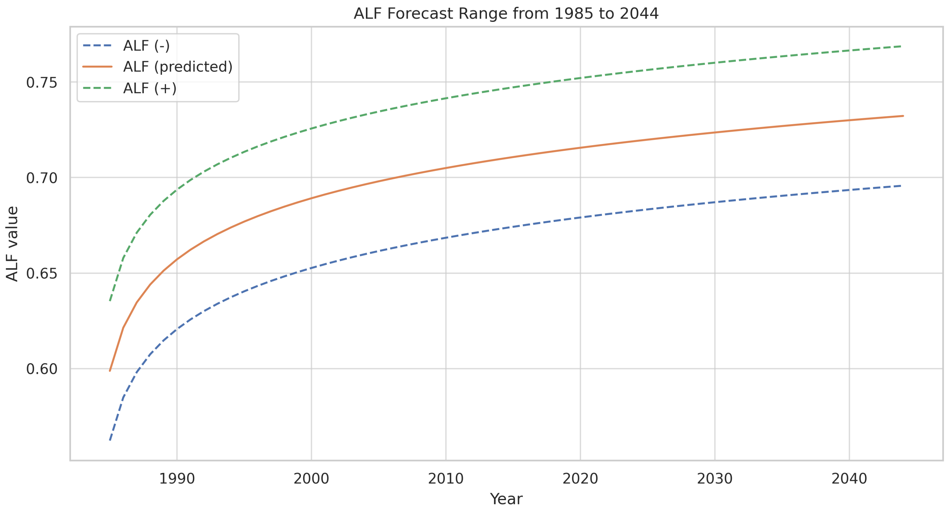
As can be seen in Figure 4, the forecast A L F variability range until 2044 was A L F ( ) = 0.6957 for the lower variability limit and A L F ( + ) = 0.7688 for the upper variability limit. Figure 4 also clearly shows that the course of the A L F variability in the last years forecast in this process approached the upper limit of its range. Therefore, it can be concluded that the forecast ceiling of the level of development, K, in the Prigogin equation in Formula (4) will tend to the value K = A L F ( + ) = 0.7688 .
The growth rate R was therefore determined. Using the modified Prigogin Equation (4), the R parameter was optimized using the nonlinear GRG (Generalized Reduced Gradient) method. This coefficient was determined iteratively based on historical data so that the estimated error in fitting the model to the actual historical data was as small as possible. Assuming that K = 0.7688 and τ = 15 , a value of K = 0.3938 was obtained for an MAPE = 0.78% fitting error.
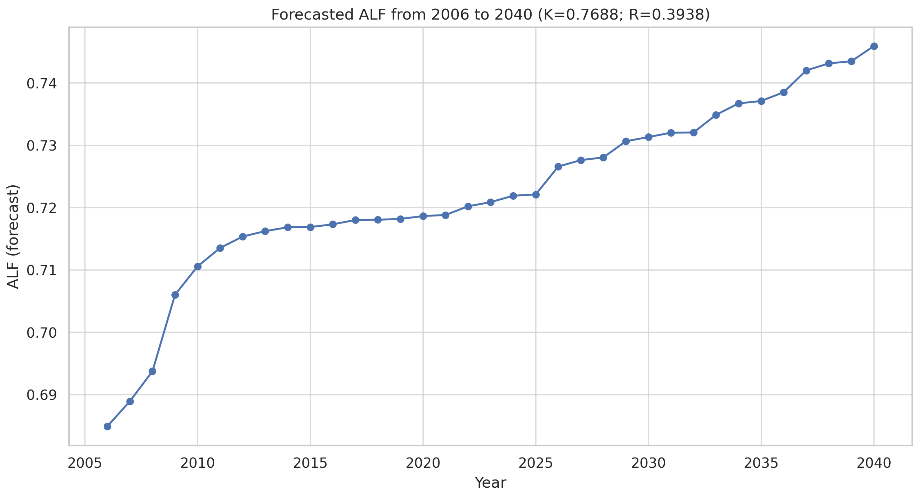
The forecast course of the average ALF until 2040 with the growth factor R = 0.3938 and the development ceiling K = 0.7688 is illustrated in Figure 5.

2.2. Long-Term Gross Electricity Demand Scenarios for Poland Until 2040

The forecasts of the electricity demand in Poland until 2040 presented in Table 3 vary depending on the adopted assumptions regarding the pace of energy transformation, technological development and energy policies. Official government documents [44] predict a significant increase in the demand, mainly due to the electrification of various sectors of the economy. Independent analyses [45,46] suggest that more ambitious goals for the development of renewable energy sources and greater energy efficiency may lead to different demand scenarios.
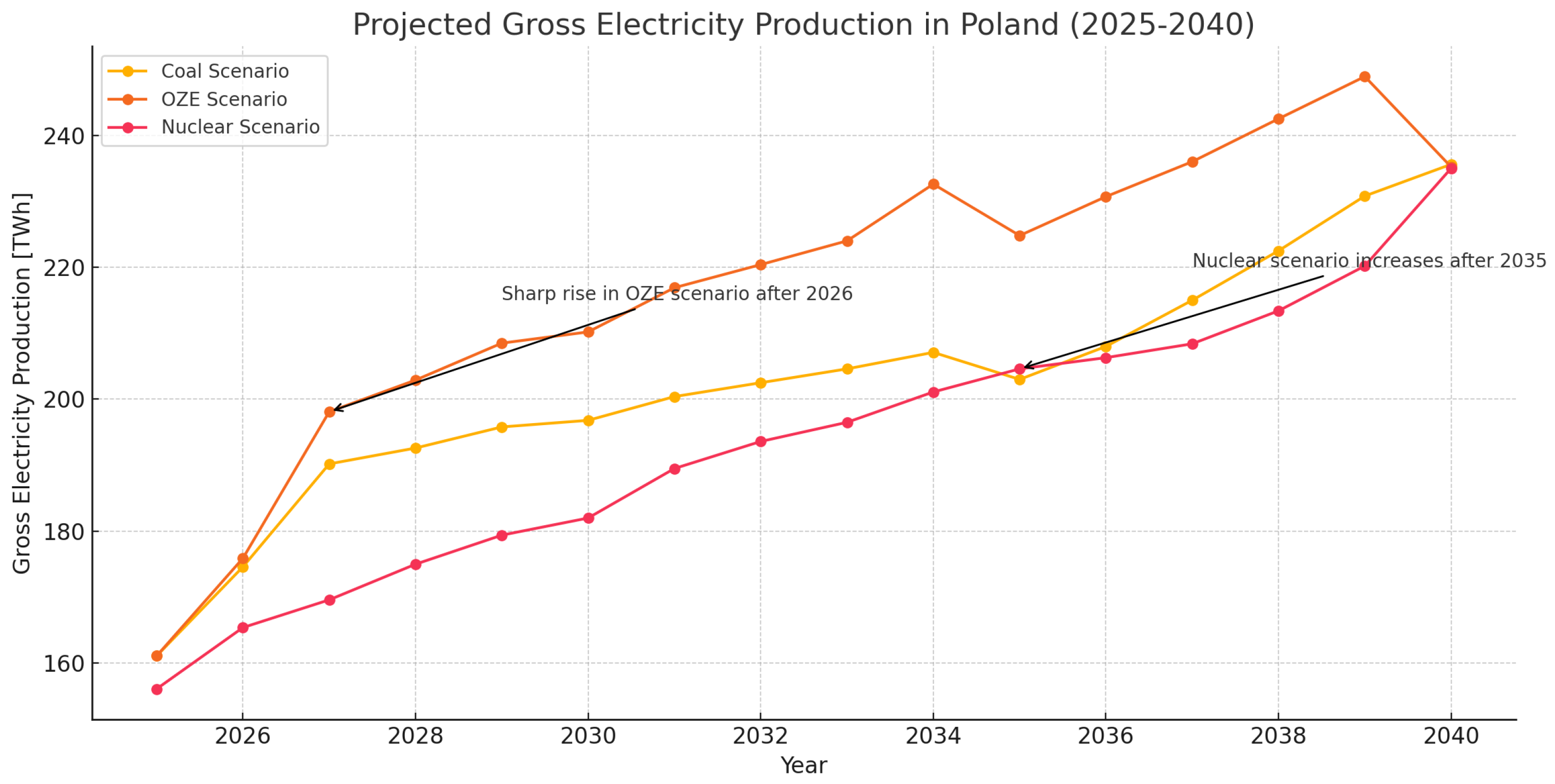
The scenarios analyzed above were very similar in terms of their final effect on the long-term forecast of the gross energy demand for Poland. Each of the institutions developing these scenarios emphasized different aspects in their studies. After detailed analyses, the scenarios developed in [46] were used further for the purposes of this article. Figure 6 illustrates the course of these forecasts. Based on these, the author’s forecasts of the peak power demand for Poland until 2040 were made and are discussed later in this article.

3. Author’s Forecast of Long-Term Peak Power Demand for Poland Until 2040

In order to verify the properties of the constructed prediction model based on the Prigogin Equation (4) and to determine its suitability for producing long-term forecasts, a validation forecast of the peak power demand for the years 2014 to 2024 was made. The equation used the growth coefficient R = 0.3938 and the development ceiling K = 0.7688 , determined based on the process history. The results are presented in Table 4.
As can be seen in Table 4, satisfactory forecast accuracies were obtained, and for the ten-year validation process the average forecast error was MAPE=1.85%. Based on the long-term prediction of the A L F and three scenarios regarding the gross electricity production for Poland, a forecast of the peak power demand in the national power system until 2040 was made using the relationship in (7).
P r , t = A r , t 1 T r 1 A L F r , t
where P r , t is the annual forecast of the peak power demand, A r , t is the annual forecast of the gross electricity demand according to three forecast scenarios—coal, nuclear and renewable energy— A L F r , t is the forecast of the average annual load factor, T r is the duration of a year (8760 h) and t = 1 . . . 15 is the forecast horizon.
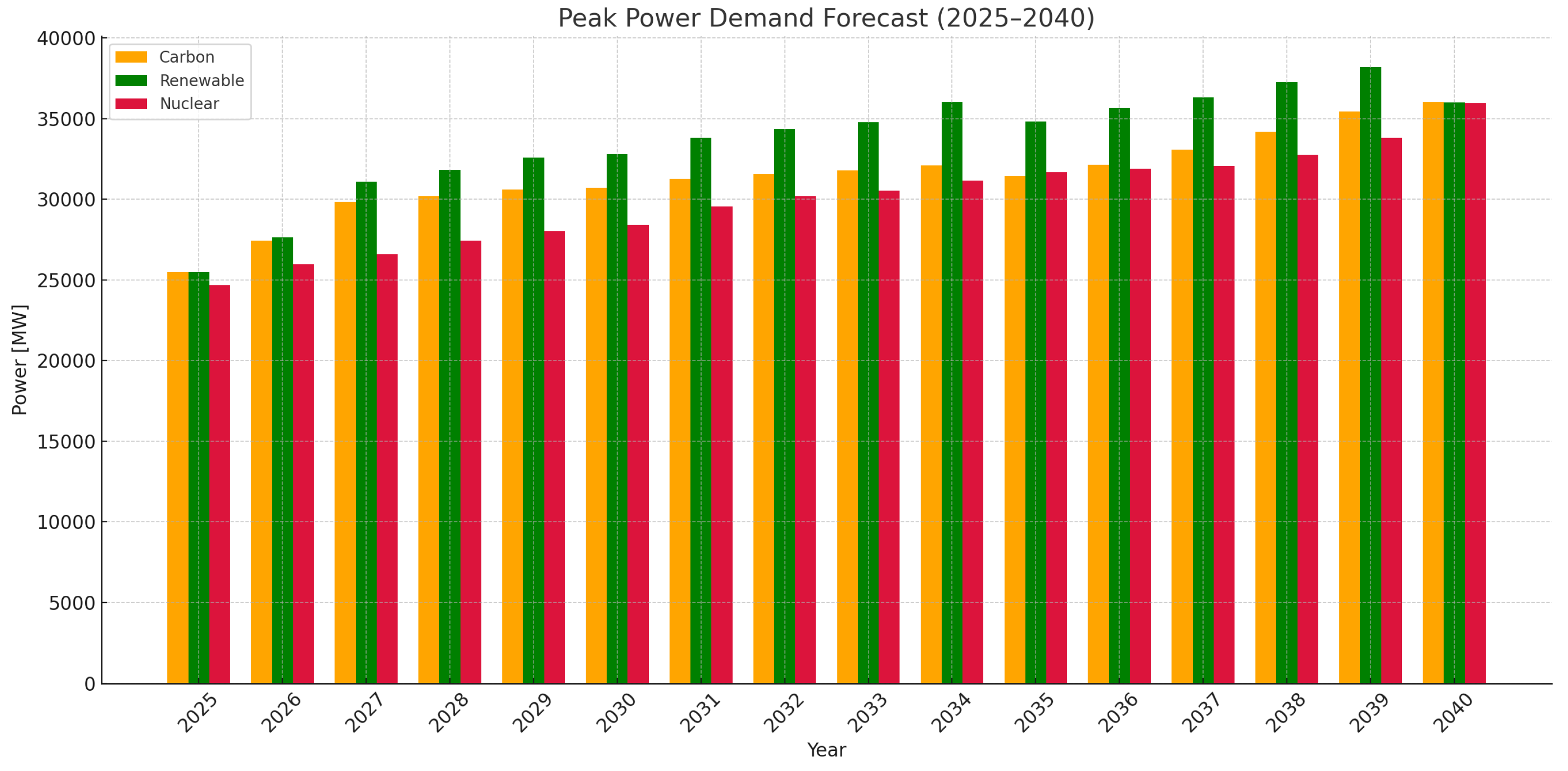
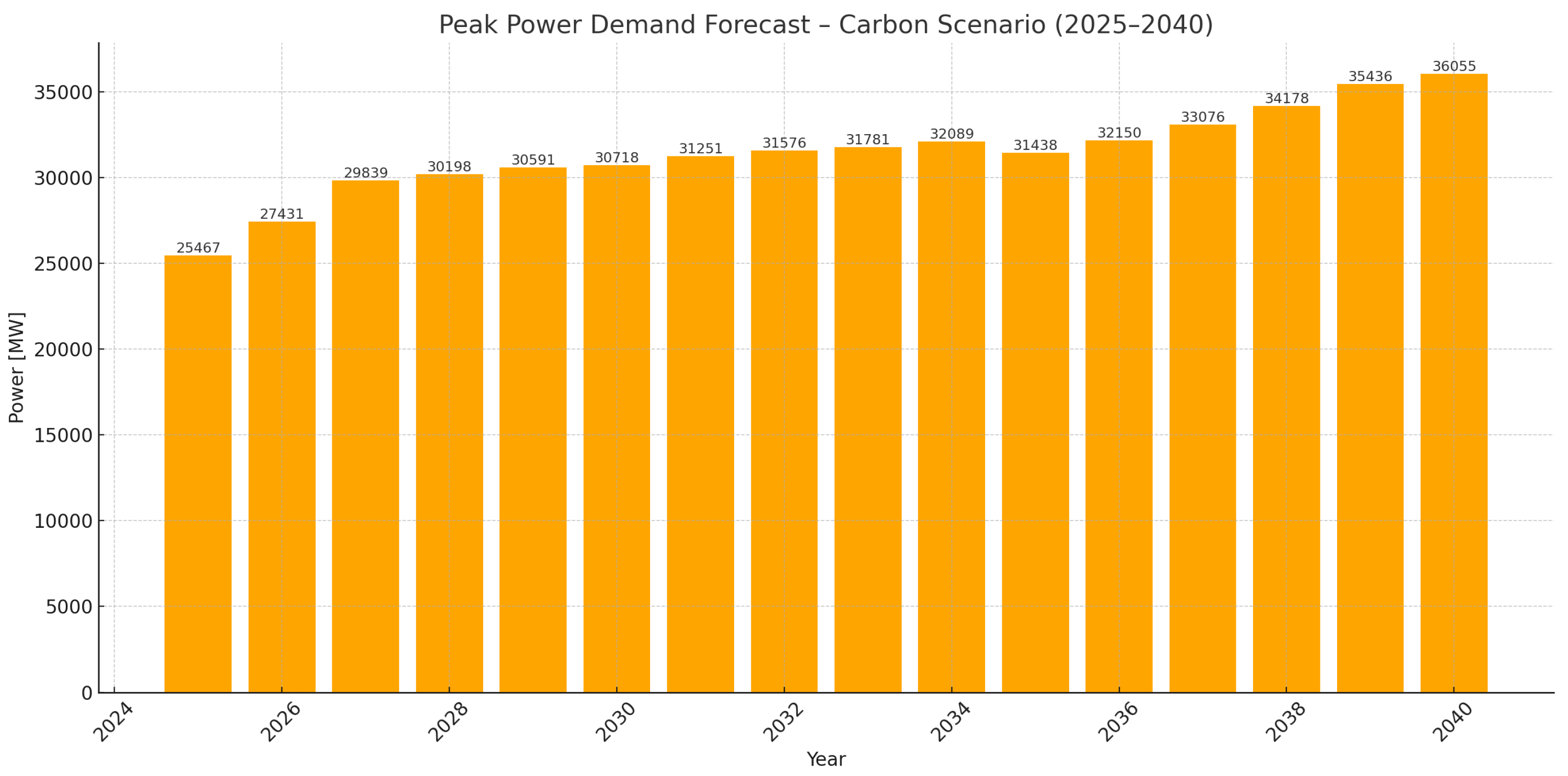
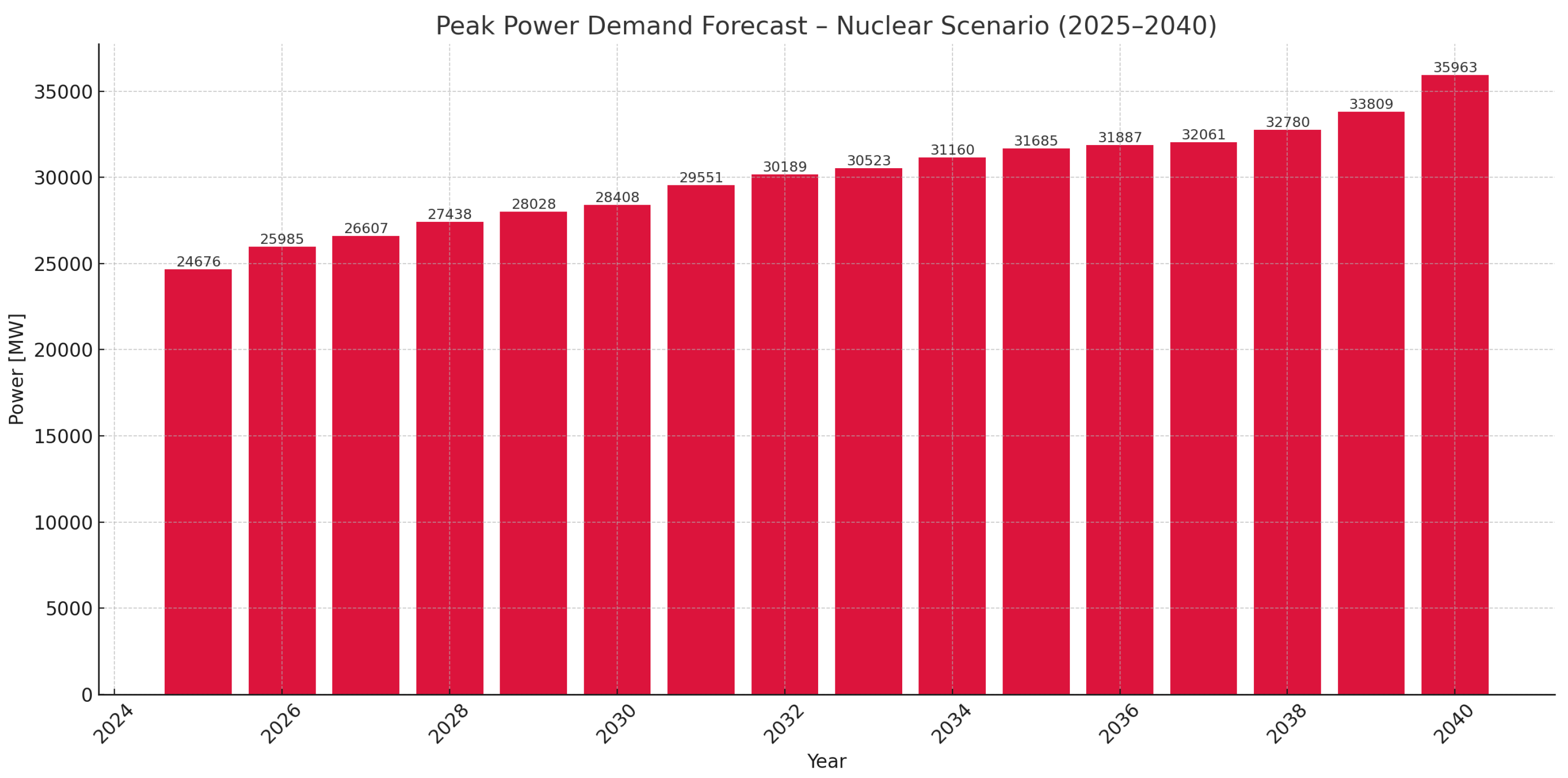
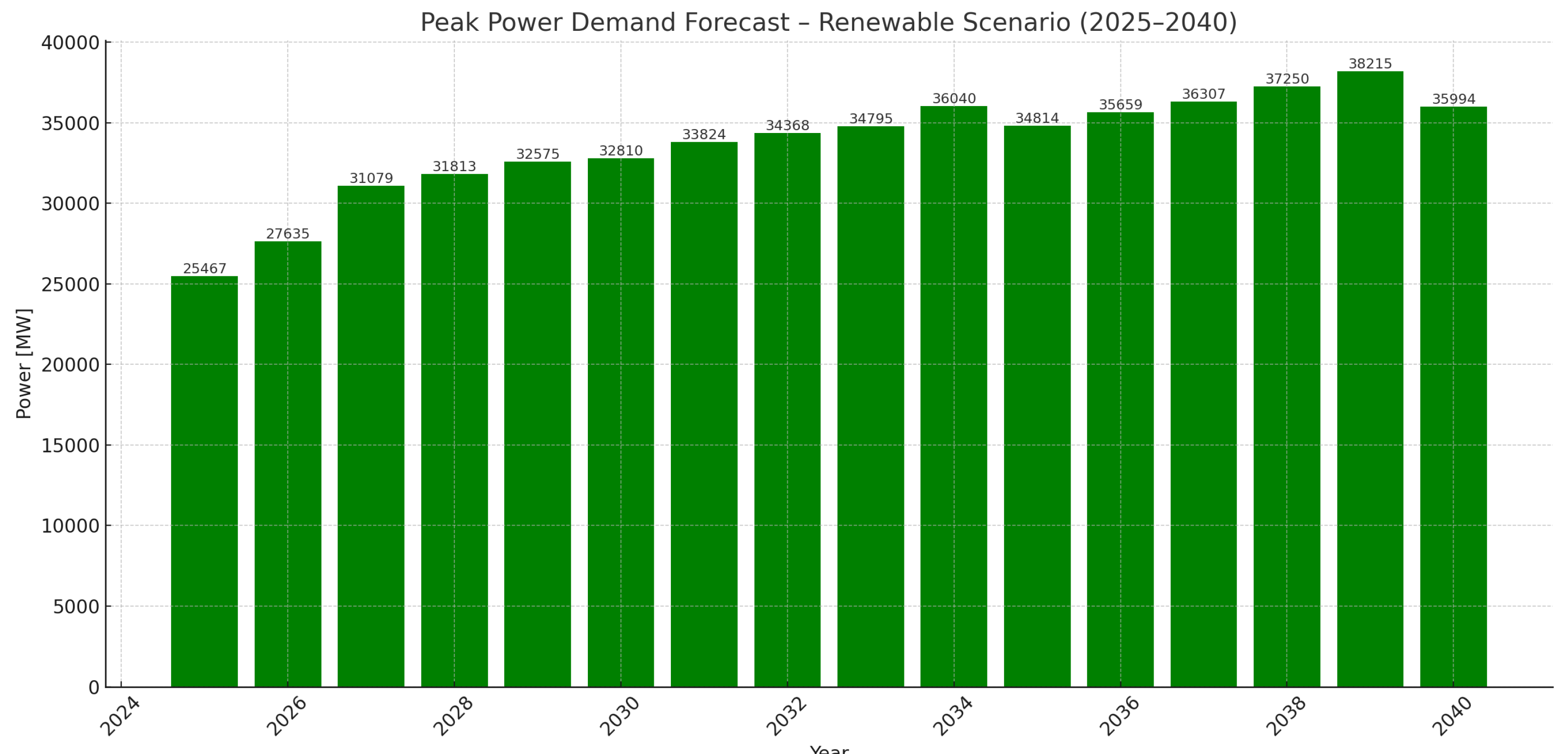
Three variants of the annual peaks in the power demand were obtained, depending on the adopted scenario regarding the annual gross energy demand. The results are illustrated collectively for the three scenarios in Figure 7 and for each scenario separately in Figure 8, Figure 9 and Figure 10. Additionally, in Figure 8, Figure 9 and Figure 10, the obtained numerical values [MW] are plotted above the annual forecast bars.

4. Discussion

Planning the long-term development of the national power system requires precise forecasts of the peak power demand. A key aspect of these forecasts is the selection of an appropriate modeling method that takes into account the complexity of the phenomena occurring in the energy sector.
1.
This paper proposes the use of a simplified forecasting model based on a modified Prigogin logistic equation. This model is based on deterministic chaos theory and describes the development of the population (or analogously, the power system) as a nonlinear system far from equilibrium. Equation (4) allows us to take into account phenomena such as a sudden increase in the demand, bifurcations and potential chaotic states in the power system. This model was tested and adapted to forecast the long-term peak power demand in Poland, using parameters such as the annual growth factor ( R = 0.3938 ) and the asymptotic limit of the system’s development ( K = 0.7688 ).
2.
Based on strategic documents, such as the annex to PEP2040 [44] and scenario analyses up to 2040 [46], several gross energy demand paths were identified. The variants predicted an annual gross energy demand in Poland of 230–235 TWh in 2040 with a corresponding increase in the peak power demand from 28.7 GW (2024) to over 34.5 GW (2040). The Prigogin model allowed for the dynamic linking of energy consumption with the power demand by taking into account the average annual load factor ( A L F ), in accordance with the relation in (3). The use of this relation allowed for the transformation of energy consumption forecasts (e.g., for RES, nuclear energy and coal energy scenario variants) into the power demand using A L F scenarios (e.g., increasing system management efficiency).
3.
Compared to complex models such as the WEM, PRIMES and POLES, the proposed Prigogin method offers several significant advantages:
  • Low computational complexity—the model does not require advanced IT infrastructure, which makes it accessible to institutions with limited resources.
  • Speed of implementation—fast calibration and scenario generation.
  • The ability to analyze chaos and bifurcations—a unique feature of the Prigogin model allows for the assessment of unpredictable dynamic changes (e.g., sudden increases in the demand due to weather extremes).
  • Consistency with real historical data—as shown in Table 4 in this article, the model achieved high consistency with PSE data for the years 2014–2024.
4.
A disadvantage of the Prigogin model is its limited ability to integrate the consideration of sectoral policies, technologies and prices, with the ability to do so being a strong point of models such as the PRIMES or WEM. However, when using hybrid models (i.e., the Prigogin model + scenarios from the POLES or PRIMES), it is possible to obtain a simultaneously comprehensive and effective decision-making tool.
5.
The adoption of the simplified Prigogin model in the context of planning the development of the national power system brings the following benefits:
  • The transparency and interpretability of the results, which facilitates communication with political and social stakeholders.
  • The possibility to quickly test alternative development paths, e.g., the accelerated electrification of transport or changes to the A L F .
  • Cost-effectiveness—with low computational costs and required amounts of input data, it is possible to obtain solid forecasts for investment planning purposes.
According to the author, the Prigogin model, although simplified, is a valuable tool supporting the process of peak power demand planning in Poland. This article attempts to prove that, in combination with the use of realistic scenarios for the gross energy demand and ALF analysis, this model allows for the formulation of effective strategies for the development of the power system until 2040, and its supplementation with complex models (PRIMES, POLES) can provide a basis for an integrated decision support system in the energy sector.

5. Conclusions

Based on the research presented in this article, the following key conclusions can be drawn:
1.
The Effectiveness of the Simplified Forecasting Models:
This study demonstrates that, despite their limitations compared to complex simulation tools (such as the PRIMES, WEM or POLES), simplified models based on the Prigogine equation can provide fast, low-cost and sufficiently accurate long-term forecasts of the peak power demand. These models are particularly valuable when detailed input data is unavailable or when rapid assessments are needed.
2.
The Application of the Prigogine Equation:
A modified Prigogine equation, derived from the classical logistic model developed by Verhulst, was adapted to model the annual average load factor ( A L F ) of the Polish power system. The key parameters included the following:
  • R—the growth rate coefficient (optimized to 0.3938);
  • K—the saturation level or development ceiling for the A L F (determined to be 0.7688 based on historical trend extrapolation).
The model demonstrated very good historical fit:
  • The Mean Absolute Percentage Error (MAPE) for the A L F forecast was 0.76 % ;
  • The MAPE for the peak power demand forecast (validation forecast for 2014–2024) was 1.85 % .
3.
Gross Electricity Demand Scenarios:
Three long-term electricity demand scenarios for Poland through 2040 were considered (coal-based, nuclear and RES-driven), based on institutional forecasts (e.g., PSE, FNEZ). The Prigogine equation was used to predict future ALF values, which were then combined with energy demand forecasts to calculate peak power using the formula (3).
4.
Forecast Results up to 2040:
Depending on the adopted energy demand scenario, the demand differed:
  • In the RES-based scenario, the peak power demand could reach nearly 40 GW by 2040;
  • In the coal-based scenario, the demand would be slightly lower, around 38–39 GW.
  • These results indicate growing strain on Poland’s power system due to economic development and electrification trends.
5.
Strategic Implications:
  • The Prigogine equation has proven to be a valuable and flexible tool for long-term energy planning, especially under uncertainty.
  • It allows for continuous recalibration and quick adjustments to changing economic or policy conditions.
  • The model supports strategic decision-making and complements the use of more detailed simulations, especially in the early planning phases.
  • Its theoretical foundation in non-equilibrium thermodynamics aligns with the complex, dynamic nature of modern power systems.

Funding

This research received no external funding.

Data Availability Statement

The original contributions presented in this study are included in the article; further inquiries can be directed to the author.

Conflicts of Interest

The author declares no conflicts of interest.

References

  1. Popławski, T. Theory and Practice in Planning the Development and Operation of Power Systems; Selected Aspects; Czestochowa University of Technology Publishing House: Czestochowa, Poland, 2013. (In Polish) [Google Scholar]
  2. International Energy Agency. Global Energy and Climate Model. Documentation. 2024. Available online: https://www.iea.org/reports/world-energy-model (accessed on 15 April 2025).
  3. International Energy Agency. World Energy Outlook 2023. 2023. Available online: https://www.iea.org/reports/world-energy-outlook-2023 (accessed on 15 April 2025).
  4. E3MLab/ICCS. PRIMES Model. Available online: https://e3modelling.com/modelling-tools/primes/ (accessed on 15 April 2025).
  5. European Commission. Impact Assessment Accompanying the 2030 Climate Target Plan. 2020. Available online: https://eur-lex.europa.eu/legal-content/EN/TXT/?uri=CELEX:52020SC0176 (accessed on 15 April 2025).
  6. IEA-ETSAP. Energy System Models: PRIMES, POLES, TIMES—A Comparative Overview. Available online: https://iea-etsap.org (accessed on 15 April 2025).
  7. Criqui, P.; Mima, S.; Kitous, A.; Hamdi-Cherif, M. The POLES Energy Model: Technical Overview. CNRS–LEPII and Enerdata. 2015. Available online: https://www.enerdata.net/solutions/poles-model.html (accessed on 15 April 2025).
  8. TU Wien—Energy Economics Group. Green-X Model Overview. Available online: https://www.green-x.at (accessed on 15 April 2025).
  9. Schöniger, F.; Resch, G.; Suna, D.; Widhalm, P.; Totschnig, G.; Pardo Garcia, N.; Hasengst, F.; Formayer, H.; Maier, P.; Leidinger, D. The Impact of Climate Change on Electricity Demand and Supply Profiles in Europe Until 2100. 2024. Available online: https://ssrn.com/abstract=4978968 (accessed on 20 May 2025).
  10. Chudy, M.; Karmakar, S.; Wu, W.B. Long-term prediction intervals of economic time series. arXiv 2020, arXiv:2002.05384. [Google Scholar] [CrossRef]
  11. Pindyck, R.S.; Santen, N.P. Uncertainty in forecasts of long-run economic growth. Proc. Natl. Acad. Sci. USA 2018, 115, 5409–5414. [Google Scholar] [CrossRef]
  12. Weron, R. Modeling and Forecasting Prices in the Electricity Market; Scientific and Technical Publishing House: Warsaw, Poland, 2006. (In Polish) [Google Scholar]
  13. Tsai, P.-H.; Berleant, D.; Segall, R.S.; Aboudja, H.; Batthula, V.J.R.; Duggirala, S.; Howell, M. Quantitative technology forecasting: A review of trend extrapolation methods. arXiv 2024, arXiv:2401.02549. [Google Scholar] [CrossRef]
  14. Hao, J.; Liu, F. Improving long-term multivariate time series forecasting with a seasonal-trend decomposition-based 2-dimensional temporal convolution dense network. Sci. Rep. 2024, 14, 1689. Available online: https://www.nature.com/articles/s41598-024-52240-y (accessed on 10 May 2025). [CrossRef] [PubMed]
  15. Abdelkader, M.; Benbouzid, M.; El Bouzidi, Y.; El Amrani, M.; El Fadili, M.E.H. Modeling and forecasting historical volatility using econometric models: A comparative study. J. Risk Financ. Manag. 2024, 17, 300. [Google Scholar] [CrossRef]
  16. Shah, D.; Thaker, M. A review of time series forecasting methods. Int. J. Res. Anal. Rev. 2024, 11, 749. Available online: https://www.researchgate.net/publication/379862462_A_Review_of_Time_Series_Forecasting_Methods (accessed on 10 May 2025).
  17. Chauvet, M.; Piger, J. Predicting recessions: A new approach for identifying leading indicators and forecast combinations. International Monetary Fund. 2016. Available online: https://www.imf.org/en/Publications/WP/Issues/2016/12/31/Predicting-Recessions-A-New-Approach-for-Identifying-Leading-Indicators-and-Forecast-25288 (accessed on 10 May 2025).
  18. Garnitz, J.; Lehmann, R.; Wohlrabe, K. Forecasting GDP All over the World Using Leading Indicators Based on Comprehensive Survey Data. CESifo Working Paper No. 7691. 2019. Available online: https://www.econstor.eu/handle/10419/201917 (accessed on 10 May 2025).
  19. Groen, J.J.J.; Kapon, G.A. A comparison of monthly global indicators for forecasting growth. Int. J. Forecast. 2021, 37, 1276–1295. [Google Scholar] [CrossRef]
  20. Lehmann, R.; Wohlrabe, K. The forecasting power of the ifo Business Survey. J. Bus. Cycle Res. 2022, 18, 1–21. [Google Scholar] [CrossRef]
  21. Xie, J. Identifying Optimal Indicators and Lag Terms for Nowcasting Models. International Monetary Fund. 2023. Available online: https://www.imf.org/en/Publications/WP/Issues/2023/03/02/Identifying-Optimal-Indicators-and-Lag-Terms-for-Nowcasting-Models-530335 (accessed on 10 May 2025).
  22. Atesongun, A.; Gulsen, M. A hybrid forecasting structure based on ARIMA and artificial neural network models. Appl. Sci. 2024, 14, 7122. [Google Scholar] [CrossRef]
  23. Bulut, C.; Hudaverdi, B. Hybrid approaches in financial time series forecasting: A stock market application. EKOIST J. Econom. Stat. 2022, 37, 53–68. [Google Scholar] [CrossRef]
  24. Smyl, S.; Dudek, G.; Pełka, P. ES-dRNN: A hybrid exponential smoothing and dilated recurrent neural network model for short-term load forecasting. arXiv 2021, arXiv:2112.02663. [Google Scholar] [CrossRef]
  25. Zhong, Y.; Cheng, Q.; Qin, L.; Xu, J.; Wang, H. Hybrid deep learning for AI-based financial time series prediction. J. Econ. Theory Bus. Manag. 2024, 1, 27–35. [Google Scholar] [CrossRef]
  26. Peujio Fozap, F.M. Hybrid machine learning models for long-term stock market forecasting: Integrating technical indicators. J. Risk Financ. Manag. 2025, 18, 201. [Google Scholar] [CrossRef]
  27. Dai, S.; Meng, F.; Dai, H.; Wang, Q.; Chen, X. Electrical peak demand forecasting: A review. arXiv 2021, arXiv:2108.01393. [Google Scholar]
  28. International Energy Agency (IEA). Energy Technology Perspectives. 2020. Available online: https://www.iea.org (accessed on 18 May 2025).
  29. ENTSO-E. Ten-Year Network Development Plan (TYNDP). 2023. Available online: https://tyndp.entsoe.eu (accessed on 18 May 2025).
  30. Verhulst, P.F. Notice sur la loi que la population poursuit dans son accroissement. Corresp. Math. Phys. 1838, 10, 113–121. [Google Scholar]
  31. Anokye, M.; Donkoh, E.K.; Ofori, M.F.; Adom-Konadu, A. Full Delay Logistic Population Model with Sustainable Harvesting. J. Appl. Math. 2022, 2022, 6777827. [Google Scholar] [CrossRef]
  32. Ornelas, A.; Delgado-Vences, F.; Morales-Bojórquez, E.; Cruz-Escalona, V.H.; Marín-Enríquez, E.; Hernández-Camacho, C.J. Modeling the Biological Growth with a Random Logistic Differential Equation. Environ. Ecol. Stat. 2023, 30, 233–260. [Google Scholar] [CrossRef]
  33. García-Algarra, J.; Galeano, J.; Pastor, J.M.; Iriondo, J.M.; Ramasco, J.J. Rethinking the Logistic Approach for Population Dynamics of Mutualistic Interactions. arXiv 2013, arXiv:1305.5411. [Google Scholar] [CrossRef]
  34. Marchetti, C.; Meyer, P.S.; Ausubel, J.H. Human Population Dynamics Revisited with the Logistic Model: How Much Can Be Modeled and Predicted? Technol. Forecast. Soc. Change 1996, 52, 1–12. [Google Scholar] [CrossRef]
  35. Ershkov, S.V. Logistic Equation of Human Population Growth (Generalization to the Case of Reactive Environment). viXra Quant. Biol. 2011, 1103.0085v1. Available online: https://vixra.org/abs/1103.0085 (accessed on 18 May 2025).
  36. Hernando, A.; Plastino, A. Scale-Invariance Underlying the Logistic Equation and Its Social Applications. arXiv 2012, arXiv:1204.2422. [Google Scholar] [CrossRef]
  37. Méndez, V.; Assaf, M.; Campos, D.; Horsthemke, W. Stochastic Dynamics and Logistic Population Growth. arXiv 2015, arXiv:1506.01137. [Google Scholar] [CrossRef] [PubMed]
  38. Rodrigo, M.; Zulkarnaen, D. Mathematical Models for Population Growth with Variable Carrying Capacity: Analytical Solutions. Mathematics 2022, 2, 466–479. [Google Scholar] [CrossRef]
  39. Miranda, L.C.M.; Lima, C.A.S. On the Logistic Modeling and Forecasting of Evolutionary Processes: Application to Human Population Dynamics. Technol. Forecast. Soc. Change 2010, 77, 699–711. [Google Scholar] [CrossRef]
  40. Petroni, N.C.; De Martino, S.; De Siena, S. Logistic and Q-Logistic Models in Population Dynamics: General Analysis and Exact Results. arXiv 2020, arXiv:2004.10478. [Google Scholar]
  41. Prigogine, I.; Stengers, I. From Chaos to Order; State Publishing Institute: Warsaw, Poland, 1990. (In Polish) [Google Scholar]
  42. Dobrzańska, I.; Dąsal, K.; Łyp, J.; Popławski, T.; Sowiński, J. Forecasting in the Power Industry; Selected Issues; Częstochowa University of Technology Publishing House: Częstochowa, Poland, 2002. (In Polish) [Google Scholar]
  43. Baczyński, D.; Parol, M.; Piotrowski, P. Contemporary Problems of Forecasting in the Power Industry; Selected Issues; Warsaw University of Technology Publishing House: Warsaw, Poland, 2020. (In Polish) [Google Scholar]
  44. Ministry of Climate and Environment. Energy Policy of Poland Until 2040. Warsaw. 2021. Available online: https://www.gov.pl/web/klimat/polityka-energetyczna-polski (accessed on 18 May 2025). (In Polish)
  45. Polish Power Grids, S.A. Assessment of Resource Adequacy at the National Level 2025–2040, November 2024. Available online: https://www.pse.pl/-/publikacja-raportu-zgodnie-z-art-15-i-ustawy-prawo-energetyczne?safeargs=696e686572697452656469726563743d74727565 (accessed on 18 May 2025). (In Polish).
  46. Stryjecki, M. Forecast of the Structure of the Polish Power System Until 2040; Coal, Nuclear, RES Scenario; Foundation for Sustainable Energy: Warsaw, Poland, 2019. (In Polish) [Google Scholar]
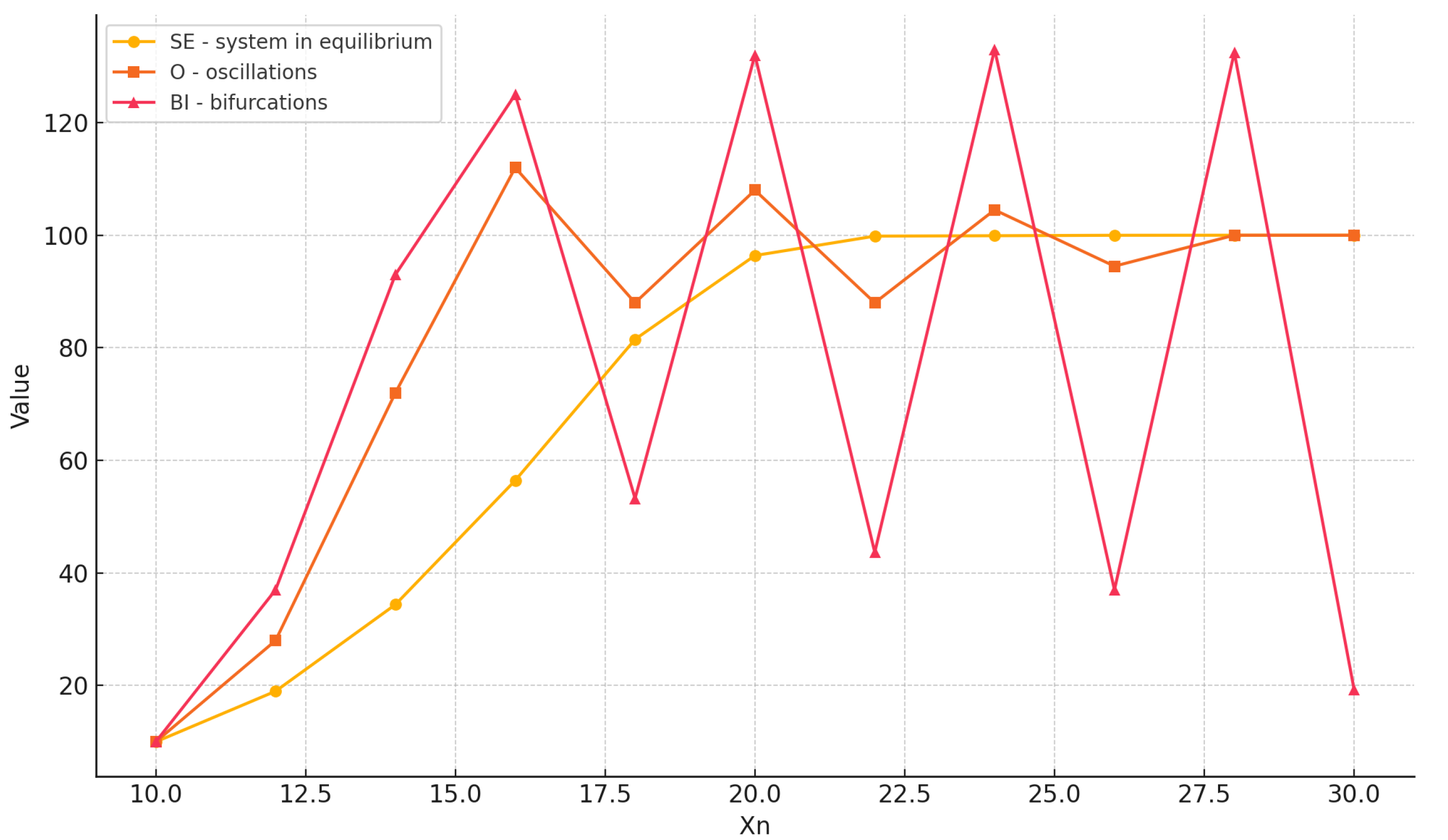
Figure 1. The process modeled by the Prigogin equation in a state of equilibrium (SE), with convergence to K with oscillations (O) and with bifurcation (BI) at the development level K = 100. Source: Author’s own study based on [1,42,43].
Energies 18 03472 g001
Figure 2. The process modeled by the Prigogin equation in a state of striving for balance (SB), with a jump to K in the first few steps (AB) and in chaos (CH) at the development level K = 100. Source: Author’s own study based on [1,42,43].
Energies 18 03472 g002
Figure 3. The average annual load factor ( A L F ) determined for the Polish power system for the years 1985 to 2024. Source: Author’s own study.
Energies 18 03472 g003
Figure 4. Long-term forecast of a highly probable volatility range for the A L F up to 2044. Source: Author’s own study.
Energies 18 03472 g004
Figure 5. Gross electricity demand scenarios for Poland until 2040. Source: Author’s own study.
Energies 18 03472 g005
Figure 6. Gross electricity demand scenarios for Poland until 2040. Source: Own work based on [46].
Energies 18 03472 g006
Figure 7. Forecast of peak power demand for Poland until 2040 with three variants of gross electricity demand in coal energy, RES and nuclear energy scenarios. Source: Author’s own study.
Energies 18 03472 g007
Figure 8. Forecast of peak power demand for Poland until 2040 for coal variant of gross electricity demand. Source: Author’s own study.
Energies 18 03472 g008
Figure 9. Forecast of peak power demand for Poland until 2040 for nuclear variant of gross electricity demand. Source: Author’s own study.
Energies 18 03472 g009
Figure 10. Forecast of peak power demand for Poland until 2040 for RES variant of gross electricity demand. Source: Author’s own study.
Energies 18 03472 g010
Table 1. Comparison of simple and advanced forecasting models. Source: Author’s own study, based on [12,27,28,29].
FeatureSimplified Forecasting ModelsAdvanced Forecasting ModelsSource
ComplexityLow—simple equations, limited number of variablesHigh—many variables, complex model structure[12,28]
Input data requirementsLow—historical data, fundamental indicatorsHigh—detailed sector, technology and demographic data[27,29]
Cost of and time taken for implementationLow cost, fast implementationHigh cost, time-consuming[28]
Example methodsLinear regression, trend extrapolation, individual indicatorsBottom-up simulations, econometric models with dynamic structures, AI/ML[12,28]
Scenario flexibilityLimited—difficulty in analyzing the impact of policy or technology changesHigh—possibility of creating different scenarios (e.g., considering impact of electromobility)[27,28]
Transparency of resultsHigh—easy interpretationLow—results often require advanced analysis[27]
Long-term accuracyMedium to low—high sensitivity to external changesHigh—more resistant to variability of conditions[28,29]
ApplicationsDeveloping countries, rapid analysis, early planning stagesStrategic planning, large-scale power systems[12,28]
Table 2. Validation forecast results for the average A L F for the years 2014 to 2024. Source: Author’s own study.
Year ALF
[-]
ALF Forecast
[-]
MAPE
[%]
20140.70990.70970.02
20150.71090.71070.02
20160.71100.71170.09
20170.71520.71270.35
20180.71800.71370.59
20190.71860.71470.54
20200.72080.71560.72
20210.72610.71651.32
20220.72780.71731.44
20230.72840.71821.40
20240.73220.71901.80
Table 3. Long-term electricity demand scenarios for Poland until 2040. Source: Own work based on [44,45,46].
ScenarioSourceDemand in 2040 [TWh]
APEP 2040 (2021) 1230
BScenario 3 2244
CFNEZ 3235
DPSE S.A. 4243
1 The official government forecast assumes an average annual growth rate of 1.7% in 2018–2040 [44]. 2 An update (2023) to PEP 2040, taking into account the intensive electrification of transport and heating [44]. 3 Considering three variants of the energy mix, assuming different shares of energy sources [46]. 4 Taking into account the sum of the base demand and sectoral demands due to heat pumps, electrode boilers, electromobility, data centers and hydrogen production [45].
Table 4. Validation forecast of peak power demand for Poland for years 2014 to 2024. Source: Author’s own study.
Year P r , real
 [MW]
P r , val
 [MW]
MAPE
[%]
201425,53525,479.00.22
201525,10125,637.02.14
201625,54625,859.91.23
201726,23126,232.60.01
201826,44826,549.00.38
201926,50426,861.91.35
202026,79926,209.42.20
202127,61726,679.63.39
202227,29626,944.91.29
202327,32626,951.71.37
202428,66026,717.16.78
Disclaimer/Publisher’s Note: The statements, opinions and data contained in all publications are solely those of the individual author(s) and contributor(s) and not of MDPI and/or the editor(s). MDPI and/or the editor(s) disclaim responsibility for any injury to people or property resulting from any ideas, methods, instructions or products referred to in the content.