1. Introduction
The rapid global adoption of renewable energy and electric vehicles (EVs) presents both opportunities and challenges for modern power systems [
1]. While wind and solar generation capacity has grown exponentially, their inherent intermittency and spatiotemporal variability complicate grid planning and operation, necessitating high-precision forecasting methods to mitigate uncertainty. Concurrently, EV adoption introduces aggregated charging loads with distinct temporal patterns, further straining distribution networks. Compounding these challenges, carbon pricing frameworks have emerged as critical policy tools to incentivize decarbonization, yet existing mechanisms often lack the flexibility to adapt to dynamic emission reduction targets [
2]. This trend has forced the comprehensive upgrade of the distribution network planning concepts and methods, and it is urgent to build a new planning system that adapts to the high proportion of renewable energy access. Modern distribution network planning has evolved into a multidimensional, multi-stage system of engineering, and its core tasks can be decomposed into power supply side collaborative planning and grid planning [
3]. Power planning is no longer limited to the site selection and capacity determination of traditional thermal power plants and gas turbines. Still, it needs to comprehensively consider the penetration rate of fluctuating power sources such as wind and solar power, the clustering effect of distributed energy, and the optimal configuration of flexible resources such as charging piles and energy storage power stations [
4]. The planning focus has shifted from simple capacity matching to both “controllability” and “flexibility” to ensure that the system can still operate stably when the output of renewable energy fluctuates greatly [
5]. Grid planning improves the carrying capacity and fault self-healing ability of the existing network through line capacity expansion and intelligent segmented switch deployment. For application scenarios such as emerging industrial parks, a new topology is constructed, and access space for technologies such as energy storage is reserved [
6,
7,
8]. From passively adapting to load growth to actively guiding energy transformation and upgrading, the maximum absorption of renewable energy is achieved while ensuring power supply reliability.
In the context of new power systems, the volatility and spatiotemporal uncertainty of renewable energy represented by photovoltaic and wind power have significantly increased the planning difficulty of distribution networks in terms of grid optimization, operation scheduling, and improvement of absorption capacity. High-precision renewable energy output forecasts (such as wind speed and solar irradiance) are the core inputs for planning decisions, and their reliability is directly related to the economic performance and stability of the power system [
9]. Existing prediction methods primarily fall into three categories: ① Traditional statistical models: These mainly include the primary approach, which involves time series forecasting based on the auto-regressive moving average (ARMA) model, and hybrid prediction methods based on seasonal and trend decomposition using LOESS (STL) decomposition and simple exponential smoothing (SES) [
10,
11]. This type of method achieves trend fitting through linear assumptions and periodic decomposition, but it is not capable of capturing nonlinear characteristics (such as power mutations caused by extreme weather) and is difficult to handle multivariate coupling relationships; ② Traditional machine learning methods: Techniques such as support vector machines (SVM) [
12], random forests, and gradient boosting decision trees (GBDT) [
13] can improve nonlinear fitting through feature engineering. However, they suffer from inherent limitations in temporal dependency modeling, and the manual feature construction process may introduce subjective biases, leading to high computational complexity and poor real-time performance. ③ Deep learning models: These include convolutional neural networks (CNN) [
14], transformer [
15], and long short-term memory (LSTM). Although LSTM excels in temporal modeling, standalone LSTM algorithms [
16] exhibit limited capability in modeling non-stationary signals (e.g., abrupt changes in solar irradiance or wind speed). Moreover, traditional decomposition methods like empirical mode decomposition (EMD) may obscure the physical interpretability of subsequences, further compromising prediction reliability.
As the penetration rate of EV charging load in the power system continues to rise, its agglomeration characteristics in time and space dimensions have a profound impact on the planning and operation of the distribution network [
17]. Scientific modeling and in-depth analysis are needed at the system level to ensure the safety, reliability, and economy of the power grid [
18]. According to the differences in charging behavior, EV users can be divided into two categories [
19]: slow-charging users (mainly private cars, charging at fixed time periods at night in residential areas) and fast-charging users (mainly taxis, relying on centralized fast-charging stations for high-frequency short-term charging). Since the access location of centralized fast-charging stations directly affects the distribution of the distribution network power flow, their site selection and capacity determination must be based on refined load forecasting. Existing EV load forecasting methods mainly include the following: ① Probabilistic modeling method: constructing charging demand probability distribution based on historical data (such as Monte Carlo simulation) [
20,
21]. It has high computational efficiency but tends to ignore user dynamic behavior. ② Travel behavior analysis method: inferring load demand through the transmission relationship and transmission rules between user activity chains combined with a dynamic traffic distribution model [
22]. Although it can reflect individual behavior logic, it is difficult to extend to the entire user group. ③ Data-driven method: using travel trajectory data for data mining and integrated modeling to predict load results [
23,
24]. Although this method has strong timeliness, it relies on high-cost data collection systems. Current research mostly integrates EV loads and lacks modeling of differentiated charging modes for slow-charging/fast-charging users, resulting in prediction results that are difficult to support differentiated distribution network planning needs.
As the types of loads such as distributed energy and electric vehicles continue to increase, distribution network planning has begun to shift from considering single elements such as power supply reliability and flexibility [
25] and network losses [
26] to a new distribution network that integrates multiple elements such as distributed power sources and electric vehicles. Reference [
27] proposed a joint planning method for electric vehicle charging stations and distribution networks, which considered the demand characteristics of charging stations. Reference [
28] incorporated distributed power sources into distribution network planning and proposed a distribution network planning method based on probabilistic flow, using a probabilistic model to deal with the large number of uncertainties brought about by wind power and photovoltaic access. To meet the demand for maximizing renewable energy accommodation, distribution network planning must also account for the impact of carbon emissions to achieve sustainable development. Reference [
29] incorporated carbon emission costs into distribution network planning to reduce greenhouse gas emissions. However, the carbon emission model employed was overly simplistic and failed to consider the positive role of carbon trading markets in incentivizing emission reductions. Reference [
30] introduced a carbon trading mechanism by incorporating the carbon price as a fixed parameter within the carbon cost objective of the operational model. However, this approach overlooked the temporal variability of carbon prices and the tradability of carbon allowances, resulting in a relatively rigid representation of the carbon market. Consequently, it failed to adequately reflect the dynamic nature and complexity of real-world carbon trading mechanisms. To address such limitations, Reference [
31] presented a traditional tiered carbon trading mechanism alongside a carbon emission calculation model. In this framework, the carbon price increases stepwise with the quantity of emission allowances purchased, strengthening cost signals for higher emissions. Nevertheless, its pricing structure remains static and lacks adaptability to real-time emission dynamics. Building upon this, Reference [
32] improved the model by introducing a carbon price growth rate, enabling the carbon price to increase progressively across emission stages. This enhancement not only added flexibility to the pricing mechanism but also improved its effectiveness in incentivizing emission reductions and aligning carbon pricing with actual emission behaviors.
The rapid integration of renewable energy and EVs introduces critical challenges for power systems, including renewable intermittency, spatially concentrated EV charging loads, and inefficient carbon pricing mechanisms. Existing planning approaches often address these issues in isolation, failing to capture their interdependencies. This paper proposes a power grid planning method incorporating renewable energy and EV charging stations, leveraging a carbon pricing optimization mechanism. The key innovations include the following: (1) A renewable energy output prediction model considering climatic conditions is established to characterize the generation profiles of wind and solar power. (2) EV users are categorized into slow-charging and fast-charging users based on differences in charging behavior. Queueing theory and probabilistic forecasting models are employed to simulate travel patterns and analyze charging demand, thereby constructing an accurate charging station model. (3) A more flexible and incentive-driven carbon pricing optimization mechanism is introduced by incorporating carbon price growth rate adjustments, facilitating the efficient allocation of clean energy resources and dynamic optimization of carbon emission reduction pathways. Building upon this framework, an integrated power-traffic system co-planning model is formulated, minimizing total economic costs while accounting for renewable energy siting, EV charging station spatial distribution, and carbon trading expenses.
The remainder of this paper is structured as follows. In renewable energy forecasting,
Section 2 adopts a hybrid strategy combining complete ensemble empirical mode decomposition with adaptive noise (CEEMDAN) and multi-channel LSTM networks, significantly enhancing the accuracy and robustness of wind and photovoltaic power predictions. This provides more reliable data support for subsequent optimization. In
Section 3, the heterogeneity of user behavior is rigorously addressed for EV load modeling: queueing theory models are applied to fast-charging users, while probabilistic forecasting models are developed for slow-charging users. This granular approach improves the realism and specificity of charging load predictions, enabling more targeted charging station deployment. In
Section 4, the innovative integration of carbon price growth rate optimization enhances the flexibility and incentivization of the carbon pricing mechanism design. This promotes rational integration of distributed renewable energy and strengthens the system-wide carbon emission reduction capability. A case study based on the IEEE 33-node system is presented in
Section 5. The conclusion and discussion are provided in
Section 6 and
Section 7, respectively.
2. Renewable Energy Output Forecasting Based on CEEMDAN-LSTM
When describing the output characteristics of wind power and photovoltaic power, traditional methods usually directly use the light intensity curve and wind speed curve of a certain area for modeling. However, this method ignores the potential impact of environmental factors (such as temperature, humidity, air pressure, etc.) on wind power and photovoltaics, which may lead to deviations between the predicted results and the actual output. To more accurately characterize the output characteristics of renewable energy, this paper first conducts data-driven modeling of wind speed and light intensity based on historical data of multidimensional meteorological parameters, including wind speed, light intensity, temperature, humidity, and air pressure, and uses the CEEMDAN-LSTM algorithm for time series forecasting to improve the forecast accuracy and optimize the planning of renewable energy [
33].
2.1. CEEMDAN Decomposition
Ensemble empirical mode decomposition (EEMD) introduces random noise to the original data, performs EMD decomposition, and then takes the average [
34,
35]. The EEMD method can significantly alleviate the common modal aliasing problem in the EMD method by improving the decomposition process and improving the reliability of the decomposition results. The complete ensemble empirical mode decomposition (CEEMD) algorithm adds a large amount of Gaussian white noise with opposite phases and the same amplitude to the reconstructed signal based on EEMD. The decomposed and synthesized signal not only solves the problem of modal aliasing, but also keeps the residual noise value at a small level [
36].
The CEEMDAN algorithm is further optimized based on CEEMD, which enhances the stability and accuracy of decomposition. This method adds a limited number of adaptive white noises, which not only reduces the calculation time but also reduces the reconstruction error [
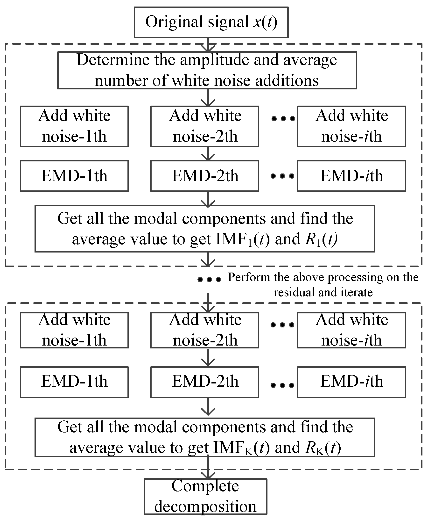
37]. The steps of CEEMDAN to process the meteorological data sequence are as follows:
- (1)
Assume that the white noise sequence vi(t) added for the i-th time obeys the normal distribution, the signal-to-noise ratio is represented by εk, and the operator of the k-th IMF generated by the EMD algorithm is Ek(*). The meteorological data sequence after the i-th noise is recorded as xi(t), and its calculation formula is as follows:
where
i represents the number of experiments conducted,
i = 1,2, …,
I, and
ε0 means the signal-to-noise ratio during the first decomposition stage.
- (2)
The EMD algorithm is applied to each noisy meteorological data sequence for decomposition processing, and then all modal components are summed and averaged to obtain the first modal component IMF1(t) and the residual component R1(t) = x(t) − IMF1(t).
- (3)
Continue to decompose R1(t) + ε1E1[vi(t)] once more to obtain the second IMF of CEEMDAN, namely,
where
ε1 means the signal-to-noise ratio during the second decomposition stage.
- (4)
The calculation of the (
k + 1)th IMF and residual component is the same as Step 3, expressed as follows:
- (5)
Until all residual components cannot be further decomposed, and the extreme value of the residual component is less than or equal to 2, the final residual component is as follows:
The signal time series is decomposed into the following:
According to the above steps, it is found that the appropriate signal-to-noise ratio can be selected through the coefficient
εk during decomposition; the reconstruction accuracy of the original meteorological data sequence is higher, and the calculation amount is less. The block diagram of CEEMDAN is shown in
Figure 1.
2.2. LSTM Prediction Model
The LSTM model consists of multiple gate structures, including an input gate, an output gate, and a forget gate, which work together to dynamically adjust the transmission and retention of information. As an improved form of a recurrent neural network, the LSTM model is good at capturing long-term dependencies and nonlinear trends in time series through the gating mechanism. Renewable energy is highly volatile and has time-series dependencies. LSTM can effectively alleviate the gradient vanishing problem and is suitable for processing wind speed and light intensity prediction tasks with multidimensional input. The structure of LSTM is shown in
Figure 2.
The core of the LSTM model is the process from the old memory state Ct−1 to the new memory state Ct. The algorithm uses a gate mechanism to memorize important information. The forgotten features in Ct−1 are obtained by the forget gate ft, which stops the forgotten features from entering the subsequent processing flow. ft is a vector with elements ranging from [0,1]. ⊗ indicates that there is a unit multiplication relationship between Ct−1 and ft. The internal operation process of the LSTM unit is as Equations (7)–(12).
The forget gate
ft is shown as follows:
The input gate
it is shown as follows:
The summarized status value
is shown as follows:
The new memory state
Ct is shown as follows:
In the formula, it is the input gate. Both it and ft are vectors with elements between [0,1] and are obtained by the input data xt and the previous hidden state ht−1 through the sigmoid activation function. xt and ht are obtained through the tanh activation function.
The output gate
Ot is shown as follows:
The updated output
ht is shown as follows:
In the formula, σ represents the sigmoid activation function, tanh represents the hyperbolic tangent function, Wf, Wi, Wc, and Wo are weight matrices, and bf, bi, bc, and bo are bias terms. The optimal model is obtained by optimizing the input data through multiple cycles.
2.3. Wind Power Output and Photovoltaic Output Forecast
This paper selects relevant historical data from a certain place as the test dataset. The time resolution of this data set is 1 h, and it contains five key meteorological indicators: wind speed, light intensity, temperature, humidity, and air pressure. Although solar irradiance is the most direct input to determine the photovoltaic output prediction, other meteorological parameters play an important synergistic role in the CEEMDAN-LSTM model. Temperature directly affects the conversion efficiency of photovoltaic cells. The power output of silicon photovoltaic cells decreases with the increase in temperature. High humidity will increase the content of water vapor in the atmosphere and reduce the actual solar radiation intensity reaching photovoltaic modules. The change in air pressure is closely related to the weather system, which affects the scattering and absorption of solar radiation due to large air tightness. Wind speed affects the temperature of photovoltaic modules through a cooling effect. Higher wind speed helps to reduce the temperature of modules and improve power generation efficiency. Therefore, we retain the five-dimensional meteorological characteristics in the CEEMDAN-LSTM framework, so that the network can capture the nonlinear interaction between the parameters. This multi-parameter collaborative prediction method is more accurate than the traditional model that simply depends on the light intensity, especially in complex weather conditions, which can provide more reliable prediction results. The same is true for wind power output prediction.
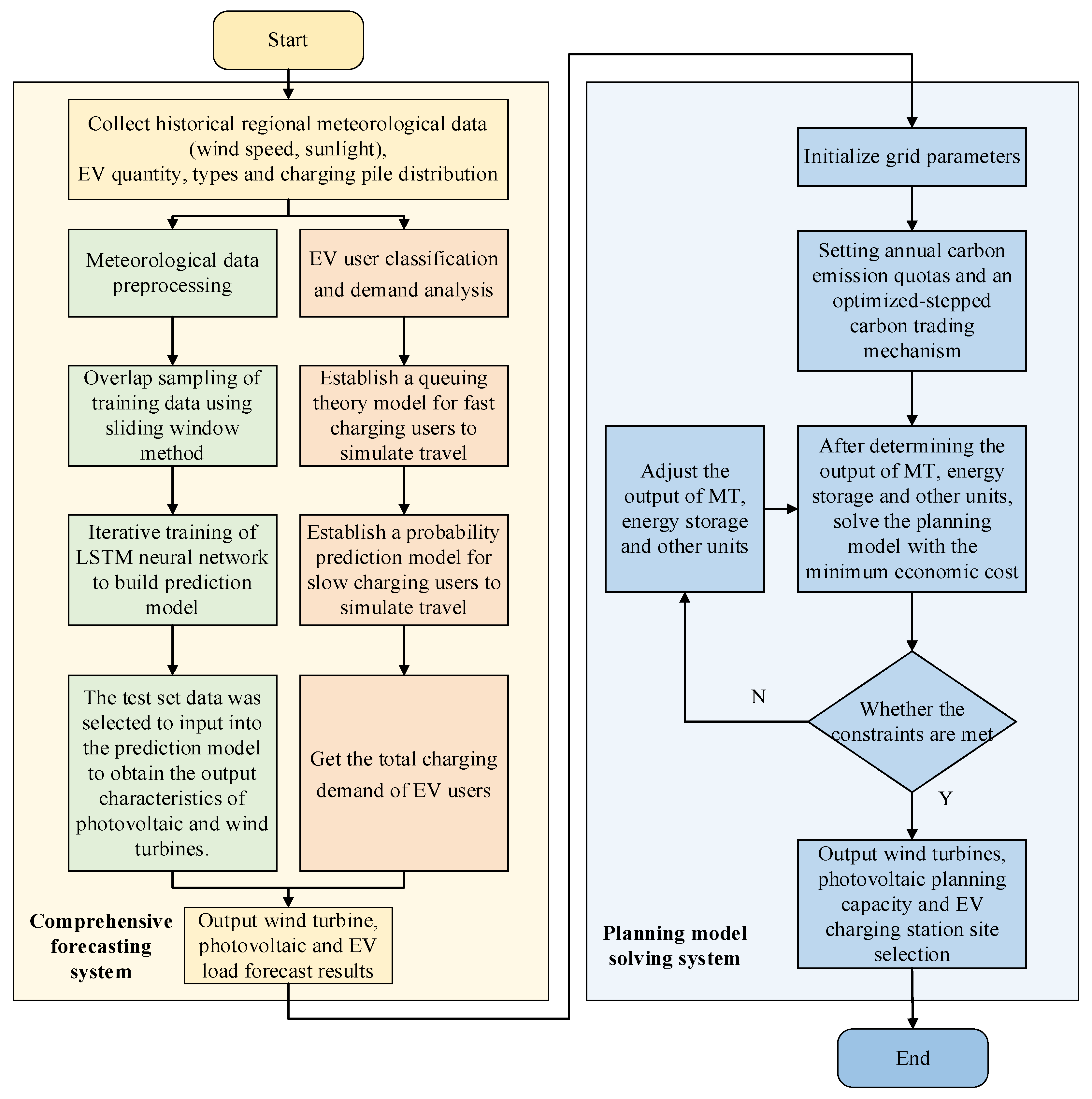
The specific process of implementing the wind power and photovoltaic output model based on CEEMDAN-LSTM is as follows:
First, the data are preprocessed. Historical data are selected to construct a training set and normalized to eliminate the influence of different dimensions.
where
represents the normalized value,
z represents the original value, and
zmin and
zmax represent the minimum and maximum values, respectively.
The original data are decomposed into multiple subsequences and a residual term by using the CEEMDAN algorithm, thereby extracting different characteristic components of the signal.
The processed data are input into the LSTM neural network for iterative training to optimize the model parameters.
The test set data are input into the trained model to obtain the prediction results. The output data are denormalized and restored to the actual physical quantity. The root mean square error (RMSE), mean absolute error (MAE), and symmetric mean absolute percentage error (SMAPE) of the prediction results are calculated to evaluate the prediction accuracy.
The predicted wind speed and light intensity results are introduced into the Weibull distribution model and the photovoltaic Beta distribution model to calculate the output characteristics of wind power and photovoltaic power, respectively [
38].
5. Case Analysis
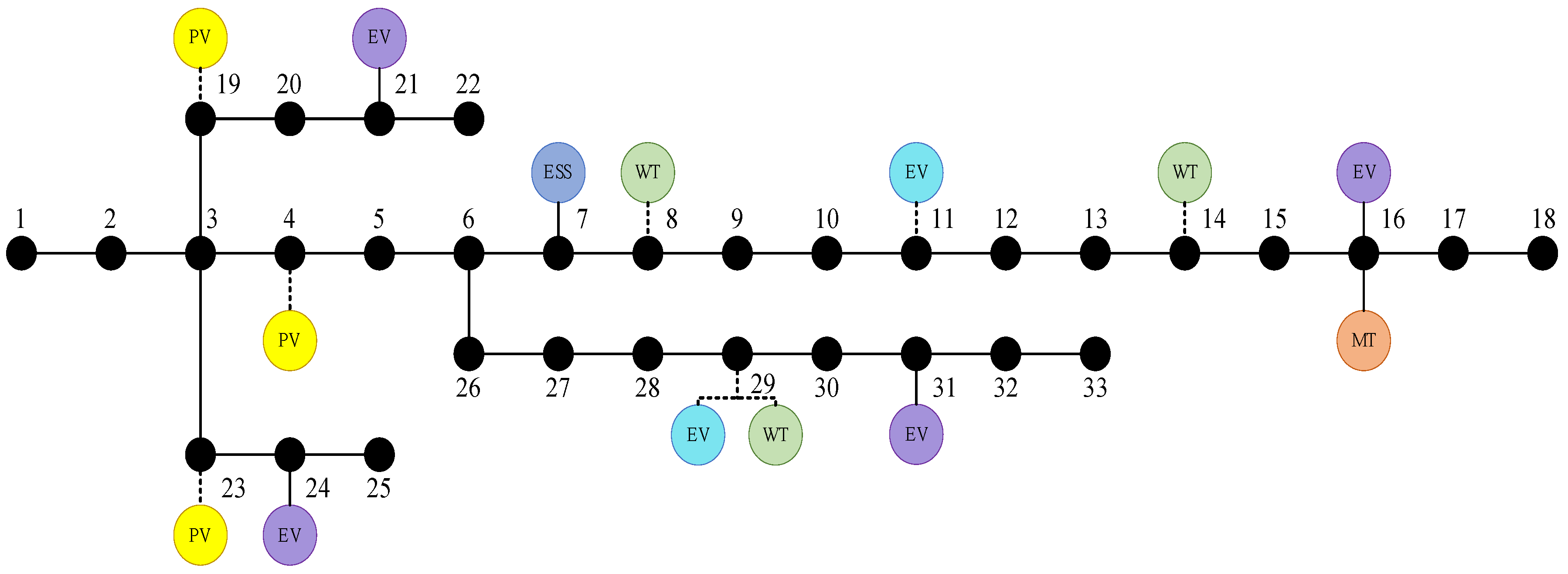
This paper uses the operating data of DG and EVs in a certain region and the improved IEEE 33-node system for case analysis. The case study scenarios are designed to reflect realistic distribution network operations by adopting the IEEE 33-node system—a widely recognized benchmark with radial topology that accurately represents typical grid architectures. The historical wind speed, light intensity, temperature, humidity, and air pressure measurement data of a certain region are used for DG output modeling. The topology of the system is shown in
Figure 4; the dotted lines in the figure represent candidate access nodes for the device, and the solid lines represent the determined site selection nodes for the device. The reference voltage per unit value of each node in the system is 1, and the peak value of the basic active load of the network is 3715 kW. For the EV centralized fast-charging station, four DC fast chargers (3C charging standard) are configured, with a single machine rated power of 175 kW. The optional station sites are nodes 11 and 29. There are 500 electric private cars in the regional EV slow-charging users, all of which use AC slow-charging piles with a rated charging power of 7 kW. The power loss of electric private cars per 100 km is 14 kWh, which is distributed in four large residential areas at nodes 16, 21, 24, and 31. The installed capacity of MT is 500 kW, ESS is a battery energy storage system, the rated parameter is 200 kW/800 kWh, and the charge–discharge energy conversion efficiency is 0.95. MT is connected to node 16, and ESS is connected to node 7. In addition, the optional sites for wind turbines are nodes 8, 14, and 29, and the optional sites for photovoltaics are nodes 4, 19, and 23. The upper limits of the total installed capacity of wind turbines and photovoltaics are 1000 kW and 1500 kW, respectively. The carbon price growth rate
is 0.2, and the carbon price quota interval length
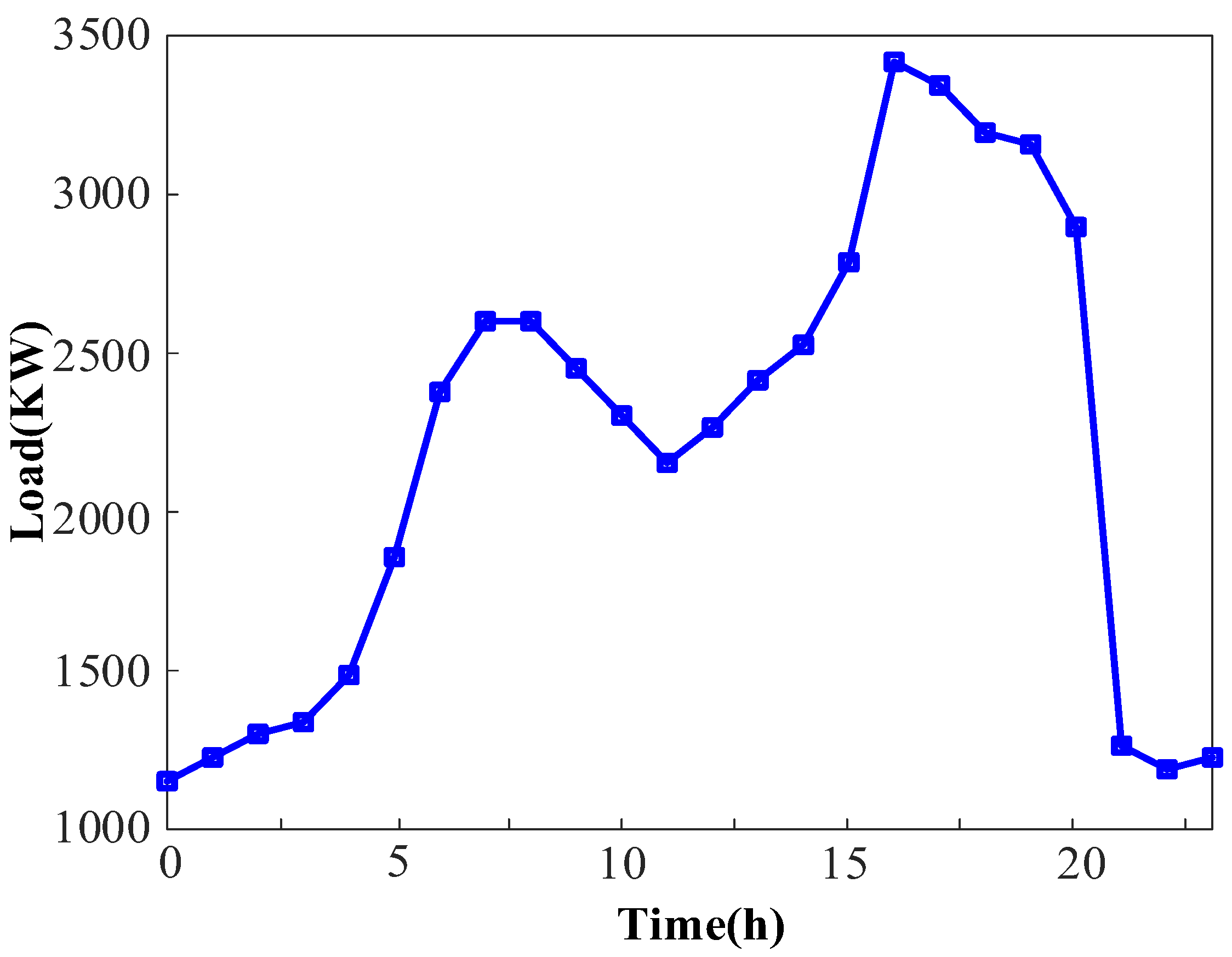
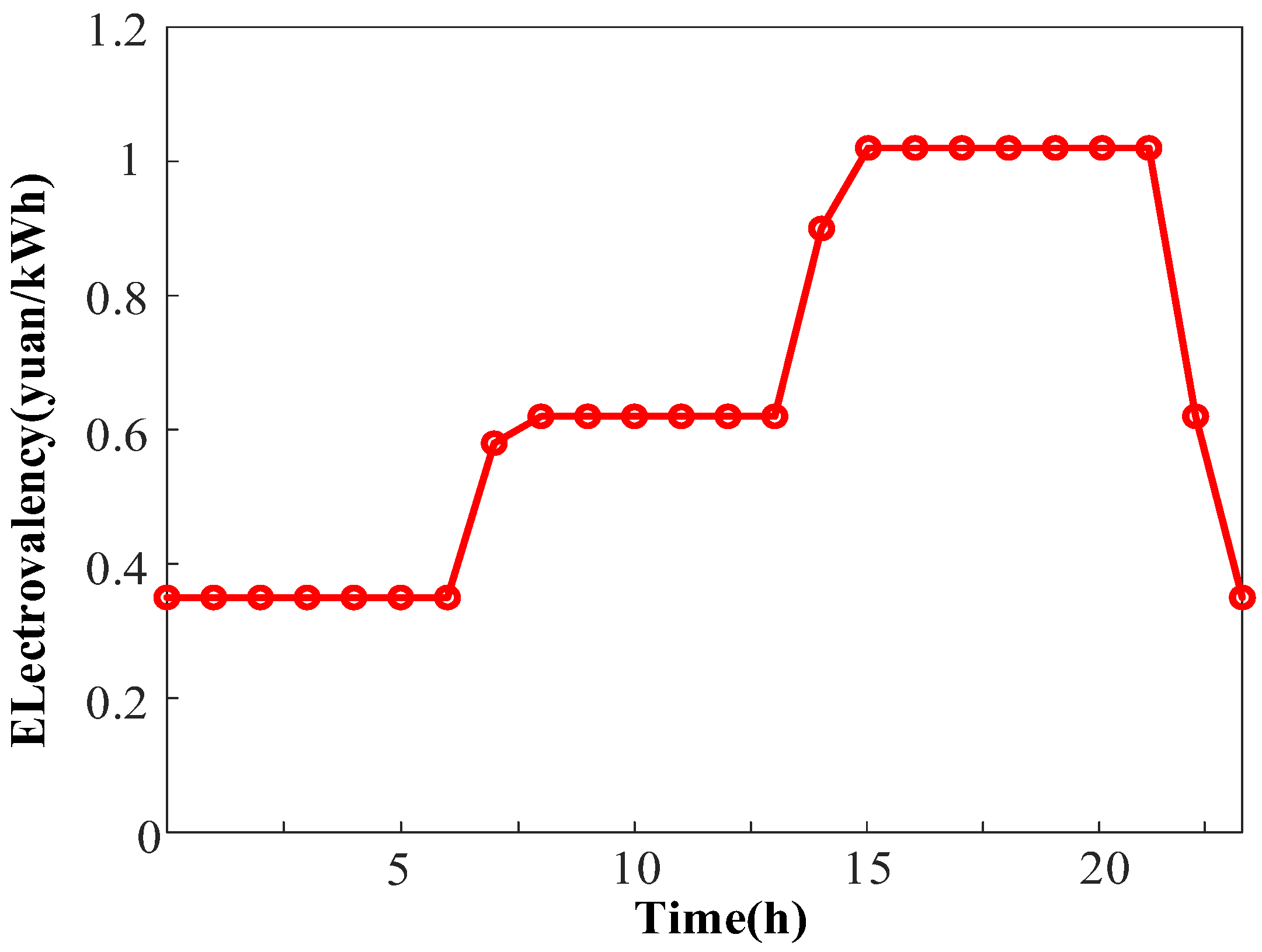
d is 10 t. The typical daily load characteristic curve in the example system is shown in
Figure 5, and the time-of-use electricity price characteristic curve is shown in
Figure 6. Parameters are detailed in
Table 1 [
19].
5.1. Build a Predictive Model
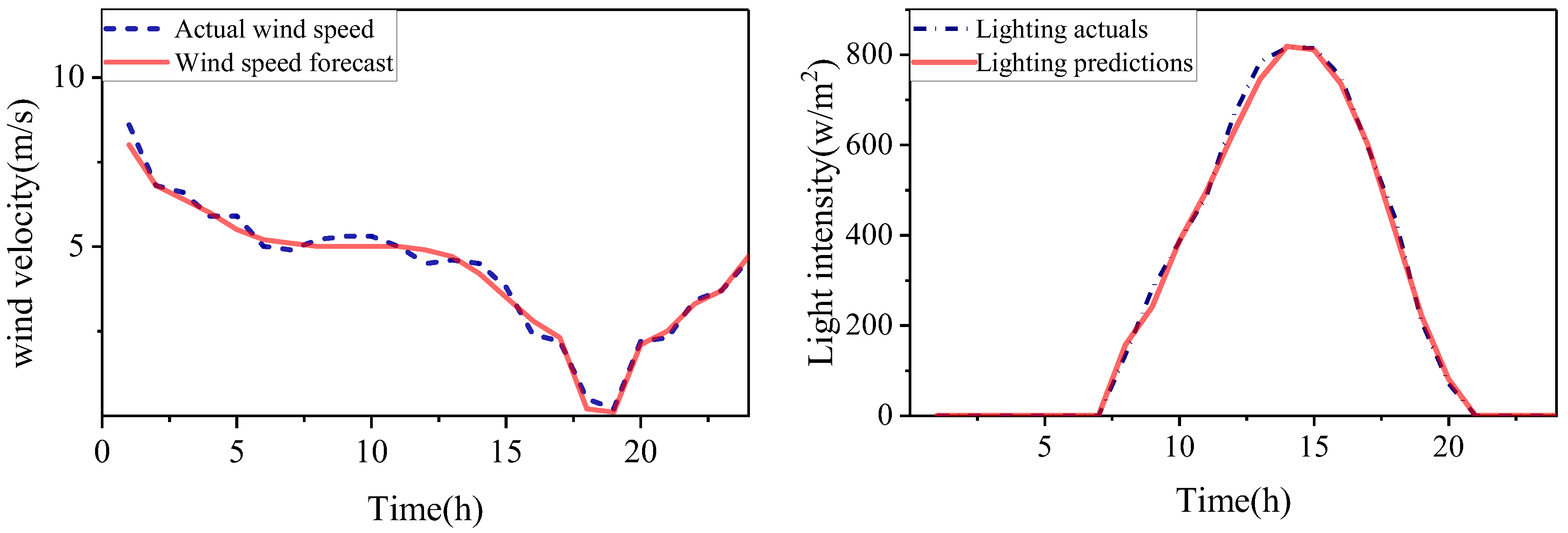
This paper selects relevant historical data of a certain area as the test system. The measurement data interval is 15 min, including historical data of five indicators: wind speed, light intensity, temperature, humidity, and air pressure. The data from August 2019 is used for training and testing. The first 80% of the data in the entire data set is used as the training set, and the last 20% is used as the test set. The prediction results of wind speed and light intensity are shown in
Figure 7.
As illustrated in
Figure 7, the proposed prediction model demonstrates robust performance throughout the 24-h forecasting horizon. Specifically, the model achieves a wind speed prediction accuracy with RMSE of 0.26, MAE of 0.21, and SMAPE of 10.78%. For solar irradiance forecasting, the performance metrics yield RMSE of 16.44, MAE of 9.51, and SMAPE of 3.06%. The LSTM is a basic model and is often used for prediction. The wind speed and solar irradiance are also predicted by the LSTM model. Specifically, the model achieves a wind speed prediction accuracy with RMSE of 0.59, MAE of 0.47, and SMAPE of 19.17%. For solar irradiance forecasting, the performance metrics yield RMSE of 42.18, MAE of 25.24, and SMAPE of 10.63%. Notably, the CEEMDAN-LSTM model exhibits exceptional performance in predicting peak irradiance during noontime periods.
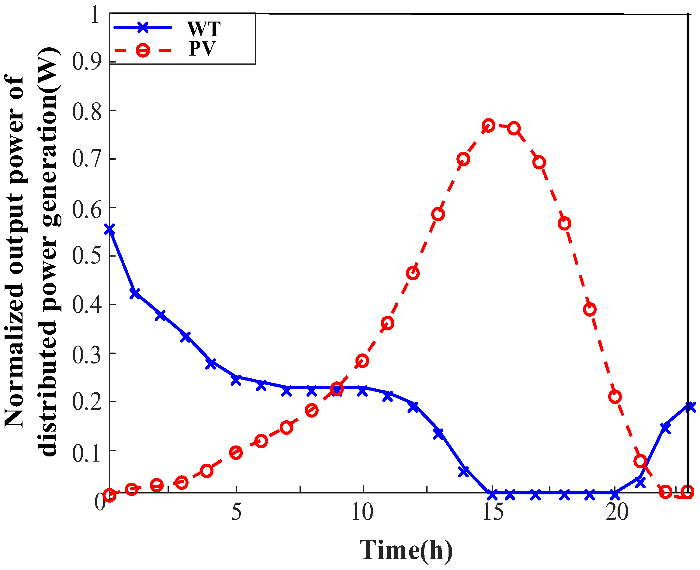
By substituting the wind speed and solar irradiance results obtained from the prediction model into the wind speed Weibull distribution model and the photovoltaic Beta distribution model, the output characteristic curve of DG can be calculated as shown in
Figure 8.
5.2. EV Load Forecasting
Combined with the contents of
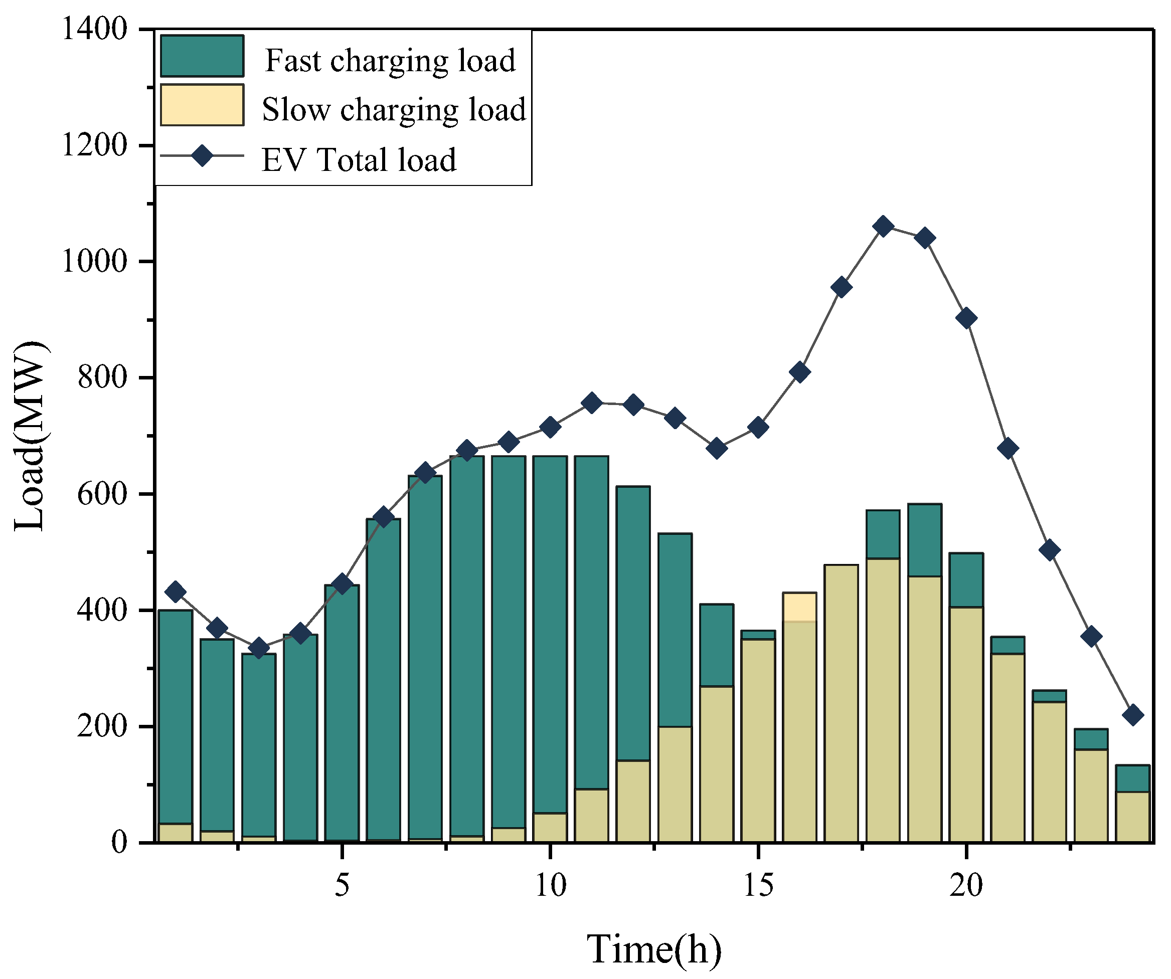
Section 3.1 of this paper, the load demand prediction models for EV fast-charging stations and EV slow-charging users are constructed. Under the corresponding conditions set in the example, the EV load prediction curve is shown in
Figure 9.
The EV load forecasting results reveal distinct characteristics between fast-charging and slow-charging loads. Fast-charging users in this study primarily consist of operational vehicles such as electric taxis and ride-hailing cars, which exhibit significantly different usage patterns compared to private passenger vehicles. Night-shift taxis typically complete their operations and undergo driver shift changes between 8:00 and 10:00. In the proposed model, the taxi shift-change period (te) is incorporated into the Poisson arrival rate ξ, reflecting the reality that many vehicles enter charging stations simultaneously during shift transitions. Unlike private vehicles, operational vehicles must replenish their battery before commencing their workday to ensure sufficient driving range. As a result, the peak in charging demand does not coincide with peak traffic flow. Moreover, the fast-charging load exhibits a pronounced bimodal distribution, with peak demand occurring during 8:00–10:00 and 18:00–20:00, coinciding with commuting rush hours. This pattern reflects fast-charging users’ preference for concentrated charging before and after daily commutes. The slow-charging load curve corresponds to the charging habits of residents during nighttime parking. The combined charging load, formed by superimposing fast and slow-charging demands, reaches its peak during evening rush hours and trough in early morning hours. When further superimposed with conventional residential loads, this combined demand profile significantly elevates grid peak loads, thereby exacerbating the risks of local grid overload.
5.3. Analysis of Planning Results
Combining the planning model established in the previous article and solving it according to the process of 3.3, the planning model solution results are shown in
Table 2.
After introducing the carbon pricing optimization mechanism, the model is solved, and the optimization results are obtained. The wind power installed capacities of nodes 14 and 29 are 107 kW and 893 kW, respectively; the photovoltaic installed capacities of nodes 4, 19, and 23 are 607 kW, 428 kW, and 466 kW, respectively; the EV centralized charging station is configured at node 29; the MT installation node is at 16, with an installed capacity of 500 kW; the ESS installation node is at 7, with an installed capacity of 800 kWh. Thus, some optimization results are obtained. Under this planning, it can meet user needs and minimize the total annual cost. The power purchased by the upper main grid is shown in
Figure 10, the MT output is shown in
Figure 11, and the relationship between the ESS charging and discharging power and the amount of electricity is shown in
Figure 12.
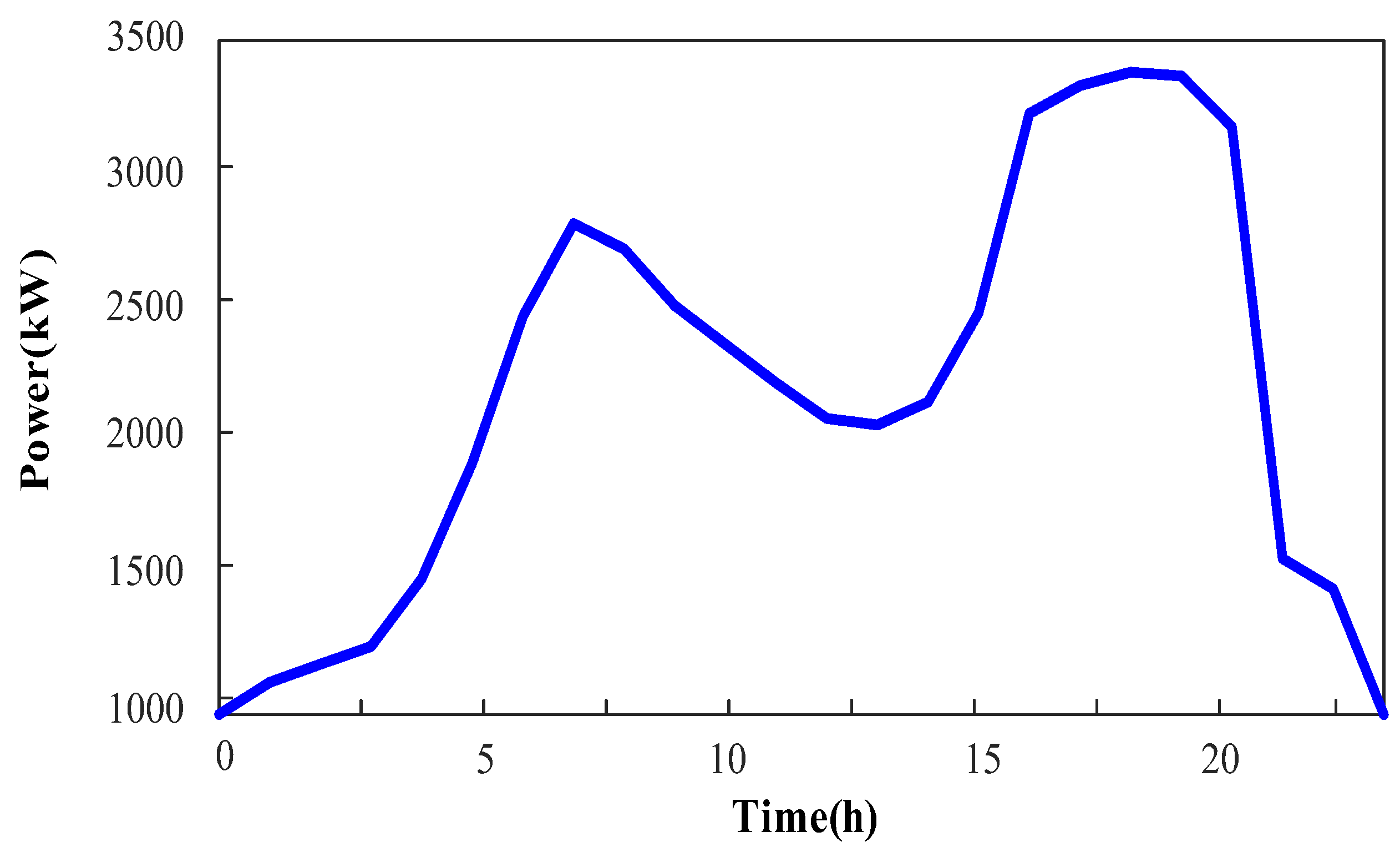
As shown in
Figure 10, the trend of the bulk power purchase curve closely aligns with the load curve. When the load is low, renewable energy sources and gas turbines provide auxiliary power output, resulting in a lower bulk power purchase. During peak load periods, the distribution grid primarily relies on bulk power purchase to meet demand.
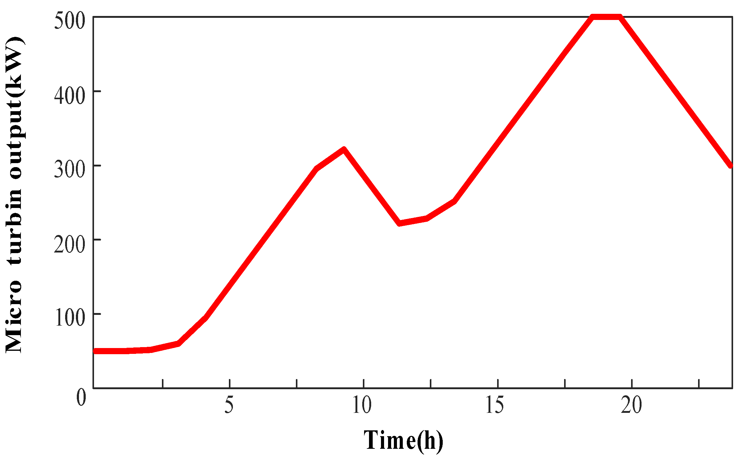
Figure 11 illustrates that the output of the MT is influenced by both the load curve and time-of-use (TOU) electricity pricing. When the load increases or electricity prices are high, the MTs operate at full capacity, reducing bulk power purchase and thereby indirectly lowering electricity procurement costs. From
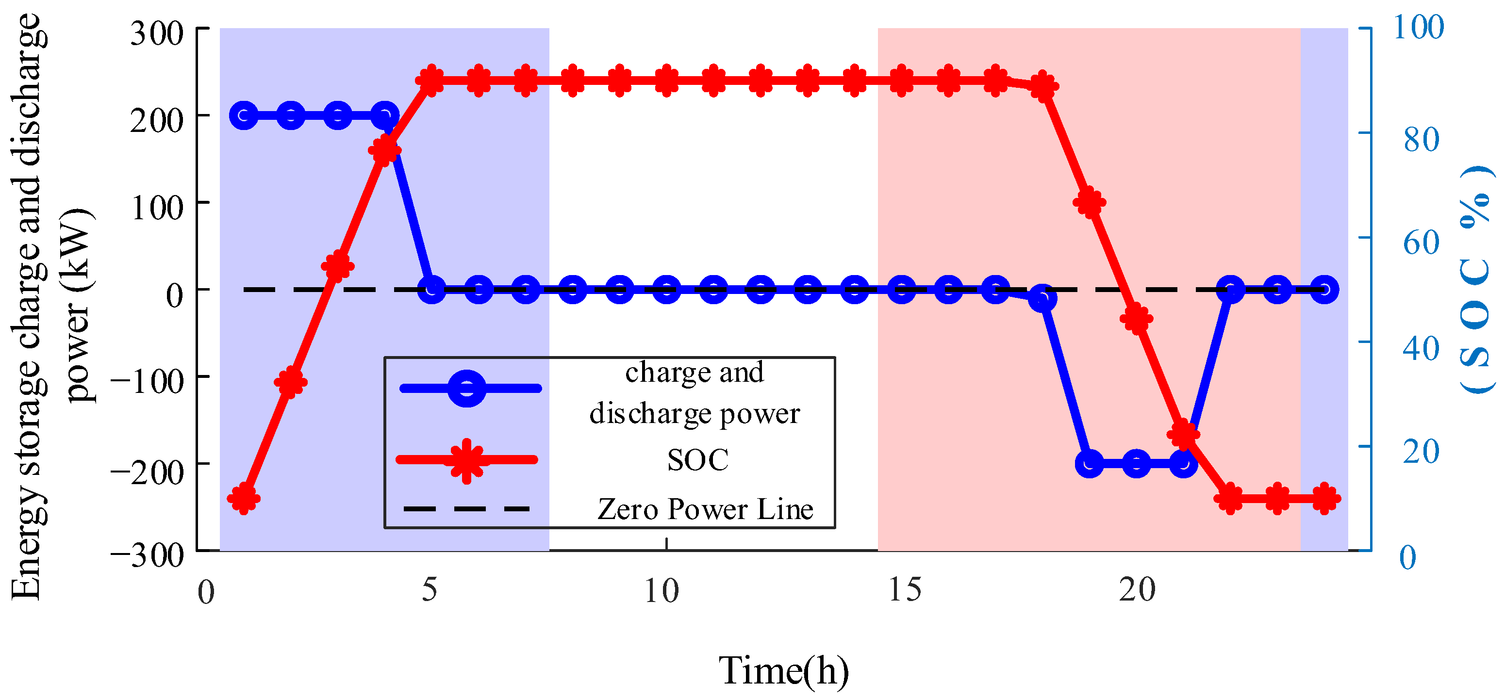
Figure 12, it can be observed that the ESS operates under the dual constraints of TOU pricing and carbon emission costs. The ESS charges when electricity prices are low and discharges during periods of high electricity prices and elevated carbon costs. This strategy reduces bulk power purchase, enabling the distribution grid to indirectly minimize carbon emission costs. The real-time electricity prices and carbon prices guide dynamic ESS charging/discharging, while the dynamic carbon pricing mechanism, in turn, optimizes ESS capacity planning and siting. Through this synergistic mechanism, conventional peak-shaving functions are achieved while creating a new pathway for reducing system emissions by displacing high-carbon grid power. This innovation enables planning solutions to automatically adapt to dynamic changes in electricity and carbon markets, providing new insights for the low-carbon transformation of distribution networks.
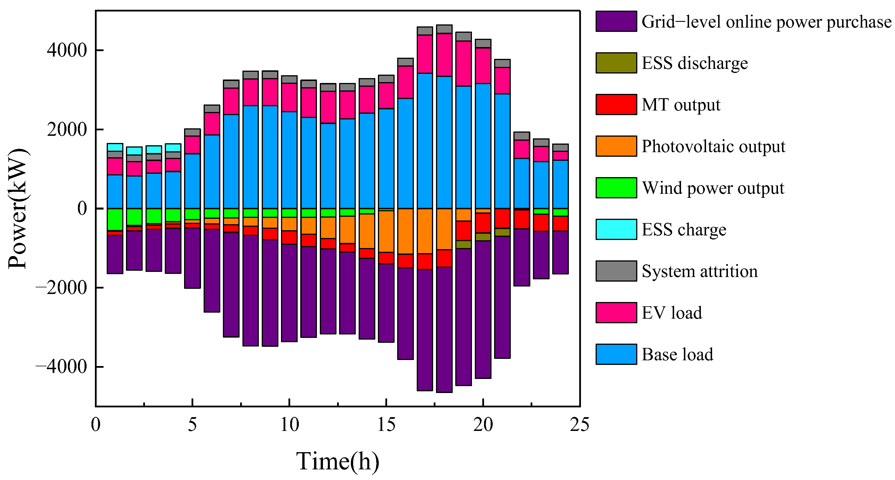
Figure 13 shows the power balance diagram of the distribution grid system. The upper section represents the power demand side, including ESS charging, network losses, and system load demand. The lower section depicts the power supply side, consisting of wind/PV generation, MT output, ESS discharging, and power purchased from the main grid. As evident from the figure, the system maintains power balance over the 24-h period, with total load demand matching total power supply. Renewable generation forecasts guide optimal charging station siting. Dynamic carbon pricing adjusts based on real-time emission levels, creating economic incentives for load-renewable energy coordination. The joint optimization framework iteratively balances these components under technical constraints.
7. Discussion
This study provides a comprehensive framework for the joint planning of renewable energy and electric vehicle charging stations. Although this study establishes a theoretical framework and preliminary validation, in subsequent research, it will be systematically compared with existing planning methods in terms of cost savings, emission reduction, and renewable energy utilization, and a systematic sensitivity analysis will be conducted to evaluate how the uncertainty of carbon pricing schemes and renewable energy forecasts affects planning results. The robustness of this method under extreme conditions of renewable energy and EV loads is discussed, and several important directions for future research are identified. Several important directions for future research have been identified:
Firstly, although our current electric vehicle charging model distinguishes between fast- and slow-charging behaviors, future research will incorporate more refined classifications of electric vehicles, and the impact of climate factors on electric vehicle charging behavior should be considered. To better capture the diversity of charging in the real world. This expansion will provide more tailored infrastructure planning for different user groups.
Secondly, we will expand the evaluation of dynamic carbon pricing mechanisms for different market configurations to assess their adaptability to different policy environments. This analysis will provide practical insights for implementing carbon awareness planning in different regulatory contexts.
Thirdly, there are several technological limitations worth further investigation: (1) the impact of communication delays on real-time carbon price signals, (2) the development of dynamic V2G models that incorporate battery degradation and user incentives, and (3) enhanced prediction techniques for extreme climate events. These improvements will be combined with sensitivity analysis of the system to quantify how uncertainty in carbon pricing and renewable energy forecasting affects planning outcomes.


