Abstract
Given the increasing energy demand and the environmental consequences of fossil fuel consumption, the shift toward sustainable energy sources has become a global priority. Renewable Energy Communities (RECs)—comprising citizens, businesses, and legal entities—are emerging to democratise access to renewable energy. These communities allow members to produce their own energy, sharing or selling any surplus, thus promoting sustainability and generating economic value. However, scaling RECs while ensuring profitability is challenging due to renewable energy intermittency, price volatility, and heterogeneous consumption patterns. To address these issues, this paper presents a Machine Learning as a Service (MLaaS) framework, where each REC microgrid has a customised Reinforcement Learning (RL) agent and electricity price forecasts are included to support decision-making. All the conducted experiments, using the open-source simulator Pymgrid, demonstrate that the proposed agents reduced operational costs by up to 96.41% compared to a robust baseline heuristic. Moreover, this study also introduces two cost-saving features: Peer-to-Peer (P2P) energy trading between communities and internal energy pools, allowing microgrids to draw local energy before using the main grid. Combined with the best-performing agents, these features achieved trading cost reductions of up to 45.58%. Finally, in terms of deployment, the system relies on an MLOps-compliant infrastructure that enables parallel training pipelines and an autoscalable inference service. Overall, this work provides significant contributions to energy management, fostering the development of more sustainable, efficient, and cost-effective solutions.
1. Introduction
As a reaction to climate change, numerous governments and organisations around the world are promoting the shift to renewable energy sources [1], including solar, wind, and hydroelectric power. These sources are naturally replenished on a human timescale and do not exhaust the planet’s finite resources. In this context, communities composed of citizens, businesses, and local authorities—referred to as Renewable Energy Communitys (RECs)—are emerging throughout Europe [2] to make clean energy more accessible and participatory. These communities are designed to promote both self-consumption and collaboration. Members generate their own renewable energy to meet personal demand, and any surplus can be shared locally or sold back to the main grid. These initiatives are not only environmentally sustainable, aligning with the United Nations Sustainable Development Goals [3], but also financially beneficial, as they can significantly reduce electricity costs for participants.
Nonetheless, as these communities expand, managing energy flows and maximising financial returns become increasingly complex tasks. Manual coordination is impractical due to the diverse and evolving energy consumption patterns across households and organisations. Machine Learning (ML) can help streamline these decisions, for instance, by shifting consumption from peak to off-peak hours. However, the unpredictable nature of renewable generation [4], fluctuating energy prices, and changing consumption habits remain challenging, despite the current applicability of static ML models [5]. These are typically trained offline and then used for inference without further tuning, making it difficult to respond effectively to new data distributions. As a result, such methods often yield suboptimal outcomes.
This context demands a new paradigm that enables real-time decision-making, while preserving participant privacy, as energy data can reveal sensitive personal behaviours. In this paper, we present a fully deployed solution based on a multi-tenant Reinforcement Learning (RL) architecture, where each agent independently manages an REC microgrid and aims to minimise operational costs. Recognising that these algorithms cannot be separated from the market environment in which they operate, we enhance the decision-making process through multi-step electricity price forecasting and the introduction of cooperative energy markets. Between communities, we implement a multi-round Peer-to-Peer (P2P) energy trading mechanism, enabling buy and sell bids from RECs to be matched. Within each community, microgrids trade energy via a shared energy pool, either importing from or exporting to the main grid. For both inter- and intra-REC markets, the objective is to maximise the use of available renewable energy and minimise reliance on the Nominated Electricity Market Operator (NEMO)—the authority responsible for market operations in each European Union member state. Finally, as deployment is a core concern of the platform, we integrate key principles from the Machine Learning Operations (MLOps) discipline, including reproducibility, automation, and continuous training and monitoring.
The following sections provide a detailed overview of the solution. In Section 2, we first review the state-of-the-art methods applied in the context of RECs, identifying the main opportunities and challenges in the field. Then, Section 3 focus on the proposed Machine Learning as a Service (MLaaS) system, not only describing the architecture but also the application context in which the solution is meant to operate. This section is followed by Section 4, where we detail the technical components of the system, from the logic and infrastructure levels. In Section 5, we present the experimental setup and the benchmarking results, which testify to the economical viability of our proposal. The source code for both development and evaluation can be found in the following GitHub repository: https://github.com/RafaelGoncalvesUA/rec-simulator (accessed on 2 June 2025). Finally, Section 6 summarises the main contributions of this work and points out aspects to be improved in further research.
2. Background
In this section, we start by acknowledging the role of the 26th UN Climate Change Conference (COP26) in shaping the global energy transition. We then conduct a literature review to gather the state-of-the-art methods applied in the context of RECs, either based on Artificial Intelligence (AI)/ML techniques or complementary to them. The idea is to identify the main challenges and opportunities in the field, as well as gaps in the existing literature. Additionally, we include a performance comparison of predictive models applied in REC contexts, incorporating several studies that, while not part of the formal literature review, are still relevant to the domain of energy forecasting—a critical component in REC decision-making.
2.1. Role of COP26 in Energy Transition
A pivotal moment in the global energy transition was the 26th UN Climate Change Conference (COP26), which reinforced the urgent need for countries to commit to decarbonisation, adopt cleaner technologies, and decentralise energy systems. In line with these objectives, recent studies have explored innovative and location-specific solar energy solutions that support sustainable development and climate resilience. For example, a novel solar still design tested in Yekaterinburg, Russia, demonstrated a low-cost method of freshwater production by enhancing the evaporation–condensation process, using solar thermal energy [6]. Such technologies are crucial for addressing water scarcity in off-grid or rural areas, while minimising reliance on fossil fuels. Currently, there are also techno-economic studies in the literature that evaluate the feasibility of the integration of these kinds of sources. One study [7] examined the use of solar tracking systems in South India to improve electricity generation from solar panels, showing how such innovations can make renewable energy more accessible and viable in regions with high solar potential. These studies exemplify how tailored renewable energy solutions are advancing the global climate agenda set by COP26. The next subsection provides an in-depth analysis of multiple studies conducted in REC settings, which have thus contributed to expanding access to renewable energy, improving efficiency and promoting low-carbon development.
2.2. Existing REC Solutions
In [8], the authors present an intelligent framework to manage energy demand and Photovoltaic (PV) generation, aiming to maximise REC profitability. Their hybrid method combines a Time Delay Neural Network (TDNN) with a stochastic Model Predictive Control (MPC) approach. The TDNN forecasts several steps ahead using time delays and a sliding input window, capturing long-term dependencies more effectively than standard neural networks and training faster than methods like Long Short-Term Memory (LSTM). The MPC then uses these predictions to optimise costs by solving a profit-maximising problem at each step while respecting operational constraints. The Battery Energy Storage System (BESS) plays a key role in handling forecasting errors by reserving capacity to balance surpluses and shortages, improving both economic and grid performance. However, the method has not been validated across multiple RECs. Future work may include weather data integration into the TDNN. Regression techniques are also used to monitor electrical transformers, helping RECs manage congestion in low-voltage grids. In [9], Mai et al. train models using voltage magnitude data from a small number of Smart Meters (SMs) at the Point of Connection (POC), preserving user privacy while still reflecting grid status. However, the study does not account for changes in grid structure or new PV additions. Regular model updates are recommended for deployment.
To address both user privacy and system scalability, Federated Learning (FL) is being employed in energy management contexts [10], where agents such as Virtual Power Plants (VPPs) or central community operators are involved. Using a Consensus + Innovations’ approach, agents forecast net demand and agree on a common strategy (Consensus), while still optimising local resources independently (Innovations). Although the system manages the limitations caused by decentralised optimisation, the challenges related to non-stationary data distributions remain unaddressed.
Accurate energy forecasting is essential for REC efficiency. In [11], a decision-making algorithm is proposed to guide trading actions—buying, selling, or storing energy—using XGBoost combined with forecasting modules for PV output, battery SoC, and market prices. These forecasts inform battery operation to reduce energy costs. The paper notes XGBoost’s parallelisation advantages, but would benefit from deeper hyperparameter tuning.
One potential issue in this context is the lack of high-resolution energy data. In [12], this is addressed using a non-intrusive method that reconstructs load profiles from monthly billing data with a combination of unsupervised and supervised learning. Users are first clustered by behaviour (e.g., via K-means), then typical patterns are assigned with a classifier. These profiles are normalised and scaled using monthly consumption. Despite the realistic profiles that the method yields, this study does not address the correlation between the reconstruction error and relevant REC features, such as the number and type (residential, commercial, etc.) of habitants.
Another study in the field [13] focuses on battery scheduling for both short-term operations and long-term planning, introducing a bi-level Reinforcement Learning (RL) framework. The short-term model reduces peaks and boosts profits, while the long-term model handles investment and lifecycle strategies. It considers dynamic factors like battery prices and electricity rates. Although no retraining is included, we highlight that the model adjusts to gradual data changes over time, especially price fluctuations.
In opposition to common centralised management systems, Peer-to-Peer (P2P) trading allows direct exchanges between community members. In [14], R. Densyiuk et al. propose a market mechanism that promotes self-consumption before trading, discouraging overproduction and excess demand. The system uses dynamic pricing, based on game theory, and penalties to guide behaviour and maintain local energy balance. While conceptually innovative, the paper lacks implementation details.
Despite AI advances, traditional analytical tools remain valuable. Game theory methods—e.g., the nucleolus, Shapley value, and Shapley-core—help fairly divide costs and benefits in RECs. Ref. [15] demonstrates that no method ensures full fairness and stability simultaneously. Results suggest that the Shapley value suits small communities, while nucleolus and Shapley-core perform better in larger ones, although all have high computational demands. A scalable implementation is not provided, but RL-based approximations are suggested as a future direction. In [16], a framework is proposed for sharing collective PV and battery storage within RECs, comparing different energy justice approaches. Each method redistributes benefits based on participation, aiming for fairness and equity. Results show that shared storage improves fairness, especially under dynamic models. The study highlights the role of energy justice and game theory in designing equitable asset-sharing mechanisms.
Regarding RL techniques, a recent study [17] presents a multienergy regional energy market model that employs a price-matching mechanism and hierarchical RL (HRL) to perform day-trading decisions. Unlike traditional setups, this model facilitates cross-energy-type transactions (electricity, gas, heat), while preserving user privacy and autonomy. A joint trading mechanism accounts for the varying transmission speeds and time scales of different energy types. The proposed HRL approach divides policies into subpolicies of different levels and thereby addresses the large state–action space and sparse rewards by decomposing decision layers, improving convergence and reward stability. Simulation results show improved matching success and operator rewards. This work advances both market design and learning algorithm application in multi-energy trading environments.
Unlike other papers focused on specific techniques, E. Karakolis et al. [18] introduce I-nergy—a broader initiative for an AI-on-demand platform tailored to energy communities. The proposed architecture includes layers for data services, pre-trained models, analytics, and links to the AI4EU infrastructure. It envisions a suite of AI services, including forecasting, optimisation, and trading. While pilot cases are listed, the focus remains on conceptual design rather than on concrete implementation.
Although all these studies contribute valuable insights, most fall short of meeting key requirements for a full MLaaS solution. Table 1 summarises the main features in the existing literature and contrasts them with what is needed to answer the proposed research questions. Conceptual works without technical implementations were excluded as complete solutions.

Table 1.
Related work comparison (✓ denotes ‘present’, X denotes ‘absent’).
The analysis reveals that some of the studies focus primarily on developing specific AI models for tasks such as energy forecasting, user consumption profiling, and battery management. Others explore technical aspects of ethical concerns, including fairness and data privacy. One paper introduces the AI on-demand paradigm as a step towards deploying models in a cloud environment; however, it lacks a comprehensive implementation strategy. With regard to model deployment and lifecycle management, the reviewed studies generally do not present clear or robust procedures. Furthermore, inconsistencies in the performance metrics reported across studies hinder meaningful comparisons of model effectiveness. Although metrics such as Mean Absolute Error (MAE), Root Mean Squared Error (RMSE) and Mean Absolute Percentage Error (MAPE) are presented, none of the studies discussed approaches for tackle model degradation in real-world deployments.
2.3. Predictive Models in REC Settings
Beyond the literature review, it is essential—as in any ML task—to benchmark state-of-the-art models as performance baselines and to enable informed hyperparameter tuning. To this end, we compiled top-performing models from various REC studies, focusing on their performance metrics: MAE, RMSE, MAPE, or Relative Mean Absolute Error (rMAE)—a normalised version of MAE. While some of these papers were excluded during earlier phases of the systematic review, they remain relevant due to their practical energy forecasting contributions. For this comparison, we restricted our focus on predictive tasks (e.g., demand, PV output, electricity price), intentionally excluding broader energy management frameworks that cannot be directly compared to regression models and are typically assessed using different economic KPIs in REC contexts. Additionally, studies that did not clearly identify the best model or failed to average results across multiple experimental runs were left out of the comparison.
Aside from model performance, Table 2 also captures other relevant factors, such as the unit of the target variable (e.g., kW, kWh), the temporal granularity of predictions (e.g., 15 min, hourly), model type (univariate or multivariate), and the structure of input/output windows (e.g., past 5 h to forecast next 30 min), which are all critical to evaluating the suitability of a model for a specific application.
Table 2.
Overview of common prediction tasks in RECs.
Table 2 underlines the challenge of comparing different models due to the lack of consistency in evaluation metrics across the studies. Even when identical metrics are reported, the results often represent averages over varying numbers of trials, making standard deviation an important factor in assessing model robustness. Moreover, many studies omit statistical significance testing, which would help determine whether observed performance differences are meaningful or merely the result of random variation. Differences in experimental setups—including the number of buildings analysed and the input/output time window sizes—also introduce variability that complicates direct comparison. To improve the fairness and utility of future comparisons, studies should apply a broader range of evaluation metrics and attempt to replicate—or closely approximate—the experimental conditions of prior research.
3. Methodology
3.1. Application Context
For efficient energy management and trading, the MLaaS system should be grounded in the real-world energy ecosystem it is meant to support: a large network of prosumers, consumers, and batteries from different households or local organisations. All of them would be connected to a Virtual Power Plant (VPP) that manages the energy trading between the REC grid and the energy market, which is Operador do Mercado Ibérico de Energia (OMIE) in our application context, thereby deciding whether to buy, sell, or resort to the batteries. As illustrated in Figure 1, the VPP is the central entity that executes the final trading decisions, and its role is to aggregate the energy demand and supply of the communities, and to communicate with the energy market.

Figure 1.
Application context of the proposed solution.
As each REC is composed by multiple microgrids with heterogeneous energy demands and generation patterns, a multi-tenant cooperative solution is needed to manage the energy flows. For instance, the energy demand of a small household is not the same as that of a corporate building. As further discussed in the next section, the habits and preferences of all tenants must be taken into account, which imply different trading strategies, but only one final decision per community can be taken by the VPP.
3.2. Proposed MLaaS Solution
Framing the application context in line with the MLaaS paradigm, each microgrid can be referred to as a tenant. Each tenant is managed by an intelligent agent, and a set of these tenants forms an REC, which ultimately negotiates collectively with other RECs and the Nominated Electricity Market Operator (NEMO). The architecture shown in Figure 2 illustrates how the proposed MLaaS setup can be operationalised, detailing the software stack and the interactions between its core components.

Figure 2.
Overview of the implemented system architecture.
We assume an REC j consisting of N microgrids, each paired with its own agent, but sharing a unified energy pool. At regular intervals, the simulated microgrids (i.e., tenants) emit observations, much as real IoT devices would. These observations are then routed to two key modules: a relational database and an inference service. The database is a TimescaleDB instance that stores these microgrid readings—denoted obs1, …, obsX, where X represents the maximum number of observations per microgrid, and uses a schema indexed by tenant ID and timestamp. The inference service is implemented with KServe, which exposes a custom prediction endpoint to handle incoming observations in real time and output control actions for the microgrid.
Simultaneously, a Python-based data collector polls the database at intervals, gathering recent data points for specific tenant IDs. This data is buffered, and when certain predefined conditions are met (such as elapsed time or buffer size), a Kubeflow pipeline is triggered. This pipeline utilises pre-built Docker containers containing all necessary dependencies, and either trains a new agent or fine-tunes an existing one. Once training is complete, the updated agent is saved to a MinIO object storage system and deployed via the inference service, which is alerted of the model update. The corresponding microgrid records in TimescaleDB are then removed.
The architecture supports dynamic scaling of both the inference services and databases, uses a single instance for the data collection process, and runs up to N concurrent Kubeflow pipelines, where N is the number of microgrids being managed. All components are deployed within a lightweight K3s Kubernetes cluster.
The system is also privacy-preserving. Each intelligent agent only has access to their own microgrid/ tenant data, and no data are shared between agents. Their reward function is designed to optimise the performance of each microgrid independently, without requiring access to data from other microgrids. Nevertheless, as detailed in Section 4.4 and Section 4.5, through intra and inter-REC energy exchanges, communities and consequently microgrids can indirectly benefit from their peers’ optimal decision-making, since a common energy pool is used for trading in the market.
Regarding the software stack, our MLaaS framework integrates several carefully selected tools and libraries designed to provide a balance between performance, scalability, and edge compatibility. At the infrastructure layer, K3s—a lightweight Kubernetes variant—is employed for service orchestration. Docker is used to containerise ML training environments and frameworks, ensuring consistency, portability, and ease of deployment within Kubernetes. For serving models, KServe is used to expose autoscaling REST endpoints, with Knative support enabling scale-to-zero capabilities. Kubeflow manages the ML pipelines, providing reproducible training workflows with deep Kubernetes integration and support for custom pipeline components. Trained agent models are stored using MinIO, an S3-compatible, Kubernetes-optimised object storage service. Time-series data, generated by the microgrids, is handled by TimescaleDB, a PostgreSQL-based database that supports complex SQL queries and scales well with time-dependent data. For simulation, we use Pymgrid, which offers a flexible and realistic environment for modelling microgrid behaviour and supports integration with RL frameworks. Lastly, agent training is handled by stable-baselines3, a PyTorch-based library offering state-of-the-art RL algorithms tailored for control and energy management tasks.
3.3. RL Formulation
To apply and evaluate RL algorithms, we used and extended the discrete environment provided by the Pymgrid library, CsDaMicroGridEnv. This environment wraps around a microgrid instance and is compatible with the OpenAI Gym interface, widely used in RL research. At each simulation step, the execution flow involves gathering observations from the microgrid, normalising them, converting the selected discrete action into a prioritised list of continuous control operations (see Section 3.3), executing the corresponding action, and computing the resulting reward.
The environment initially includes an 11-element state vector composed of energy load, PV generation, battery state of charge [0.0–1.0], battery charging and discharging capacity [0.0–1.0], grid availability, CO2 emissions from the grid, import/export energy prices, and the current hour represented through two cyclical features: and (as shown in Equation (1)). Using cyclical encoding instead of raw hour values allows the model to learn time-related patterns, such as the proximity of 23:00 to 00:00.
The state vector, S, is extended by integrating price forecasts to improve the agent’s decision-making. Including all forecast steps from a multi-step predictor would excessively inflate the vector dimensionality, increasing model complexity and training time. To address this, we select three representative forecast values for a prediction horizon f: the first step (), one intermediate step (), and the final step (). This method provides a summary of the forecast trend while maintaining a manageable state size of 14 elements, as shown in Equation (2). Further discussion on forecasting methods is presented in Section 4.1.
- : base state vector element at index i (e.g. energy load, PV generation, etc.);
- , : cyclical features for the current hour;
- , , : forecasted energy prices at different steps (initial, intermediate, and final).
Regarding the action space, the environment defines 7 discrete actions, encoded as integers. Each action corresponds to one or more operational commands, which are executed depending on the availability of energy resources. Table 3 details the available actions, their respective operations, and the primary components involved, excluding the renewable sources (PV) and consumption modules.
Table 3.
Actions and corresponding operations (✓ denotes ‘present’, X denotes ‘absent’).
Actions 0, 3, and 5 are primarily designed to manage surplus energy through either the battery or the grid. In contrast, actions 1, 2, and 4 focus on fulfilling current energy demands using the battery, grid, or genset (if available). These actions act as priority commands, and both energy supply and surplus handling can occur simultaneously if mapped accordingly.
To guide the agent’s learning, we define the reward function as the negative total operational cost. As expressed in Equation (3), at timestep t, the total cost () includes grid import costs along with potential penalties from unmet demand, surplus energy, battery usage, and fuel consumption (genset), minus any revenue from energy exports to the REC’s grid.
- : Energy imported from the grid (kWh);
- : Energy exported to the grid (kWh);
- : Cost of trading 1kWh of energy with the grid (same value for importation/exportation, in this case);
- : Cost of operation i (loss load, overgeneration, battery use and genset).
For separate training and testing contexts, the simulator allows data splitting by percentage. We used the default configuration: 67% for training (5870 hourly steps, about 244.58 days) and 33% for testing (2890 steps, about 120.42 days). Although longer training could enhance learning, a broader test window helps capture seasonal variation, leading to more robust evaluations. With this setup, all algorithms were trained over 100,000 steps, roughly equivalent to 17 episodes.
3.4. Available Energy Profiles
The simulator offers a collection of microgrids featuring realistic and diverse load and PV generation profiles drawn from various climate zones across the United States. These time series contain 8760 hourly data points, representing an entire year.
By performing a detailed Exploratory Data Analysis (EDA) on these datasets, key patterns and trends can be uncovered and utilised by RL algorithms. Specifically, using seasonal decomposition, the time series can be broken down into trend, seasonal, and residual components. This helps reveal the long-term behaviour of the data, recurring seasonal patterns (such as daily or weekly cycles), and any anomalies or noise. For instance, selecting a random microgrid, we observe that the average daily load increases during the first half of the year (see Figure 3), peaking in summer—likely due to air conditioning use—and then gradually decreases in the latter half. The seasonal component reveals a consistent weekly cycle, with higher demand on weekdays and lower demand on weekends. The residuals are mostly centred around zero, indicating that the decomposition captures most of the data’s variability. Similarly, the PV generation shows a seasonal trend, peaking during the summer months when solar radiation is strongest.

Figure 3.
Seasonal decomposition of the energy load profile of an arbitrary microgrid (no. 3 in Pymgrid25 dataset).
4. Development
4.1. Energy Price Forecasting
To improve the decision-making capabilities of the intelligent agents, we incorporated a forecasting module that predicts future energy prices over time. This component is essential for allowing agents to make more strategic choices regarding energy usage, such as when to charge or discharge batteries, when to import or export energy, or when to activate backup generators. By having access to reliable forecasts of upcoming energy prices, agents can adapt their actions to reduce costs and increase savings. For this reason, rather than using synthetic energy price data, we opted for real-world data from OMIE. This allowed us to not only evaluate forecasting accuracy but also integrate the real prices directly into the microgrid’s reward calculation. Using the open-source library ‘OMIEData’ https://github.com/acruzgarcia/OMIEData, (accessed on 2 June 2025), we collected hourly historical data for the entire year—from 1 January to 31 December 2024. From this dataset, we extracted Portugal’s marginal energy price, which reflects the cost of producing one additional Megawatt-hour (MWh) of electricity to satisfy demand.
Before model training, we performed an EDA (exploratory data analysis) of the energy price series. Our initial step consisted of visualising the distribution (see Figure 4). The results revealed a maximum price exceeding 190 MWh, along with multiple modes (peaks) suggesting the presence of different market dynamics, such as peak and off-peak conditions. The highest density occurs in the lower price range, between 0 and 10 EUR/kWh, likely driven by times of abundant renewable energy or low consumption (e.g., nights or weekends). In contrast, the long right tail indicates occasional price surges, typically caused by spikes in demand or supply disruptions. The intermediate peaks may correspond to transition periods when the energy mix is shifting.

Figure 4.
Electricity marginal price KDE (red region = interquartile range).
In previous research [24], forecasting models like ARIMA (AutoRegressive Integrated Moving Average) and GRU (Gated Recurrent Unit) delivered strong results and proved effective for localised home automation applications due to their short training times. However, we also observed that NeuralProphet offers greater usability, adaptability, and interpretability, making it a promising candidate for larger-scale implementations. It additionally addresses a key limitation of ARIMA: its requirement for regularly spaced data and manual handling of missing values.
NeuralProphet builds upon Facebook’s Prophet model by incorporating Artificial Neural Networks (ANNs), enabling it to model more complex temporal dependencies while preserving its explainability. Similar to Prophet, it decomposes time series data into trend, seasonality, and special events, but allows these components to be customised flexibly. Unlike Prophet, it includes autoregressive terms through a feed-forward neural network to better capture short-term dynamics. Its modular structure facilitates customization, making it ideal for tasks that need both model interpretability and expressive power. In terms of preprocessing, it automates tasks like datetime parsing, frequency detection, handling gaps in timestamps, and normalising features. It models seasonal patterns using Fourier series with auto-selected terms and supports lagged as well as external regressors, internally aligned and encoded. Additionally, it automatically identifies and scales trend change points and performs training–validation splitting based on the forecasting horizon.
Choosing the appropriate lookback and forecast windows is essential in any forecasting setup, as highlighted in previous work [25]. The lookback window must be long enough to include meaningful trends, but short enough to avoid unnecessary noise, while the forecast horizon should reflect the planning requirements of the agents. Increasing the number of forecast outputs raises the state space dimensionality, which can lead to overfitting and higher computational demands. Therefore, a careful balance is required to ensure that agents receive sufficient input without overwhelming the model. While dimensionality reduction methods can help, as discussed in the previous study, they often come at the cost of reduced explainability. As an alternative, we chose to retain only a subset of steps from the forecast horizon.
During training, we configured the model to run for 50 epochs with a batch size of 32. We experimented with different combinations of lookback and forecast windows, as described in Section 5, to determine the most effective setup for our scenario. Due to significant seasonal fluctuations in energy pricing, we divided the dataset into 10 folds and implemented a time-based cross-validation approach. This method preserves temporal order, preventing leakage of future data into the training set. As in standard cross-validation, performance was averaged across folds to determine the final result. Since there were no signs of overfitting, we did not apply any regularisation techniques.
4.2. Intelligent Agents
The system’s logic is driven by intelligent agents, whose decisions shape not only individual microgrid behaviour but also the community’s overall energy trading strategy. Efficient microgrids reduce reliance on grid imports, while poor internal decisions can lead to increased external energy dependency. The agents are therefore designed to optimise a reward function defined as the negative of the energy cost. At every time step, the agent receives an observation vector, selects the next action, receives a corresponding reward, and updates the neural networks that represent its policy. For this study, we implemented and evaluated three widely used RL algorithms from the stable-baselines3 library [26]: Deep Q-Learning (DQN), Proximal Policy Optimisation (PPO), and Advanced Actor–Critic (A2C). Their performance was benchmarked against a fixed-rule baseline agent.
Due to the large number of variables and the diversity of microgrid scenarios, we chose to fine-tune three key hyperparameters: the activation function, the learning rate, and the number of hidden units per layer in both the policy and value networks. Existent work [27] indicates that DQN and PPO are less sensitive to changes in learning rate compared to A2C, and it highlights the value of experimenting with network architecture, underlining the relevance of these parameters. The paper also stresses that using a high discount factor, , helps to prioritise long-term rewards over short-term gains—an important aspect in energy optimisation tasks.
Alongside automated tuning and cross-scenario testing, we tailored the hyperparameters individually for each algorithm. Each subsection outlines the most relevant settings used. Some choices were influenced by computational limitations—for example, setting the number of PPO epochs to 10 to strike a balance between training efficiency and model performance. Other parameters required manual tuning within selected test environments—for instance, carefully adjusting DQN’s exploration rate to reduce excessive randomness. A complete evaluation, with fixed parameters and variations in learning rate, network configuration, and test setup, is provided in Section 5.
4.2.1. Heuristics-Based Agent (Baseline)
Evaluating an agent solely based on its cumulative cost does not provide a complete picture of its performance. The agent may be executing a suboptimal policy, or the environment itself might be incompatible with the chosen strategy. To better assess the effectiveness of the implemented RL algorithms, we compare them against a heuristics-based agent used as a baseline. This agent follows a basic rule-based logic designed to imitate the decision-making of a human operator based on the observation vector. By defining the net load of the microgrid as the difference between the demand and the energy generated by the PV panels, the agent operates according to the rules outlined in Figure 5.

Figure 5.
Decision tree of the heuristics-based agent.
In essence, the agent first determines whether or not the PV panels are generating surplus energy. If excess energy is available, it attempts to charge the battery—provided that the battery is not already full or degraded. If the battery cannot be used, the agent exports the surplus to the grid. Conversely, when PV generation is insufficient to meet the load, the agent tries to discharge the battery, unless it is depleted or degraded. If battery discharge is not an option, the agent imports the shortfall from the grid. In the case of a zero net load—when production exactly matches consumption—the default action is to import energy from the grid, though the actual result within the microgrid is effectively idling.
4.2.2. Algorithm 1: Deep Q-Learning (DQN)
Deep Q-Learning (DQN) is a value-based RL approach designed specifically for discrete action spaces [28]. It extends the classic Q-learning algorithm, which estimates the action–value function, , for each state–action pair. Both algorithms aim to learn a mapping from pairs to their expected cumulative rewards. The resulting policy is derived by selecting the action that maximises the predicted Q-value. The key distinction is that DQN leverages a deep neural network to approximate the Q-function, allowing it to scale to high-dimensional observation spaces. DQN also incorporates two major improvements over traditional Q-learning: experience replay and a target network.
Experience replay maintains a buffer of past interactions (state, action, reward, next state), from which it samples mini-batches during training. This process reduces temporal correlations in the data and lowers update variance, leading to more stable learning dynamics.
The target network is a separate copy of the Q-network used to compute the target Q-values during training. It is updated less frequently and provides a fixed reference for a number of steps, improving stability. Updates are based on an approximated Bellman equation (see Equation (4)), which adjusts Q-values towards the sum of the immediate reward and the discounted maximum future reward. The discount factor controls the trade-off between immediate and future gains. This approach helps reduce the instability and divergence that may arise from constantly changing targets in single-network setups.
- : Optimal action–value function;
- r: Immediate reward after taking action a in state s;
- : Discount factor that controls the importance of future rewards;
- : Next state;
- : Next action.
The training objective is the mean squared error between the predicted Q-values and the target values, obtained by evaluating the next state through the target network.
The stable-baselines3 version of DQN provides fine control over many hyperparameters. One crucial aspect is exploration. DQN uses an -greedy exploration strategy: with probability , the agent chooses a random action; otherwise, it selects the action with the highest predicted Q-value. Over time, is decayed to encourage more exploitation as the agent gains experience. This process is governed by three hyperparameters: the initial and final values and the exploration fraction, which determines how quickly the decay occurs relative to total training time.
To identify a good setup, we tuned parameters such as the activation function, learning rate, and number of units per hidden layer in both the primary and target networks. The default feature extractor was retained. We also evaluated the impact of other DQN-specific hyperparameters, as detailed in Table 4.
Table 4.
DQN defined hyperparameters.
4.2.3. Algorithm 2: Proximal Policy Optimisation (PPO)
Proximal Policy Optimisation (PPO) is a widely used policy-based RL algorithm, suitable for both discrete and continuous action spaces [29]. The stable-baselines3 implementation of PPO adopts an actor–critic architecture: the actor network outputs a probability distribution over actions (i.e., the policy), while the critic network estimates the state–value function. These networks share a common feature extractor that processes the observation vector into a latent representation, but diverge into separate heads for their respective tasks.
Unlike value-based methods, PPO directly optimises the policy function. To guide this optimisation, it estimates the advantage function , which quantifies how much better or worse an action a is compared to the average action from state s: , where is the expected return of taking action a in state s (action–value function) and is the expected return of being in state s (state–value function).
Direct computation of is impractical because it requires evaluating all possible future transitions and rewards. An alternative is 1-step bootstrapping, which estimates using observed rewards and the value of the next state. While this approach has low variance, it introduces bias. On the other hand, Monte Carlo estimates use full episodes to compute returns, reducing bias but increasing variance and computational cost. PPO overcomes these trade-offs using Generalised Advantage Estimation (GAE) [30], which blends multiple bootstrapping steps. The advantage function at time step t is given by:
- : Discount factor that controls the importance of future rewards.
- : GAE parameter that controls the bias–variance tradeoff.
- : Temporal difference error between expected and actual returns.
- : Reward at time step t.
- : Estimated value function at state s.
Alongside the advantage function, PPO computes the policy ratio, which is the ratio of the action probabilities under the current and previous policies. This helps quantify how much the policy has changed:
The clipped objective function ensures that updates to the policy stay within a trusted region, preventing excessively large changes that might destabilise learning. The PPO loss is defined as:
- : Policy ratio at time step t.
- : Advantage estimate at time step t.
- : Clipping parameter that constrains the ratio.
In addition to maximising the clipped policy objective, PPO also updates the critic network by minimising the mean squared error between predicted values and empirical returns. The total PPO loss function is therefore a combination of the policy loss and the value loss:
Here, c is a weighting coefficient, set to 0.5, and is typically the squared error between and target returns. (Entropy loss is ignored in this formulation.)
Using the stable-baselines3 PPO implementation, we tuned key hyperparameters such as the learning rate, activation function, and the number of hidden units per layer. These affect the capacity of the actor and critic networks to capture complex patterns. Table 5 summarises the fixed hyperparameters used during training. Note that “number of epochs” refers to how many times PPO iterates over the collected rollout data before each policy update.
Table 5.
PPO fixed hyperparameters.
4.2.4. Algorithm 3: Advantage Actor–Critic (A2C)
Advantage Actor–Critic (A2C), as the name implies, uses an actor–critic network [31] (see Section 4.2.3), and is often viewed as a simplified variant of PPO [32]. Similarly to PPO, the actor network in A2C aims to maximise the expected return, while the critic is trained to minimise the mean squared error between the estimated and actual value functions. The advantage function serves as a key component in updating both networks. However, A2C differs primarily in its simplicity. For example, unlike PPO, A2C does not apply clipping to the policy objective, resulting in potentially larger and less stable updates. Another notable difference is that PPO iterates over batches for several epochs, while A2C performs a single update per batch. These traits make A2C more sensitive to hyperparameter tuning, but also less computationally demanding. For this reason, A2C remains a viable option—especially in scenarios where it achieves good performance, making the extra complexity of PPO unnecessary.
In the stable-baselines3 implementation, one of the key distinctions is that A2C does not rely on mini-batching. Instead, it uses the full rollout collected over a predefined number of steps to perform one gradient update. Accordingly, some of the chosen hyperparameters differ from those used with PPO, as shown in Table 6. Similar to the previous methods, we tuned the activation function, learning rate, and the number of hidden units in each fully connected layer for both the actor and the critic networks.
Table 6.
A2C defined hyperparameters.
4.2.5. Algorithm Comparison
Although the underlying algorithms differ, all three implementations are model-free, meaning they do not rely on a predefined model of the environment’s dynamics. They share a common objective: learning an optimal policy that maximises the expected return, based on either discrete or continuous observations from the environment. The distinction between them lies in their learning strategies. PPO is a policy-based approach that directly adjusts the policy function, whereas DQN takes a value-based approach by estimating the action–value function. A2C closely resembles PPO in terms of structure but employs a simpler design and training mechanism. A summary of the main similarities and differences is presented in Table 7.
Table 7.
Comparison of the three RL algorithms.
4.3. Retraining Strategy
The retraining strategy of the agents is designed to ensure that they remain effective in managing their respective microgrids. The data collector component, depicted in Figure 2, is a module that functions as an automated trigger for retraining intelligent agents. It gathers recent data batches from the TimescaleDB database into a buffer for each tenant and monitors whether or not a specified condition—typically the buffer size exceeding a defined threshold—has been met. When this condition is verified, the collector initiates a Kubeflow Pipelines (KFP) training job for the corresponding tenant.
If there is no agent available for a tenant, the collector will trigger the training of a new agent with random initialisation of parameters. With an existing agent, on the other hand, the collector will continue to train the agent models end-to-end, starting from the last saved checkpoint. This approach is more computationally expensive than fine-tuning, but it ensures that the agent effectively learns the new patterns in the observation space. Note that all agents are trained independently and, through the parallel execution of the Kubeflow tasks, the system can scale to accommodate multiple training pipelines simultaneously. The configuration of database access, agent type, and hyperparameters is handled through environment variables.
Besides buffer size or elapsed time, another retraining trigger can be data drift detection, implemented using ADaptive WINdowing (ADWIN) [33]. ADWIN maintains a dynamic sliding window of the most recent data and automatically adjusts its length to identify significant changes in data distribution. It uses a significance level, , to manage the confidence of its statistical tests. A higher makes the algorithm more sensitive, possibly causing more false positives, as it quickly reacts to small drifts. In contrast, a lower reduces sensitivity and may miss subtle changes. For testing, we introduced a synthetic 1 MWh drift in the load and PV time series of microgrid 0. The data were normalized to the [0, 1] range, and the drift was injected at time step 1000. The collector was set to retrain when a drift was detected. Using two values— and —we observed that the lower value was less sensitive, detecting only the true drift, while the higher one produced more false positives, as shown in Figure 6.

Figure 6.
ADWIN drift detection with different sensitivity parameters.
As shown, identified only the inserted drift (blue dashed line), while led to multiple false positives (red dashed lines). In conclusion, it is important to balance the drift detector’s sensitivity to avoid excessive retraining while still capturing meaningful distribution changes.
4.4. Inter-REC Energy Trading
To enable true cooperation, RECs should be capable of negotiating among themselves to balance supply and demand before engaging with the NEMO. When there is a surplus, this energy can be exported to the grid to assist others in deficit and generate income.
To simulate this scenario with realism, we integrate a P2P trading market using the pymarket library [34]. All RECs interact with a shared market interface and can submit bids to buy or sell. The standard bid format, defined by the library, is outlined in Equation (8). Each bid includes the energy quantity (), unit price (), REC identifier (), and bid type ().
Bids are executed as limit orders. For a buying REC, the represents the highest price it is willing to pay for the of energy. For a selling REC, the reflects the lowest price it is willing to accept for the . Initially, submitted bids are split into buy and sell lists, and all potential buyer–seller pairs are generated. Then, the market randomly selects pairs, marks them as matched, and adds them to a pending transaction list. Each agent can participate in only one trade per round. The market then validates each transaction by checking if the buyer’s maximum price is greater than or equal to the seller’s minimum price. Valid trades are executed at , and is transferred from seller to buyer, as described in Equation (9). Multiple rounds of negotiation can occur until all bids are fulfilled or all possible matches are checked.
- /: Price of the buyer’s/seller’s bid.
- /: Amount of energy in the buyer’s/seller’s bid.
- c: A constant that determines the weight of each price in the final transaction price.
For mid-price bidding, which is our case, c is set to 0.5, meaning that the transaction price is the average of the buyer’s and seller’s prices.
As some bids may be only partially fulfilled or end unmatched, the environment waits to execute the next step until all transactions are resolved. At the microgrid level, if an agent’s decision to import or export cannot be executed due to an incomplete trade, it will be skipped. At the community level, if a buy bid is not entirely filled, the REC must import the remaining energy from the NEMO at a higher cost. If a sell order is only partially filled, the surplus remains in the energy pool for internal use, as detailed in the next subsection.
To better reflect market dynamics, we base our simulation on the collected OMIE [35] dataset, configuring all sell bids to have a minimum price equal to the market’s marginal price at that moment, and all buy bids to have a maximum price set at the marginal price plus a 10% margin—the default setting in our main benchmark.
4.5. Intra-REC Energy Exchange
Rather than depending exclusively on external sources (such as the NEMO or other RECs) to handle import and export operations, the energy pool can be utilised to foster cooperation at the microgrid level, making the external market a fallback option. In this framework, tenants should be able to exchange energy within the same community, extending the cooperative model to the internal microgrid. The idea is to channel surplus energy from one tenant to meet the needs of another, thus preventing unnecessary export to and import from the grid or other communities. For this purpose, each REC is equipped with an energy pool, a virtual entity that aggregates the community’s internal energy surplus. If the energy pool falls short of meeting all tenant demands, then the REC must import energy from the main grid. Conversely, the surplus energy should be exported, as discussed before.
Moreover, to enable a fair comparison between market-based and non-market approaches, we assume the market is always accessible in our experiments and do not simulate energy shortages. The only fallback mechanism included in the experiments that were carried out is the genset installed in each microgrid.
Still, the system is already designed to manage fair distribution in shortage scenarios via a reputation mechanism that reflects each tenant’s past contributions. As shown in Equation (10), a tenant’s reputation score is updated after each intra-REC trade. When a tenant contributes energy to the pool, it earns a positive score equal to the savings, calculated as the exported energy multiplied by the current marginal energy price. Conversely, importing from the pool results in a negative score of the same magnitude.
- i, j: Tenant indexes;
- N: Number of tenants in the community;
- : Amount of energy exported (positive) or imported (negative) by tenant x;
- : Current market’s energy marginal price;
If the pool cannot fully meet the energy demands of all tenants, the available energy is distributed proportionally to each requester’s reputation score (), as defined in Equation (11). Tenants with higher (positive) reputation receive a greater portion of the shared energy, while those with lower (negative) scores receive less. As with any import operation, the reputation is subsequently decreased according to the amount of energy received.
- : Amount of energy available in the energy pool.
5. Evaluation
This section details the experimental setup used to assess the effectiveness and resilience of the proposed software framework. We start by evaluating the core components of the system, the intelligent agents for energy optimisation, and compare the results of different RL algorithms.
Because profitability is a central objective for RECs, our experiments are grounded in two financial metrics: each tenant’s cumulative operational cost and the trading balance of the overall community. Operational costs account for actions like importing, exporting, and battery use (charging/discharging), while the trading balance reflects the difference between revenue from selling energy and the cost of buying it, either from other RECs or, when unmatched, from the energy market.
5.1. Experiment Setup
A REC’s behaviour in the energy market is closely tied to its internal activities, especially energy storage and interactions with the grid. Therefore, to evaluate an energy trading strategy, it is essential to simulate these foundational operations first. To this end, we employed the Pymgrid simulator [36], which allows for the creation and control of electrical microgrids—networks of interconnected resources that can operate as a unified system. Our experiments modelled communities as collections of microgrids. Even though, at a small scale, each microgrid might represent a household or a municipal entity, in Pymgrid’s dataset, each microgrid handles consumption and generation at the MWh scale, representing aggregated loads of thousands of devices—similar to a neighbourhood-level infrastructure. Regardless of system size, any effective energy management solution that enhances financial performance should be adaptable, whether scaling up or down, as long as the environment conditions remain comparable.
To standardise our evaluation, we used the Pymgrid25 dataset, which includes 25 microgrids with aggregated consumption and solar generation data derived from public sources. Some of these lack key elements like a grid connection or backup diesel generator. Therefore, we selected 10 microgrids that are fully equipped. To simulate a larger community, we generated additional microgrids by applying random offsets to their energy profiles. A fixed seed ensured result reproducibility.
5.2. Quality of Energy Price Forecasts
Before assessing the performance of the intelligent agents, we first validated the forecasting module, which plays a crucial role in predicting market energy prices and thereby supports the agents’ decision-making. In our evaluation, the accuracy of the forecasts is quantified using the RMSE and MAE metrics, defined in Equation (12). Both are widely used in the literature [37] and yield results on the same scale as the original data, aiding interpretability. However, RMSE penalises larger prediction errors more heavily than MAE.
- : Actual value/predicted value of the energy price at index i.
- n: Number of samples in the test/validation set.
The goal of the experiment was to identify the best sizes for the lookback and forecasting windows. It was already known that larger window sizes would not only increase computational requirements but also worsen the cold start issue, as the model would require more initial data to start generating predictions. Based on this, we chose lookback windows ranging from 12 to 48 h and forecasting windows spanning from 8 to 24 h. Considering insights from prior EDA, and the high volatility of energy prices, extending the forecasting horizon beyond 24 h was considered impractical. After establishing this parameter space, we applied time-based cross-validation with 10 folds to each configuration, as described earlier in Section 4.1. The results, presented in Table 8, include the average values of both error metrics on the training data and across folds, along with their standard deviations, indicating performance stability.
Table 8.
Performance of the energy price forecasting model.
Our findings show that increasing the lookback window does not consistently lower prediction error, whereas the length of the forecasting window significantly impacts model performance. This aligns with the expectations that longer prediction horizons naturally introduce greater uncertainty. We also noticed a substantial gap between training and validation errors, especially for forecasts extending beyond 12 h. These results underline the need to carefully balance the prediction horizon with the model’s capacity to generalise effectively. As a result, we selected a 12 h forecasting window. Since the performance difference between 24 h and 48 h lookback windows was minimal, we opted for the shorter one to reduce computational overhead during inference. Regardless of the setup, the model reliably converged after 10 training epochs.
As noted in Section 4.1, to keep the observation space compact, we only include three timestamps from each forecasting window: the beginning, a midpoint, and the end. For the chosen configuration, this means keeping predictions for 1 h, 8 h, and 12 h into the future. Figure 7 illustrates how the predicted prices align with the actual market prices over a selected 4-day period to facilitate visual analysis. As expected, the predictive accuracy decreases with longer horizons. The 1 h forecast closely mirrors the actual price pattern, accurately capturing both the timing and magnitude of price peaks and dips. In contrast, the 8 h forecast shows greater deviations, and the 12 h prediction displays the largest lag, particularly during sharp price changes. This illustrates a clear trade-off between horizon length and forecast precision. While short-term predictions offer higher reliability, longer-term ones come with increased uncertainty but can support strategic-level planning. Nonetheless, all three forecasts generally follow the underlying trend and daily price cycles.

Figure 7.
Forecasting performance up to 12 h ahead.
Before assessing the feasibility of the proposed solution, and using the test set (roughly 120.42 days), we compared the performance of the three RL algorithms (DQN, PPO, A2C) against one another and a heuristic-based agent, referred to as the baseline. While certain algorithm-specific hyperparameters were fixed (see Section 4.2), others, such as the activation function, learning rate, and number of hidden units in the policy (or value, in DQN’s case) network, were varied across ReLU/Tanh, [0.0001, 0.01], and [64, 128], respectively. The outcomes are summarised in Table 9. Each row represents a microgrid i, detailing the best-performing agent with its configuration and performance metrics, specifically the percentage improvement relative to the baseline. Although costs are displayed with two decimal precision for clarity, the calculations used unrounded values. The findings indicate that incorporating AI into energy management yields notable cost savings, with some setups reducing cumulative costs by up to 96% when compared to the heuristic. Regardless of the specific configuration, all RL agents outperform the baseline. DQN, in particular, emerges as the most frequent top performer, being the best agent in 6 out of 10 microgrids and showing consistent improvements. This suggests that DQN is especially effective for this domain, likely due to its strengths in learning complex behaviours through mechanisms like experience replay and target networks. Nonetheless, optimal agent selection appears to be microgrid-dependent, implying that a uniform approach may not be ideal. Hence, our proposed strategy, which adaptively chooses the best agent per microgrid, leads to a more cost-efficient system overall.
Table 9.
Best performing agents for each microgrid.
We also collected the 10 best average configurations across all microgrids, as shown in Table 10. The column % represents the relative improvement of each configuration compared to the one listed directly below it, except for the final row, where the comparison is made with the worst-performing configuration—not the baseline.
Table 10.
Top 10 agent configurations, on average, and their relative performances.
The table reveals that, although using an RL agent yields substantial performance gains, differences among top configurations are relatively small. In practical deployment, emphasis should therefore be placed more on implementation rather than on fine-tuning hyperparameters. That said, we noticed DQN is more sensitive to hyperparameter variations, such as the learning rate, compared to PPO. This is likely because DQN relies on a replay buffer, which can contain outdated transitions and result in training instability.
Regarding training times for the configurations in Table 9, the average duration was 239.70 s, with a standard deviation of 53.68 s. These experiments were conducted on a system featuring a NVIDIA GeForce RTX 2080 GPU (Asus, Aveiro, Portugal), 8 CPU cores running at 2.4 GHz, and 64 GB of RAM. During training, we tracked both the policy gradient and value function losses, along with episode rewards. A sharp decline in loss occurred early, followed by consistent convergence after approximately 6 episodes (35,000 steps).
Looking at the agent’s performance on the test set, Figure 8 shows the substantial gap in cumulative operational costs between the best RL agent and the heuristic approach. The blue curve, representing the RL agent, grows slowly and steadily, maintaining a low cost trajectory, even after 2500 steps. In contrast, the red line (heuristics) rises rapidly, surpassing USD 100 million over the same period, illustrating inefficient decision-making. The persistent difference between the two clearly demonstrates that the RL agent makes more strategic and cost-effective decisions.

Figure 8.
Cumulative operational cost in the test set.
5.3. Simulation Benchmark
A reliable evaluation should not take place in isolation. Over-simplifying the environment risks missing key dynamics found in real-world systems. To mitigate this, we evaluated our agents in a simulated setting that captures real-world complexity, including fluctuating energy prices and interactions among diverse participants. Table 11 presents a detailed benchmark, comparing the heuristic agent to the best RL agents per microgrid across multiple setups, varying the number of RECs and tenants. Reported metrics include trading costs (averaged per REC) under three conditions: no market (NN), only inter-REC trading (NY), and both inter and intra-REC trading (YY). It is important to note that, in single-REC cases, exports remain in the local energy pool, since inter-REC trading is not applicable. Again, although cost values are rounded to two decimals for readability, the savings were computed using exact figures. Standard deviation is also provided to indicate the variability of the results across the different RECs.
Table 11.
Results of the proposed solution’s complete benchmark.
In all the tested scenarios, and particularly as the number of RECs increases, the best-performing agents consistently surpass the heuristics-based approach in cost savings, reaching up to 45.58% in relative terms and 4.97 million dollars in absolute terms. These improvements arise from more efficient coordination within and between RECs, highlighting that learned strategies can significantly outperform rule-based systems while offering scalability and adaptability. Still, although the heuristics-based agent delivers less impressive results, it still gains from markets. This means that even suboptimal strategies can leverage the collaborative nature of RECs and their tenants to yield economic benefits.
A regression analysis (see Figure 9) confirms a positive relationship between savings and the number of RECs, while also showing that smaller RECs with fewer tenants tend to achieve higher savings rates. For instance, with just 3 tenants, the savings grow rapidly—at a rate of around 6.25—reaching over 45% when 7 RECs are present. However, with 10 tenants, the slope flattens to 1.07, indicating diminished returns as more RECs are added. This suggests that, with a fixed number of RECs, an increase in tenants introduces greater demand and competition for shared resources, often resulting in a need to import energy from the NEMO at marginal prices, ultimately impacting REC cost efficiency.

Figure 9.
Regression analysis of the savings rate.
5.4. Infrastructure Validation
As outlined in Section 4, the architecture of our proposed solution is containerised and deployed in a lightweight K3s cluster. For evaluation, we used a local setup comprising five Ubuntu-based virtual machines: one server node and four worker nodes. The server, which runs the control plane, has 8 CPU cores at 2.10 GHz and 12 GB of RAM, while each worker node is configured with the same CPU specs, but only 8 GB of RAM. The experimental data in this section were gathered using the kubectl command-line interface and analysed using Python 3.10 scripts. CPU usage was measured in millicores (where 1 core = 1000 millicores), and memory in gibibytes (GiB), capturing total consumption across all five nodes.
The first infrastructure-level test involved deploying the service stack in the K3s cluster and running a stress test to assess system stability under heavy load. Throughout this process, we tracked both CPU and memory consumption (see Figure 10).

Figure 10.
Resource usage during the deployment of the solution services.
The timeline in the graph includes the initialisation of key services, such as MinIO (object storage), TimescaleDB (time-series database), the data collector, and the inference service, followed by the stress test. Initially, the system remains in an idle state with minimal resource usage. When MinIO and TimescaleDB are launched (around the 50 s mark), CPU usage spikes sharply (reaching 8000 millicores), then stabilises. Deploying the data collector and inference service adds a modest increase in resource usage—expected due to a single-instance collector and limited inference replicas. During the stress test phase (320 s onward), both CPU and memory usage rise substantially, with CPU peaking at 19,000 millicores (19 vCPUs) and memory at 19.3 GiB. Despite the high load, no service experienced failures or downtime.
For this test, an additional service using Vegeta—a load testing tool for HTTP—was deployed. It generated 500 requests per second (with custom payloads) targeting the inference service over a 1 min period, simulating a high-stress condition. The stress test results demonstrate the robustness and scalability of the inference API. It successfully handled 30,000 requests in 60 s at a sustained rate of 500 requests per second, achieving 100% success with zero errors. Most requests were processed efficiently, with a median latency of just 27 ms and minimal queuing. However, some latency values reached up to 10.6 s, indicating that a small subset of requests faced significant delays. These could be attributed to agent startup times, resource contention, or potential I/O bottlenecks during model loading. Additionally, 27 pods were dynamically created during the test, validating that the autoscaling mechanism adapted effectively to the increased demand.
Regarding the training pipeline, our approach is to interleave agent training, while prioritising resources for inference—even if actions are not yet fully optimised. Training pipelines should be triggered based on time or specific events. However, understanding the impact of concurrently running pipelines on resource availability remains important. In another experiment, 20 pipelines with similar configurations were deployed simultaneously, and their resource usage was tracked. The results appear in Figure 11.

Figure 11.
Resource usage during the execution of 20 pipelines.
During pipeline gradual deployment, CPU usage rises rapidly with noticeable variability, indicating CPU-intensive workloads and possible preemption or scheduling inefficiencies. In contrast, memory consumption increases more gradually and remains relatively steady, suggesting consistent memory demands. Predictably, CPU usage drops briefly during pipeline scheduling and placement, while memory usage stabilises. This behaviour suggests that tuning Kubeflow’s scheduling mechanisms could further improve efficiency. Overall, while the system handles multiple concurrent pipelines effectively, the results support our proposal of interspersed training.
6. Conclusions
6.1. Limitations and Future Work
In an end-to-end engineering solution that encompasses several tasks, from data monitoring to RL algorithm serving, each module can be further optimised. Despite the valuable contributions of the paper, several limitations open up important avenues for future research. Concretely, instead of training agents independently to preserve tenant data, future work should explore Federated Learning techniques to enable collaborative training without exposing raw data. Moreover, the evaluation includes DQN, PPO, and A2C; however, more advanced RL techniques (e.g., SAC, TD3) or hybrid methods should be considered to improve performance and convergence. In terms of forecasting, the current univariate NeuralProphet model could be replaced or enhanced with multivariate and ensemble forecasting methods to improve accuracy in complex microgrids.
To simulate larger and more diverse communities, we applied custom random offsets to the base profiles. This approach ensured that, at any given time, the microgrids exhibited varying demand and production levels, which was essential for producing different intra- and inter-REC market interactions. In this concrete experiment, our goal consisted of evaluating the economic impact of deploying intelligent agents at the trading level. Although we believe that the diversity and complexity of the microgrids were sufficiently captured in the first RL algorithm benchmark, where we use 10 distinctive real-data microgrids without any offsets, the reliance on a simulator should be acknowledged as a limitation. The simulator, while effective for economic simulations, does not account for real-world complexities such as power flow constraints, grid stability, physical limitations of the microgrids, or carbon footprint optimisation. Nonetheless, the proposed platform demonstrates a significant step towards enhancing energy management in RECs, offering a scalable and economical viable solution for future energy systems.
6.2. Final Considerations
This paper proposes an MLaaS platform that integrates a cooperative energy trading mechanism to optimise energy management within RECs. Built on a scalable and multi-tenant architecture, the platform assigns a dedicated RL agent to each REC microgrid, enabling decentralised, autonomous decision-making while preserving data privacy. The system leverages a modern K3s Kubernetes infrastructure and the PyMGrid simulator—modified to meet specific research needs—to manage complex and dynamic energy trading environments. Real-world data from OMIE and NeuralProphet forecasting enhance the realism and strategic planning capabilities of the agents. Three RL algorithms—DQN, PPO, and A2C—were validated and shown to outperform a rule-based baseline, achieving up to 96% cost reductions, though agent effectiveness varied by microgrid. Cooperative trading, both within and between RECs, further amplified cost savings, with optimal configurations reaching up to EUR 4.97 million in savings.
Author Contributions
Conceptualisation, R.G., M.A., and D.G.; software, R.G.; writing—original draft, R.G.; writing—review & editing, R.G., M.A., and D.G.; supervision, M.A. and D.G.; project administration, D.G. All authors have read and agreed to the published version of the manuscript.
Funding
This study was funded by the PRR-Plano de Recuperação e Resiliência and the NextGenerationEU funds at Universidade de Aveiro, through the scope of the Agenda for Business Innovation-“ATE-Aliança para a Transição Energética” (Project no. C644914747-00000023 with the application 170/2024/BI/AgendasPRR).
Data Availability Statement
Microgrid datasets used in this study were generated by the Pmgrid simulator, which can be found at https://github.com/Total-RD/pymgrid, (accessed on 2 June 2025). The electricity price dataset was extracted from the Operador del Mercado Ibérico de Energía (OMIE), which can be accessed at https://www.omie.es/en, (accessed on 2 June 2025).
Conflicts of Interest
The authors declare no conflicts of interest.
Abbreviations
The following abbreviations are used in this manuscript:
| AI | Artificial Intelligence |
| ML | Machine Learning |
| DL | Deep Learning |
| RL | Reinforcement Learning |
| MLaaS | Machine Learning as a Service |
| MLOps | Machine Learning Operations |
| REC | Renewable Energy Community |
| VPP | Virtual Power Plant |
| NEMO | Nominated Electricity Market Operator |
| OMIE | Operador do Mercado Ibérico de Energia |
| EMS | Energy Management System |
| PV | Photovoltaic |
| BESS | Battery Energy Storage System |
| P2P | Peer-to-Peer |
| ANN | Artificial Neural Network |
| LSTM | Long Short-Term Memory |
| MAE | Mean Absolute Error |
| RMSE | Root Mean Squared Error |
| MAPE | Mean Absolute Percentage Error |
| EDA | Exploratory Data Analysis |
| HPA | Horizontal Pod Autoscaler |
| KFP | Kubeflow Pipelines |
| kWh | Kilowatt-hour |
| MWh | Megawatt-hour |
References
- Gielen, D.; Boshell, F.; Saygin, D.; Bazilian, M.D.; Wagner, N.; Gorini, R. The role of renewable energy in the global energy transformation. Energy Strategy Rev. 2019, 24, 38–50. [Google Scholar] [CrossRef]
- Soeiro, S.; Ferreira Dias, M. Renewable energy community and the European energy market: Main motivations. Heliyon 2020, 6, e04511. [Google Scholar] [CrossRef] [PubMed]
- Nations, U. Transforming our World: The 2030 Agenda for Sustainable Development; United Nations, Department of Economic and Social Affairs: New York, NY, USA, 2015; Volume 1, p. 41. [Google Scholar]
- Notton, G.; Nivet, M.L.; Voyant, C.; Paoli, C.; Darras, C.; Motte, F.; Fouilloy, A. Intermittent and stochastic character of renewable energy sources: Consequences, cost of intermittence and benefit of forecasting. Renew. Sustain. Energy Rev. 2018, 87, 96–105. [Google Scholar] [CrossRef]
- Zhang, L.; Ling, J.; Lin, M. Artificial intelligence in renewable energy: A comprehensive bibliometric analysis. Energy Rep. 2022, 8, 14072–14088. [Google Scholar] [CrossRef]
- Alwan, N.T.; Majeed, M.H.; Shcheklein, S.E.; Ali, O.M.; PraveenKumar, S. Experimental Study of a Tilt Single Slope Solar Still Integrated with Aluminum Condensate Plate. Inventions 2021, 6, 77. [Google Scholar] [CrossRef]
- Praveenkumar, S.; Gulakhmadov, A.; Kumar, A.; Safaraliev, M.; Chen, X. Comparative Analysis for a Solar Tracking Mechanism of Solar PV in Five Different Climatic Locations in South Indian States: A Techno-Economic Feasibility. Sustainability 2022, 14, 11880. [Google Scholar] [CrossRef]
- Conte, F.; D’Antoni, F.; Natrella, G.; Merone, M. A new hybrid AI optimal management method for renewable energy communities. Energy AI 2022, 10, 100197. [Google Scholar] [CrossRef]
- Mai, T.T.; Nguyen, P.H.; Haque, N.A.N.M.M.; Pemen, G.A.J.M. Exploring regression models to enable monitoring capability of local energy communities for self-management in low-voltage distribution networks. IET Smart Grid 2022, 5, 25–41. [Google Scholar] [CrossRef]
- Du, Y.; Mendes, N.; Rasouli, S.; Mohammadi, J.; Moura, P. Federated Learning Assisted Distributed Energy Optimization. arXiv 2023, arXiv:2311.13785. [Google Scholar] [CrossRef]
- Matos, M.; Almeida, J.; Gonçalves, P.; Baldo, F.; Braz, F.J.; Bartolomeu, P.C. A Machine Learning-Based Electricity Consumption Forecast and Management System for Renewable Energy Communities. Energies 2024, 17, 630. [Google Scholar] [CrossRef]
- Giannuzzo, L.; Minuto, F.D.; Schiera, D.S.; Lanzini, A. Reconstructing hourly residential electrical load profiles for Renewable Energy Communities using non-intrusive machine learning techniques. Energy AI 2024, 15, 100329. [Google Scholar] [CrossRef]
- Kang, H.; Jung, S.; Jeoung, J.; Hong, J.; Hong, T. A bi-level reinforcement learning model for optimal scheduling and planning of battery energy storage considering uncertainty in the energy-sharing community. Sustain. Cities Soc. 2023, 94, 104538. [Google Scholar] [CrossRef]
- Denysiuk, R.; Lilliu, F.; Recupero, D.R.; Vinyals, M. Peer-to-peer Energy Trading for Smart Energy Communities. In Proceedings of the 12th International Conference on Agents and Artificial Intelligence, Valletta, Malta, 22–24 February 2020; Volume 1: ICAART. INSTICC. SciTePress: Setúbal, Portugal, 2020; pp. 40–49. [Google Scholar] [CrossRef]
- Limmer, S. Empirical Study of Stability and Fairness of Schemes for Benefit Distribution in Local Energy Communities. Energies 2023, 16, 1756. [Google Scholar] [CrossRef]
- Guedes, W.; Oliveira, C.; Soares, T.A.; Dias, B.H.; Matos, M. Collective Asset Sharing Mechanisms for PV and BESS in Renewable Energy Communities. IEEE Trans. Smart Grid 2024, 15, 607–616. [Google Scholar] [CrossRef]
- Zhang, N.; Yan, J.; Hu, C.; Sun, Q.; Yang, L.; Gao, D.W.; Guerrero, J.M.; Li, Y. Price-Matching-Based Regional Energy Market With Hierarchical Reinforcement Learning Algorithm. IEEE Trans. Ind. Informatics 2024, 20, 11103–11114. [Google Scholar] [CrossRef]
- Karakolis, E.; Pelekis, S.; Mouzakitis, S.; Markaki, O.; Papapostolou, K.; Korbakis, G.; Psarras, J. Artificial intelligence for next generation energy services across Europe–the I-Nergy project. In Proceedings of the International Conferences e-Society 2022 and Mobile Learning 2022, Online, 12–14 March 2022; ERIC: New York, NY, USA, 2022. [Google Scholar]
- Coignard, J.; Janvier, M.; Debusschere, V.; Moreau, G.; Chollet, S.; Caire, R. Evaluating forecasting methods in the context of local energy communities. Int. J. Electr. Power Energy Syst. 2021, 131, 106956. [Google Scholar] [CrossRef]
- Aliyon, K.; Ritvanen, J. Deep learning-based electricity price forecasting: Findings on price predictability and European electricity markets. Energy 2024, 308, 132877. [Google Scholar] [CrossRef]
- Dimitropoulos, N.; Sofias, N.; Kapsalis, P.; Mylona, Z.; Marinakis, V.; Primo, N.; Doukas, H. Forecasting of short-term PV production in energy communities through Machine Learning and Deep Learning algorithms. In Proceedings of the 2021 12th International Conference on Information, Intelligence, Systems & Applications (IISA), Chania Crete, Greece, 12–14 July 2021; pp. 1–6. [Google Scholar] [CrossRef]
- Krstev, S.; Forcan, J.; Krneta, D. An overview of forecasting methods for monthly electricity consumption. Teh. Vjesn. 2023, 30, 993–1001. [Google Scholar]
- Belenguer, E.; Segarra-Tamarit, J.; Pérez, E.; Vidal-Albalate, R. Short-term electricity price forecasting through demand and renewable generation prediction. Math. Comput. Simul. 2025, 229, 350–361. [Google Scholar] [CrossRef]
- Sousa, H.; Gonçalves, R.; Antunes, M.; Gomes, D. Privacy-Preserving Energy Optimisation in Home Automation Systems. In Proceedings of the Joint International Conference on AI, Big Data and Blockchain, Vienna, Austria, 19–21 August 2024; Springer: Berlin/Heidelberg, Germany, 2024; pp. 3–14. [Google Scholar]
- Gonçalves, R.; Magalhães, D.; Teixeira, R.; Antunes, M.; Gomes, D.; Aguiar, R.L. Accelerating Energy Forecasting with Data Dimensionality Reduction in a Residential Environment. Energies 2025, 18, 1637. [Google Scholar] [CrossRef]
- Raffin, A.; Hill, A.; Gleave, A.; Kanervisto, A.; Ernestus, M.; Dormann, N. Stable-Baselines3: Reliable Reinforcement Learning Implementations. J. Mach. Learn. Res. 2021, 22, 1–8. [Google Scholar]
- Fuente, N.D.L.; Guerra, D.A.V. A Comparative Study of Deep Reinforcement Learning Models: DQN vs. PPO vs. A2C. arXiv 2024, arXiv:2407.14151. [Google Scholar]
- Mnih, V.; Kavukcuoglu, K.; Silver, D.; Graves, A.; Antonoglou, I.; Wierstra, D.; Riedmiller, M. Playing Atari with Deep Reinforcement Learning. arXiv 2013, arXiv:1312.5602. [Google Scholar]
- Schulman, J.; Wolski, F.; Dhariwal, P.; Radford, A.; Klimov, O. Proximal Policy Optimization Algorithms. arXiv 2017, arXiv:1707.06347. [Google Scholar]
- Schulman, J.; Moritz, P.; Levine, S.; Jordan, M.; Abbeel, P. High-Dimensional Continuous Control Using Generalized Advantage Estimation. arXiv 2018, arXiv:1506.02438. [Google Scholar]
- Mnih, V.; Badia, A.P.; Mirza, M.; Graves, A.; Lillicrap, T.P.; Harley, T.; Silver, D.; Kavukcuoglu, K. Asynchronous Methods for Deep Reinforcement Learning. arXiv 2016, arXiv:1602.01783. [Google Scholar]
- Huang, S.; Kanervisto, A.; Raffin, A.; Wang, W.; Ontañón, S.; Dossa, R.F.J. A2C is a special case of PPO. arXiv 2022, arXiv:2205.09123. [Google Scholar]
- Bifet, A.; Gavalda, R. Learning from time-changing data with adaptive windowing. In Proceedings of the 2007 SIAM international Conference on Data Mining, Minneapolis, MN, USA, 26–28 April 2007; SIAM: Philadelphia, PA, USA, 2007; pp. 443–448. [Google Scholar]
- Kiedanski, D.; Kofman, D.; Horta, J. PyMarket—A simple library for simulating markets in Python. J. Open Source Softw. 2020, 5, 1591. [Google Scholar] [CrossRef]
- OMIE. European Market. Available online: https://www.omie.es/en (accessed on 4 January 2025).
- Henri, G.; Levent, T.; Halev, A.; Alami, R.; Cordier, P. pymgrid: An Open-Source Python Microgrid Simulator for Applied Artificial Intelligence Research. arXiv 2020, arXiv:2011.08004. [Google Scholar]
- Mystakidis, A.; Koukaras, P.; Tsalikidis, N.; Ioannidis, D.; Tjortjis, C. Energy Forecasting: A Comprehensive Review of Techniques and Technologies. Energies 2024, 17, 1662. [Google Scholar] [CrossRef]
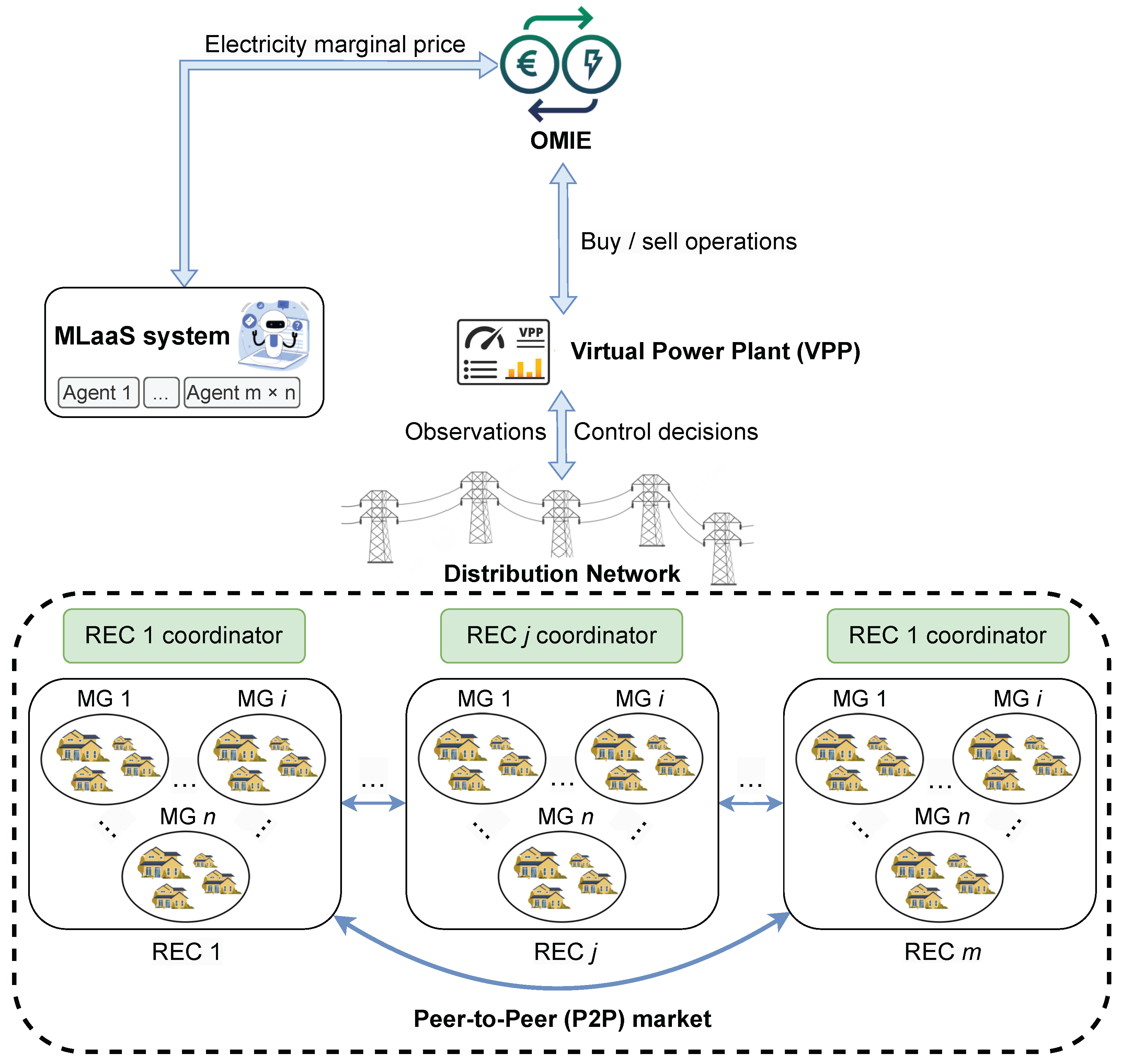
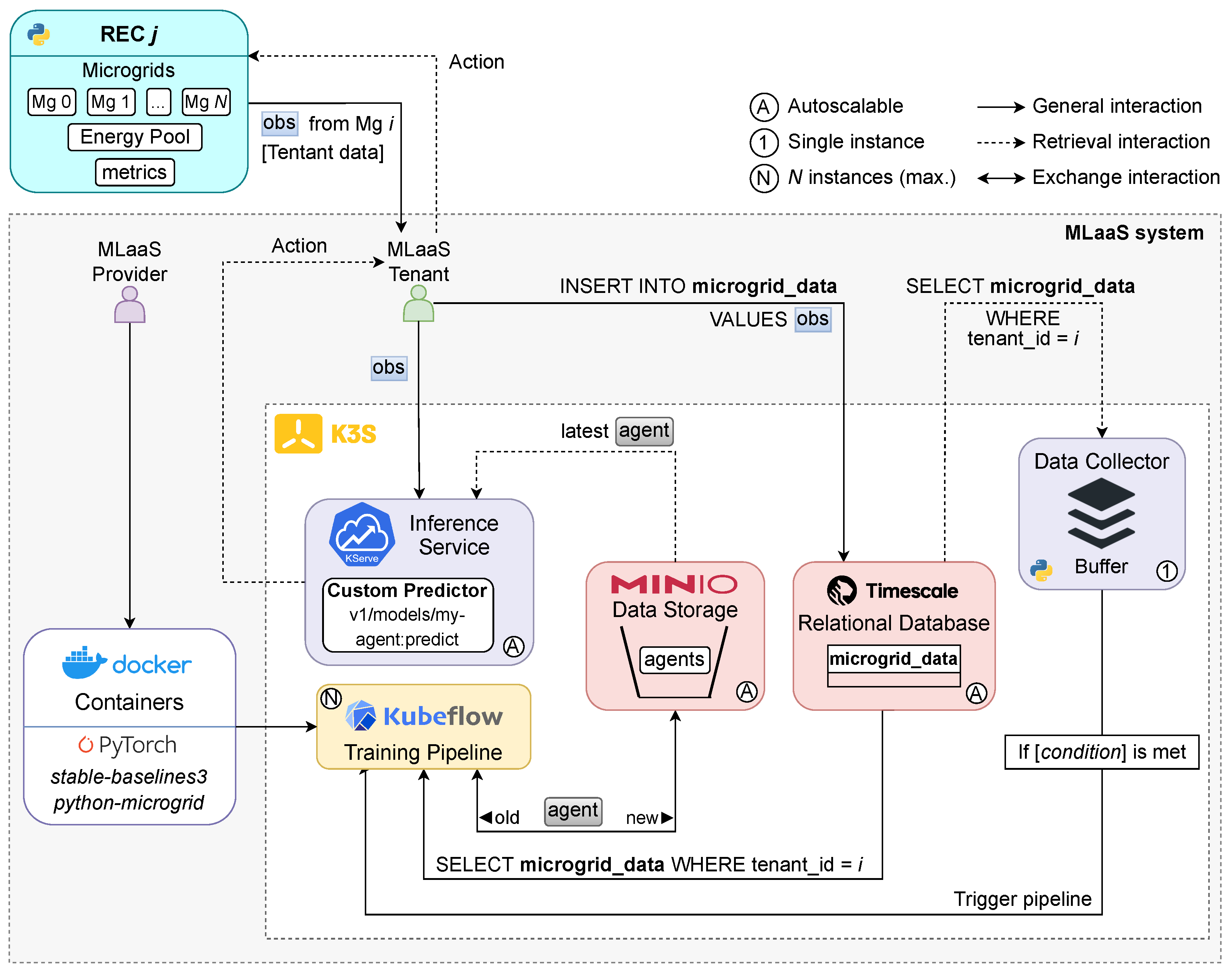
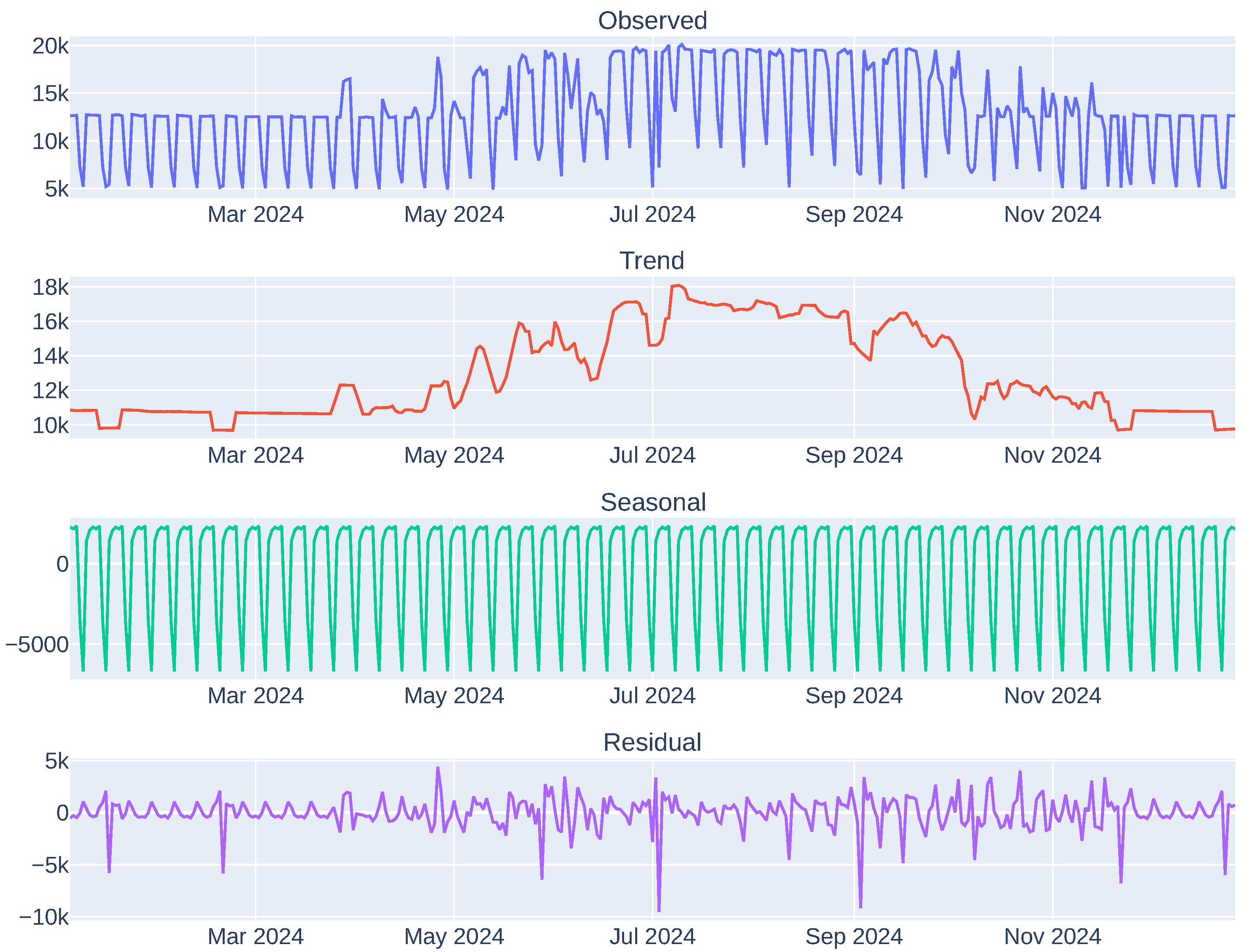
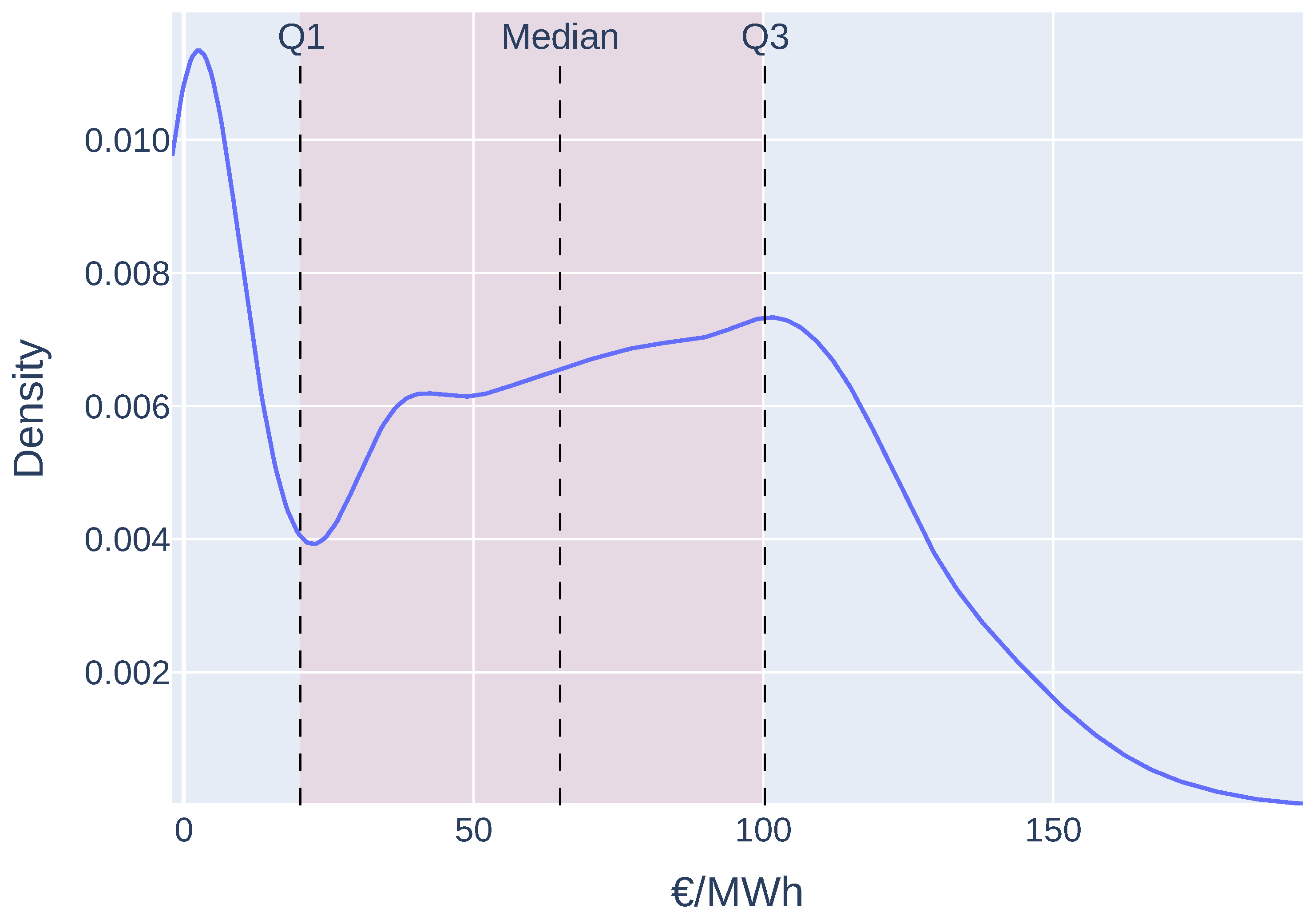
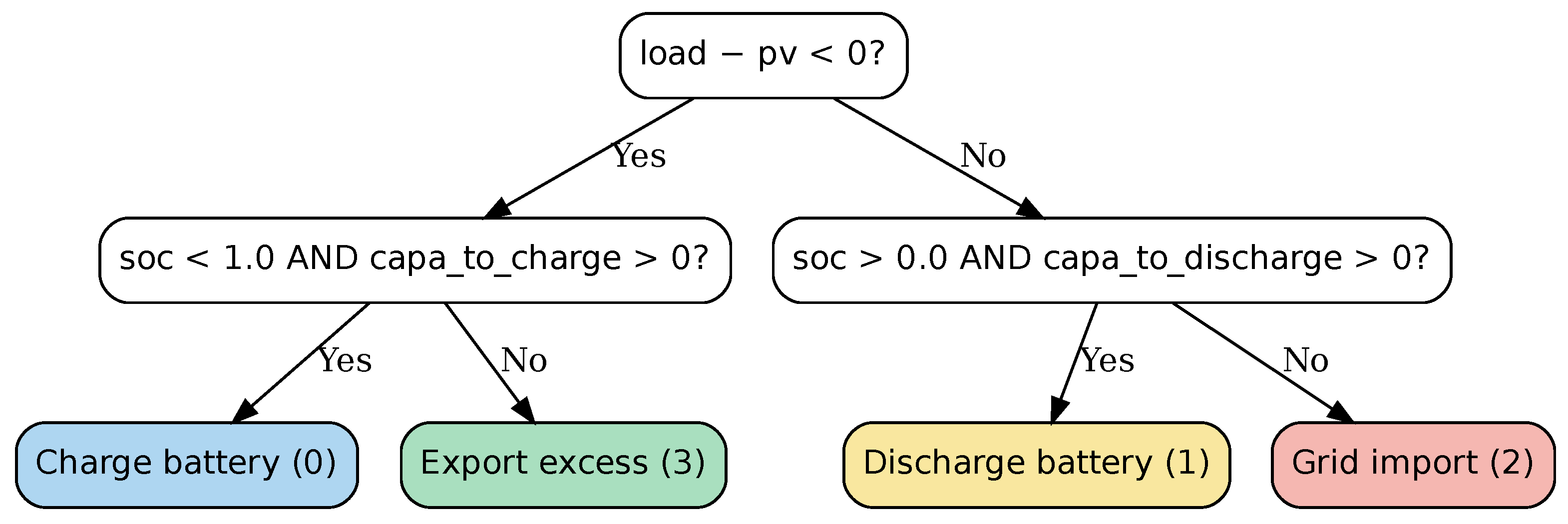
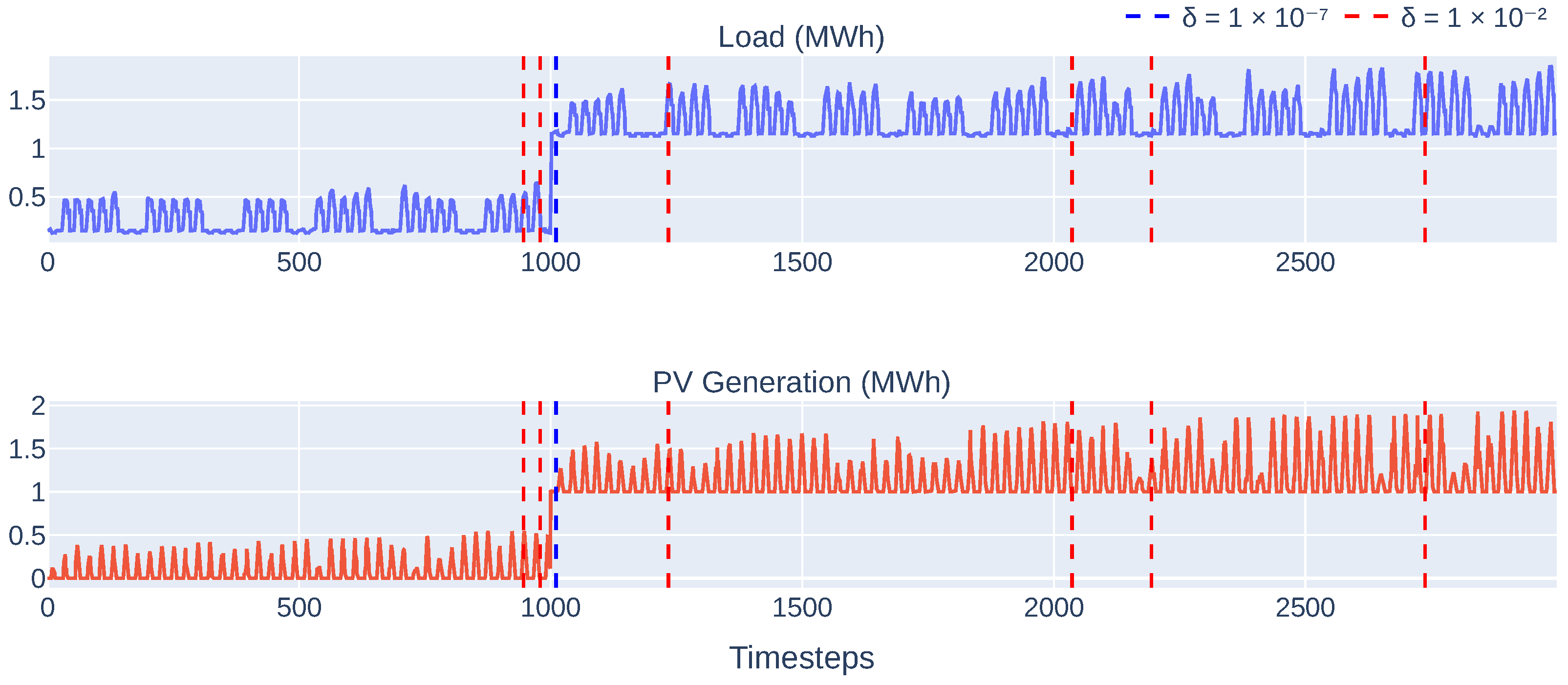
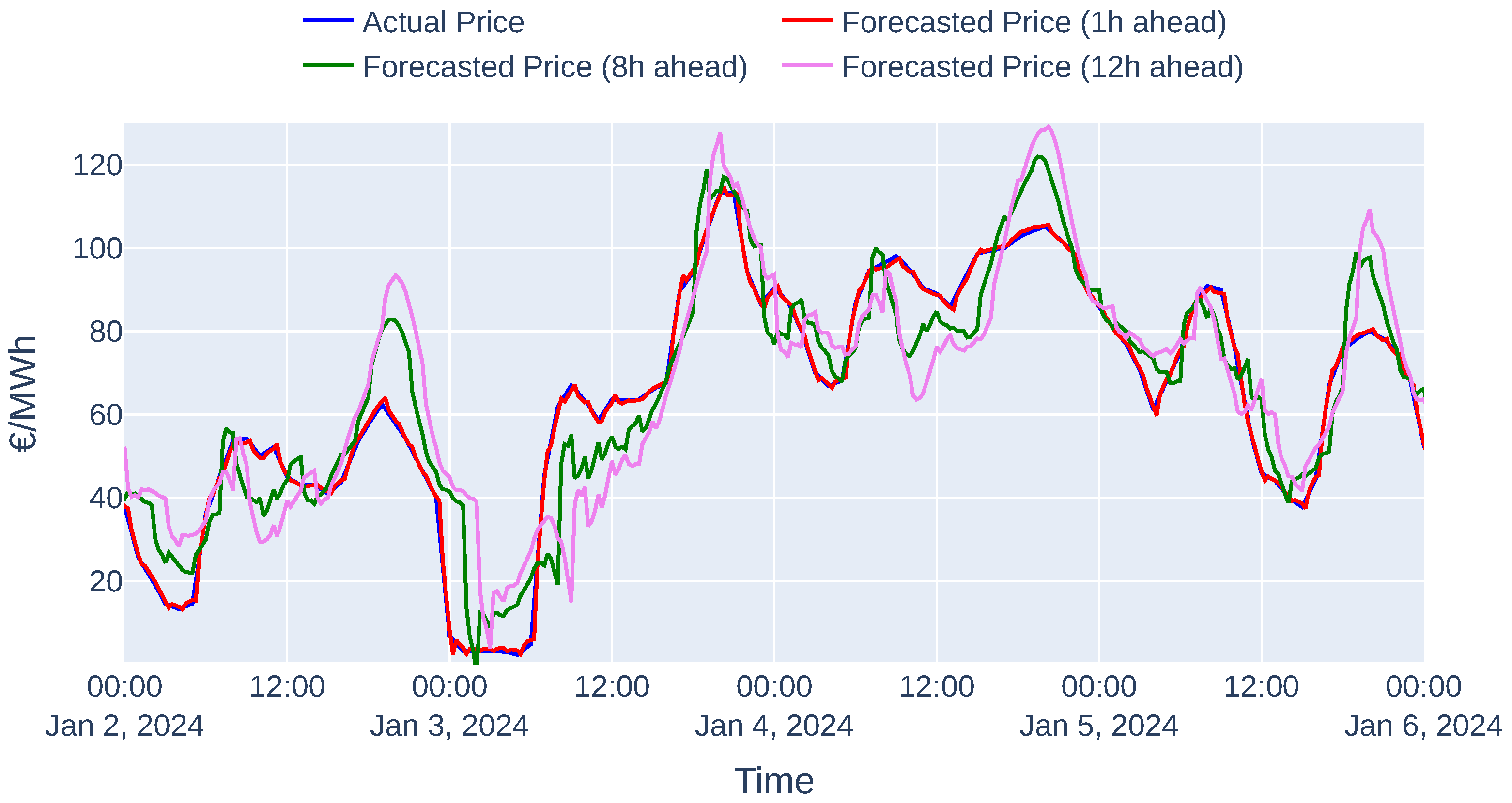
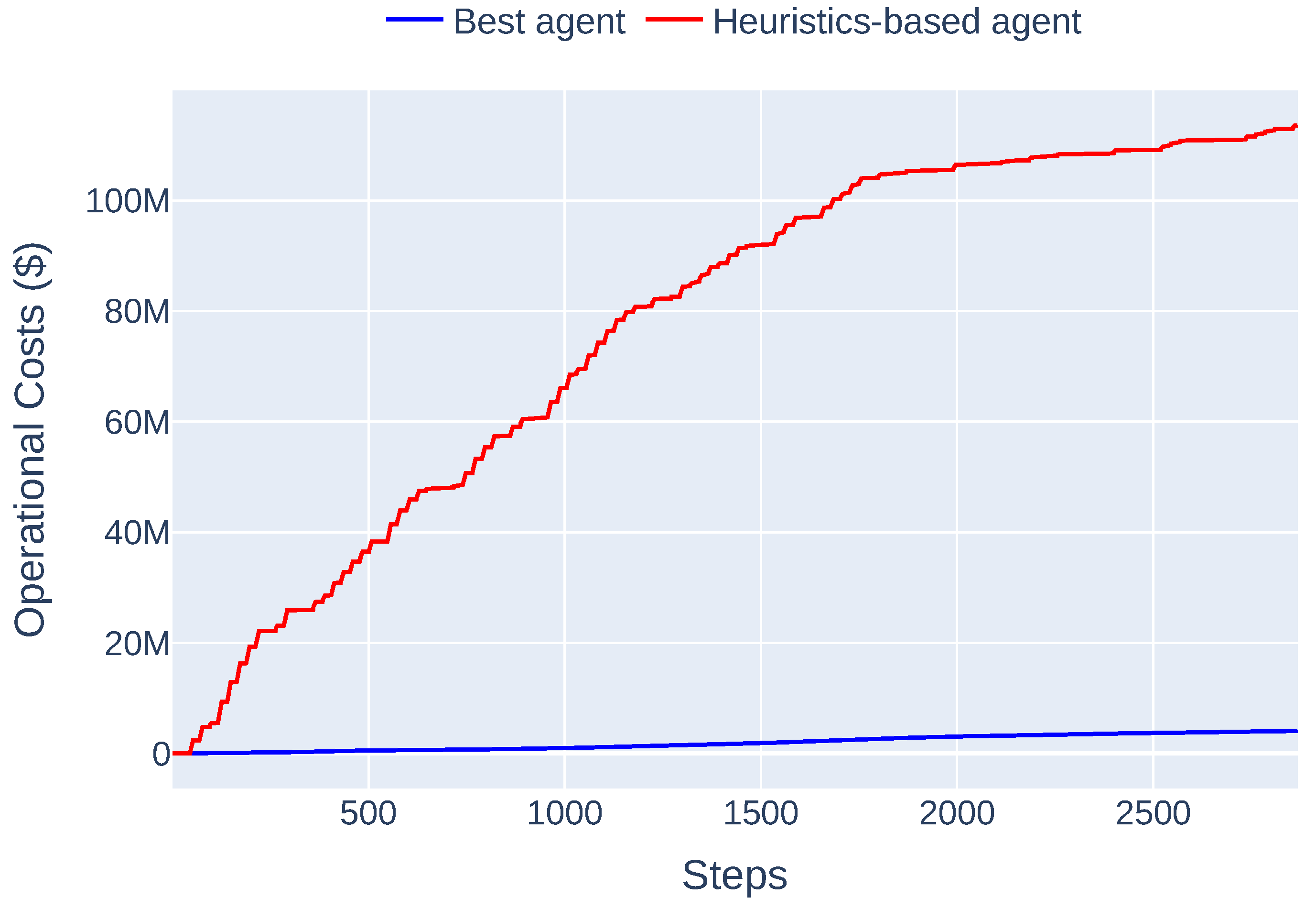
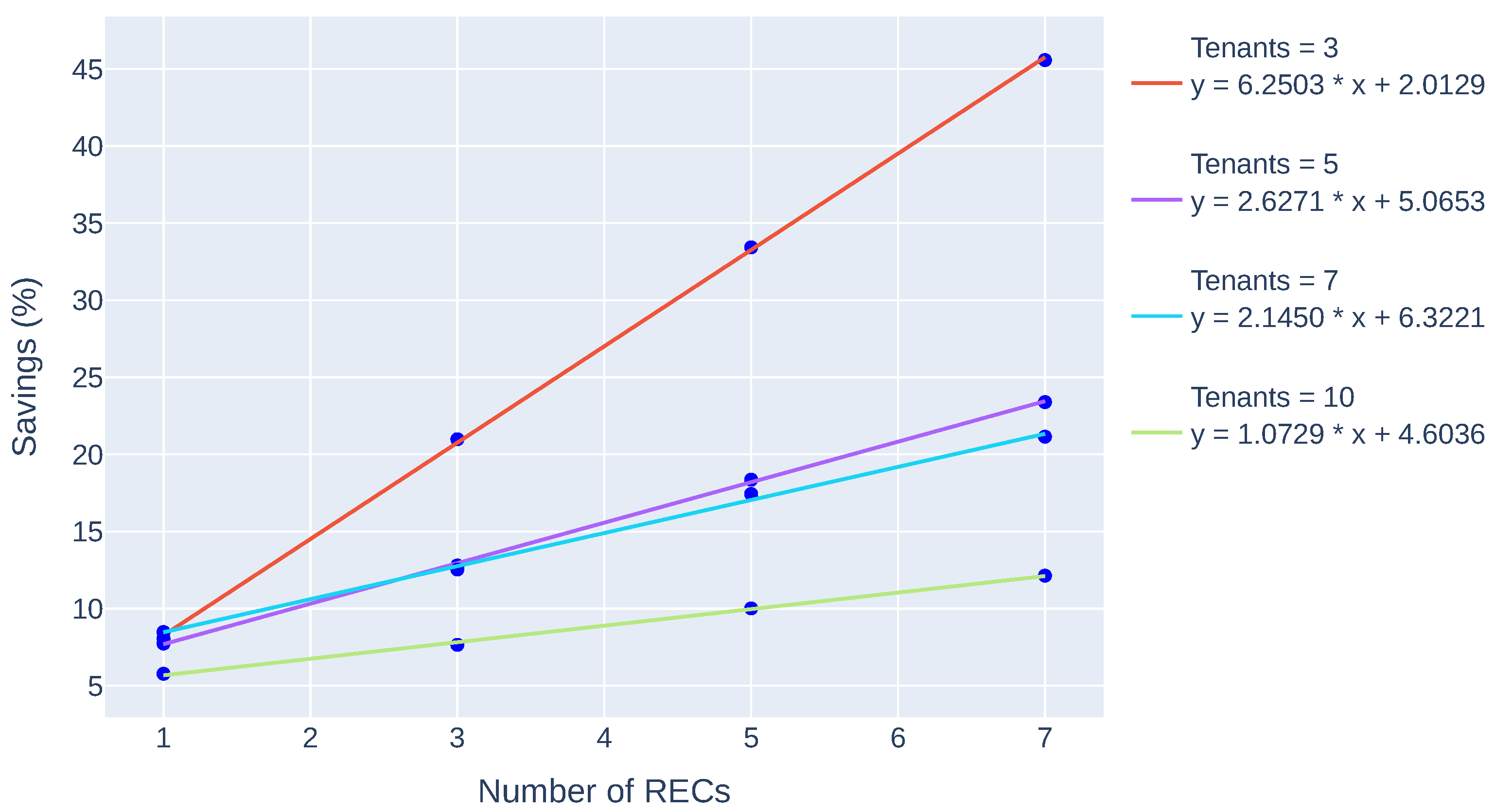
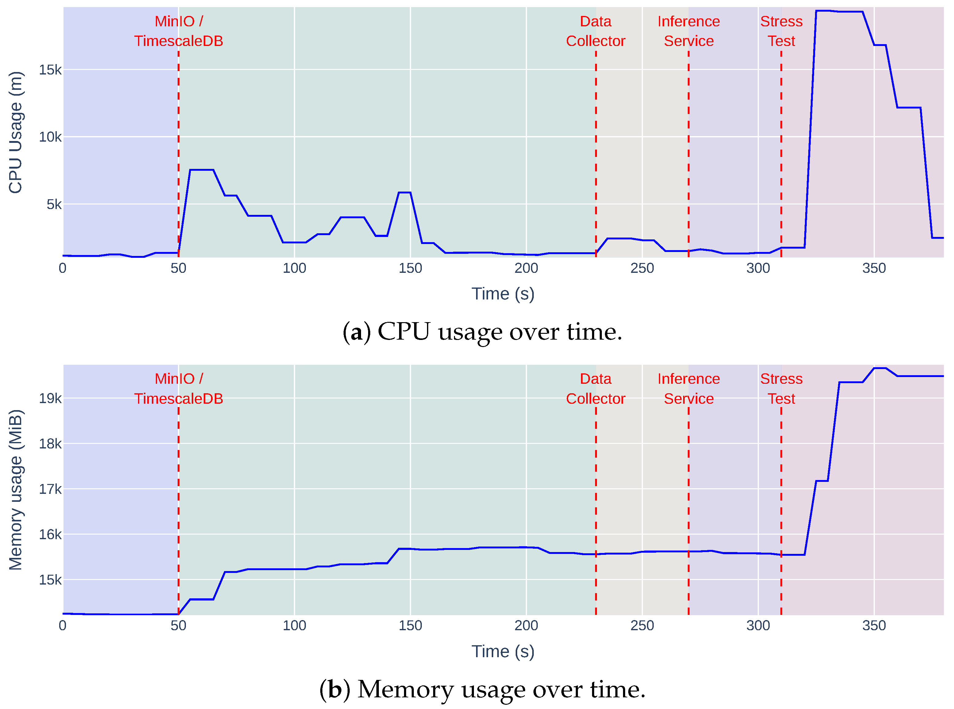
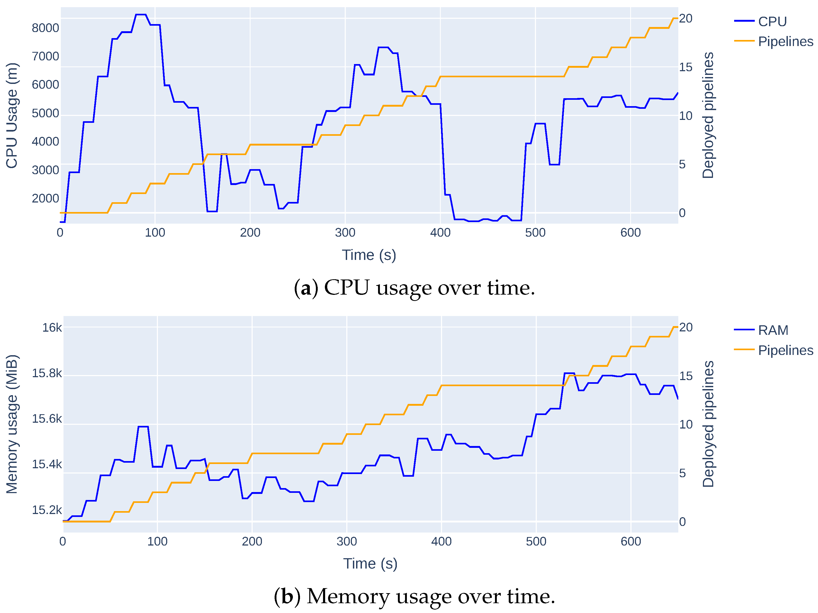
Disclaimer/Publisher’s Note: The statements, opinions and data contained in all publications are solely those of the individual author(s) and contributor(s) and not of MDPI and/or the editor(s). MDPI and/or the editor(s) disclaim responsibility for any injury to people or property resulting from any ideas, methods, instructions or products referred to in the content. |
© 2025 by the authors. Licensee MDPI, Basel, Switzerland. This article is an open access article distributed under the terms and conditions of the Creative Commons Attribution (CC BY) license (https://creativecommons.org/licenses/by/4.0/).