Abstract
The virtual synchronous generator (VSG) scheme has proven to be an attractive solution in grid-forming converter applications integrated into distributed generation (DG) systems. Thus, this paper presents the dynamic performance of power flow control using the VSG approach under Thevenin impedance variations seen by the grid-forming converter. The dynamic analysis is based on a discrete-time model that describes the power flow transient characteristics of the system operating in medium- and high-voltage networks. Based on the proposed model, a controller design procedure for the discrete-time VSG scheme is presented. This methodology aims to assist researchers in implementing VSG control in digital environments. Then, the Thevenin impedance parameters’ influence on the discrete-time VSG strategy dynamic performance is discussed. The VSG technique’s performance in different operating scenarios is assessed by means of simulation results. A case study is provided to validate the effectiveness of the theoretical analysis and the discrete-time VSG control scheme. The results assess the effectiveness of the theoretical analysis performed.
1. Introduction
Grid-forming DG systems based on renewable energy sources (RESs) are typically interfaced to the grid through DC–AC power converters equipped with output filters. These systems operate as controlled voltage sources while also providing ancillary services to the grid [1]. In this paradigm, DG units can actively regulate the power exchanged with the grid, similar to conventional synchronous generators (SGs) [2]. However, this operating mode poses significant challenges in terms of dynamic response and system stability, primarily due to the lack of inherent inertia and damping in converter-based interfaces [3]. To address these issues, various control strategies have been proposed to enhance the power regulation capability of DG units. Among these, the virtual synchronous generator (VSG) technique has gained considerable attention due to its ability to replicate the dynamic behavior of conventional SGs [4,5,6,7,8,9,10,11]. By emulating inertia and damping characteristics, the VSG approach enhances transient stability and improves dynamic performance in power systems.
In general, the implemented VSG scheme assumes that the Thevenin impedance is predominantly inductive, which is common in high- and medium-voltage systems. However, in low-voltage systems, the Thevenin impedance is predominantly resistive [1], which can compromise the performance of the VSG technique. An alternative to this problem is to design a virtual inductance so that the Thevenin impedance becomes predominantly inductive [12].
The VSG control gains can be designed using dynamic performance and stability criteria. Consequently, some methods of dynamic analysis and the design of parameters based on small-signal models for VSG-controlled DG systems have been discussed in the literature [13,14,15,16,17,18,19,20]. These analyses enable prediction of dynamic behavior under parameter variations, providing valuable insights for optimal tuning of control gains.
In [13], the proposal was to perform a dynamic analysis of the VSG scheme based on the DG active power flow modeling, addressing the system’s stability analysis and control gains design. However, the proposed analysis does not address the reactive power control loop. Moreover, the controller design did not account for desired performance requirements, resulting in control parameter tuning through trial-and-error procedures. To overcome these limitations, subsequent studies [14,15,16,17,18] proposed more comprehensive analyses incorporating both active and reactive power flow models. These works decoupled the active and reactive power control loops by assuming specific transient performance requirements, thereby enabling independent tuning of the VSG controllers. However, these analyses were based on dynamic models that reflect only steady-state power flow, introducing uncertainty in the evaluation of the controller dynamic performance and often requiring adjustments of post-design parameters. Thus, a more realistic dynamic modeling approach is still required for accurate VSG controller design. In this context, a more rigorous analysis based on detailed DG power flow modeling was proposed in [19], where the frequency response method was used to investigate the closed-loop system behavior under variations in the VSG control parameters, offering valuable insights for improved controller tuning.
The dynamic analysis of the VSG strategy is based on system power flow modeling, which depends on the system’s Thevenin impedance. This impedance may vary due to changes in load and generation within the power system. Therefore, evaluating the VSG control performance under variation in the Thevenin impedance is essential. However, the dynamic behavior of the VSG scheme has not been thoroughly investigated in scenarios where Thevenin impedance parameters deviate from their nominal values. A dynamic analysis of VSG controller performance, incorporating DG power flow modeling that accounts for the transient characteristics of the impedance, was proposed in [20]. This analysis established the relationship between the DG power flow dynamic response and Thevenin impedance variations, providing a foundation for the design of VSG control gains.
In the works above, the VSG scheme parameter design is based on continuous-time system modeling. In such cases, the designed controllers can be discretized using bilinear transformations to emulate the continuous-time dynamic behavior in a digital environment [21]. However, the accuracy of the bilinear transformation depends on the sampling time used and may result in significant discrepancies between the controller performance in continuous and discrete time domains. The design of a discrete-time VSG scheme, suitable for accurately representing time delays and enabling direct digital implementation, was proposed in [22,23]. In [22], an RLM-based VSG controller parameter design method was introduced, employing transient response specifications derived from discrete-time mathematical modeling that accounts for the transient characteristics of the Thevenin impedance. This approach ensures precise achievement of the desired dynamic response. Subsequently, an observer-based state-feedback VSG control strategy was proposed in [23], where the discrete-time controller design was based on system identification and model-matching techniques. This methodology offers a unified and systematic framework for implementing and tuning VSG control gains. However, the dynamic performance of the discrete-time VSG control strategy has not yet been investigated under variations in Thevenin impedance, which may result from changes in system loads or generation units. Furthermore, while the VSG strategy can operate in either reactive power support or voltage support modes, the design methodologies proposed in [22,23] address only the reactive power support mode. Therefore, this paper conducts a dynamic analysis considering grid impedance variations and proposes a control parameter design for both operating modes of the VSG strategy. The main contributions of the paper are summarized as follows:
- Based on a discrete-time power flow model, discrete-time active and reactive power controllers are designed to achieve the desired dynamic response in both the reactive power support and voltage support operating modes of the VSG strategy. The proposed design method can be used as a useful design guideline for the implementation of the VSG scheme in a digital environment.
- The behavior of the closed-loop poles and their sensitivity to VSG control gains are discussed, considering the effect of the system’s equivalent impedance variations and variations in the sampling time.
This paper organizes the sections as follows. Section 2 presents the description and modeling of the VSG-based DG system used in this work. Section 3 and Section 4 introduce the discrete-time VSG control scheme and its proposed discrete-time parameter design method. Section 5 presents closed-loop pole behavior under parametric variations. The simulation results for performance assessment are given in Section 6, while Section 7 concludes this paper.
2. System’s Description and Modeling
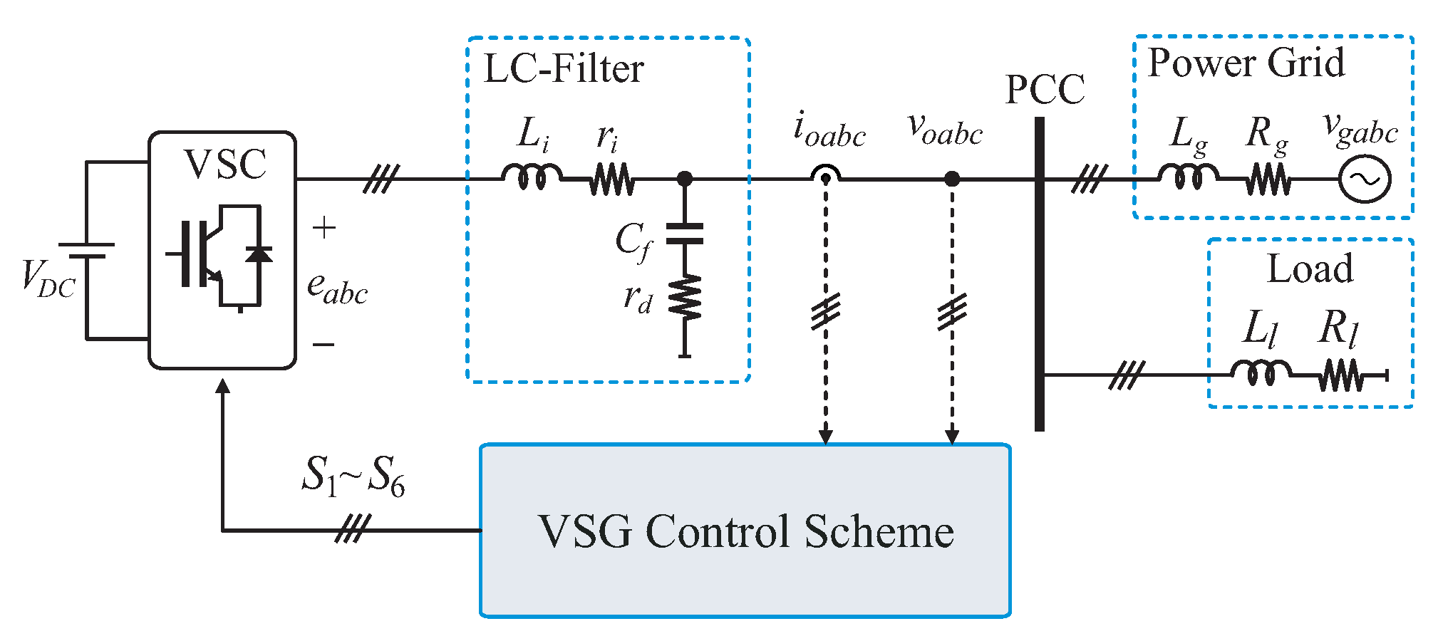
Figure 1 illustrates the grid-forming DG system topology employed in this study. The system consists of a conventional three-phase two-level voltage source converter (VSC) connected to the point of common coupling (PCC) through an LC filter, which includes the converter-side inductor , filter capacitor , and damping resistor . The term represents the winding resistance of the inductor . A DC voltage source models the primary energy source of the converter. The power grid is represented by a three-phase sinusoidal voltage source in series with a grid impedance composed of the inductor and resistor . Additionally, a three-phase load is connected at the PCC, modeled by an inductor and resistor .
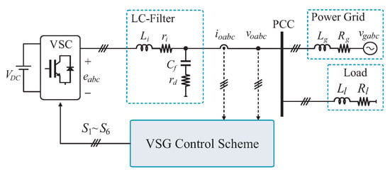
Figure 1.
Block diagram of the grid-forming DG system.
Considering the balanced three-phase system, it is possible to represent the grid-forming DG system with the equivalent circuit shown in Figure 2. In this circuit, the grid-forming converter operates as a controllable voltage source connected to the PCC [1], the inductor and resistor represent the Thevenin impedance seen by the DG unit, and and represent the active and reactive power delivered to the power grid. In general, the Thevenin impedance can be determined through system load flow analysis or by employing impedance estimation techniques [24,25].
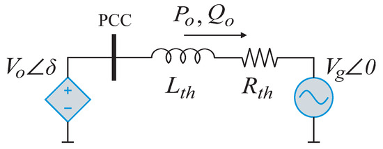
Figure 2.
Equivalent circuit of the grid-connected DG unit.
In medium- and high-voltage systems with a range of 1–100 kV and 100–230 kV, respectively [26], the Thevenin impedance is predominantly inductive, where the power flow model describes the relationships between active power () and instantaneous load angle (), as well as between reactive power () and voltage amplitude () [20]. Thus, a dynamic model that describes the DG active power flow transient behavior can be given by:
in which
The term is the nominal load angle value, while and are the nominal values of the PCC voltage and the grid, respectively. is the grid frequency. Thus, considering any sampling time T, the active power discrete-time model is achieved by applying the z-transform to the transfer function cascaded with a zero-order hold as [21]:
which results in the following expression
where
The dynamic model that characterizes the direct relationship between reactive power and variations in the VSC output voltage is [20]:
in which
By applying the z-transform to the transfer function in cascade with a zero-order hold, the reactive power discrete-time model can be obtained as follows:
in which
3. Discrete-Time VSG Control Scheme
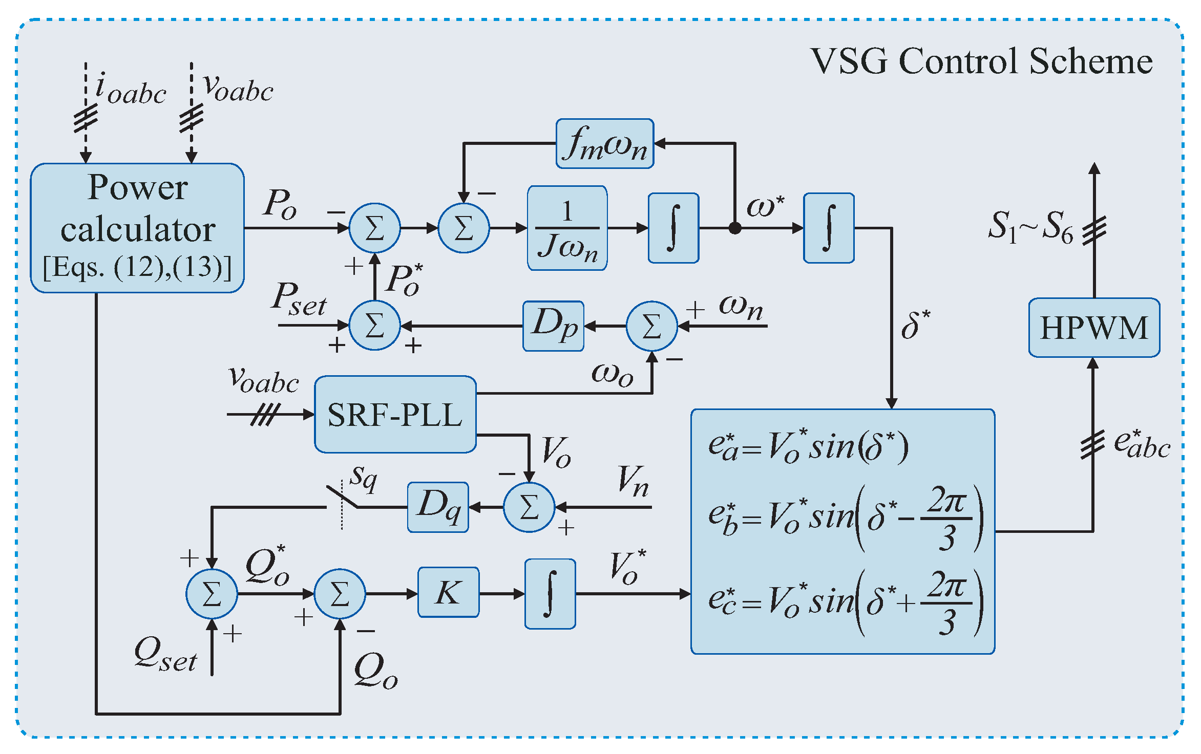
Figure 3 illustrates the VSG control strategy, which consists of active and reactive power control loops. The instantaneous active () and reactive () power values used as feedback in the outer control loops are computed using the following expressions [27]:
in which , , and are PCC voltages, while , , and represent currents delivered to the power grid.
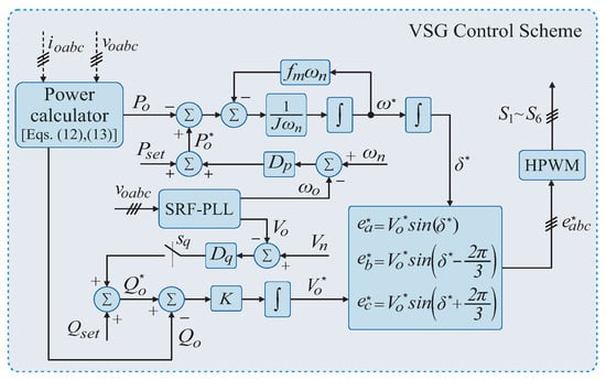
Figure 3.
Block diagram of the VSG control scheme.
According to Figure 3, the VSG scheme adjusts the active and reactive power values according to the transient frequency and voltage variations at the PCC, respectively. Thus, the active and reactive power reference values are calculated as:
where and represent active and reactive power nominal values, respectively. and are frequency and voltage amplitude estimates provided by a synchronous reference frame phase-locked loop (SRF-PLL), and are the system’s nominal frequency and voltage, and and represent droop gains. In this case, the reference value for the reactive power depends on the states of ( corresponds to being off and to being ON). Thus, if , the DG reactive power flow control operates in voltage support mode, which results in a divergence between and , while the difference between and is reduced. On the other hand, if , the DG reactive power flow control operates in the reactive power support mode, resulting in tracking by without steady-state error, while and diverge.
The VSC output voltage reference is computed based on the instantaneous voltage amplitude , determined by the reactive power control loop, and the phase angle , provided by the active power control loop. Subsequently, the hybrid pulse width modulation (HPWM) strategy generates the gate drive signals for the power switches [28].
3.1. Discrete-Time Active Power Controller
In the VSG control scheme, the active power controller emulates the mechanical motion equation of a conventional SG to introduce virtual inertia and damping characteristics, which results in control laws given by:
in which represents the active power error. The terms J and represent the inertia moment and the friction factor, respectively.
Considering small disturbances around the system’s operating point yields the following expressions:
in which , , and represent operating point values, while , , and are small ac variations.
The expression in (20) neglects the constant terms associated with the system’s operating point. By integrating the frequency deviation, the load angle can be obtained as follows:
Finally, by applying the Laplace transform to (20) and (21), a small-signal model for the VSG active power controller can be derived as:
The controller model given in (22) features a pole at the origin, enabling to track without steady-state error. Applying the z-transform to (22) yields the discrete-time model of the VSG active power controller, given by:
in which
represent the discrete-time active power controller gains. Accordingly, the controller coefficients are computed based on the inertia moment and friction factor defined in the continuous-time (s-domain) model, as described in (24) and (25).
The VSG active power controller given in (23) can be implemented in a digital environment using the following difference equation:
where represents the controller input and is the controller output. Thus, the current output sample depends on past input samples as well as past output samples. Figure 4 depicts the flowchart of the active power controller, which can be used to develop a program for its digital implementation.
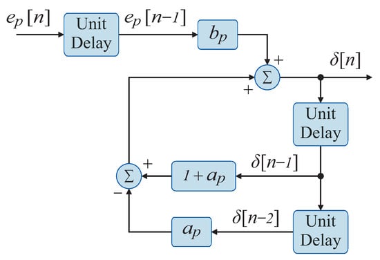
Figure 4.
Flowchart of the discrete-time active power controller.
3.2. Discrete-Time Reactive Power Controller
The VSG reactive power controller, as shown in Figure 3, operates based on the following control law:
in which K is the integral gain.
The expression in (27) can be linearized by assuming small perturbations around the system’s operating point given by:
where , , and represent the operating point values, while , , and denote small-signal variations. Assuming and substituting (28)–(30) into (27) yields the following expression:
in which constant terms associated with the system’s operating point are neglected. Applying the Laplace transform to (31) yields the small-signal model of the VSG reactive power controller, given by:
According to (32), the controller structure described in (32) depends on the state of . Thus, for , the controller has a pole at the origin, and is accurately tracked by . However, if , the controller has a pole on the real axis, which results in a steady-state error proportional to the .
Applying the z-transform to (32) yields the discrete-time model of the reactive power controller, given by:
in which
represents a control gain that depends on the VSG control strategy operation mode. Thus, the difference equation used to implement the reactive power controller is given by:
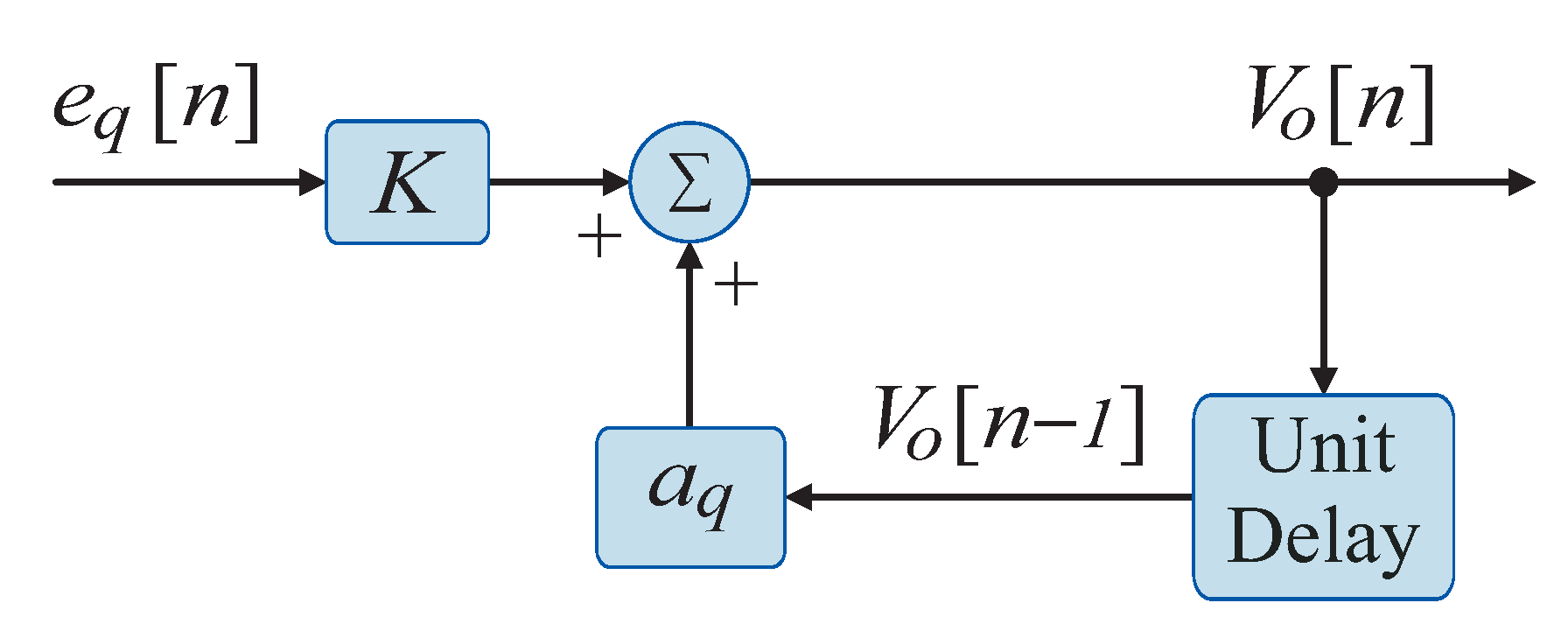
where the reactive power error serves as the controller input, and the controller output corresponds to . In this case, the output at each sample instant is a function of past output samples as well as the current input sample. Figure 5 shows the flowchart of the reactive power controller.
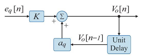
Figure 5.
Flowchart of the discrete-time reactive power controller.
4. VSG Controller Parameter Design
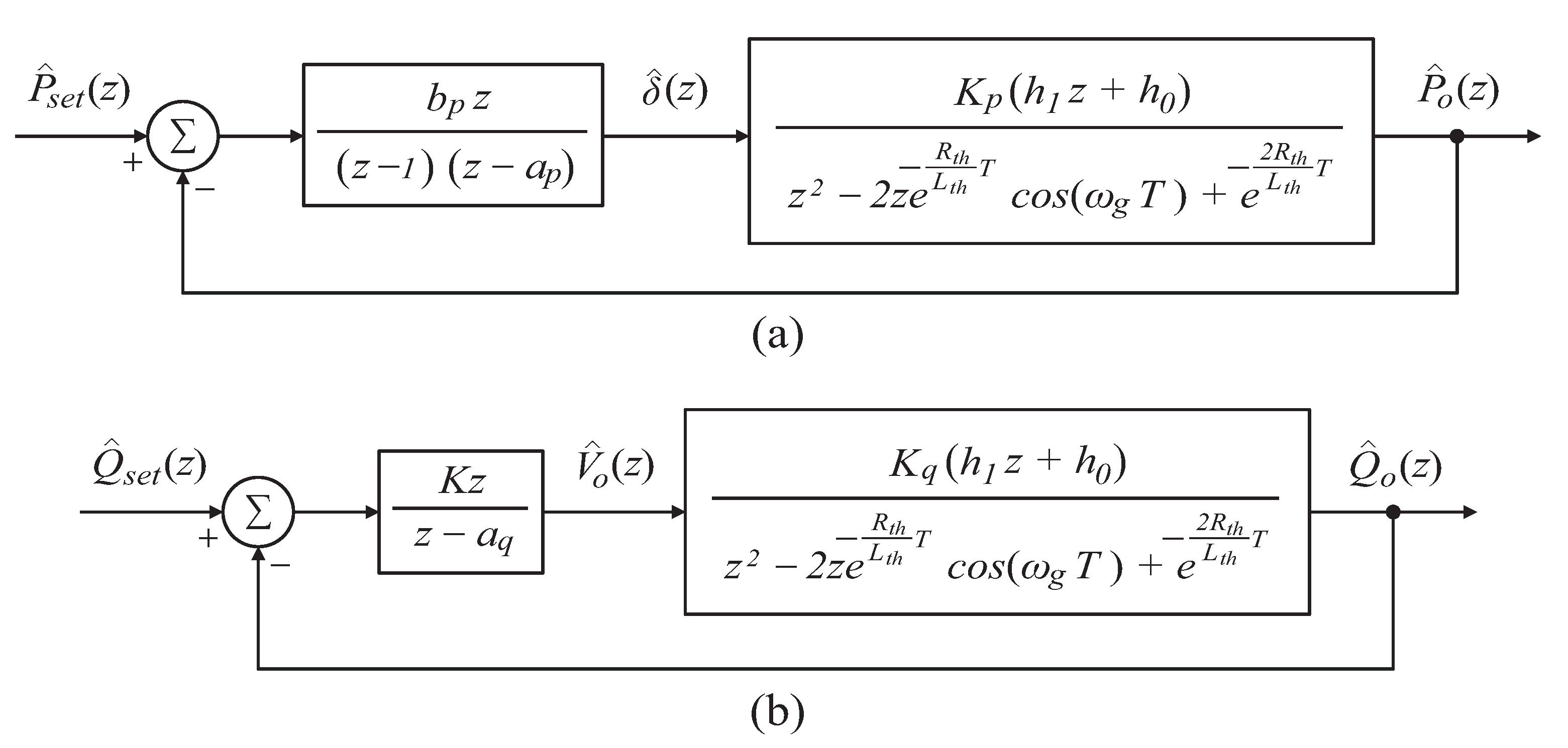
This section describes the methodology used for designing the active and reactive power controllers of the VSG strategy. Figure 6 shows the equivalent block diagram of the DG active and reactive power control loops. The design procedure is based on the RLM and utilizes the system parameters listed in Table 1. In addition, the sampling time T was set as equal to the converter switching period for both power control loops.
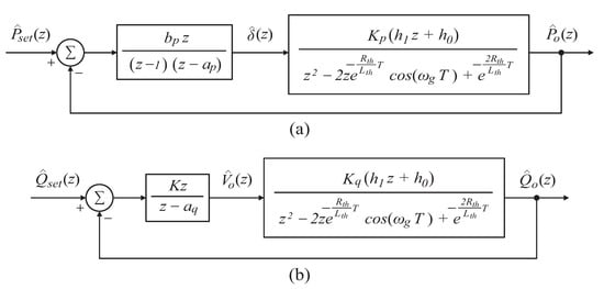
Figure 6.
Equivalent block diagram of the (a) active power control loop and (b) reactive power control loop.

Table 1.
DG system parameters.
4.1. Active Power Controller Design
The active power controller design, as shown in Figure 6a, is based on the discrete-time model given in (4) and the controller model described in (23), resulting in the following open-loop transfer function:
In this work, the performance requirements for the active power controller design were established to ensure a well-damped dynamic response, free from significant oscillations. Thus, considering the performance requirements of percent overshoot () less than or equal to 10% and settling time () less than or equal to s, the minimum values of natural frequency () and damping ratio () for the closed-loop active power control are calculated as follows [21]:
in which results in the desired closed-loop pole given by:
where
According to the RLM, the gain is determined using the angle restriction, resulting in the following expression:
in which
The solution of the expression in (41) ensures that the desired closed-loop poles lie on the root locus; however, their exact placement is achieved by applying the magnitude restriction, which is used to compute the gain , as expressed by:
According to (39), (41), and (43), the computation of the control gains depends on both the design specifications and the sampling time. Based on the desired performance criteria and the parameters listed in Table 1, the active power controller gains are calculated and presented in Table 2. The resulting root locus of the active power loop is shown in Figure 7. The closed-loop system exhibits four complex poles located within the unit circle in the z-plane, ensuring system stability. Among them, the two dominant poles correspond to the desired location , while the remaining non-dominant poles are located further from the unit circle.
Table 2.
VSG controller parameters.
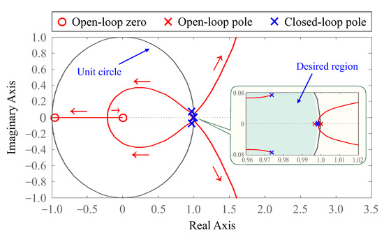
Figure 7.
Closed-loop poles for DG active power control in the z-plane.
4.2. Reactive Power Controller Design
The reactive power control loop utilizes the discrete-time model given in (10) and the discrete-time controller described in (33), as shown in Figure 6b. Accordingly, the open-loop transfer function is obtained as follows:
The performance requirement for the reactive power controller is defined as s, which leads to the condition . Based on this specification, the desired closed-loop pole is determined as:
In this case, the calculation of the gain K is based on the magnitude restrictions, resulting in the following expression:
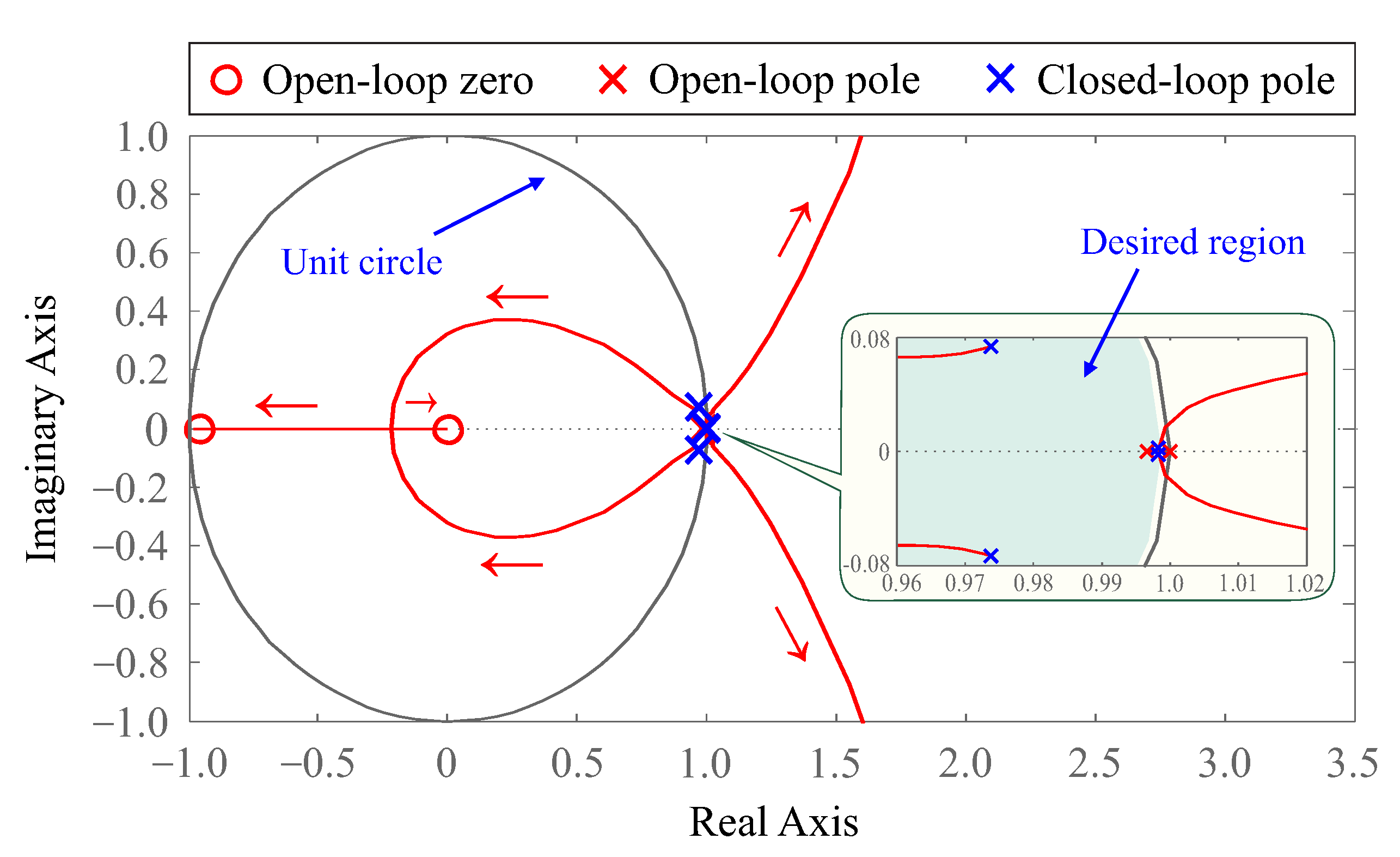
For operation in reactive power support mode, is equal to zero, which results in . On the other hand, if the VSG strategy operates in the voltage support mode, that is, , the value of can be chosen to satisfy the transient response requirement and to allocate the closed-loop poles within the desired region in the z-plane. Reactive power control gains are configured as listed in Table 2. Figure 8 illustrates the location of the closed-loop poles for VSG reactive power control in the z-plane. For both modes of operation, the control loop exhibits three closed-loop poles located within the desired region of the unit circle. The real dominant pole corresponds to , whereas the remaining complex conjugate poles are non-dominant and positioned closer to the boundary of the unit circle. In addition, for the reactive power support mode, the system exhibits an open loop pole on the unit circle, as shown in Figure 8a, which ensures zero steady-state error. Conversely, in voltage support mode, the open-loop poles are located inside the unit circle, as depicted in Figure 8b, resulting in a nonzero steady-state error.
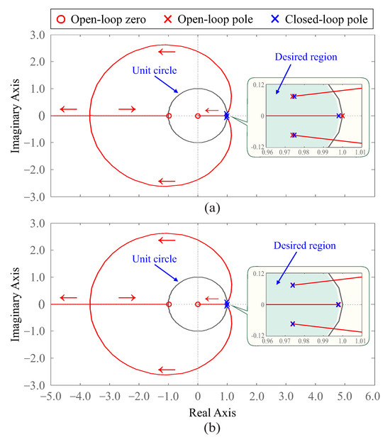
Figure 8.
Closed-loop poles for DG reactive power control in the z-plane when (a) and (b) .
5. VSG-DG Power Control Dynamic Analysis
This section describes a dynamic analysis for closed-loop power control considering the discrete-time models of active and reactive power discussed in Section 2 and the discrete-time VSG controllers described in Section 3. The proposed analysis uses the parameters of the DG system listed in Table 1 and the control parameters given in Table 2.
5.1. Closed-Loop Poles Behavior
5.1.1. Active Power Loop
From the model given in (4) and the controller described in (23), it is possible to obtain the closed-loop transfer function related to active power control as:
in which
represent the coefficients of the characteristic polynomial for an active power control loop.
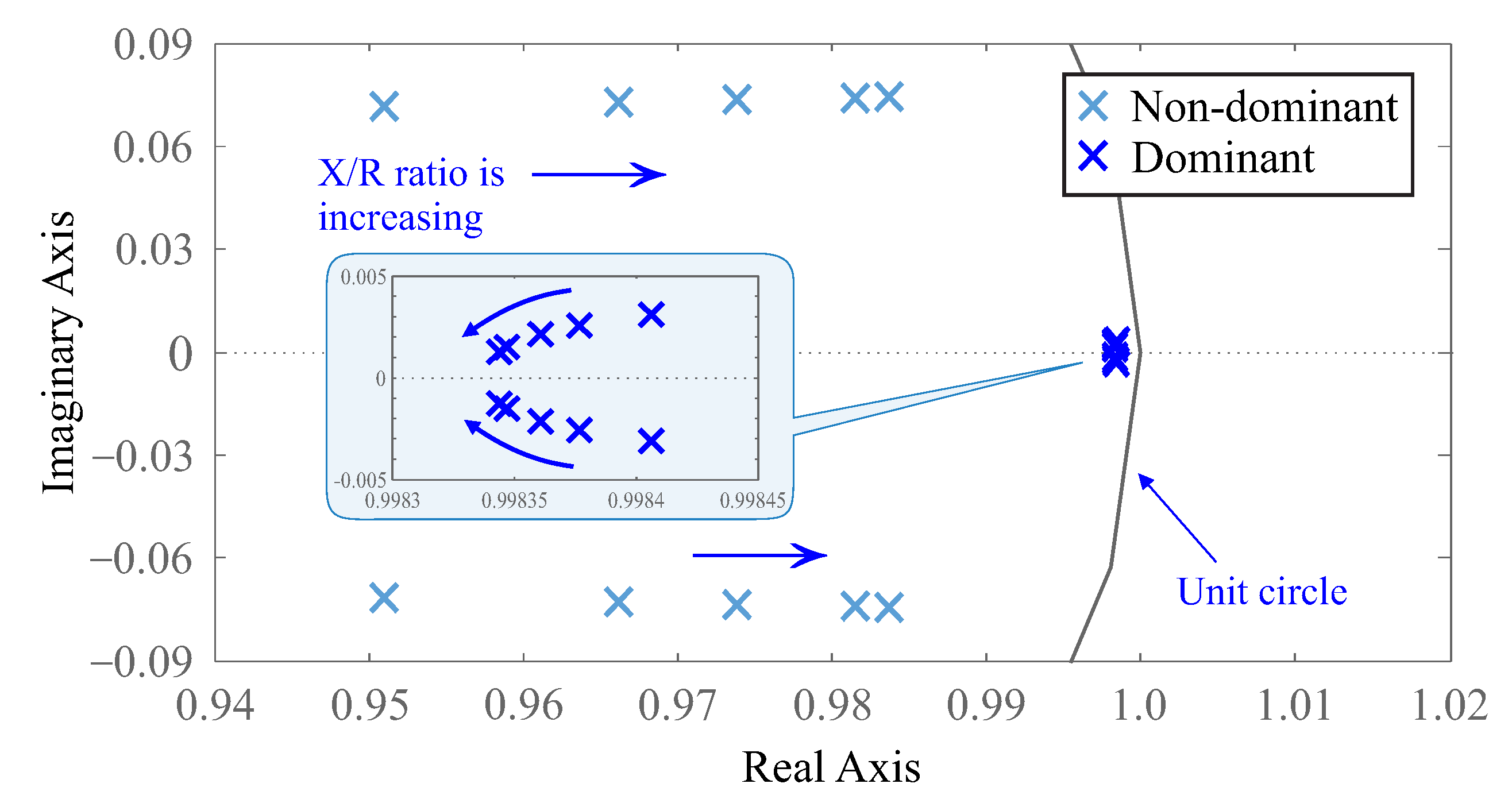
Figure 9 shows the behavior of the closed-loop poles of active power control during variations in the ratio between 1.6 and 5.5. The closed-loop system has four complex poles. Two dominant poles closer to the unit circle and two complex non-dominant poles farther to the unit circle. As the ratio increases, the dominant poles are closer to the real axis, which can contribute to a less oscillatory dynamic performance. On the other hand, the non-dominant poles are closer to the unit circle, which increases its contribution to the system’s dynamic performance, resulting in a more oscillatory transient behavior.
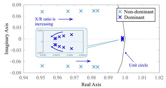
Figure 9.
Active power control closed-loop poles when the ratio varies.
5.1.2. Reactive Power Loop
The closed-loop transfer function for reactive power control employs the model given in (10) and the controller described in (33), which results in:
in which
represents the coefficients of the characteristic polynomial for the reactive power control loop.
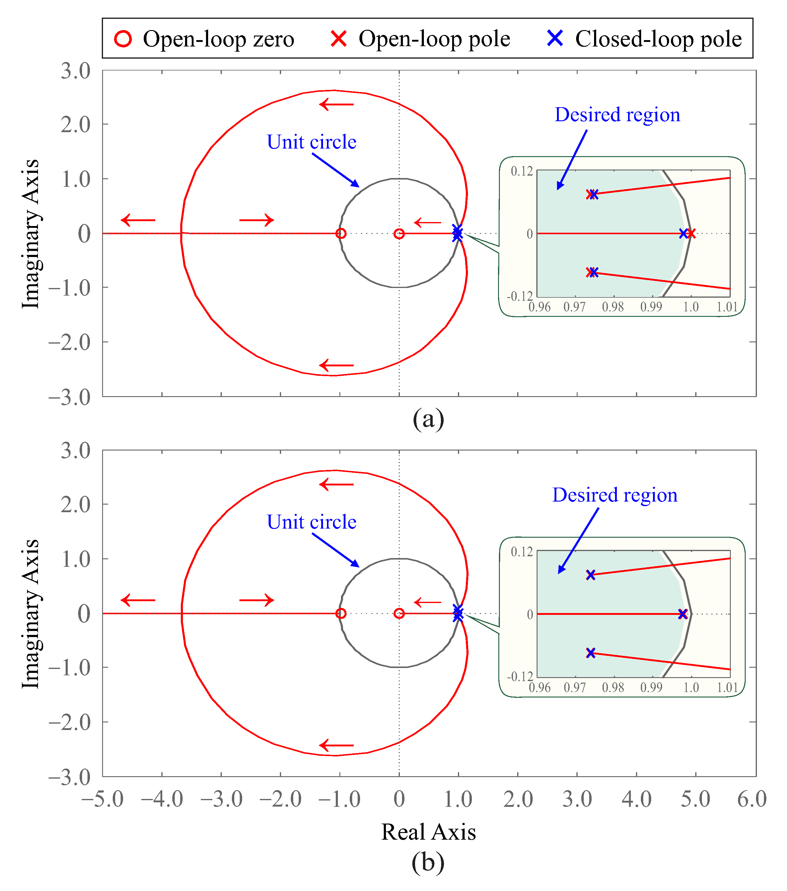
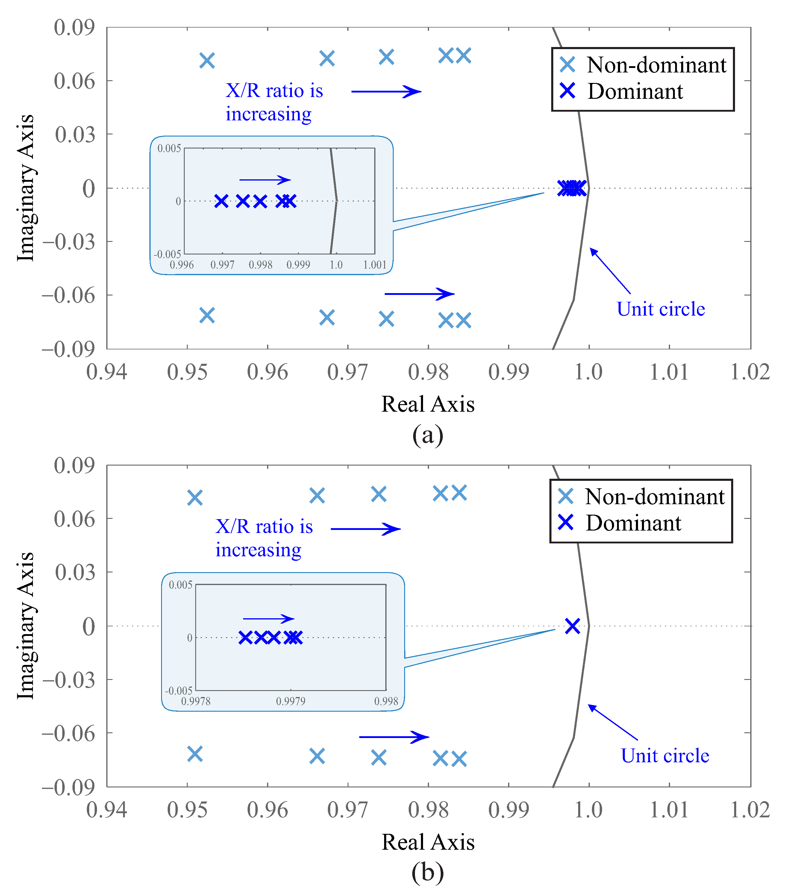
Figure 10 shows the behavior of the closed-loop poles of the reactive power control under variation in the ratio for the reactive power and voltage support mode. In both operating modes, the reactive power control has one real dominant closed-loop pole that guarantees the desired performance and two complex non-dominant closed-loop poles furthest to the unit circle. When the ratio increases, all poles are closer to the unit circle, resulting in a slower transient response. However, the dominant pole for the case of the voltage support mode showed less variation in its location during the variation of the ratio.
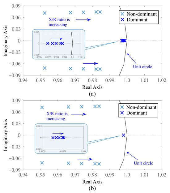
Figure 10.
Closed-loop poles of the reactive power control when the ratio varies. (a) Reactive power support mode; (b) voltage support mode.
5.2. Sensitivity Analysis
Using the sensitivity analysis, it is possible to describe the effect of variations in the ratio on the sensitivity of the closed-loop poles in relation to a control gain [21]. Then, by differentiating the denominator of (47) with respect to , it is possible to obtain the sensitivity of a closed-loop pole, z, to gain, , given by:
Adopting a similar procedure, the sensitivity of a closed-loop pole, z, to gain, K, can be obtained from the derivative of the denominator of (52) with respect to K, which results in the following expression:
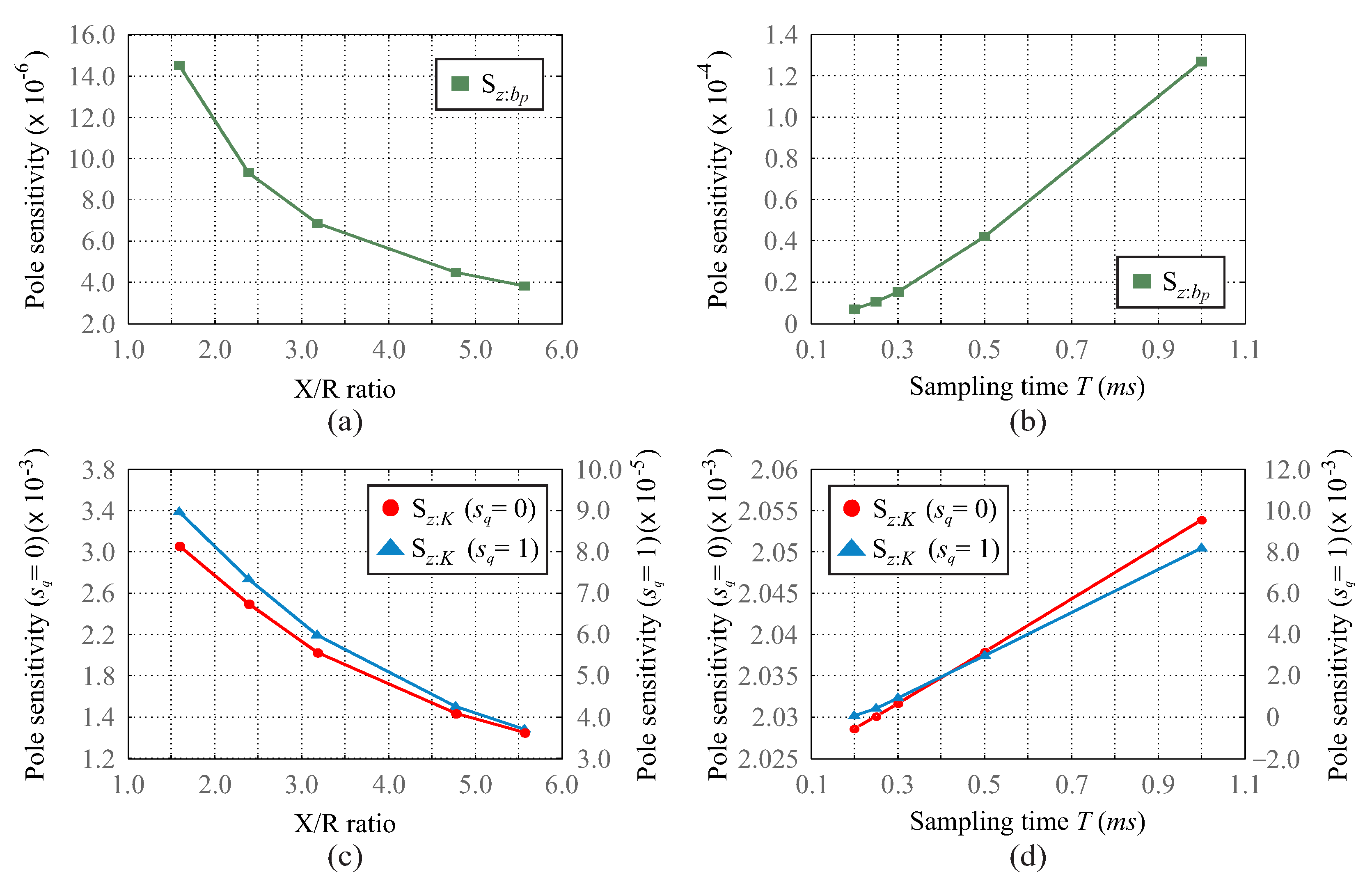
Figure 11 presents the sensitivity of the closed-loop poles for the active and reactive power control under different ratio values and sampling times. According to Figure 11a, when the ratio increases from to , the sensitivity to the parameter decreases from to , which results in closed-loop poles being less sensitive to variations in control gains. Thus, for the system operating with a high value of the ratio, large variations in the control gains cause small displacement in the closed-loop poles. On the other hand, for a low value of the ratio, small variations in can cause large changes in closed-loop poles, making it difficult to adjust the control gain to achieve the desired dynamic response.
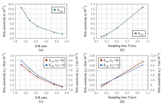
Figure 11.
Sensitivity of the closed-loop poles of the (a) active power control for variations, (b) active power control for T variations, (c) reactive power control for variations, and (d) reactive power control for T variations.
According to Figure 11c, the sensitivity of the closed-loop poles for the reactive power control under different ratio values behaves similarly for both operating modes, i.e., when the ratio increases, the sensitivity to the parameter K decreases. However, for the voltage support mode, the sensitivity values are higher than the case of the reactive power support mode, considering the same value of the ratio. Also, similar to pole sensitivity in the case of active power control, operating with a low value of the ratio can make it difficult to adjust the control gain to achieve the desired dynamic response.
The sampling time also influences the pole sensitivity for the active and reactive power control, as shown in Figure 11b,d. For sampling time values between s and s, the sensitivity value for the active power control increased from to , while for the reactive power control with it increased from to , and with , from to . Thus, for a high value of the sampling time, large variations in the power control gains cause a large displacement in the closed-loop poles.
6. Performance Assessment
To evaluate the effectiveness of the proposed analysis and design method applied to the discrete-time power controllers, the DG system illustrated in Figure 1 is implemented in PSIM. The simulation study is conducted using the system parameters listed in Table 1 and Table 2. The LC filter design for the grid-connected converter follows the methodology presented in [29].
6.1. VSG Controller Performance Analysis
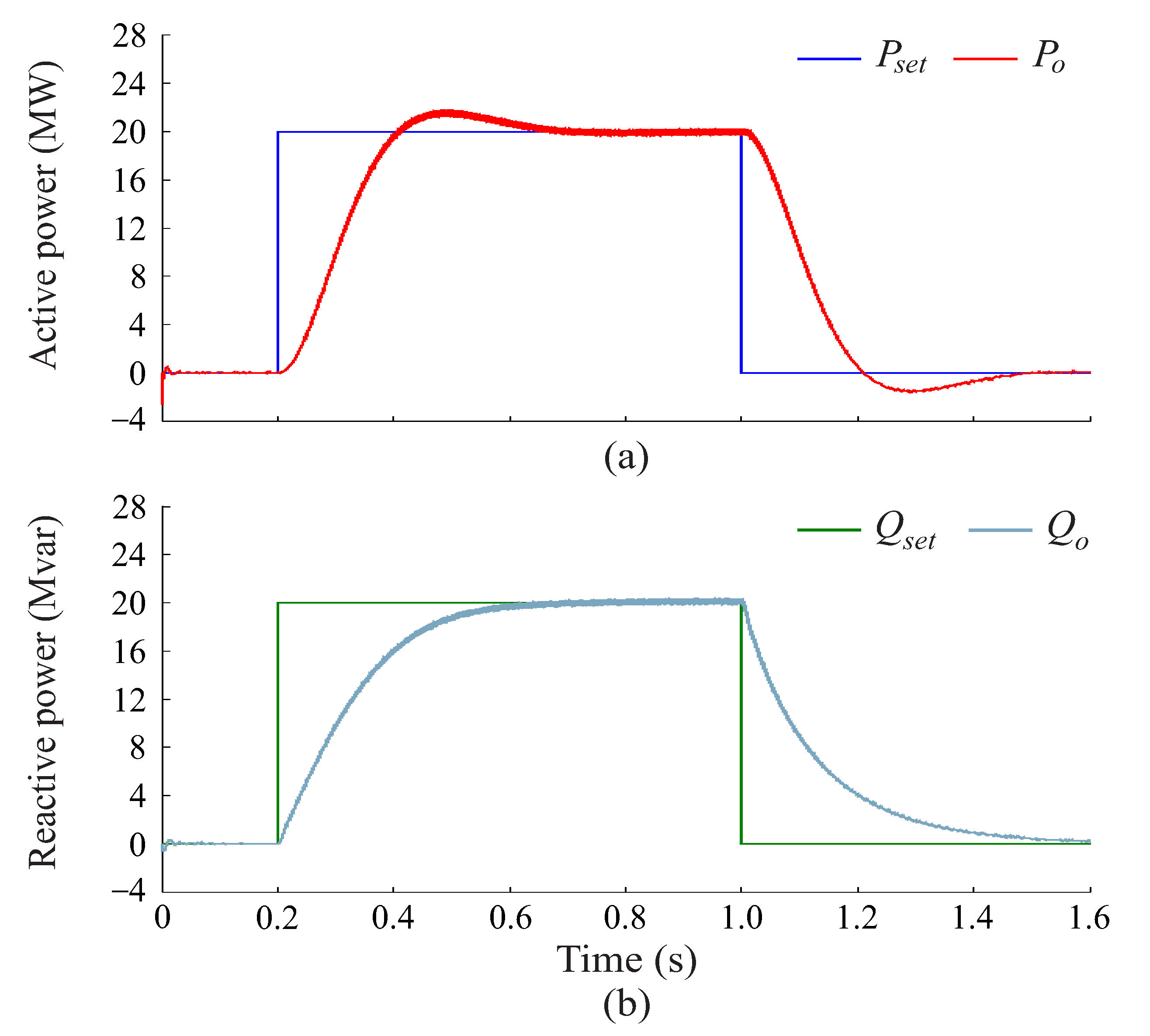
Figure 12 shows the dynamic performance of the active and reactive power controllers in the VSG strategy considering the nominal value of Thevenin equivalent impedance. According to Figure 12a, when a step variation from 0 to 20 MW is applied, the active power converges accurately to the reference value, presenting an overshoot of approximately % and a settling time of about s. Similarly, the reactive power converges accurately to the reference value with a settling time of approximately s during a step variation from 0 to 20 Mvar, as shown in Figure 12b. Therefore, the transient responses of both active and reactive power controllers are consistent with the desired dynamic performance, demonstrating the effectiveness of the dynamic modeling and the design method applied to the discrete-time VSG controllers.
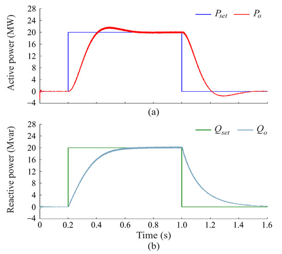
Figure 12.
Controller dynamic performance: (a) active power; (b) reactive power.
6.2. Performance Analysis for Grid Impedance Variation
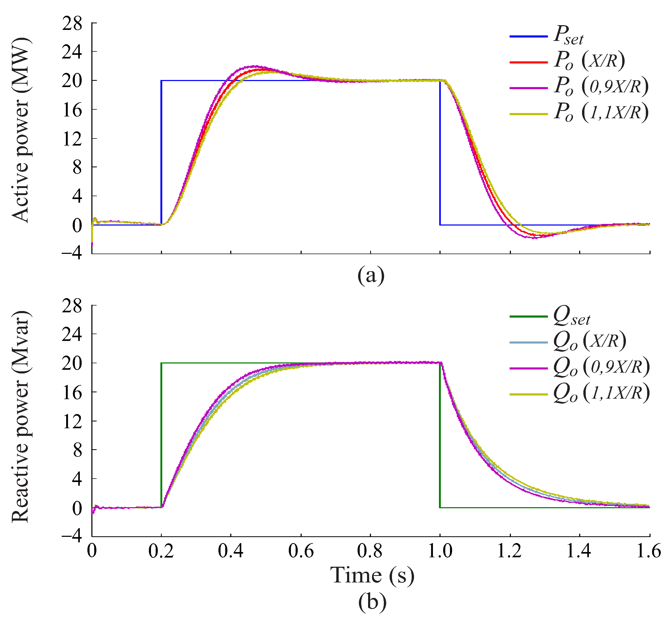
Figure 13, Figure 14 and Figure 15 show the active and reactive power controller responses under the effect of ratio variation. According to Figure 13, a variation in the ratio did not significantly impact the transient response of the active and reactive power controllers, as the settling time remained approximately the same and the active power controller exhibited only a slight variation in overshoot, increasing from approximately to .
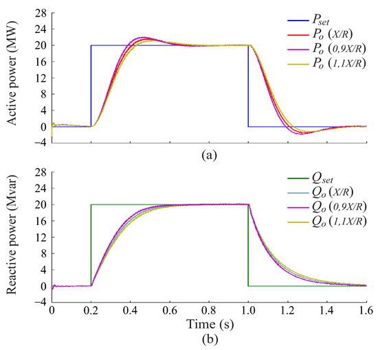
Figure 13.
Power regulation with variation of 10% in the ratio. (a) Active power; (b) reactive power.

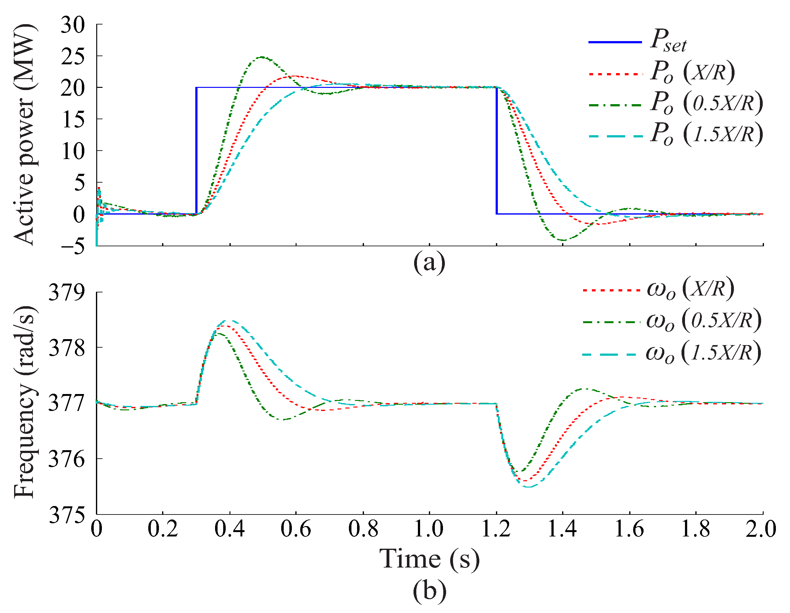
Figure 14.
Active power control with variation of 50% in the ratio. (a) Active power; (b) PCC frequency.
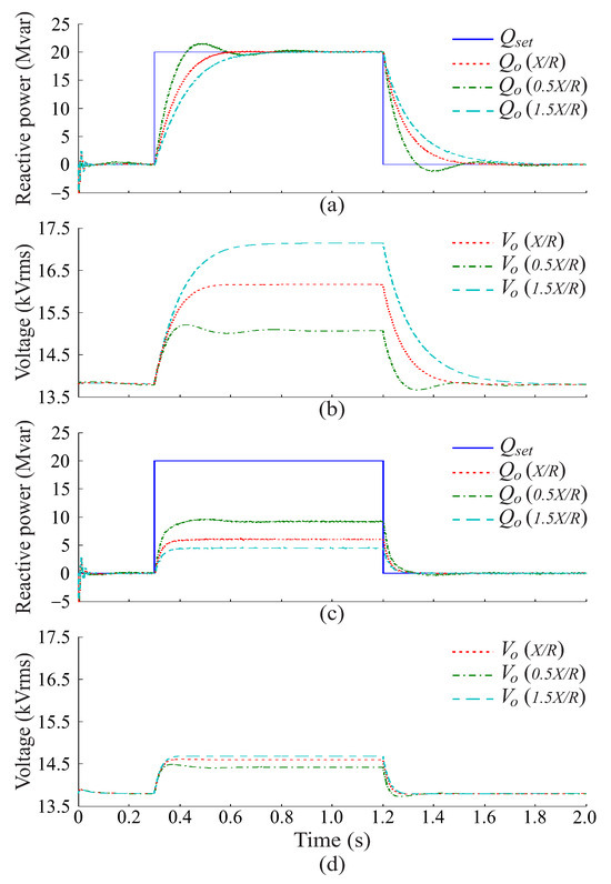
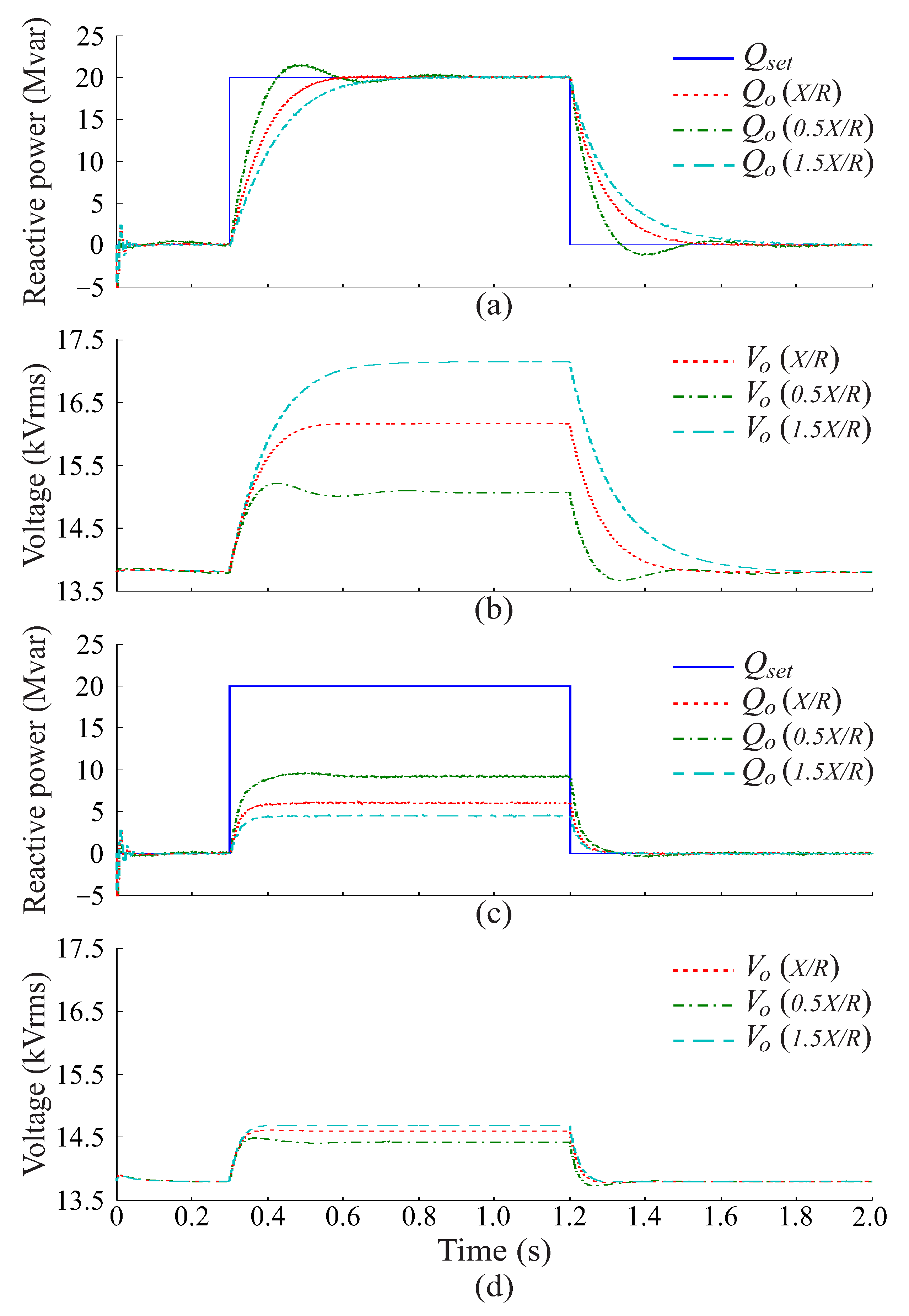
Figure 15.
Reactive power control with variation in ratio. (a) Reactive power (); (b) PCC voltage (); (c) reactive power (); (d) PCC voltage ().
On the other hand, according to Figure 14, variations of 50% in the ratio had a more significant impact on the active power controller response. When the ratio decreased by 50%, the active power controller exhibited a more oscillatory response, with an overshoot of approximately 24%. Conversely, a 50% increase in the ratio resulted in a more damped transient response, without overshoot, as illustrated in Figure 14a. Consequently, variations in the ratio also influenced the PCC frequency behavior of the DG system, as shown in Figure 14b.
Similarly, large variations in the Thevenin impedance also significantly affect the reactive power control of the DG unit. According to Figure 15a, when the VSG scheme operates in reactive power support mode, a 50% decrease in the ratio results in a more oscillatory transient response, with an overshoot of approximately 5%. In this case, the PCC voltage deviates from the system’s nominal voltage, as shown in Figure 15b. On the other hand, when the VSG scheme operates in voltage support mode, the reactive power diverges from its reference value, and a 50% variation in the ratio alters the controller’s steady-state error, as illustrated in Figure 15c. In this case, the deviation between the PCC voltage and the system’s rated voltage is reduced, as shown in Figure 15d.
Table 3 summarizes the desired performance criteria employed in the active and reactive power controller design, along with the corresponding values obtained from their transient response. For comparison purposes, scenarios with 10% and 50% reductions in the nominal grid impedance were listed.
Table 3.
Comparison between design criteria and transient response specifications.
7. Conclusions
This paper presented a dynamic analysis and a design methodology for a discrete-time virtual synchronous generator control strategy applied to a grid-tied distributed generation system. The proposed design approach is based on the root locus method, using a discrete-time model to represent the active and reactive power flow. Controller gains were determined according to predefined dynamic performance criteria, resulting in both active and reactive power controllers exhibiting responses consistent with the desired specifications.
Furthermore, the analysis of the closed-loop poles’ behavior and sensitivity evaluation of the virtual synchronous generator operating in voltage and reactive power support mode highlighted the significant impact of the system’s equivalent impedance and sample time on control performance. The variation in the X/R ratio changed the location of the closed-loop poles within the unit circle, influencing the transient response of the power control. Additionally, the pole sensitivity regarding control gain changed under both impedance variations and different sampling times, emphasizing the need for the analysis using discrete-time modeling. This analysis can provide valuable insights for the tuning of control parameters to improve power flow dynamics. Simulation results validated the theoretical framework and design procedure, demonstrating its effectiveness and practicality for real-world implementation in digital control environments and contributing to enhanced system reliability and stability.
Author Contributions
T.F.d.N. and A.O.S. conceived and designed the study; T.F.d.N. and J.B.O. contributed to data curation, investigation, and methodology; E.R.L.V., J.B.O. and A.O.S. reviewed the manuscript and provided valuable suggestions; T.F.d.N., J.B.O. and E.R.L.V. wrote the paper; and A.O.S. supervised. All authors have read and agreed to the published version of the manuscript.
Funding
This research was funded in part by the Coordenação de Aperfeiçoamento de Pessoal de Nível Superior—Brasil (CAPES)—Finance Code 001 and Conselho Nacional de Desenvolvimento Científico e Tecnológico (CNPq).
Data Availability Statement
Dataset available on request from the authors.
Acknowledgments
The authors would like to thank the CAPES (Coordenação de Aperfeiçoamenteo de Pessoal de Nível Superior) and CNPq (Conselho Nacional de Pesquisa) for the financial support.
Conflicts of Interest
The authors declare no conflicts of interest.
Abbreviations
The following abbreviations are used in this manuscript:
| DG | distributed generation |
| DC | direct current |
| HPWM | hybrid pulse width modulation |
| PCC | point of common coupling |
| RLM | root-locus method |
| RES | renewable energy sources |
| SG | synchronous generator |
| SRF-PLL | synchronous reference frame phase-locked loop |
| VSG | virtual synchronous generator |
| VSC | voltage source converter |
References
- Rocabert, J.; Luna, A.; Blaabjerg, F.; Rodriguez, P. Control of power converters in AC microgrids. IEEE Trans. Power Electron. 2012, 27, 4734–4749. [Google Scholar] [CrossRef]
- Shuai, Z.; Sun, Y.; Shen, Z.J.; Tian, W.; Tu, C.; Li, Y.; Yin, X. Microgrid stability: Classification and a review. Renew. Sustain. Energy Rev. 2016, 58, 167–179. [Google Scholar] [CrossRef]
- Azmy, A.M.; Erlich, I. Impact of distributed generation on the stability of electrical power system. In Proceedings of the IEEE Power Engineering Society General Meeting, San Francisco, CA, USA, 16 June 2005; Volume 2, pp. 1056–1063. [Google Scholar]
- van Wesenbeeck, M.P.N.; de Haan, S.W.H.; Varela, P.; Visscher, K. Grid tied converter with virtual kinetic storage. In Proceedings of the 2009 IEEE Bucharest PowerTech, Bucharest, Romania, 28 June–2 July 2009; pp. 1–7. [Google Scholar]
- Zhu, J.; Booth, C.D.; Adam, G.P.; Roscoe, A.J.; Bright, C.G. Inertia Emulation Control Strategy for VSC-HVDC Transmission Systems. IEEE Trans. Power Syst. 2012, 28, 1277–1287. [Google Scholar] [CrossRef]
- Torres, M.A.; Lopes, L.A.C.; Morán, L.A.; Espinoza, J.R. Self-Tuning Virtual Synchronous Machine: A Control Strategy for Energy Storage Systems to Support Dynamic Frequency Control. IEEE Trans. Energy Convers. 2014, 29, 833–840. [Google Scholar] [CrossRef]
- Zhong, Q.; Nguyen, P.; Ma, Z.; Sheng, W. Self-Synchronized Synchronverters: Inverters Without a Dedicated Synchronization Unit. IEEE Trans. Power Electron. 2014, 29, 617–630. [Google Scholar] [CrossRef]
- Guan, M.; Pan, W.; Zhang, J.; Hao, Q.; Cheng, J.; Zheng, X. Synchronous Generator Emulation Control Strategy for Voltage Source Converter (VSC) Stations. IEEE Trans. Power Syst. 2015, 30, 3093–3101. [Google Scholar] [CrossRef]
- D’Arco, S.; Suul, J.A.; Fosso, O.B. A Virtual Synchronous Machine implementation for distributed control of power converters in SmartGrids. Electr. Power Syst. Res. 2015, 122, 180–197. [Google Scholar] [CrossRef]
- Rodríguez, P.; Citro, C.; Candela, J.I.; Rocabert, J.; Luna, A. Flexible Grid Connection and Islanding of SPC-Based PV Power Converters. IEEE Trans. Ind. Appl. 2018, 54, 2690–2702. [Google Scholar] [CrossRef]
- do Nascimento, T.F.; Salazar, A.O. Improving Transient Response of a Synchronous Generator Emulation Technique Applied to Grid-tied Converters. In Proceedings of the 2021 Brazilian Power Electronics Conference (COBEP), Joao Pessoa, Brazil, 7–10 November 2021; pp. 1–7. [Google Scholar]
- Wang, X.; Li, Y.W.; Blaabjerg, F.; Loh, P.C. Virtual-Impedance-Based Control for Voltage-Source and Current-Source Converters. IEEE Trans. Power Electron. 2015, 30, 7019–7037. [Google Scholar] [CrossRef]
- Du, Y.; Guerrero, J.M.; Chang, L.; Su, J.; Mao, M. Modeling, analysis, and design of a frequency-droop-based virtual synchronous generator for microgrid applications. In Proceedings of the 2013 IEEE ECCE Asia Downunder, Melbourne, VIC, Australia, 3–6 June 2013; pp. 643–649. [Google Scholar]
- Shintai, T.; Miura, Y.; Ise, T. Oscillation Damping of a Distributed Generator Using a Virtual Synchronous Generator. IEEE Trans. Power Deliv. 2014, 29, 668–676. [Google Scholar] [CrossRef]
- Wu, H.; Ruan, X.; Yang, D.; Chen, X.; Zhao, W.; Lv, Z.; Zhong, Q.C. Small-Signal modeling and parameters design for virtual synchronous generators. IEEE Trans. Ind. Electron. 2016, 63, 4292–4303. [Google Scholar] [CrossRef]
- Roldán-Pérez, J.; Rodríguez-Cabero, A.; Prodanovic, M. Design and Analysis of Virtual Synchronous Machines in Inductive and Resistive Weak Grids. IEEE Trans. Energy Convers. 2019, 34, 1818–1828. [Google Scholar] [CrossRef]
- Li, G.; Ma, F.; Wang, Y.; Weng, M.; Chen, Z.; Li, X. Design and Operation Analysis of Virtual Synchronous Compensator. IEEE J. Emerg. Sel. Top. Power Electron. 2020, 8, 3835–3845. [Google Scholar] [CrossRef]
- Chen, M.; Zhou, D.; Wu, C.; Blaabjerg, F. Characteristics of Parallel Inverters Applying Virtual Synchronous Generator Control. IEEE Trans. Smart Grid 2021, 12, 4690–4701. [Google Scholar] [CrossRef]
- Guo, J.; Chen, Y.; Wang, L.; Wu, W.; Wang, X.; Shuai, Z.; Guerrero, J.M. Impedance Analysis and Stabilization of Virtual Synchronous Generators With Different DC-Link Voltage Controllers Under Weak Grid. IEEE Trans. Power Electron. 2021, 36, 11397–11408. [Google Scholar] [CrossRef]
- Nascimento, T.F.d.; Salazar, A.O. Impedance Model Based Dynamic Analysis Applied to VSG-Controlled Converters in AC Microgrids. IEEE Trans. Ind. Appl. 2023, 59, 2720–2730. [Google Scholar] [CrossRef]
- Nise, N.S. Control Systems Engineering, 6th ed.; John Wiley & Sons, Inc.: Hoboken, NJ, USA, 2011. [Google Scholar]
- Nascimento, T.F.D.; Salazar, A.O. Parameters Design of a Digital VSG Control Strategy for Grid-Forming DG Systems Applications. In Proceedings of the 2023 15th IEEE International Conference on Industry Applications (INDUSCON), São Bernardo do Campo, Brazil, 22–24 November 2023; pp. 1588–1593. [Google Scholar]
- Leon, A.E.; Mauricio, J.M. Control strategy to improve damping and transient response of VSG-based renewable power plants. Electr. Power Syst. Res. 2025, 247, 111802. [Google Scholar] [CrossRef]
- Shaikh, M.S.; Raj, S.; Ikram, M.; Khan, W. Parameters estimation of AC transmission line by an improved moth flame optimization method. Electr. Syst. Inf. Technol. 2022, 9, 25. [Google Scholar] [CrossRef]
- Shaikh, M.S.; Raj, S.; Ikram, M.; Latif, S.A.; Mbasso, W.F.; Kamel, S. Optimizing transmission line parameter estimation with hybrid evolutionary techniques. IET Gener. Transm. Distrib. 2024, 18, 1795–1814. [Google Scholar] [CrossRef]
- ANSI C84.1-2020; Electrical Power Systems and Equipment—Voltage Ratings (60 Hz). American National Standards Institute (ANSI): Washington, DC, USA, 2020.
- Akagi, H.; Watanabe, E.; Aredes, M. Instantaneous Power Theory and Applications to Power Conditioning; IEEE Press: Piscataway, NJ, USA, 2007. [Google Scholar]
- Blasko, V. Analysis of a hybrid PWM based on modified space-vector and triangle-comparison methods. IEEE Trans. Ind. Appl. 1997, 33, 756–764. [Google Scholar] [CrossRef]
- Peña-Alzola, R.; Liserre, M.; Blaabjerg, F.; Ordonez, M.; Yang, Y. LCL-Filter Design for Robust Active Damping in Grid-Connected Converters. IEEE Trans. Ind. Inform. 2014, 10, 2192–2203. [Google Scholar] [CrossRef]


Disclaimer/Publisher’s Note: The statements, opinions and data contained in all publications are solely those of the individual author(s) and contributor(s) and not of MDPI and/or the editor(s). MDPI and/or the editor(s) disclaim responsibility for any injury to people or property resulting from any ideas, methods, instructions or products referred to in the content. |
© 2025 by the authors. Licensee MDPI, Basel, Switzerland. This article is an open access article distributed under the terms and conditions of the Creative Commons Attribution (CC BY) license (https://creativecommons.org/licenses/by/4.0/).