Stochastic Demand-Side Management for Residential Off-Grid PV Systems Considering Battery, Fuel Cell, and PEM Electrolyzer Degradation

Abstract

The proposed study incorporates a stochastic demand side management (SDSM) strategy for a self-sufficient residential system powered from a PV source with a hybrid battery–hydrogen storage system to minimize the total degradation costs associated with key components, including Li-io batteries, fuel cells, and PEM electrolyzers. The uncertainty in demand forecasting is addressed through a scenario-based generation to enhance the robustness and accuracy of the proposed method. Then, stochastic optimization was employed to determine the optimal operating schedules for deferable appliances and optimal water heater (WH) settings. The optimization problem was solved using a genetic algorithm (GA), which efficiently explores the solution space to determine the optimal operating schedules and reduce degradation costs. The proposed SDSM technique is validated through MATLAB 2020 simulations, demonstrating its effectiveness in reducing component degradation costs, minimizing load shedding, and reducing excess energy generation while maintaining user comfort. The simulation results indicate that the proposed method achieved total degradation cost reductions of 16.66% and 42.6% for typical summer and winter days, respectively, in addition to a reduction of the levelized cost of energy (LCOE) by about 22.5% compared to the average performance of 10,000 random operation scenarios.

1. Introduction

Ensuring a continuous electricity supply to rural regions poses significant economic challenges, especially in developing countries. Projections indicate that by 2030, approximately 87% of the population in remote areas of developing countries will remain without access to reliable electricity [1]. Utilizing renewable energy resources, such as photovoltaic (PV) and wind systems, offers a viable solution to address the electrification challenges in rural areas. Therefore, the energy system is converted to be decentralized where energy generation from renewable sources is close to load centers [2]. These decentralized energy systems use renewable sources, such as PV, which cannot be dispatched and fluctuate depending on weather conditions. Therefore, energy storage systems are necessary to maintain the supply–demand balance. Li-ion batteries are widely used to tackle the daily imbalance between PV generation and load demand. They store excessive energy when the PV power exceeds load power and discharge when the load is larger than the generated power from PV. There is another load–source imbalance in the seasonal time scale due to higher PV generation in summer than in winter, especially in cold regions. So, a high capacity of PV and storage batteries is required to ensure system reliability, thus increasing both the capital cost and the dumping energy during the summer [3]. Moreover, due to technical and economic constraints, batteries cannot be used for long-term storage. Therefore, a PV system with battery storage is not a valuable solution to tackle seasonal imbalance. Hydrogen is one of the most attractive solutions that provide long-term storage where excessive energy during summer can be converted into hydrogen through an electrolyzer and stored in a hydrogen tank. In winter, a fuel cell converts the stored hydrogen into electricity to supply the load [4,5].

Hydrogen is gaining significant attention because of its high energy density, long-term storage suitability, and environmentally friendly nature. The European Union (EU) aims to reach a 10 million ton hydrogen production rate by 2030 by installing about 40 GW of electrolyzers fed from renewable sources to help decarbonize [3]. In rural areas, hydrogen can also be used for cooking during winter due to the higher efficiency of direct conversion from H2 to heat than conversion of H2 to electricity via fuel cells, then fed to an electric stove. The Wobbe index number for H2 equals about 48 MJ/m³, which does not exceed the safety range for burners according to European standards [6]. However, the flame speed of hydrogen is much higher than natural gas, so it requires careful burner design. The authors of [7] present an experimental study of developing an HHO gas burner with thermal efficiency, reaching about 76% at the maximum flow rate of HHO gas. Several studies are found in the literature that are related to hydrogen cooking based on PV sources, such as the study in [8], which states that PV systems with hydrogen for storage and cooking outperform other systems that use battery storage and propane or induction for cooking, in terms of higher reliability, smaller size, and minimum weight. Also, the authors of [9] propose a novel, safe, and reliable design for hydrogen cooking stoves for self-sufficient houses fed from PV sources. Moreover, the study in [10] suggests a system to produce the required hydrogen for cooking using a PV source. The simulation results show the effectiveness of the proposed model in providing sustainable cooking fuel, but it suffers from significant installation costs. The authors of [11] use social practice theory to illustrate the effect of hydrogen properties on its use as cooking fuel. They also suggest a suitable colorant for hydrogen for use in cooking practices. All these previous studies support using hydrogen for long-term storage and as cooking fuel, particularly in rural areas. However, this currently faces the challenge of high installation costs, but increasing investment and research in hydrogen production and storage will significantly reduce the production cost of fuel cells and electrolyzers in the near future [12,13].

Demand side management (DSM) represents a promising approach to optimizing energy consumption and enhancing system efficiency, particularly for decentralized energy systems. DSM has had a serious concern recently due to the introducing of efficient and smart devices at both residential and commercial levels. DSM can provide various benefits such as increased supply reliability, cost reduction, peak demand reduction, voltage issues mitigation, and emissions reduction [14]. There are many studies in the literature related to residential DSM such as that of [15], which presents a peak shaving technique for DSM to minimize energy consumption cost via optimizing the HVAC power consumption. Still, this study does not consider other appliances that can contribute to DSM, but the study in [16] proposes a direct control method for home appliances to minimize the electricity bill. The authors of [17] present a review of residential DSM; it can be realized that most of these techniques aim to reduce energy costs while achieving user comfort. The authors of [18] present a stochastic dynamic programming approach to optimize energy management of residential loads with electric vehicles to improve load balancing and reduce energy costs. The study of [19] elaborated on the struggles of residential demand response under uncertain consumer behavior and presented an analysis of aggregator decisions to lead to more efficient energy allocation. These studies bring to attention the significance of DSM strategies in balancing energy demand and supply, which can be useful for applications in off-grid systems, specifically when renewable energy sources like PV systems are included. Also, the study of [20] proposed a stochastic energy management strategy for autonomous PV-microgrid systems that seek to capture unpredictable load consumption behavior and improve the stability and efficiency of the system.

Recent studies examining the integration of DSM and hydrogen stores utilize a variety of modeling methods, optimization frameworks, and case studies, contributing considerably to the flexibility and sustainability of the power systems. An array of multi-objective methods has been developed: one hierarchical model furthers the co-planning of hydrogen storage units and vehicle-to-grid services to minimize annualized costs and renewable curtailment [21], and a multi-objective scheduling framework balances the demand fine-tuning and matching needs of peak-load reduction, environmental implications, and total cost through hydrogen-to-power resources and demand shifts [22]. The authors of [23] present a techno-economic study for a case study in Upper Egypt to show how simultaneous hydrogen storage utilization, photovoltaics, and DSM measures can reduce net costs and CO₂ emissions in real-world systems. Other studies use interval and robust optimization to address energy price and renewable generation uncertainty and demonstrate that coupling hydrogen storage with demand flexibility can lead to noteworthy economic results. However, results also highlight the challenges of matching hydrogen conversion efficiencies with evolving consumer demands [24]. These findings underscore the importance of coordinating hydrogen storage operation with DSM to ensure reliability, longevity, and economic efficiency. Furthermore, hybrid strategies using hydrogen and battery storage and real-time control techniques (for example, fuzzy-based demand response and electric vehicle charging) show how load shifting and tuning can improve renewable utilization and reduce dependence on fuel cells [25]. Therefore, co-optimizing hydrogen storage, DSM, and hybrid strategies is crucial to meeting reliability, economic, and environmental goals but exposes new obstacles, including response fatigue, the complexity of system-level operation, and the necessity of improved predictions, to which future investigations must be addressed. Furthermore, it is important to coordinate hydrogen storage operation with DSM to mitigate system component degradation, ensuring extended service life and cost-effectiveness.

In hybrid battery–hydrogen storage systems, frequent charging and discharging cycles of batteries, electrolyzers, and fuel cells lead to significant degradation of these components over time. This degradation process reduces component lifespan and increases capital costs, which pose an economic barrier to the development of such systems. The degradation process of Li-ion batteries, fuel cells, and electrolyzers has been illustrated in the literature in detail. Some previous studies assumed a fixed Li-ion battery lifespan and neglected the degradation [26]. However, this is not valid and may cause multiple battery replacements. Other studies limit the daily battery cycles to increase their lifetime, affecting the operation flexibility [27]. The authors of [28] propose a Li-ion battery cycle aging model that can be easily incorporated in dispatch programs. Moreover, fuel cell and PEM electrolyzer degradation processes have been studied in some studies, such as in [29,30], that model the aging process due to the operating conditions. The operation of these components must be managed in such a way that their degradation process is reduced. DSM represents a promising approach to mitigating system degradation by optimizing and reshaping the consumption patterns on the end-user side. To the best of our knowledge, no previous studies have implemented DSM in an off-grid PV system fed residential load to minimize the degradation cost.

The current study proposes a stochastic DSM (SDSM) strategy to minimize the total degradation cost of the battery, fuel cell, and PEM electrolyzer for the considered system that uses PV as a primary source and the storage system is a hybrid Li-ion battery with hydrogen to balance daily and seasonal load–source imbalance. This system feeds a residential house in rural areas with the required energy for electrical appliances and cooking. Uncertainty of house demand prediction is incorporated using the scenario generation method to enhance the accuracy and robustness of the proposed technique. Then, the stochastic optimization problem is solved using the genetic algorithm (GA) to determine the optimal schedules of deferable appliances and the optimal settings of a water heater (WH).

The main contribution of the proposed study focuses on developing SDSM for isolated PV systems that feed single residential houses in rural areas and use hybrid Li-ion batteries with hydrogen storage to minimize the total degradation cost and enhance consumer welfare. The key contributions of the proposed study are summarized as follows:

• This study proposes an innovative SDSM strategy for off-grid PV systems with hybrid Li-ion battery–hydrogen storage that significantly minimizes the degradation of principal components and reduces the levelized cost of energy (LCOE).
• The uncertainty of load predictions is incorporated into the optimization problem using scenario-based generation to enhance the accuracy and robustness of the proposed approach.
• Simulation results validate the economic and operational benefits of the proposed SDSM method, achieving up to a 22.5% reduction in LCOE, zero load shedding, and minimal energy dumping compared to random operation scenarios.

The remainder of the paper is organized as follows. Section 2 describes the proposed SDSM methodology in detail. Section 3 discusses simulation results and discussion. Finally, Section 4 concludes the paper.

2. Methodology

As shown in Figure 1, the proposed system is a self-sufficient house fed from a PV panel with a hybrid battery–hydrogen storage system. Moreover, hydrogen and HHO gases are used as fuel for cooking. In the summer daytime, the HHO electrolyzer is used to convert electrical energy into HHO gas, which is used directly for cooking. In winter days and times of insufficient irradiation, H2 gas is used directly for cooking because this is more efficient than converting hydrogen to electricity via fuel cells to supply induction cooking. Since the system is off grid, the proposed SDSM strategy aims to minimize the operation cost, represented by the total degradation cost of the battery, PEM electrolyzer, and fuel cell. Accurate prediction of the house power consumption is essential for making efficient DSM. However, single-house load prediction is challenging since it depends on consumer behavior, which causes high uncertainty in demand forecasting. The proposed study uses a scenario-based generation technique for electrical and cooking power consumption to account for this uncertainty. The following sections describe the modeling of uncertainty in load prediction, the degradation model of different components, and the proposed SDSM strategy for a single self-sufficient house supplied from a PV source.

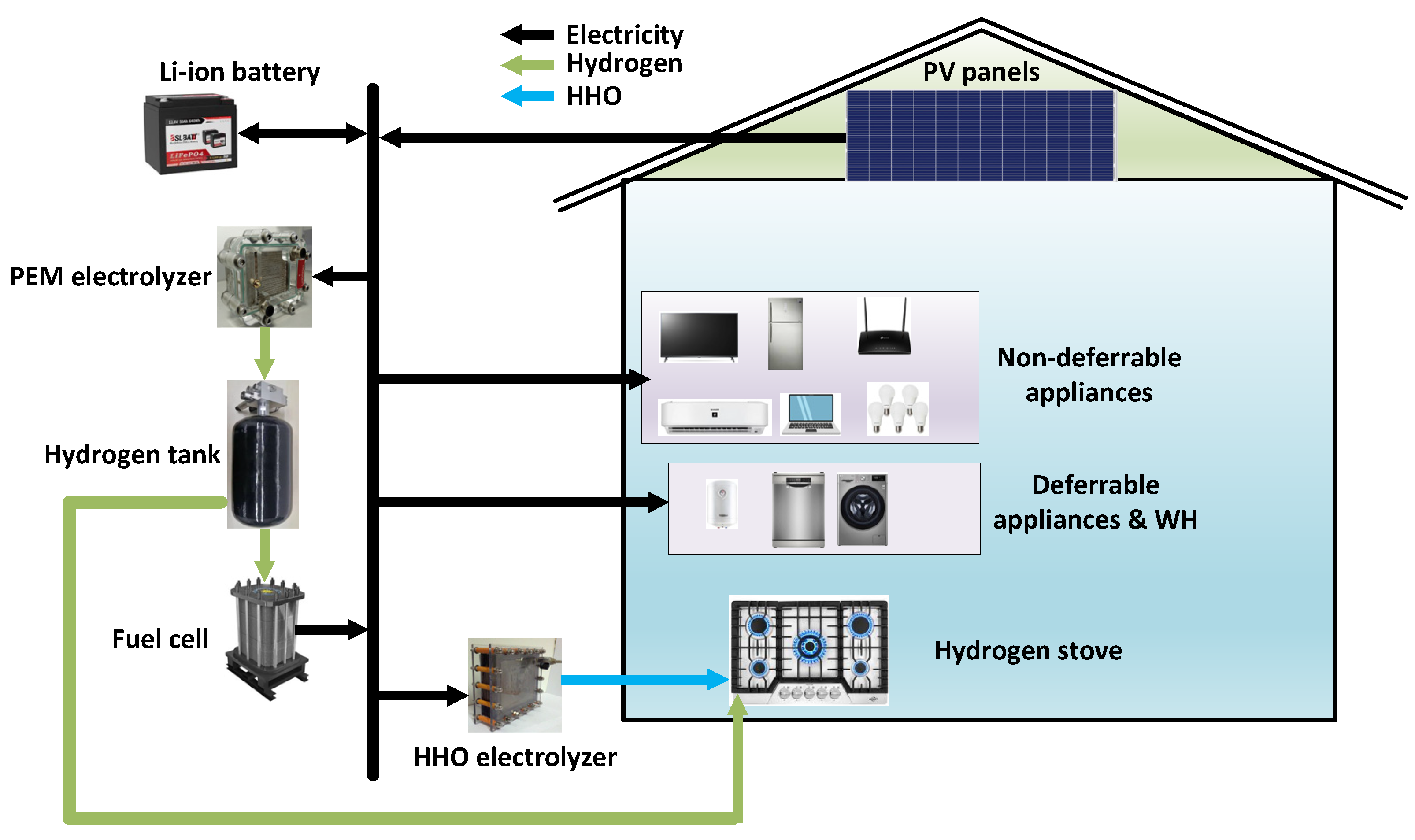
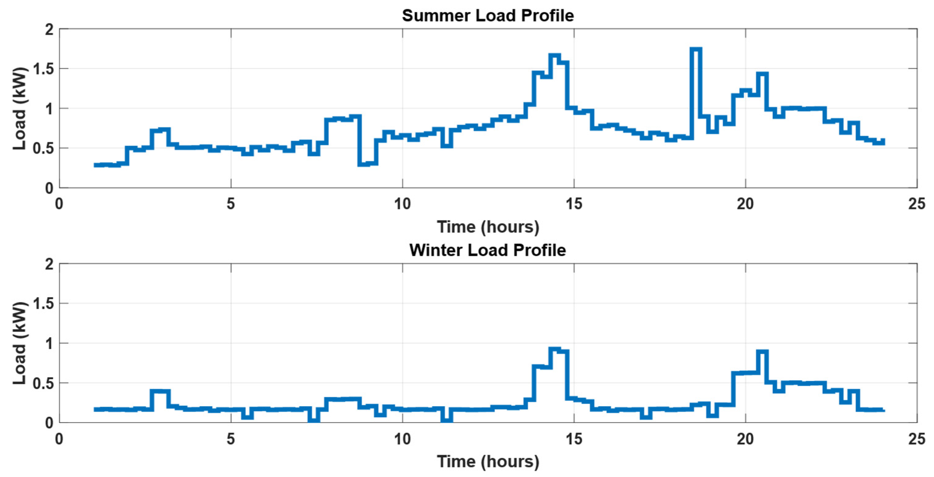
2.1. Typical Electrical Load Profile and Appliance Classification

The ability of home appliances to participate in SDSM varies significantly based on their manageability. Existing literature classifies home appliances into three distinct categories, as found in [17]. In the proposed study, home appliances are classified into three categories as follows:

• Non-deferable loads: These loads cannot participate in SDSM programs due to their non-deferable nature. Examples of loads in this category are lights, fans, personal laptops, televisions, refrigerators, and routers.
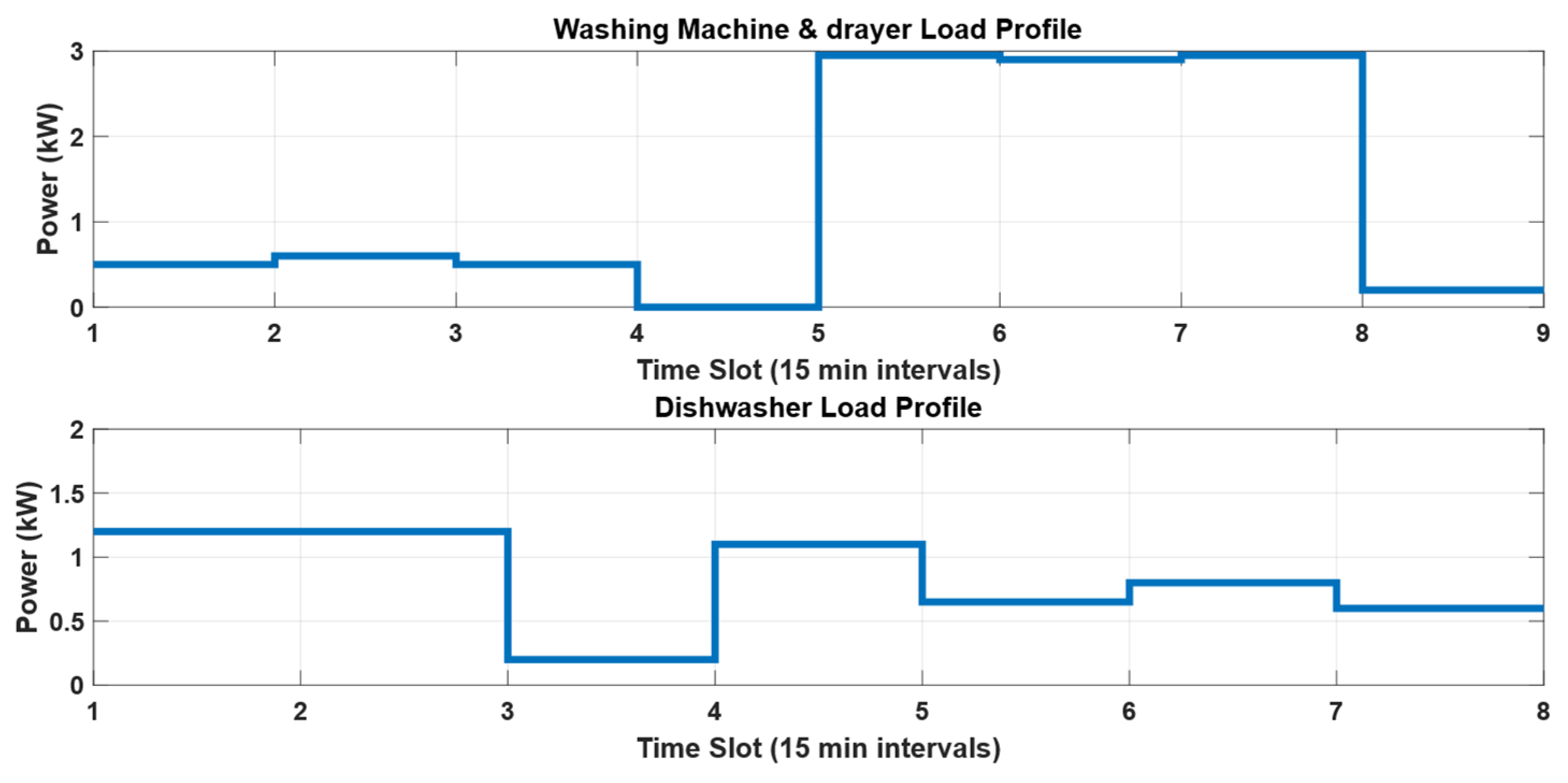
• Deferable loads: The operation of these loads can be scheduled within a predefined time window set by the customer. Once initiated, these loads cannot be interrupted, and they must complete their full operating cycle. Examples of loads in this category include appliances such as washing machine and dryer (WM) and dishwasher (DW).
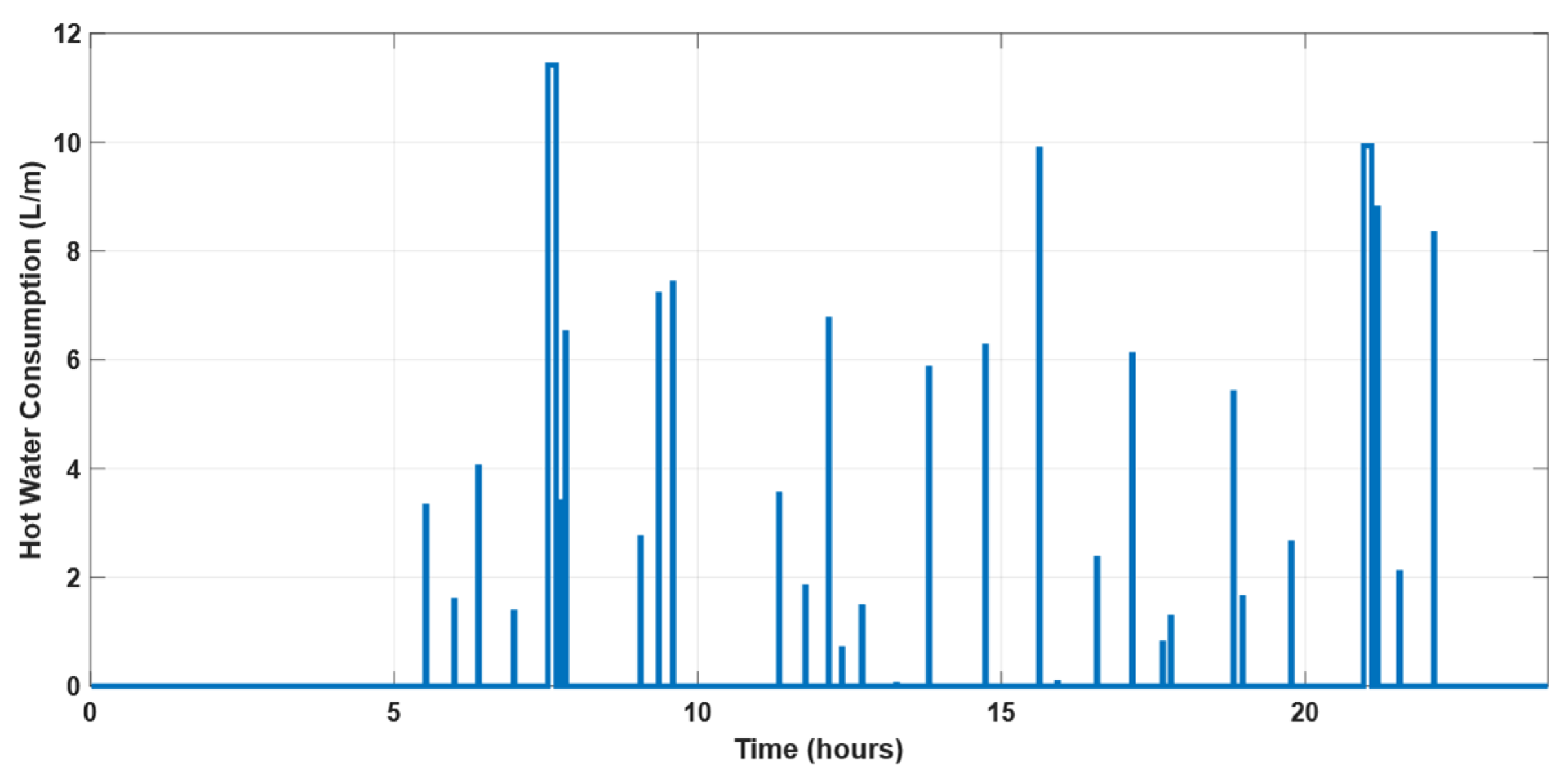
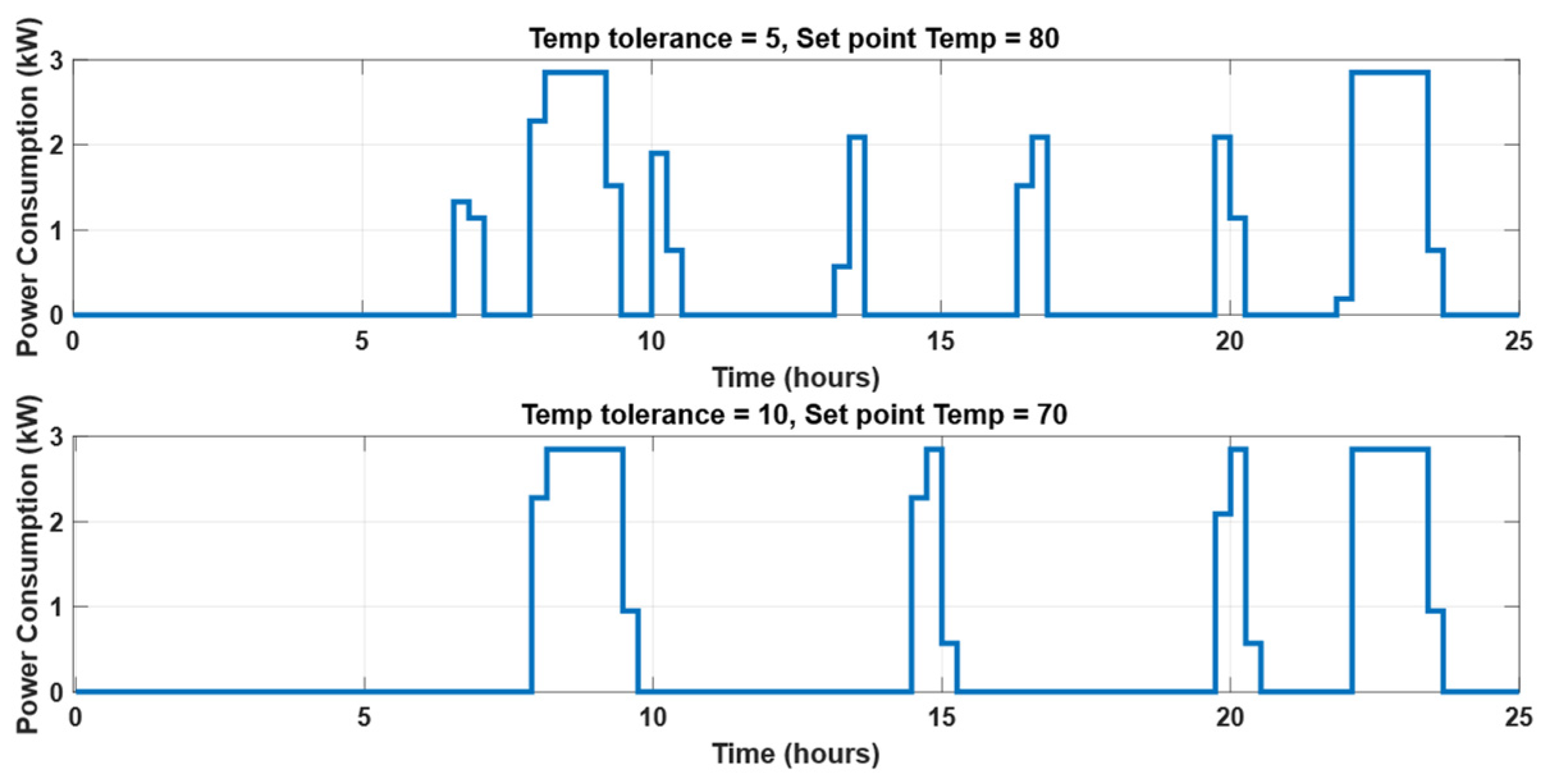
• Thermostatically controlled: These loads can contribute to SDSM due to their thermal capacity and inertia, so their power consumption profile can be controlled without affecting user comfort level. WH is an example of this load category.

The following discussion provides the characteristics of the appliance consumption profile in each category.

• Load profile of non-deferable loads

In this study, the consumption activity of different appliances of non-deferable loads in a typical single-family house is illustrated in

Table 1. Non-deferable appliance rating and operating times for a typical single-family house.

Appliance Name	Rating (W)	Quantity	Operating Time (h)
Refrigerator	140	1	00:00 to 23:59
Router	10	1	00:00 to 23:59
Lights (LED)	15	1	00:00 to 23:59
	12	2	07:00 to 09:00
			12:00 to 14:00
			18:00 to 20:00
	15	2	18:00 to 23:00
TV	100	1	07:00 to 08:00
			13:00 to 15:00
			20:00 to 22:00
Personal computer	200	1	20:00 to 23:00
Fans (summer only)	100	2	00:00 to 09:00
			12:00 to 23:59
Inverter air conditioner (summer only)	1500	2	Table 2
Others	400	1	2 h ~ Uniform [07:00 to 23:59]

. Figure 2 shows the electrical load profiles for this house on typical summer and winter days, considering only the non-deferable loads. The consumption profiles for various appliances were derived from real datasets utilized in the referenced study [31], ensuring the incorporation of realistic and accurate energy usage patterns.

The current study used the inverter air conditioner model presented in the study [32]. Its consumption power is represented by discrete values, dependent on the difference between the set point temperature and the measured temperature of the room. When the temperature difference is significant, the power consumption is set to the rated value, and as the temperature difference decreases, the power consumption reduces accordingly. Therefore, the following equation provides the consumption power for inverter air conditioners.

$$P_t^{HVAC}=\left[0.2 {\delta }_t^1+0.4 {\delta }_t^2+0.6 {\delta }_t^3+0.8 {\delta }_t^4+{\delta }_t^5\right]P^{HVAC}$$

(1)

where ${\delta }_t^i$ is a set of binary decision variables, with only one binary variable equal to one at a time and others set to zero. The room temperature at time slot t ($T_t^{in})$ is given by the following equation:

$$T_t^{in}=\alpha T_{t-1}^{in}+\beta T_{t-1}^{out}-\gamma P_t^{HVAC}$$

(2)

where $T_{t-1}^{out}$ is the output temperature, and the technical parameters of the inverter air conditioner $\alpha$, $\beta$, and $\gamma$ are given in

Table 2. Technical parameters of the inverter air conditioner system [32].

${\mathit{P}}^{\mathit{H}\mathit{V}\mathit{A}\mathit{C}}$(kW)	$\alpha$	$\beta$	$\gamma$ (°C/kW)	Temperature Set Point
1.5	0.99	0.01	0.29	24 °C for t ϵ {[0:00–8:00] U [18:00–0:00]}
				26 °C for t ϵ {[8:00–18:00]}

.

2.

Load profile of deferable loads

DW and WM are classified as deferable loads, with their load profiles influenced by technical specifications and operating modes. As a result, each household exhibits distinct patterns for the power consumption profile of these appliances. In this study, the load profiles of these devices are derived from a real measurement dataset [31]. As shown in Figure 3, the DW profile has three sub-cycles: wash, rinse, and dry. A complete cycle takes roughly 105 min, and the power consumption varies from 1.2 kW to 0.6 kW. For a WM and dryer, as shown in Figure 3, the WM operates for about 45 min, comprising three sub cycles: wash, rinse, and spin, with power consumption ranging from 0.52 kW to 0.65 kW. After a 15 min delay, the dryer initiates operation and continues for one hour, with power consumption varying between 2.97 kW and 0.19 kW. The proposed strategy aims to find the optimal schedules of those deferable appliances to reshape the overall power consumption profile in such a way that minimizes the degradation process of system components as much as possible.

3.

Load profile of water heater

WH also contributes to SDSM due to its high thermal inertia. The proposed strategy aims to determine optimal temperature tolerance and set point temperature to minimize the objective function and achieve user comfort, i.e., the requirement of hot water consumption. Firstly, WH parameters must be determined, including tank size, heat resistance, and power rate. The WH operation is based on the water temperature in the tank, the temperature set point, and the temperature tolerance. When the water temperature in the tank drops below the lower bound, the water heater starts operating at its rated power. It continues operation until the temperature reaches the upper bound. Therefore, the power consumption by the water heater at each time step i is calculated from the following equation:

$$p_{WH, i}=\left\{\begin{array}{c}{\eta }_{WH }{P}_{WH} T_{tank, i}<T_{set}-tol\\ 0 T_{tank, i}>T_{set}\\ p_{WH, i-1} T_{set}-tol\le T_{tank, i}\le T_{set}\end{array}\right.$$

(3)

where $P_{WH}$ (kW) is the rated power of WH, ${\eta }_{WH }$ (%) is the WH efficiency, $T_{tank, i}$(°F) is the temperature of water in the tank at time slot I, $T_{set}$ (°F) is the set point temperature, and $tol$ (°F) is the lower temperature tolerance. The water tank temperature is calculated from the following equation [33]:

$$T_{tank, i+1}={\displaystyle \frac{T_{tank, i}\left(V_{tank}-HW{D}_i \Delta t\right)}{V_{tank}}}+{\displaystyle \frac{T_{in}HW{D}_i\Delta t}{V_{tank}}}+{\displaystyle \frac{\Delta t}{8.34\ast 60 V_{tank}}}\left[3412 p_{WH, i}-{\displaystyle \frac{A_{tank}\left(T_{tank, i}-T_a\right)}{R_{tank}}}\right]$$

(4)

where $T_{in}$ (°F) is the inlet water temperature, $T_a$ (°F) is the room temperature, $HW{D}_i$ (gallons/m) is the hot water demand flow rate, $A_{tank}$($f{t}^2)$ is the tank surface area, $V_{tank}$ (gallons) is the tank volume, $R_{tank}$ (°F. $f{t}^2.h/Btu)$ is the tank heat resistance, and $\Delta t$ (m) is the time slot duration. The technical specifications of the water heater are given in

Table 3. Technical specification of WH.

${\mathit{P}}_{\mathit{W}\mathit{H}}$ (kW)	${\eta }_{\mathit{W}\mathit{H} }$ (%)	${\mathit{T}}_{\mathit{i}\mathit{n}, °\mathbf{C}}$ (°C)	${\mathit{A}}_{\mathit{t}\mathit{a}\mathit{n}\mathit{k}}$	${\mathit{V}}_{\mathit{t}\mathit{a}\mathit{n}\mathit{k}}$ (gallon)	${\mathit{R}}_{\mathit{t}\mathit{a}\mathit{n}\mathit{k}}$ $(\text{°}\mathbf{F}.\mathit{f}{\mathit{t}}^2.\mathit{h}/\mathit{B}\mathit{t}\mathit{u})$
			$\left(\mathit{f}{\mathit{t}}^2\right)$
3	95	14	22.29	26.45	15

. The operation of the water heater depends on the hot water demand (HWD) consumption profile for the specific household. The current study used the methodology described in [34] as a baseline to establish the HWD consumption profile. This approach measures the HWD consumption patterns and applies a stochastic strategy to generate 1 min profiles of HWD. The probability of both flow rate and time of occurrence depends on the hot water consumption category, as presented in

Table 4. Reference conditions for hot water consumption profile at 45 °C of one family house [34].

Categories	Cat A	Cat B	Cat C [Shower]
Flow rate (L/m)	1	6	8
Duration (m)	1	1	5
Inc/day	28	12	2
σ	2	2	2

. Figure 4 shows the 1 min HWD consumption profile in (L/m) at 45 °C for an example day in the winter for a single-family house. The hot water in the tank is mixed with the incoming mains water to achieve the required HWD temperature of 45 °C. The hot water demand from the water tank, measured in (gallons/m), can be calculated using the following equation:

$$HW{D}_i=HW{D}_{45 °\mathrm{C}, i }{\displaystyle \frac{45-T_{in, °\mathrm{C}}}{T_{tank, i,°\mathrm{C} }-T_{in, °\mathrm{C}}}}$$

(5)

where $HW{D}_{45 °\mathrm{C}, i}$ (gallons/m) is the flow rate at 45 $°\mathrm{C}$ obtained by multiplying the flow rate in Figure 4 by a factor of 0.26417. $T_{in, °\mathrm{C}}$ ($°\mathrm{C}$) and $T_{tank, i,°\mathrm{C} }$($°\mathrm{C}$) are the inlet temperature and tank temperature, respectively. The effect of temperature tolerance and setpoint temperature on the power consumption profile of WH is shown in Figure 5. Therefore, controlling these parameters for WH can contribute to SDSM by reshaping the consumption profile in such a way that reduces degradation cost as much as possible.

2.2. Energy Consumption Profiling for Cooking Using an HHO Stove

In general, the uncertainty of the consumption power profile for cooking comes from different factors, including starting time of preparation, dish type, dish amount, cooking time, and cooking behavior. There are fewer examples in literature for modeling of consumption power profile for cooking, such as the study in [35], where the authors propose a novel strategy to model high-resolution cooking power consumption using the LoadProGen algorithm, which functions as an outer stage. The timing of each cooking cycle and its corresponding power consumption can be adjusted to account for uncertainty. The proposed strategy uses the technique that is described in [35] as a baseline to generate the cooking consumption profiles. There are usually some familiar dishes for each meal in a distinct house, and the cooking habits, such as the starting preparation time and the cooking intervals, tend to fall within a specific range. The main meals in Egypt derived from direct field observations are divided as follows: breakfast typically consists of ful medames, taameya (falafel), bread with cheese or eggs, and tea or milk. Lunch includes some main dishes such as rice, meat or chicken, remaining food, vegetables, chicken pane, traditional dishes, and molokhia. Dinner usually features popular dishes, cheese, vegetables, and fruits, accompanied by tea or coffee. This study aims to model the power consumption profile for cooking lunch only because the stove will feed directly from the HHO electrolyzer during lunch preparation during the summer session, but the preparation of other meals uses H2 gas stored in the tank due to insufficient irradiation so that it does not require to obtain their consumption profile.

Table 5. Detailed data for power consumption during cooking preparation of some familiar lunch dishes in Egypt.

	Dish	Power Range	Average Time Range (Minute)	Average Starting Time Range
1	Rice	Boil: HP	15	01:00 PM to 02:00 PM
		Simmer: LP	20
		Steam: very low power	10
	Meat	Boil: HP	40
		Simmer: LP	65
2	Rice	Boil: HP	15
		Simmer: LP	20
		Steam: very low power	10
	Chicken	Boil: HP	40
		Simmer: LP	50
		Frying: MP	20
3	Molokhia	MP	35
4	Chicken pane	MP	40
5	Vegetables	Boil: HP	25
		Simmer: LP	40
6	Remaining food or fast food	MP	40
7	Delivery or non-cook food	No power	-

illustrates the power ranges, average preparation time, and the range of starting times for preparing different lunch meals. Moreover, the HHO stove, with a total efficiency of 60%, is assumed to have three burners having the power ranges: low-power (LP) (500–1000 W), medium-power (MP) (1100–1500 W), and high-power (HP) (1600–2000 W) [35]. The average starting time of lunch preparation is represented by five instants starting from 01:00 PM to 02:00 PM with 15 min time slots. So, there are 35 scenarios for lunch consumption power profiles with equal probabilities. Similar consumption profiles are merged and represented by one profile with their summing probabilities to reduce the number of scenarios. Figure 6 shows the decreasing scenarios for power consumption of the HHO electrolyzer that feeds the stove during lunch cooking according to the data in Table 5.

2.3. Stochastic Model Description

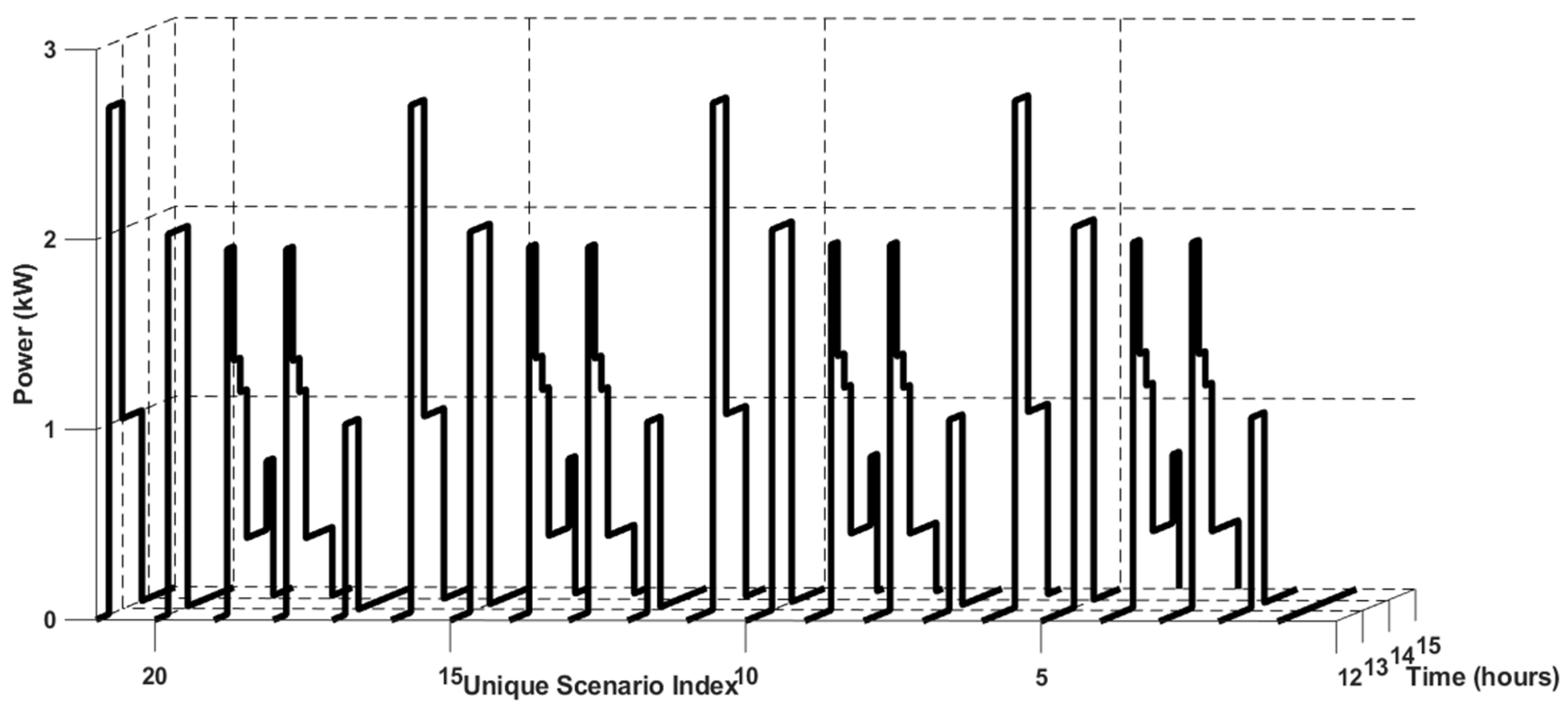
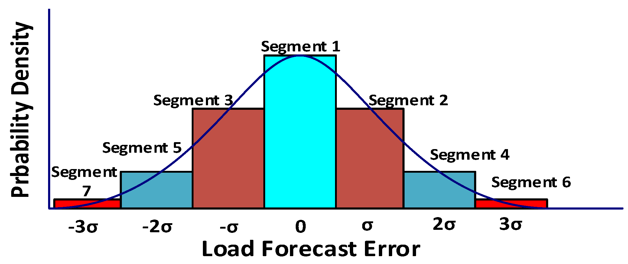
The load profile of non-deferable loads must be predicted with sufficient accuracy to make the SDSM more effective. However, the prediction of the electric consumption power of single houses is challenging due to its dependence on customer behavior, which results in high uncertainty in the predicted power consumption profile. There are different techniques to account for this uncertainty, such as probabilistic load forecasting and scenario-based prediction. The current study used scenario-based generation to model the uncertainty in load forecasting, as illustrated in the following discussion.

• Scenario generation

The proposed scenario generation technique uses a distinct random value within the range [0, 1] that is generated independently using the Sobol sequence for each input random variable. Sobol sequence is superior to the ordinary random number generation method in accuracy and convergence due to its ability to generate low-discrepancy sequences in multi-dimensional spaces [36]. Load prediction uncertainty is modeled based on its error obtained from the probability distribution function (PDF). For instance, typical continuous and discrete forms of PDF for the load prediction at time instant t are shown in Figure 7. A finite set of scenarios can represent the probability of distribution of a load demand forecast. Each scenario corresponds to one specific outcome of the random variables during the study horizon. Moreover, each scenario has a probability that reflects the likelihood of its occurrence. Thus, the following equation can obtain load demand for each scenario [37]:

$$P_{t,s}=P_t^{predicted}+\Delta P_{t,s}t=1,\dots ,96; s=1,\dots ,N_s$$

(6)

where $P_{t,s}$ (kW) is the load value at time t and scenario s, $P_t^{predicted}$ (kW) is the predicted load value at time t, and $\Delta P_{t,s}$ (kW) is the load forecast error at time t and scenario s. The proposed scenario generation technique can be summarized as follows.

Firstly, the PDF function is divided into seven segments; each segment $l$ has a wide equal to the standard deviation error (σ). Moreover, each segment has its probability denoted by ${\beta }_l$. Roulette wheel mechanism (RWM) generates the scenarios at each time slot [37]. In this regard, the accumulative normalized probabilities are obtained for all segments, as shown in Figure 8. Then, a random number is generated between 0 and 1 for each time slot that follows a Sobol sequence. The first segment with an accumulated normalized probability less than or equal to this random number is selected. The load forecast error and the probability of this selected segment are used for this time slot. This process continues until the required number of scenarios is obtained. Moreover, the probability of each scenario can be determined as follows:

$${\pi }_s=\frac{{\prod }_{t=1}^{96}{p}_{t,s}}{{\sum }_{s=1}^{N_S}{\prod }_{t=1}^{96}{p}_{t,s}}$$

(7)

where $p_{t,s}$ is the probability of load prediction for scenario s at time t.

2.

Scenario reduction and stooping rule

The large number of scenarios causes better uncertainty modeling while increasing the computation complexity. Therefore, scenario-reduction techniques are essential to balance the accuracy of the stochastic model and computation complexity. The simultaneous backward technique is used to minimize the number of scenarios [38]. Let ${\mathrm{N}}_s$ denote the total number of scenarios, each characterized by a unique probability ${\pi }_s$, representing the probability of occurrence for the respective scenario. For each scenario s, find the closest scenario with a minimum distance from other scenarios. Next, compute the product of the probability and the minimum distance for each scenario, then select the scenario with the most minor product. Finally, remove this scenario from the set and update the probabilities. These steps are repeated until the desired number of scenarios are achieved. The stopping criteria illustrated in [37] is used in the proposed study by dividing results into batches of scenarios. The stopping rule is applied after each batch, based on the coefficient of variation cv. The simulation ends when the value of cv is below a predefined threshold. The value of cv is calculated based on the following equation.

$$c{v}_r={\displaystyle \frac{{\sigma }_r}{{\mu }_r\sqrt{N_s}}}$$

(8)

where ${\sigma }_r$ is the standard deviation of random variable r, and ${\mu }_r$ is its mean value.

3.

Combination of cooking and electrical load scenarios

During summer, cooking consumption power profiles represent a part of the total electrical load demand so the $N_c$ scenarios of cooking consumption must be combined with $N_e$ non-deferable electrical load profile scenarios. The combined electrical load profile scenarios and their probabilities are given by

$$P_{total,t}^S=L_{electrical,t}^i+L_{cooking,t}^j$$

(9)

where $i=1:N_e$, $i=1:N_c$, and $S$ =$N_e$ $N_c$.

Furthermore, the probability of each scenario within the combined electrical load profile is determined by the product of the probabilities of the corresponding cooking consumption scenario and the non-deferrable electrical load profile scenario that were aggregated to form the combined scenario.

2.4. Sizing of the Proposed System

The size of PV panels must be determined to generate the required annual energy for the house. Moreover, batteries are used for short-term storage, while hydrogen is used for long-term storage. Surplus energy during summer times is converted via a PEM electrolyzer into hydrogen and stored in a tank to be used again in winter sessions to supply loads via fuel cells in addition to its use as a cooking fuel. The current study used the methodology of sizing isolated PV systems with hybrid hydrogen–battery storage, explained in detail in [3]. The key parameter of this sizing technique is the load sizing factor $S{F}_L$ that equals the energy supplied by hydrogen divided by the total consumption energy in the winter session.

$$S{F}_L={\displaystyle \frac{E_{winter, H2}}{E_{winter, total}}}$$

(10)

The range of load sizing factors is between 0 and 1, which determines the system ability to be self-sufficient, but high values of load sizing factors cause high installation cost. Moreover, the load sizing factor for a specific system depends on the yearly load and irradiation profiles. The typical load profiles in Figure 2, deferable load profiles in Figure 3 and Figure 5, in addition to the average daily cooking consumption energy of 6 kWh/day, are used to calculate the average daily consumption energy during winter and summer sessions that are found to be equal 29 kWh/day and 34 kWh/day, respectively. According to [39], the average summer and winter peak sun hours in the chosen location equal 6 and 4 h, respectively. Therefore, the sizing factor can be determined from the following equation:

$$S{F}_L={\displaystyle \frac{1.1 E_{ winter}- P{V}_{rated} S{H}_{winter }day{s}_{winter }}{1.1 E_{ winter}}}$$

(11)

where $E_{ winter}$(kWh) is the average consumption of energy during the winter session, $P{V}_{rated}$ (kW) is the rated power of the PV supply and $S{H}_{winter}$ (hours) is the average peak sun hours in winter at the house location. Factor 1.1 is used to account for all system losses. The PV sizing must be determined to supply the total annual energy of the system and is given by the following equation [3]:

$$E_{pv, total}=1.1 (E_{summer}+\left(1-S{F}_L\right)E_{ winter}+{\displaystyle \frac{S{F}_L E_{ winter}}{{\eta }_{EL} {\eta }_{FC}}}$$

(12)

where $E_{summer}$ (kWh) is the average consumption of energy during the summer session, ${\eta }_{EL}$ (kg/kWh) is the electrolyzer efficiency, and ${\eta }_{FC}$ (kWh/kg) is the fuel cell efficiency. Then, the required rate of PV panels is obtained using the following equation:

$$P{V}_{rated}={\displaystyle \frac{E_{pv, total}}{1000\times SH\times 365}}$$

(13)

where SH (hours) is the average yearly peak sun hours in the desired location. The battery size is designed to supply only one autonomy day, instead of three to five days, because of the inclusion of another storage in form of hydrogen. Thus, the size of the battery is given by

$$E_{battery}={\displaystyle \frac{1.1 E_{average, day}}{DO{D}_{max}}}$$

(14)

where $E_{average, day}$(kWh) is the average daily consumption of energy and $DO{D}_{max}$ (%) is the maximum depth of discharge of the battery.

The fuel cell rate must be chosen to equal the maximum load power throughout the year to ensure zero load shedding, but this will increase the cost. Therefore, the fuel cell rate is chosen to equal only a percentage of the maximum load $L_{cr}$ (%) depending on the user requirements and representing a tradeoff between cost and welfare.

$$P_{FC,rated}=L_{cr} P_{max,year}$$

(15)

The electrolyzer size is chosen to absorb an amount of energy during the summer session and store it in a hydrogen tank to be used in the winter session. The following equation was used to determine the electrolyzer size.

$$P_{EL, rated}={\displaystyle \frac{1.1 S{F}_L E_{ winter}}{{\eta }_{EL} {\eta }_{FC} SH Day{s}_{ summer}}}$$

(16)

The size of the hydrogen tank in (kg) is determined according to the following equation:

$$Tan{k}_{H2}={\displaystyle \frac{S{F}_L E_{ winter}}{{\eta }_{FC}}}$$

(17)

Table 6. The system data that were used in sizing procedures, in addition to the obtained sizing of different components.

Parameters	Value	Component	Size
$E_{winter}$ (kWh)	5293	PV (kW)	6.25
$E_{summer}$ (kWh)	6205	Li-io battery (kWh)	45
${\eta }_{EL}$ (kg/kWh)	0.0212	PEM electrolyzer (kW)	2.6
${\eta }_{FC}$ (kWh/kg)	23.1	Fuel cell (kW)	6
$DO{D}_{max}$ (%)	80	Hydrogen tank (kg)	45
$L_{cr}$ (%)	75
$P_{max,year}$ (kW)	8
$Day{s}_{summer}$	182
SF (%)	20

summarizes the system specifications and parameters used in system sizing and the determined size of different components.

2.5. The Degradation Model of Different Components

The objective of the proposed SDSM strategy is to determine the optimal operating time of deferable appliances and the optimal setting of WH to enlarge the lifetime of components by minimizing their degradation process. The following discussion presents the degradation modeling of a Li-ion battery, PEM electrolyzer, and fuel cell, which are used to formulate the objective function.

• Li-ion battery degradation model

The Li-ion battery degradation process is classified into calendar (shelf aging) and cycle aging. The calendar loss is related to the 10% annual loss. On the other hand, the cycle aging caused by frequent cycling of Li-ion batteries accelerates their degradation process and reduces their lifespan. Therefore, battery owners must balance cycling frequency with battery degradation to maximize profitability in energy markets. Thus, accurate modeling of cycle degradation is essential to optimize battery operations, particularly when arbitrage opportunities arise from DSM integration. Cycle aging of Li-ion batteries is driven by operational factors that include cycle depth, current rate, overcharge or over-discharge, and average state of charge [40]. Additionally, non-operational factors like temperature and humidity contribute to degradation, though their impact is relatively minor compared with operational factors [41]. While high charging and discharging currents can accelerate the degradation rate, batteries in isolated houses powered by PV systems typically have sufficient capacity to support operations for durations greater than 15 min. As a result, the impact of current rates on degradation is minimal under typical usage scenarios, as confirmed by laboratory tests [42]. Moreover, the average state of charge exhibits high nonlinear aging characteristics, but it has a slight effect on degradation that can be neglected, according to the study in [43]. Furthermore, overcharging and over-discharging are typically avoided by enforcing upper and lower SOC limits [40]. Therefore, the current study used a degradation model focused only on cycle aging. The following discussion will explain the Li-ion battery cycle aging modeling methodology based on the study outlined in [28]. Let a battery be discharged from a cycle depth ${\delta }_{i-1}$ at the time interval i − 1. This battery’s cycle depth at the time interval i can be calculated from its output power $P_t$ over time.

$${\delta }_i={\displaystyle \frac{1}{{\eta }_{dis} E_{rate}}}{P}_i^{dis}+{\delta }_{i-1}$$

(18)

The incremental aging resulting from this cycle is Φ (${\delta }_i$), which is assumed to be a near-quadratic cycle depth stress function.

$$\mathsf{\Phi }\left({\delta }_i\right)=5.24\times {10}^{-4}{{\delta }_i}^{2.03}$$

(19)

Marginal cycle aging can be calculated by taking the derivative of Φ (${\delta }_i$) with respect to $P_i$.

$${\displaystyle \frac{\partial \mathsf{\Phi }\left({\delta }_i\right)}{\partial P_i}}={\displaystyle \frac{d\mathsf{\Phi }\left({\delta }_i\right)}{d{\delta }_i}}{\displaystyle \frac{\partial {\delta }_i}{\partial P_i}}={\displaystyle \frac{1}{\eta E_{rate}}}{\displaystyle \frac{d\mathsf{\Phi }\left({\delta }_i\right)}{d{\delta }_i}}$$

(20)

To define the marginal cost of cycle aging, we prorated the battery cost $C_{\mathrm{bat}}$ in ($/kWh) to the marginal cycle aging and constructed a piecewise linear upper-approximation function c. This function consists of J segments that evenly divide the cycle depth range (from 0 to 100%) and can be computed as follows:

$$c\left({\delta }_i\right)=\left\{\begin{array}{c}{C}_1 if {\delta }_i \in [0, {\displaystyle \frac{1}{J}}]\\ C_j if {\delta }_i \in [{\displaystyle \frac{J-1}{J}}, {\displaystyle \frac{j}{J}}]\\ C_J if {\delta }_i \in [{\displaystyle \frac{J-1}{J}}, 1]\end{array}\right.$$

(21)

$$C_j={\displaystyle \frac{E_{battery} C_{\mathrm{bat}}}{\eta E_{rate}}}J[\mathsf{\Phi }\left({\displaystyle \frac{j}{J}}\right)-\mathsf{\Phi }\left({\displaystyle \frac{j-1}{J}}\right)]$$

(22)

Finally, cycle aging cost ${\mathrm{C}}_{B-aging}$ is the sum of the cycle aging costs associated with each segment over the time horizon T and can be determined from the following equation:

$${\mathrm{C}}_{B-aging}={\sum }_{t=1}^T{\sum }_{j=1}^{J}M C_j P_{t,j}$$

(23)

where M is the time slot duration, and $P_{t,j}$ is the power discharge for segment j at time t.

2.

Fuel cell degradation model

Fuel cell degradation is observed as a voltage decay of a cell that depends on several factors, such as start–stop cycles, power fluctuations, and operational conditions of the fuel cell. The following equations describe the fuel cell degradation model according to the study in [30].

$$\Delta V_{FC,t}=\Delta V_{chg}+\Delta V_{low}+\Delta V_{high}+\Delta V_{FC-ss}$$

(24)

$$\Delta V_{chg}={\displaystyle \frac{0.4185\mathrm{e}-6\left|p_{fc}\left(t\right)-p_{fc}\left(t-1\right)\right|}{n_{fc}}}$$

(25)

where Δ$V_{FC,t}$ (V) represent single cell degradation at time t, Δ$V_{chg}$ (V/h) is the voltage decay due to power change, $\Delta V_{low}$ is the voltage decay when the fuel cell operate at power level less than 20% of its rated power, $\Delta V_{high}$ is the voltage decay when the fuel cell operates at a power level larger than 80% of its rated power, $\Delta V_{FC-ss}$ is the voltage decay caused by start–stop, $n_{fc}$ is the number of cells in the fuel cell stack, and $p_{fc}\left(t\right)$ is the fuel cell power at time t [30].

The degradation cost of fuel cell stack over time horizon T is calculated from the following equation:

$$C_{deg,FC}= C_{FC} P_{fc, rated}{\sum }_{t=1}^T{\displaystyle \frac{\Delta V_{FC,t}}{V_{eol-FC}}}$$

(26)

where $C_{FC}$ (USD/kW) is the cost of fuel cell per kW; $P_{fc, rated}$ (kW) is the fuel cell rated power; and $V_{eol-FC}$ (V) is the voltage degradation of fuel cell at its end of life, and it is assumed equal to 10% of its rated voltage in this study.

3.

PEM electrolyzer degradation model

PEM electrolyzer degradation appears as a voltage rise of cells. Its degradation model is described by the following equation [44]:

$$\Delta V_{EL,t}=\Delta V_{op}+\Delta V_{EL-ss}$$

(27)

where Δ$V_{EL,t}$ represents single-cell degradation at time t, Δ$V_{op}$ is the voltage rise due to regular operation, and $\Delta V_{EL-ss}$ is the voltage rise due to start–stop [44].

It is assumed that the degradation cost of the PEM electrolyzer is proportional to cumulative voltage rise over time, with each time step representative of operating conditions (regular operation and start stop). While the relationship between voltage rise and degradation cost is assumed to be linear for simplification purposes and aligns with previous studies, it still provides a reasonable estimation for system analysis. The degradation cost of a PEM electrolyzer over time horizon T is calculated from the following equation:

$$C_{deg,EL}= C_{EL} P_{el, rated}{\sum }_{t=1}^T{\displaystyle \frac{\Delta V_{EL,t}}{V_{eol-EL}}}$$

(28)

where $C_{EL}$ (USD/kW) is the cost of the PEM electrolyzer per kW; $P_{el, rated}$ (kW) is the PEM electrolyzer rated power; and $V_{eol-EL}$ (V) is the voltage degradation of the PEM electrolyzer at its end of life, where it is assumed to equal 20% of its rated voltage in this study. The values of all parameters used in the proposed degradation model are illustrated in

Table 7. Degradation model and techno-economic parameters.

Parameter	Value	Reference	Parameter	Value	Reference
${\eta }_{dis}$	90%		$\Delta V_{FC-ss}$	13.79 × 10−6 V	[30]
$E_{rate}$	10 kW		$V_{eol-\mathrm{FC}}$	0.07 V	[30]
J	20		$C_{\mathrm{FC}}$	1400 USD/kW	[30]
$T$	96		Δ$V_{EL-op}$	32 × 10−6 V/h	[30]
$M$	0.25 h		$\Delta V_{EL-ss}$	30 × 10−6 V	[30]
$C_{bat}$	140 USD/kWh	[30]	$V_{eol-\mathrm{EL}}$	0.2 V	[30]
$\Delta V_{low}$	8.662 × 10−6 V/h	[30]	$C_{\mathrm{EL}}$	1260 USD/kW	[30]
$\Delta V_{high}$	10 × 10−6 V/h	[30]	$C_{\mathrm{PV}}$	240 USD/kW	[3]
$n_{fc}$	40 cells		$C_{\mathrm{Tank}}$	200 USD/kg	[3]

.

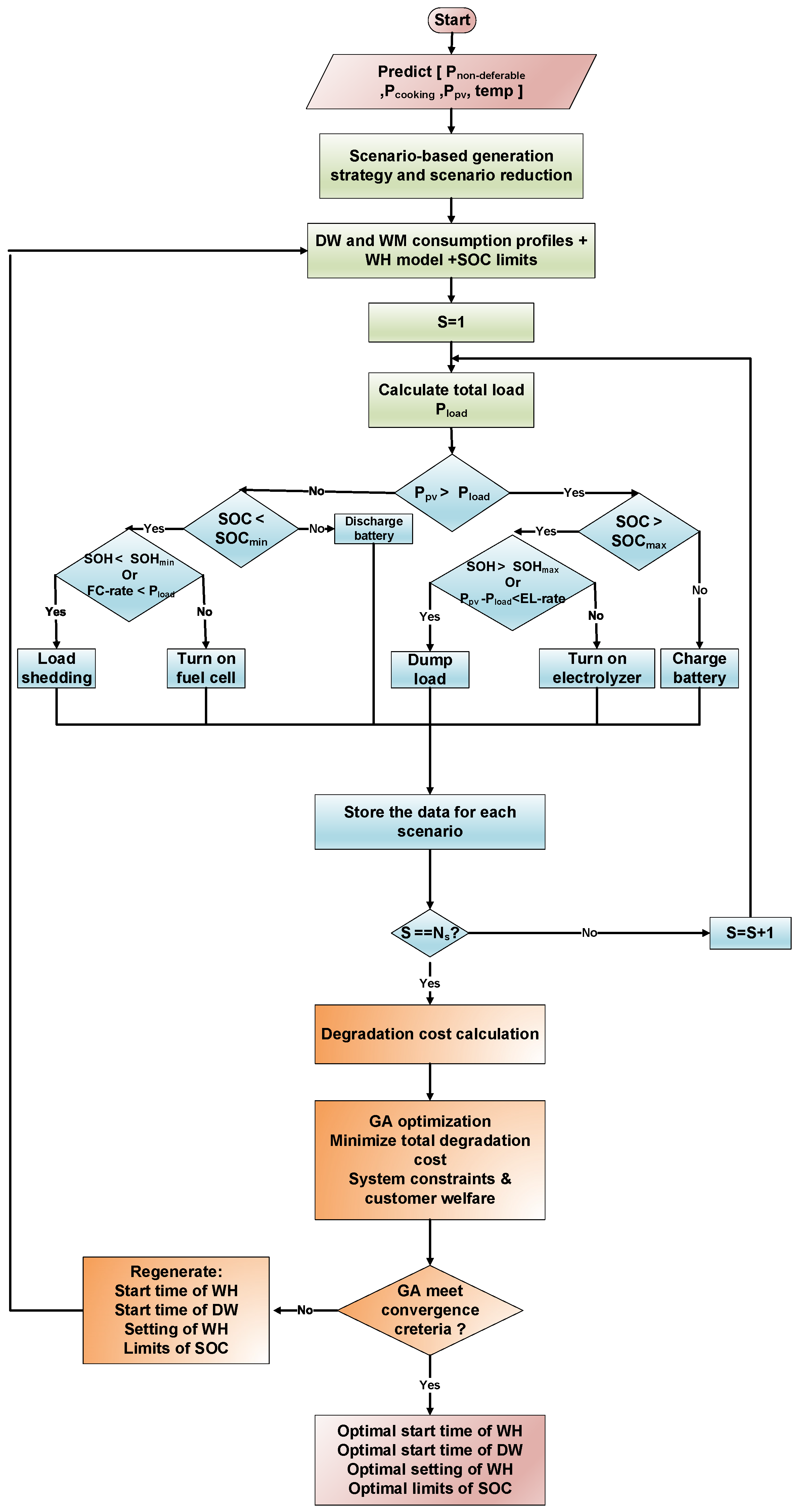
2.6. Integrated Stochastic Optimization Model and Energy Management Architecture

The main objective of the proposed SDSM technique is to minimize the operational cost associated with generating electricity and hydrogen for a self-sufficient system powered by a PV source in rural areas. Moreover, customer welfare and system constraints are incorporated into the optimization problem. Since the system operates off-grid, the operational cost is primarily determined by the degradation costs of key components such as the battery, PEM electrolyzer, and fuel cell. The proposed SDSM strategy addresses the uncertainty of load demand prediction via a scenario-based stochastic optimization framework. As explained in previous sections, load demand scenarios are generated to ensure robust performance of the proposed SDSM technique across all possibilities. The optimization problem is formulated as follows:

$$Minimize C_{total}={\displaystyle \frac{1}{N_s}}{\sum }_{s=1}^{N_s}{\pi }_s({\mathrm{C}}_{B-aging,s}+C_{deg,FC,s} +C_{deg,EL,s})$$

(29)

where $C_{total}$ (USD) is the total daily degradation cost averaged over $N_s$ scenarios to account for load profile uncertainty, ${\pi }_s$ is the probability of scenario s, and $N_s$ is the total number of scenarios. The optimization process is subject to the following constraints:

The power balance constraint ensures supply power meets demand at any time t is expressed as

$$P_{PV,t}+P_{FC,t}+P_{B-dis,t}+P_{shed,t}=P_{load,t}+P_{B-chg,t}+P_{EL,t}+P_{dump,t} , \forall t$$

(30)

Battery SOC constraints are

$$SO{C}_{min}\le SOC\le SO{C}_{max},\forall t$$

(31)

$$SO{C}_{initial}\le SO{C}_{final}$$

(32)

Moreover, the minimum and maximum limits of SOC are optimized in the proposed strategy to permit more flexibility in the operation of battery, PEM electrolyzer, and fuel cell. The constraints on the SOC limits are given below:

$$20\le SO{C}_{min}\le 40$$

(33)

$$60\le SO{C}_{max}\le 90$$

(34)

The power output constraints of the battery, PEM electrolyzer, and fuel cell are as follows:

$$\left|P_B\right|\le P_{B, max},\forall t$$

(35)

$$0\le P_{EL,t}\le P_{EL,max},\forall t$$

(36)

$$0\le P_{FC,t}\le P_{FC,max},\forall t$$

(37)

The hydrogen storage constraint that ensures hydrogen storage does not exceed tank capacity is

$$0\le SO{H}_t\le SO{H}_{max},\forall t$$

(38)

The water heater setting constraints are given below:

$$2\le \Delta T_{tolerance}\le 20$$

(39)

$$T_{set point}\le 80°$$

(40)

Dump load and load shedding constraints are

$$P_{dump,t}\le 0.04,\forall t$$

(41)

$$P_{shed,t}\le 0.04,\forall t$$

(42)

The following constraints define customer welfare in terms of allowable times to start DW and WM and the acceptable temperature for hot water demand from the WH:

$$10:00 \mathrm{AM}\le star{t}_{DW}\le 10:00 \mathrm{PM}$$

(43)

$$10:00 \mathrm{AM}\le star{t}_{WM}\le 10:00 \mathrm{PM}$$

(44)

$$Tem{p}_t\ge 37°,\forall t$$

(45)

The proposed SDSM based on GA optimization receives the daily predicted data for the power consumption of non-deferable appliances, irradiation, and temperature. Firstly, the scenario generation algorithm accounts for the uncertainty of the consumption power of non-deferable appliances and cooking profiles. The optimized parameters, which include DW and WM starting times besides the SOC limits and water heater settings (in winter session only), are initiated. Then, for each scenario, the total daily load profile is obtained with a time slot of 15 min. The predicted PV power is compared with the total load at each time slot. If there is excessive power, the battery charges until it reaches its maximum SOC limit, and then the PEM electrolyzer operates to convert the excessive electricity into hydrogen. Moreover, the excessive energy becomes a dump load if the hydrogen tank becomes full. Conversely, battery discharge is when the PV power is less than the total load power until its SOC reaches its minimum SOC limit. After that, the fuel cell operates to supply the load. If the fuel cell rate power is less than load power or the hydrogen tank becomes empty, load shedding is necessary. This energy management technique is shown in the flowchart of Figure 9. The outputs of this stage are the daily profiles of SOC of the battery, PEM electrolyzer power, fuel cell, load shedding, and dump load. These output data are entered into the cost function calculation stage to determine this scenario’s total degradation cost. The same process is repeated for all scenarios to compute the total degradation cost according to Equation (29). Finally, stochastic optimization using GA minimizes the total degradation cost over all scenarios by obtaining the optimal WM and DW operation times, optimal WH setting, and optimal SOC limits.

In this analysis, a GA is used to investigate the multi-objective optimization problem. GA is categorized as a metaheuristic optimization scheme inspired by the principles of natural selection, which results from Darwin’s theory of evolution. It also falls under a broad spectrum of algorithms known as evolutionary algorithms. The GA is based on concepts of survival of the fittest and gradually improves solutions to an optimal solution throughout the iterations. In this study, a multi-objective GA is employed for optimizing over a 24 h time horizon, creating a population of random selections of individuals. Each iteration performs a one-point crossover operator to the selected genes, which combines the genes to search and explore new landscapes for solutions. After crossover, mutation is applied to limit homogeneity of the population. A new objective function is conducted with the new individuals, where the individuals with the lowest objective value will be retained and selected for reproduction into the next generation. This process is continued iteratively for the predetermined number of generations, and the GA continues toward a near-global optimal solution [45].

2.7. Economic Indicator: Levelized Cost of Energy

The LCOE highlights the proposed approach’s benefit in reducing energy costs. LCOE is determined based on the following equation [46].

$$LCOE={\displaystyle \frac{I_{total}+NP{V}_{OM}+NP{V}_{rep}}{E_{d,total}}}$$

(46)

where $I_{total}$ (USD) is the total investment cost, $NP{V}_{rep}$ (USD) is the net present value of replacement cost, $NP{V}_{OM}$(USD) is the net present value of operational and maintenance costs, and $E_{d,total}$ (kWh) is the total energy demand during the lifetime of the system. The total investment cost is obtained by summing all component costs as follows.

$$I_{total}=C_{\mathrm{PV}} P{V}_{rated}+C_{\mathrm{EL}} P_{el,rated}+C_{\mathrm{FC}}{P}_{fc,rated}+C_{\mathrm{B}} E_{battery}+C_{\mathrm{Tank}} Tan{k}_{H2}$$

(47)

where $C_{\mathrm{PV}}$ (USD/kW) is the cost of PV panels per kW, and $C_{\mathrm{Tank}}$ (USD/kg) is the cost of 1 kg of hydrogen tank. The net present value for operational and maintenance costs is given by

$$NP{V}_{OM}=C_{\mathrm{annual}\mathrm{OM}}{\displaystyle \frac{1-{\left(1+r\right)}^{-T_{project}}}{r}}$$

(48)

where $C_{\mathrm{annual}\mathrm{OM}}$ (USD) is the annual cost of operational and maintenance that assumed 1% of investment cost, $r$ (%) is the discount rate and considered as 5% in the current study, and $T_{project}$ (years) is the total lifetime of the system (25 years). The following equation determines the replacement number of primary components, including battery, fuel cell, and PEM electrolyzer.

$$N_{rep}=\max (0, {\displaystyle \lfloor \frac{T_{project}}{T_{component}}\rfloor }-1)$$

(49)

where $T_{component}$ (years) is the component lifetime that calculated for each component as follows:

$$T_{bat}={\displaystyle \frac{1}{\Delta T^{cal}+\frac{365 {\mathrm{C}}_{B-aging}}{C_{\mathrm{B}} E_{battery}}}}$$

(50)

$$T_{FC}={\displaystyle \frac{C_{\mathrm{FC}} P_{fc,rated}}{365\times C_{deg,FC}}}$$

(51)

$$T_{EL}={\displaystyle \frac{C_{\mathrm{EL}} P_{el,rated}}{365\times C_{deg,EL}}}$$

(52)

where $\Delta T^{cal}$ is the 10% annual calendar loss of battery. Then, the net present value of replacement costs of the battery, PEM electrolyzer, and fuel cells is given by

$$NP{V}_{rep}={\sum }_{k=1}^{N_{rep,B}}{\displaystyle \frac{ C_B E_{battery}}{{\left(1+r\right)}^{k{T}_{battery}}}}+{\sum }_{k=1}^{N_{rep,FC}}{\displaystyle \frac{C_{FC} P_{fc,rated}}{{\left(1+r\right)}^{k{T}_{FC}}}}+{\sum }_{k=1}^{N_{rep,EL}}{\displaystyle \frac{C_{EL} P_{el,rated}}{{\left(1+r\right)}^{k{T}_{EL}}}}$$

(53)

Table 7 illustrates the system parameters that are used in computing the LOCE of the proposed system.

3. Results

The results presented in this section evaluate the performance of the proposed SDSM strategy for typical summer and winter days. The proposed SDSM strategy highlights the optimal operation schedules for deferable appliances, thermostatically controlled loads, and the hybrid hydrogen–battery storage system. The effectiveness of the proposed technique in minimizing degradation costs and enhancing system reliability is evaluated by systematically comparing the optimal operational results against randomly generated operational scenarios for the system components. The key performance indicators, including the total degradation cost of batteries, fuel cells, and PEM electrolyzers, as well as dump load percentage and load shedding percentage, were analyzed. Detailed consumption profile data for typical winter and summer days are illustrated in the previous sections.

Furthermore, solar irradiation and temperature data for these typical days, as shown in Figure 10, were extracted from the NASA database for the residential site near Abu Rudie’s city of Sinai Peninsula, Egypt [47]. It is important to note that this location experiences predominantly summer and winter seasons, with a very short transition period, which is not significant enough to influence the overall system performance in this study. The proposed SDSM method was implemented and validated through MATLAB simulations. The subsequent discussion provides a comprehensive analysis of the simulation results, demonstrating the effectiveness and performance of the proposed methodology.

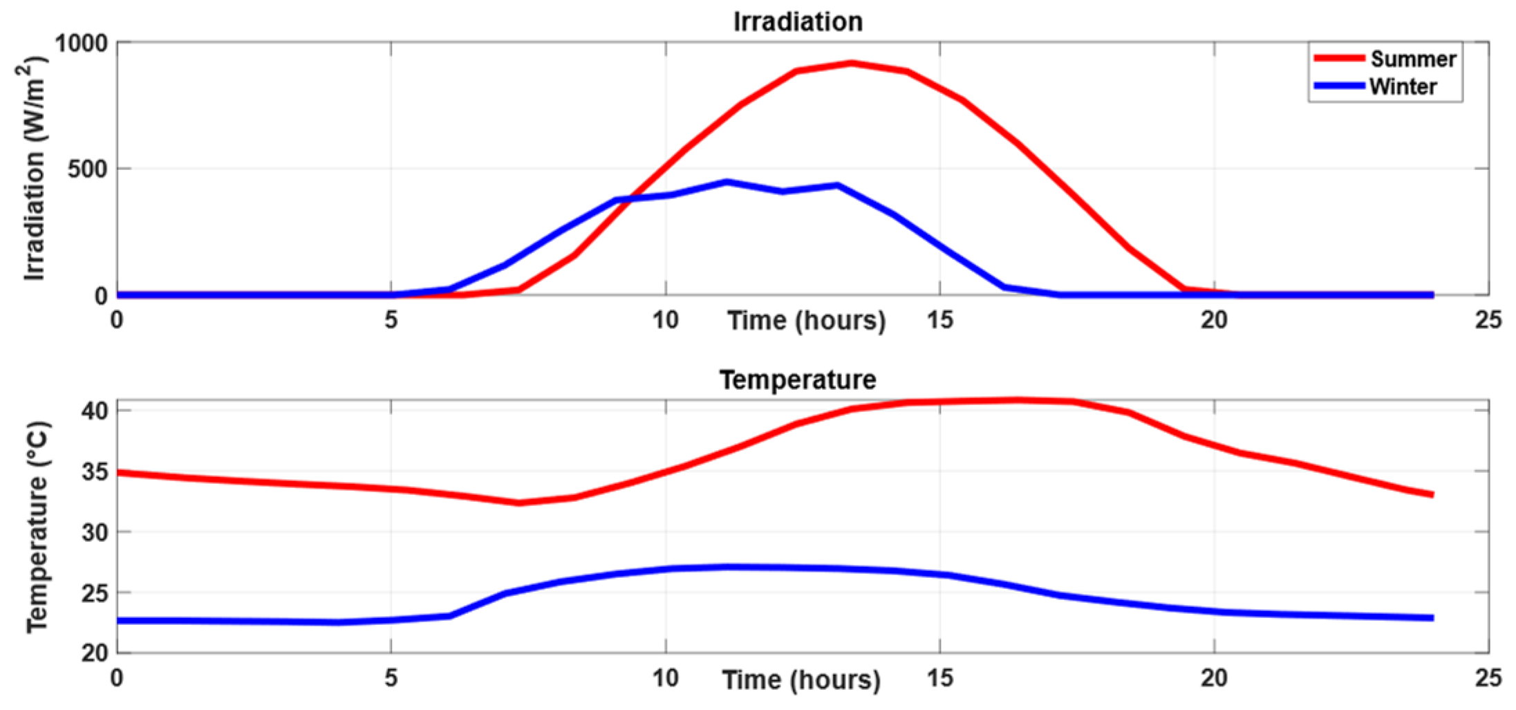
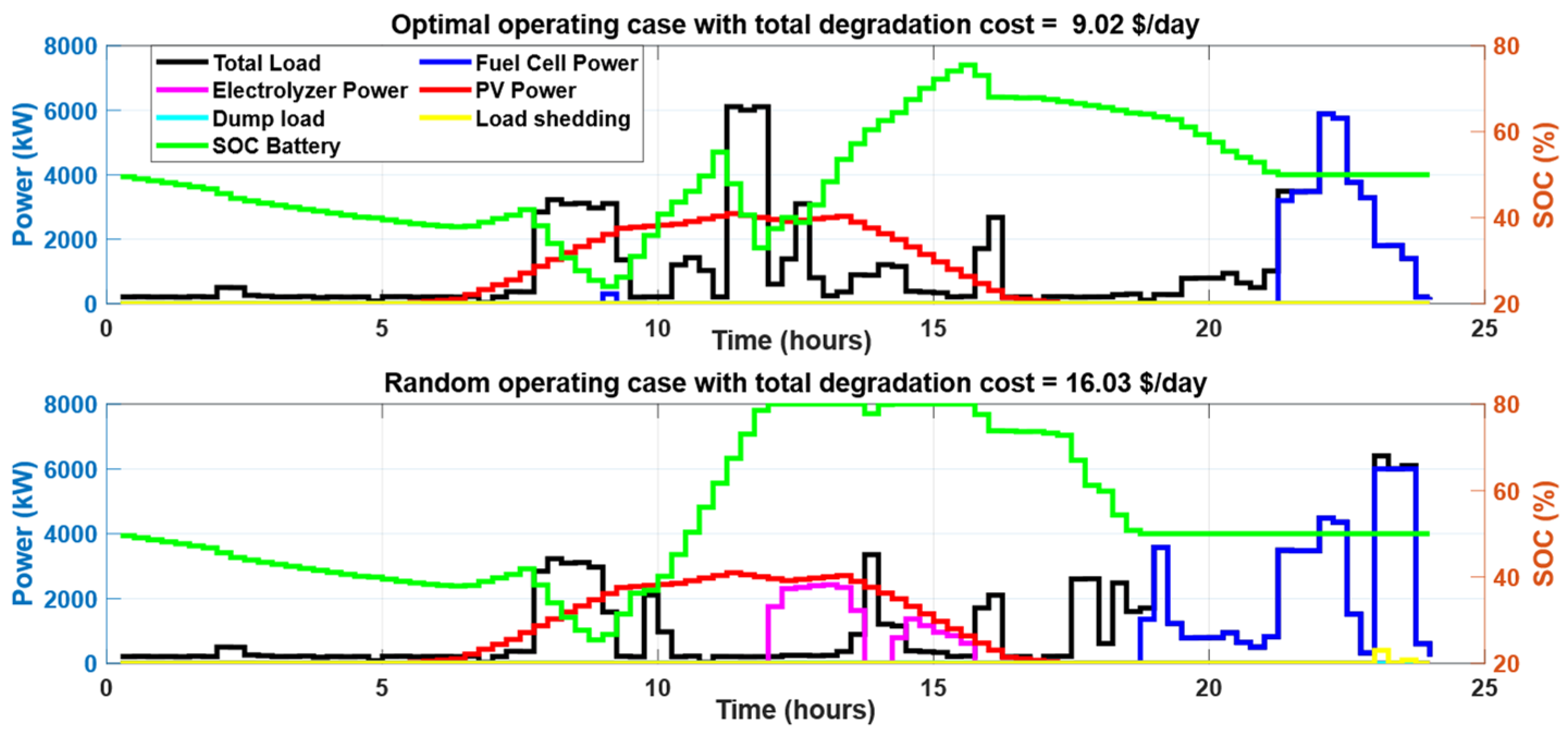
3.1. Optimal Results on Winter Day

Electric appliances that are considered in winter days include WMs, DWs, and water heaters. The proposed technique aims to determine the optimal operating times of both WMs and DWs in addition to optimal temperature set point and temperature tolerance for the water heater.

Table 8. The optimal results from the proposed SDSM technique for typical winter day.

Initial SOC of Li-Ion Battery (%)	80	70	60	50
Starting time of WM	10:15 AM	10:00 AM	10:00 AM	10:00 AM
Starting time of DW	07:45 PM	10:00 PM	10:00 PM	10:00 PM
SOC minimum (%)	22	20	24	24
SOC maximum (%)	90	90	90	90
Set point of WH	80	75	76	76
Temp. tolerance of WH	11	2	8	8
Dump load (%)	0	0	0	0
Load shedding (%)	0	0	0	0
Battery degradation cost (USD/day)	0.447	0.578	0.604	0.604
Electrolyzer degradation cost (USD/day)	1.6	0	0	0
Fuel cell degradation cost (USD/day)	8.86	8.30	6.67	8.63
Total degradation cost (USD/day)	10.91	8.81	7.28	9.23

summarizes the SDSM results for the day considered at different initial SOCs of the battery. The proposed SDSM ensures zero dumping load and zero load shedding at different initial SOCs. Figure 11 compares the power consumption profiles of different components during optimal and random operating cases at an initial SOC of 50%. The optimal operating times of shiftable loads result in lower utilization of fuel cells, no operation of the PEM electrolyzer, zero dump load, and zero load shedding. Therefore, the total degradation cost is decreased to equal 9.02 USD/day in the optimal case compared with a degradation cost of 16.03 USD/day in the considered random operation sample. The effect of initial SOC on the minimum degradation cost is illustrated in Figure 12, Figure 13 and Figure 14, where 60% initial SOC resulted in the lowest degradation cost due to the minimization of the fuel cell and PEM electrolyzer operation. To compare the optimal operation condition with random operation scenarios, the Latin hypercube sampling (LHS) method was used to generate 10,000 random scenarios by varying the start times of WMs and DWs, varying temperature tolerances and max set points, and the SOC battery limits. This method ensures an evenly distribution of generated random scenarios across the sample space [48,49,50]. Boxplots in Figure 15 summarize these results, which show a substantial impact of the proposed strategy on reducing the total degradation cost and ensuring the required constraints across different initial battery SOCs. Furthermore, the proposed SDSM results in a reduction in the total degradation cost, compared with the median of 10,000 random scenarios, equal to 30.6%, 42.8%, 53.2%, and 43.8% at initial battery SOCs equal to 80%, 70%, 60%, and 50%, respectively. By optimizing the utilization of deferrable appliances and water heaters, as well as managing the energy storage systems (Li-ion batteries and hydrogen) effectively, the presented approach achieves zero-load shedding and low-energy dumping. Load shifting and energy storage enable the system to coordinate energy supplies and demands and mitigate disruptions. In worst-case scenarios, load shedding is unavoidable, and the system must have prioritized loads in a priority list and an emergency protocol for backup to ensure end-users’ comfort. Additionally, hydrogen storage improves system reliability by providing extra backup capacity during extended periods of low renewable generation, such as during extreme weather conditions.

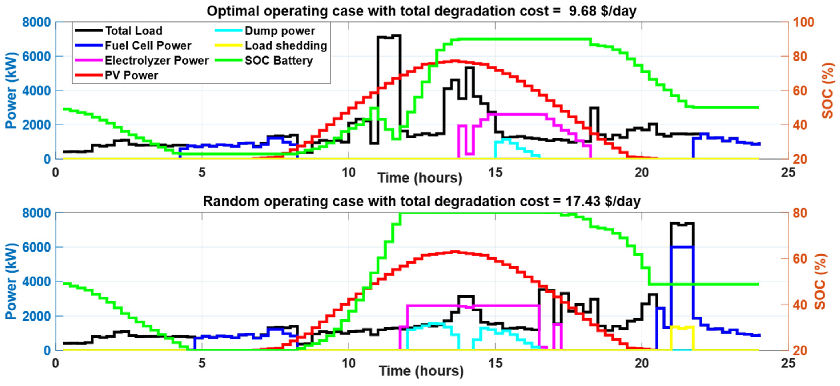
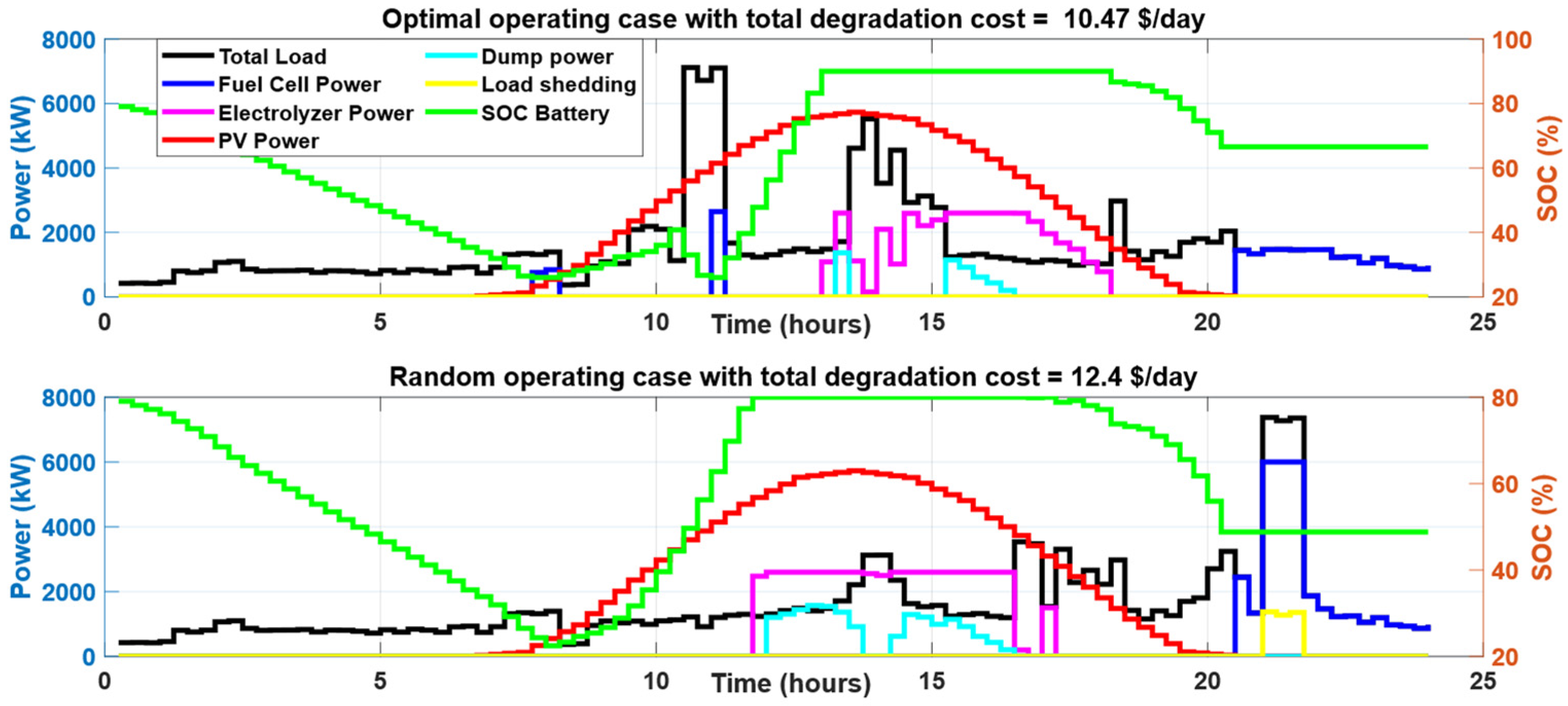
3.2. Optimal Results on a Summer Day

During summer days, the appliances that contribute to SDSM are WMs and DWs.

Table 9. The optimal results from the proposed SDSM technique for a typical summer day.

Initial SOC of Li-Ion Battery (%)	80	70	60	50
Starting time of WM	09:30 AM	09:45 AM	10:45 AM	10:00 AM
Starting time of DW	01:30 PM	01:30 PM	01:15 PM	01:15 PM
SOC minimum (%)	26	26	21	23
SOC maximum (%)	90	90	88	90
Dump load (%)	3.03	2.44	3.14	3.14
Load shedding (%)	0	0	0	0
Battery degradation cost (USD/day)	1.187	0.912	0.797	0.850
Electrolyzer degradation cost (USD/day)	2.363	2.162	1.847	1.847
Fuel cell degradation cost (USD/day)	7.222	8.537	7.751	6.943
Total degradation cost (USD/day)	10.773	11.612	10.396	9.641

summarizes the SDSM results for the day considered at different initial battery SOCs. The proposed SDSM ensures zero load shedding and limits the dumping loads to be lower than 4% at different initial SOCs. Figure 16 compares the power consumption profiles of different components during both the optimal case and random operating cases at an initial SOC of 50%. The optimal operating times of shiftable loads resulted in lower utilization of fuel cells and the PEM electrolyzer in addition to the minimization of dump load and zero load shedding. Therefore, the total degradation cost was decreased to 9.68 USD/day in the optimal case compared with a degradation cost of 17.43 USD/day in the considered random operation sample. The effect of initial SOC on the minimum degradation cost is illustrated in Figure 17, Figure 18 and Figure 19, where 50% initial SOC resulted in the lowest degradation cost due to the minimization of the fuel cell and PEM electrolyzer operation. To compare the optimal operation condition with random operation scenarios, the boxplots in Figure 20 summarize these results, which show a substantial impact of the proposed strategy on reducing the total degradation cost and ensuring the required constraints across different initial battery SOCs. Furthermore, the proposed SDSM resulted in a reduction in the total degradation cost, compared with the median of 10,000 random scenarios, equal to 12.6%, 8.66%, 19.5%, and 25.87% initial battery SOCs equal to 80%, 70%, 60%, and 50%, respectively.

3.3. Effect of the Proposed Technique on Component Lifetime and Cost of Electricity

The daily load profile for winter is assumed to be repeated over six months to represent the seasonal energy consumption during winter, while the daily load profile for summer is similarly repeated for six months to represent the summer season. The average degradation costs across four different initial SOCs were calculated to represent the daily degradation costs for each component during the winter and summer seasons. The annual degradation cost of each component is the average of winter and summer degradation, and the results are summarized in

Table 10. Comparison of the component’s lifetime for the proposed strategy and other random operations.

Operation Case	Using the Proposed SDSM	Average of 10,000 Random Operation Cases
Expected battery lifetime (years)	6.980	7.070
Expected fuel cell lifetime (years)	2.920	2.0
Expected electrolyzer lifetime (years)	7.314	4.653
LCOE (USD/kWh)	0.2694	0.3483

. The battery lifetime using the proposed technique was just 1% lower than the median of 10,000 random scenarios. However, the lifetimes of the PEM electrolyzer and fuel cell were prolonged by 57.2% and 46%, respectively, using the proposed technique, which validates its effectiveness in maximizing the component lifetime and hence reduces the cost of electricity. Moreover, the proposed technique results in zero load shedding and ensures a dumping load lower than 4%. The LCOE decreased to 0.2694 (USD/kWh) using the proposed SDSM method compared with 0.3483 (USD/kWh) representing the average LCOE for 10,000 random operation scenarios.

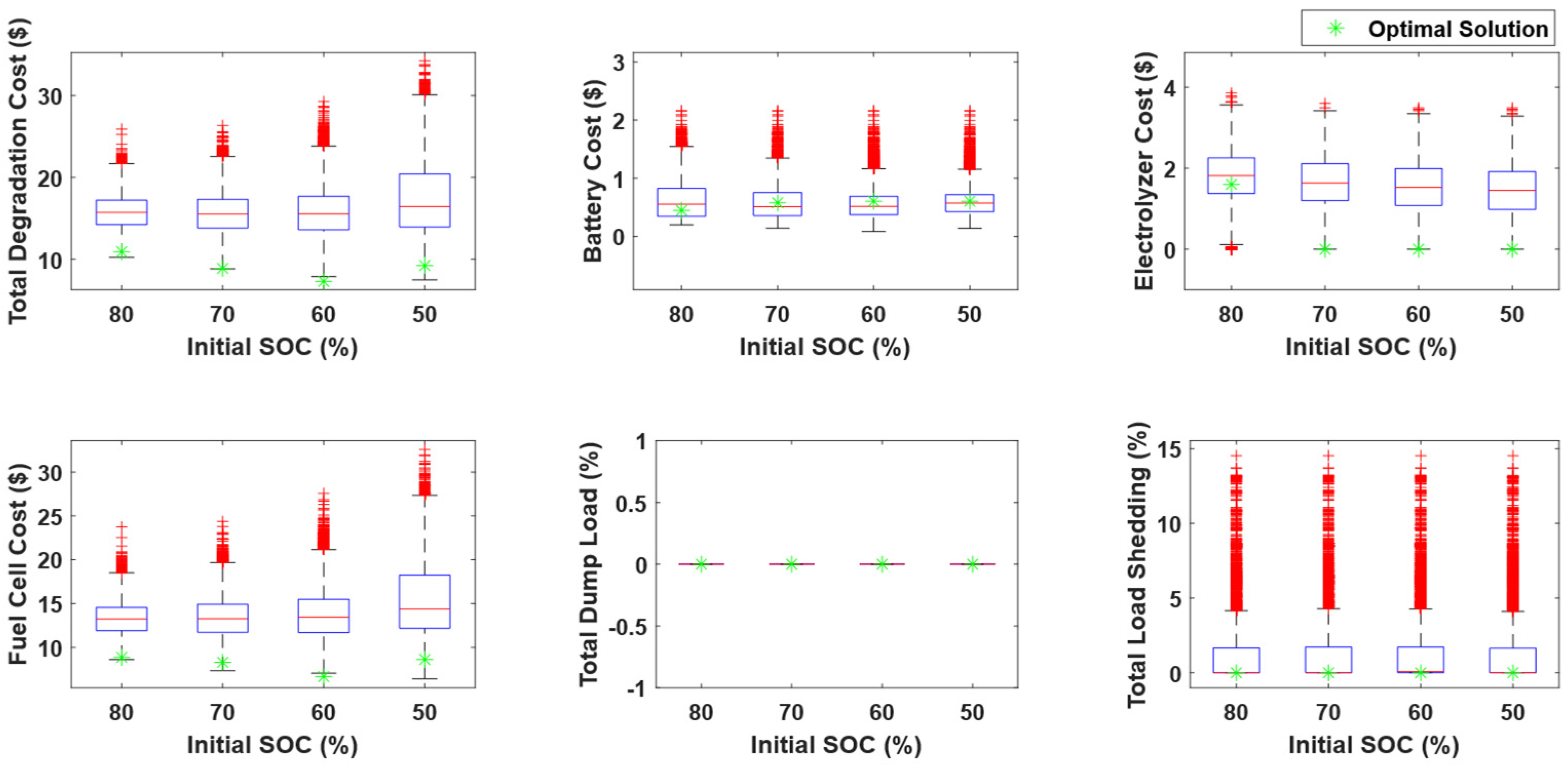
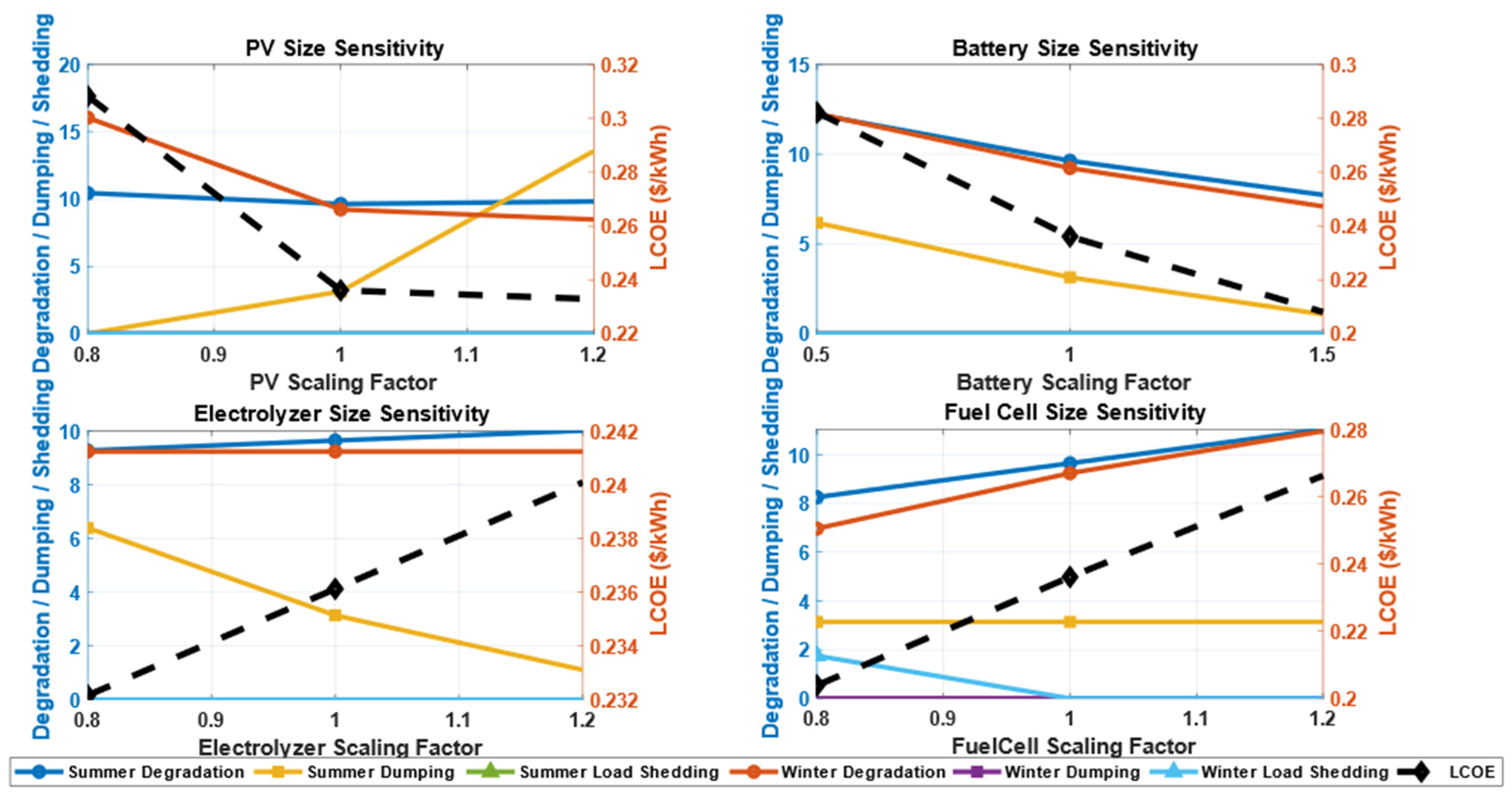
3.4. Sensitivity Analysis

The sensitivity analysis, illustrated in Figure 21, evaluated the impact of variations in key system parameters, including PV size, battery capacity, electrolyzer capacity, and fuel cell size, on critical performance metrics such as degradation costs, energy dumping, load shedding, and LCOE. This analysis will account for structural performance analysis for different sizing factors for each component, conducted in both summer and winter scenarios. For the responses from the scenarios, analyzing the size sensitivity of the PV showed that as the size increased from 0.8 to 1.2, the overall performance of the system in winter improved with less load shed and degradation. Increasing the PV size to 120% led to an energy dump, particularly in summer. The scenario of a PV size with a scaling factor of 1.2 increased the energy dumped in the summer period to 13.5%. As the PV size increased, the degradation cost decreased. This was because the increased size reduced the reliance on fuel cells in winter, causing less degradation. However, there was no effect of PV size on the degradation cost in the summer; therefore, there was no significant decrease. The LCOE reached 0.31 USD/kWh at a sizing factor of 0.8, which mostly reflected the high degradation of the fuel cells in winter when there is low PV generation and high reliance on the fuel cells. The low PV generation in winter increases the operational load on the fuel cells. It leads to high degradation costs, contributing to increases in overall LCOE at low PV capacity.

The analysis of battery size sensitivity confirmed that increasing battery size steadily reduced degradation, load shedding, and LCOE. Increasing the battery size from 50% to 150% of the optimal size reduced LCOE from 0.28 USD/kWh to 0.21 USD/kWh due to less dependence on the electrolyzer and fuel cell, which reduced their degradation. The electrolyzer size sensitivity showed little effect on degradation and dumping behaviors for increased electrolyzer size. The LCOE decreased slightly with increased electrolyzer size, decreasing from 0.238 USD/kWh at the 0.8 scaling factor to 0.233 USD/kWh at the 1.2 scaling factor. The minimal decrease in winter load shedding and energy dumping, notably in summer, did not provide sufficient economic justification for the additional cost of electrolyzers. Lastly, regarding sensitivity to fuel cell size, the load shedding was significantly decreased when considering scaling from 0.8 to 1.2, with summer shedding being reduced by as much as 2%. However, the LCOE also increased, reaching 0.26 USD/kWh when the fuel cells were scaled by a factor of 1.2. Thus, fuel cell scaling appeared beneficial in decreasing load shedding performance, while the economic costs became increasingly negative, resulting from the increase in capital and operating costs exceeding corresponding improvements.

To summarize, the analysis indicates that increasing battery capacity offers the greatest benefits from both a technical and economic standpoint due to its ability to mitigate load shedding and increase reliability; however, when increasing the size of PV or fuel cells, the potential inefficiencies of diminishing returns on energy utilization, as the components increase in size and LCOE, must be considered. The expansion of electrolyzers also shows minimal benefits compared to the costs associated with increasing size, making the electrolyzer element a relatively less favorable means of scaling. These conclusions can assist in understanding how the application system can be optimized for both performance and cost in the future.

4. Conclusions

This study proposes a novel SDSM strategy for residential off-grid PV systems integrated with hybrid Li-ion batteries and hydrogen storage. This strategy aims to minimize the total degradation costs of the battery, fuel cell, and PEM electrolyzer, while reducing energy dumping and load shedding. The proposed method optimally schedules the deferrable loads and determines the optimal setting of the water heater. The SDSM method also optimizes the battery SOC limits to enhance the flexibility of the battery, fuel cell, and PEM electrolyzer’s operation. Moreover, the uncertainty associated with load prediction is addressed through scenario-based generation to improve the accuracy and robustness of the proposed strategy. MATLAB simulations were conducted to validate the proposed approach, yielding promising results. The proposed SDSM strategy reduced the total degradation costs, compared with an average of 10,000 random operational scenarios, by 16% and 46% for typical summer and winter days, respectively. Additionally, the proposed method maintains load shedding below 4% and eliminates dumping energy. This reduction in the total degradation cost reduced the LCOE to 0.2694 (USD/kWh) compared with 0.3483 (USD/kWh) obtained from an average of 10,000 random scenarios. Sensitivity analysis indicated that increasing battery capacity provided the greatest benefits in improving system performance and reducing costs, while expanding PV, fuel cells, and electrolyzers may lead to diminishing returns and increased costs. The results highlight the practical and economic benefits of the proposed strategy, establishing it as a viable solution for enhancing the efficiency, reliability, and sustainability of off-grid PV systems integrated with hybrid Li-ion battery and hydrogen storage for powering residential loads in rural areas [51,52,53].

References

1. Choudhury, S.; Parida, A.; Pant, R.M.; Chatterjee, S. GIS augmented computational intelligence technique for rural cluster electrification through prioritized site selection of micro-hydro power generation system. Renew. Energy 2019, 142, 487–496. [Google Scholar] [CrossRef]
2. Grosspietsch, D.; Saenger, M.; Girod, B. Matching decentralized energy production and local consumption: A review of renewable energy systems with conversion and storage technologies. Wiley Interdiscip. Rev. Energy Environ. 2019, 8, e336. [Google Scholar] [CrossRef]
3. Li, N.; Lukszo, Z.; Schmitz, J. An approach for sizing a PV–battery–electrolyzer–fuel cell energy system: A case study at a field lab. Renew. Sustain. Energy Rev. 2023, 181, 113308. [Google Scholar] [CrossRef]
4. Balat, M. Potential importance of hydrogen as a future solution to environmental and transportation problems. Int. J. Hydrogen Energy 2008, 33, 4013–4029. [Google Scholar] [CrossRef]
5. Kovač, A.; Paranos, M.; Marciuš, D. Hydrogen in energy transition: A review. Int. J. Hydrogen Energy 2021, 46, 10016–10035. [Google Scholar] [CrossRef]
6. Dodds, P.E.; Staffell, I.; Hawkes, A.D.; Li, F.; Grünewald, P.; McDowall, W.; Ekins, P. Hydrogen and fuel cell technologies for heating: A review. Int. J. Hydrogen Energy 2015, 40, 2065–2083. [Google Scholar] [CrossRef]
7. Moreno-Soriano, R.; Soriano-Moranchel, F.; Flores-Herrera, L.A.; Sandoval-Pineda, J.M.; De Guadalupe González-Huerta, R. Thermal efficiency of oxyhydrogen gas burner. Energies 2020, 13, 5526. [Google Scholar] [CrossRef]
8. Bielmann, M.; Vogt, U.F.; Zimmermann, M.; Züttel, A. Seasonal energy storage system based on hydrogen for self sufficient living. J. Power Sources 2011, 196, 4054–4060. [Google Scholar] [CrossRef]
9. Fumey, B.; Stoller, S.; Fricker, R.; Weber, R.; Dorer, V.; Vogt, U.F. Development of a novel cooking stove based on catalytic hydrogen combustion. Int. J. Hydrogen Energy 2016, 41, 7494–7499. [Google Scholar] [CrossRef]
10. Topriska, E.; Kolokotroni, M.; Dehouche, Z.; Wilson, E. Solar hydrogen system for cooking applications: Experimental andnumerical study. Renew. Energy 2015, 83, 717–728. [Google Scholar] [CrossRef]
11. Scott, M.; Powells, G. Sensing hydrogen transitions in homes through social practices: Cooking, heating, and the decomposition of demand. Int. J. Hydrogen Energy 2020, 45, 3870–3882. [Google Scholar] [CrossRef]
12. Schmidt, O.; Gambhir, A.; Staffell, I.; Hawkes, A.; Nelson, J.; Few, S. Future cost and performance of water electrolysis: An expert elicitation study. Int. J. Hydrogen Energy 2017, 42, 30470–30492. [Google Scholar] [CrossRef]
13. Krishnan, S.; Koning, V.; de Groot, M.T.; de Groot, A.; Mendoza, P.G.; Junginger, M.; Kramer, G.J. Present and future cost of alkaline and PEM electrolyser stacks. Int. J. Hydrogen Energy 2023, 48, 32313–32330. [Google Scholar] [CrossRef]
14. Maharjan, S.; Zhang, Y.; Gjessing, S.; Tsang, D.H.K. User-centric demand response management in the smart grid with multiple providers. IEEE Trans. Emerg. Top. Comput. 2017, 5, 494–505. [Google Scholar] [CrossRef]
15. Al Essa, M.J.M. Home energy management of thermostatically controlled loads and photovoltaic-battery systems. Energy 2019, 176, 742–752. [Google Scholar] [CrossRef]
16. Lokeshgupta, B.; Sivasubramani, S. Multi-objective home energy management with battery energy storage systems. Sustain. Cities Soc. 2019, 47, 101458. [Google Scholar] [CrossRef]
17. Panda, S.; Mohanty, S.; Rout, P.K.; Sahu, B.K.; Bajaj, M.; Zawbaa, H.M.; Kamel, S. Residential Demand Side Management model, optimization and future perspective: A review. Energy Rep. 2022, 8, 3727–3766. [Google Scholar] [CrossRef]
18. Aljohani, T.M. Multilayer Iterative Stochastic Dynamic Programming for Optimal Energy Management of Residential Loads with Electric Vehicles. Int. J. Energy Res. 2024, 2024, 6842580. [Google Scholar] [CrossRef]
19. Sridhar, A.; Honkapuro, S.; Ruiz, F.; Mohammadi-Ivatloo, B.; Annala, S.; Wolff, A. Aggregator decision analysis in residential demand response under uncertain consumer behavior. J. Clean. Prod. 2025, 495, 144997. [Google Scholar] [CrossRef]
20. Aatabe, M.; El Abbadi, R.; Vargas, A.N.; Bouzid, A.E.M.; Bawayan, H.; Mosaad, M.I. Stochastic Energy Management Strategy for Autonomous PV-Microgrid Under Unpredictable Load Consumption. IEEE Access 2024, 12, 84401–84419. [Google Scholar] [CrossRef]
21. Yi, T.; Li, Q.; Zhu, Y.; Shan, Z.; Ye, H.; Xu, C.; Dong, H. A hierarchical co-optimal planning framework for microgrid considering hydrogen energy storage and demand-side flexibilities. J. Energy Storage 2024, 84, 110940. [Google Scholar] [CrossRef]
22. Karimi, H. A tri-objectives scheduling model for renewable-hydrogen-based microgrid system considering hydrogen storage system and demand-side management. Int. J. Hydrogen Energy 2024, 68, 1412–1422. [Google Scholar] [CrossRef]
23. Youssef, A.R.; Abdelkareem, R.; Mousa, H.H.H.; Ismeil, M.A. Economic and Technical Evaluation of Hydrogen Storage in Hybrid Renewable Systems with Demand-Side Management: Upper Egypt Case Study. IEEE Access 2024, 12, 120250–120272. [Google Scholar] [CrossRef]
24. Javid, S.S.M.; Derakhshan, G.; Hakimi, S.M. Energy scheduling in a smart energy hub system with hydrogen storage systems and electrical demand management. J. Build. Eng. 2023, 80, 108129. [Google Scholar] [CrossRef]
25. Yousri, D.; Farag, H.E.Z.; Zeineldin, H.; El-Saadany, E.F. Integrated model for optimal energy management and demand response of microgrids considering hybrid hydrogen-battery storage systems. Energy Convers. Manag. 2023, 280, 116809. [Google Scholar] [CrossRef]
26. Zakeri, B.; Syri, S. Electrical energy storage systems: A comparative life cycle cost analysis. Energy Rev. 2015, 42, 569–596. [Google Scholar] [CrossRef]
27. Mohsenian-Rad, H. Optimal bidding, scheduling, and deployment of battery systems in California day-ahead energy market. IEEE Trans. Power Syst. 2016, 31, 442–453. [Google Scholar] [CrossRef]
28. Xu, B.; Zhao, J.; Zheng, T.; Litvinov, E.; Kirschen, D.S. Factoring the Cycle Aging Cost of Batteries Participating in Electricity Markets. IEEE Trans. Power Syst. 2018, 33, 2248–2259. [Google Scholar] [CrossRef]
29. Hu, X.; Zou, C.; Tang, X.; Liu, T.; Hu, L. Cost-optimal energy management of hybrid electric vehicles using fuel cell/battery health-aware predictive control. IEEE Trans. Power Electron. 2020, 35, 382–392. [Google Scholar] [CrossRef]
30. Pu, Y.; Li, Q.; Zou, X.; Li, R.; Li, L.; Chen, W.; Liu, H. Optimal sizing for an integrated energy system considering degradation and seasonal hydrogen storage. Appl. Energy 2021, 302, 117542. [Google Scholar] [CrossRef]
31. Qayyum, F.A.; Naeem, M.; Khwaja, A.S.; Anpalagan, A.; Guan, L.; Venkatesh, B. Appliance Scheduling Optimization in Smart Home Networks. IEEE Access 2015, 3, 2176–2190. [Google Scholar] [CrossRef]
32. Nezhad, A.E.; Rahimnejad, A.; Gadsden, S.A. Home energy management system for smart buildings with inverter-based air conditioning system. Int. J. Electr. Power Energy Syst. 2021, 133, 107230. [Google Scholar] [CrossRef]
33. Shao, S.; Pipattanasomporn, M.; Rahman, S. Development of physical-based demand response-enabled residential load models. IEEE Trans. Power Syst. 2013, 28, 607–614. [Google Scholar] [CrossRef]
34. Pardiñas, Á.; Gómez, P.D.; Camarero, F.E.; Ortega, P.C. Demand–Response Control of Electric Storage Water Heaters Based on Dynamic Electricity Pricing and Comfort Optimization. Energies 2023, 16, 4104. [Google Scholar] [CrossRef]
35. Lombardi, F.S.; Riva, F.; Sacchi, M.; Colombo, E. Enabling combined access to electricity and clean cooking with PV-microgrids: New evidences from a high-resolution model of cooking loads. Energy Sustain. Dev. 2019, 49, 78–88. [Google Scholar] [CrossRef]
36. Najafi, M.H.; Jenson, D.; Lilja, D.J.; Riedel, M.D. Performing Stochastic Computation Deterministically. In IEEE Transactions on Very Large Scale Integration (VLSI) Systems; Institute of Electrical and Electronics Engineers Inc.: Piscataway, NJ, USA, 2019; pp. 2925–2938. [Google Scholar] [CrossRef]
37. Niknam, T.; Azizipanah-Abarghooee, R.; Narimani, M.R. An efficient scenario-based stochastic programming framework for multi-objective optimal micro-grid operation. Appl. Energy 2012, 99, 455–470. [Google Scholar] [CrossRef]
38. Wu, L.; Shahidehpour, M.; Li, T. Stochastic security-constrained unit commitment. IEEE Trans. Power Syst. 2007, 22, 800–811. [Google Scholar] [CrossRef]
39. Hendy, M.A.; Nayel, M.A. Sizing and Control of Isolated PV System for Self Sufficient House. In Proceedings of the IEEE Conference on Power Electronics and Renewable Energy, CPERE, Luxor, Egypt, 15–17 February 2023; Institute of Electrical and Electronics Engineers Inc.: Piscataway, NJ, USA, 2023. [Google Scholar] [CrossRef]
40. Vetter, J.; Novák, P.; Wagner, M.R.; Veit, C.; Möller, K.C.; Besenhard, J.O.; Winter, M.; Wohlfahrt-Mehrens, M.; Vogler, C.; Hammouche, A. Ageing mechanisms in lithium-ion batteries. J. Power Sources 2005, 147, 269–281. [Google Scholar] [CrossRef]
41. Kassem, M.; Bernard, J.; Revel, R.; Pélissier, S.; Duclaud, F.; Delacourt, C. Calendar aging of a graphite/LiFePO4 cell. J. Power Sources 2012, 208, 296–305. [Google Scholar] [CrossRef]
42. Purewal, J.; Wang, J.; Graetz, J.; Soukiazian, S.; Tataria, H.; Verbrugge, M.W. Degradation of lithium ion batteries employing graphite negatives and nickel-cobalt-manganese oxide + spinel manganese oxide positives: Part 2, chemical-mechanical degradation model. J. Power Sources 2014, 272, 1154–1161. [Google Scholar] [CrossRef]
43. Ecker, M.; Nieto, N.; Käbitz, S.; Schmalstieg, J.; Blanke, H.; Warnecke, A.; Sauer, D.U. Calendar and cycle life study of Li(NiMnCo)O2-based 18650 lithium-ion batteries. J. Power Sources 2014, 248, 839–851. [Google Scholar] [CrossRef]
44. Papakonstantinou, G.; Algara-Siller, G.; Teschner, D.; Vidaković-Koch, T.; Schlögl, R.; Sundmacher, K. Degradation study of a proton exchange membrane water electrolyzer under dynamic operation conditions. Appl. Energy 2020, 280, 115911. [Google Scholar] [CrossRef]
45. Torkan, R.; Ilinca, A.; Ghorbanzadeh, M. A genetic algorithm optimization approach for smart energy management of microgrid. Renew. Energy 2022, 197, 852–863. [Google Scholar] [CrossRef]
46. Bhandari, R. Standalone electricity supply system with solar hydrogen and fuel cell: Possible to get rid of storage batteries? Int. J. Hydrogen Energy 2024, 104, 599–610. [Google Scholar] [CrossRef]
47. Available online: https://power.larc.nasa.gov/data-access-viewer (accessed on 15 January 2024).
48. Sheikholeslami, R.; Razavi, S. Progressive Latin Hypercube Sampling: An efficient approach for robust sampling-based analysis of environmental models. Environ. Model. Softw. 2017, 93, 109–126. [Google Scholar] [CrossRef]
49. Yang, M.; Jiang, Y.; Zhang, W.; Li, Y.; Su, X. Short-term interval prediction strategy of photovoltaic power based on meteorological reconstruction with spatiotemporal correlation and multi-factor interval constraints. Renew. Energy 2024, 237, 121834. [Google Scholar] [CrossRef]
50. Zhang, M.; Cai, S.; Xie, Y.; Zhou, B.; Zheng, W.; Wu, Q.; Wen, J. Supply Resilience Constrained Scheduling of MEGs for Distribution System Restoration: A Stochastic Model and FW-PH Algorithm. IEEE Trans. Smart Grid 2025, 16, 194–208. [Google Scholar] [CrossRef]
51. Zhang, T.; Zhao, W.; He, Q.; Xu, J. Optimization of Microgrid Dispatching by Integrating Photovoltaic Power Generation Forecast. Sustainability 2025, 17, 648. [Google Scholar] [CrossRef]
52. Ma, K.; Yang, J.; Liu, P. Relaying-Assisted Communications for Demand Response in Smart Grid: Cost Modeling, Game Strategies, and Algorithms. IEEE J. Sel. Areas Commun. 2020, 38, 48–60. [Google Scholar] [CrossRef]
53. Zhang, H.; Yue, D.; Dou, C.; Hancke, G.P. PBI Based Multi-Objective Optimization via Deep Reinforcement Elite Learning Strategy for Micro-Grid Dispatch with Frequency Dynamics. IEEE Trans. Power Syst. 2023, 38, 488–498. [Google Scholar] [CrossRef]
Figure 1. Off-grid residential PV system with hybrid Li-ion battery–hydrogen storage.
Energies 18 03395 g001
Figure 2. Load profiles for non-deferable appliances for typical summer and winter days.
Energies 18 03395 g002
Figure 3. The consumption power profiles of a WM and DW.
Energies 18 03395 g003
Figure 4. One-minute daily hot water consumption profile for an example day at 45 °C.
Energies 18 03395 g004
Figure 5. The effect of temperature tolerance and set point temperature on power consumption profile of water heater.
Energies 18 03395 g005
Figure 6. Reduced scenarios of power consumption profiles for cooking.
Energies 18 03395 g006
Figure 7. Typical discretization of the PDF for error in load prediction.
Energies 18 03395 g007
Figure 8. The cumulative normalized probabilities.
Energies 18 03395 g008
Figure 9. Flowchart of the proposed SDSM technique.
Energies 18 03395 g009
Figure 10. Sun irradiation and temperature for typical winter and summer days.
Energies 18 03395 g010
Figure 11. The power profile of different components during optimal operation and random operation cases at initial SOC = 50% on a typical winter day.
Energies 18 03395 g011
Figure 12. The power profile of different components during optimal operation and random operation cases at initial SOC = 60% on a typical winter day.
Energies 18 03395 g012
Figure 13. The power profile of different components during optimal operation and random operation cases at initial SOC = 70% on a typical winter day.
Energies 18 03395 g013
Figure 14. The power profile of different components during optimal operation and random operation cases at initial SOC = 80% on a typical winter day.
Energies 18 03395 g014
Figure 15. The degradation cost comparison between the optimal case and 10,000 random cases generated using the LHS method for a typical winter day.
Energies 18 03395 g015
Figure 16. The power profile of different components during optimal operation and random operation cases at initial SOC = 50% on a typical summer day.
Energies 18 03395 g016
Figure 17. The power profile of different components during optimal operation and random operation cases at initial SOC = 60% on a typical summer day.
Energies 18 03395 g017
Figure 18. The power profile of different components during optimal operation and random operation cases at initial SOC = 70% on a typical summer day.
Energies 18 03395 g018
Figure 19. The power profile of different components during optimal operation and random operation cases at initial SOC = 80% on a typical summer day.
Energies 18 03395 g019
Figure 20. The degradation cost comparison between optimal cases and 10,000 random cases generated using the LHS method for a typical summer day.
Energies 18 03395 g020
Figure 21. Sensitivity analysis of key performance indicators with respect to component sizing (PV, battery, electrolyzer, and fuel cell).
Energies 18 03395 g021