A Scalable Data-Driven Surrogate Model for 3D Dynamic Wind Farm Wake Prediction Using Physics-Inspired Neural Networks and Wind Box Decomposition

Abstract

Wake effects significantly reduce efficiency and increase structural loads in wind farms. Therefore, accurate and computationally efficient models are crucial for wind farm layout optimization and operational control. High-fidelity computational fluid dynamics (CFD) simulations, while accurate, are too slow for these tasks, whereas faster analytical models often lack dynamic fidelity and 3D detail, particularly under complex conditions. Existing data-driven surrogate models based on neural networks often struggle with the high dimensionality of the flow field and scalability to large wind farms. This paper proposes a novel data-driven surrogate modeling framework to bridge this gap, leveraging Neural Networks (NNs) trained on data from the high-fidelity SOWFA (simulator for wind farm applications) tool. A physics-inspired NN architecture featuring an autoencoder for spatial feature extraction and latent space dynamics for temporal evolution is introduced, motivated by the time–space decoupling structure observed in the Navier–Stokes equations. To address scalability for large wind farms, a “wind box” decomposition strategy is employed. This involves training separate NN models on smaller, canonical domains (with and without turbines) that can be stitched together to represent larger farm layouts, significantly reducing training data requirements compared to monolithic farm simulations. The development of a batch simulation interface for SOWFA to generate the required training data efficiently is detailed. Results demonstrate that the proposed surrogate model accurately predicts the 3D dynamic wake evolution for single-turbine and multi-turbine configurations. Specifically, average velocity errors (quantified as RMSE) are typically below 0.2 m/s (relative error < 2–5%) compared to SOWFA, while achieving computational accelerations of several orders of magnitude (simulation times reduced from hours to seconds). This work presents a promising pathway towards enabling advanced, model-based optimization and control of large wind farms.

1. Introduction

1.1. Background and Motivation

Wind energy stands as a cornerstone of the global transition towards renewable energy sources, driven by environmental concerns and governmental policies aiming for carbon neutrality [1,2]. China, for instance, has witnessed exponential growth in wind power capacity, becoming the world leader in installed capacity [3,4]. However, ensuring the economic competitiveness and grid integration capabilities of wind power remains crucial, particularly as subsidies phase out [5]. Key challenges include reducing the Levelized Cost of Energy (LCoE) and enhancing the controllability of wind farms to provide grid services [6,7,8].

A significant factor impacting both the energy yield and operational costs of wind farms is the aerodynamic wake effect [9]. Upstream turbines extract kinetic energy from the wind, creating downstream regions of reduced wind speed and increased turbulence. Turbines operating within these wakes experience substantially lower power production (losses of 10–40% observed [9]) and heightened structural fatigue due to turbulence [10]. Mitigating these adverse effects through optimized farm layouts and advanced control strategies (e.g., wake steering [11,12]) is paramount for maximizing efficiency and profitability.

Effective layout design and control necessitate predictive models that can accurately capture the complex, three-dimensional (3D), and dynamic nature of wake interactions within a wind farm. Existing modeling approaches, however, present a trade-off between accuracy and computational cost. High-fidelity computational fluid dynamics (CFD) simulations based on numerically solving the Navier–Stokes equations can provide detailed 3D dynamic flow fields but are computationally prohibitive for large wind farms and real-time applications. Faster analytical models offer computational efficiency but often sacrifice accuracy and 3D dynamic fidelity, especially under complex conditions.

1.2. Literature Review and Research Gap

Wind farm wake modeling has been extensively researched, primarily falling into three categories:

1. Parameterized analytical/engineering models: These models, such as the Jensen model [13,14], Frandsen model [15], and Gaussian-based models [16] (often integrated into tools like FLORIS/FLORIDyn [17]), offer computationally inexpensive estimations of wake effects. They typically rely on simplified assumptions (e.g., self-similarity, superposition principles) and empirical parameters. While useful for preliminary design and fast calculations, their accuracy is limited, especially under complex terrain, varying atmospheric conditions, or dynamic operation [18]. They often struggle to capture the detailed 3D structure and transient behavior of wakes.

2. High-fidelity mechanistic models: Based on computational fluid dynamics (CFD), these models numerically solve the fundamental Navier–Stokes (N-S) equations governing fluid flow [19]. Techniques like large eddy simulation (LES) [20,21] or Reynolds-averaged Navier–Stokes (RANS) can provide highly accurate, time-resolved 3D predictions of the flow field, incorporating turbine forces via actuator disk or line models (ADM/ALM) [22]. SOWFA (simulator for wind farm applications) [23], based on OpenFOAM, is a prominent example widely used as a benchmark [10]. The major drawback of CFD is its immense computational expense; simulating even moderately sized wind farms for short durations can take hours or days on high-performance computing clusters [19], rendering them unsuitable for tasks requiring rapid iteration, such as real-time control or extensive layout optimization.

3. Data-driven surrogate models: Recognizing the limitations of the above, recent research has explored using machine learning, particularly deep learning, to create surrogate models (or proxy models) that emulate the accuracy of high-fidelity simulations at a fraction of the computational cost [24,25,26]. Neural networks (NNs) have shown promise in various wind energy applications, including turbine monitoring [27], site selection [28], and wake modeling [29,30]. These models learn the complex input–output relationships directly from simulation data. However, many existing NN-based wake models are limited to predicting 2D wake velocity deficits or are trained on specific, fixed farm layouts. Developing effective NN surrogates for full 3D dynamic wake prediction across arbitrary, large wind farm layouts faces significant challenges: the high dimensionality of the flow field data, the need for large training datasets from expensive CFD runs, ensuring generalization, and scaling the approach to large, diverse wind farm layouts. While some data-driven models exist, a comprehensive framework that addresses scalability for large farms and captures detailed 3D dynamic behavior using high-fidelity data remains an active research area. Direct quantitative comparisons of accuracy metrics between this work and some prior data-driven wake models are challenging due to differences in test cases, resolutions, and reported metrics, but this framework aims to advance beyond methods limited to 2D or static predictions by providing a scalable approach for full 3D dynamic fields.

To further contextualize our contribution,

Table 1. Qualitative comparison of surrogate modeling approaches for wind farm flow simulation.

Feature/Method	Analytical Models	Data-Driven
Computational cost	Very low	Low to moderate
Accuracy	Low to moderate	High
Generalizability	High	Low
Generalizability	Moderate	Moderate to high
Training requirement	Low	Very high
Scalability	Good	Poor
Interpretability	Good	Low
Handling of local features	Limited	Good

provides a qualitative comparison of the proposed wind box approach with various existing surrogate modeling methods commonly employed in wind farm flow simulation, including analytical, data-driven, and hybrid models.

Discussion: As summarized in Table 1, analytical models [24] offer remarkable computational efficiency and generalizability across various layouts due to their parameterized nature. However, their reliance on simplified physics inherently limits their accuracy, particularly in complex flow scenarios involving multiple wake interactions and turbulent mixing. Purely data-driven approaches, such as global neural networks [25,26], can achieve high accuracy by learning complex nonlinear relationships directly from data. Nevertheless, their “black-box” nature often compromises interpretability, and more critically, their generalizability to unseen wind farm layouts is typically low, as they tend to overfit to the global flow patterns of the training configurations. Scaling these global models to large wind farms also becomes challenging due to rapidly increasing model complexity and data requirements. Hybrid models [27,28] attempt to mitigate some of these limitations by integrating physical constraints or simplified models, showing improved accuracy and generalizability compared to purely data-driven methods, but often at a higher computational cost.

In contrast, our proposed wind box approach strikes a unique balance by leveraging the strengths of data-driven modeling while addressing the critical challenges of generalizability and scalability. By decomposing the complex global wind farm flow into localized “wind box” behaviors, our method can capture high-fidelity local flow features within each box, leading to high accuracy for complex flow phenomena. Critically, because each “wind box” model is trained independently on local flow conditions, the system exhibits excellent generalizability to novel wind farm layouts. A new farm can be modeled by composing pre-trained or newly trained box models, significantly reducing the need for extensive, full-field simulations for every new configuration. This modularity also ensures excellent scalability for large wind farms, as the computational cost and model complexity do not grow polynomially with the number of turbines, and the training process for individual boxes can be highly parallelized. Furthermore, while data-driven, the localized nature of the box models provides a moderate level of interpretability, allowing insights into specific wake or interaction effects within a defined region. While the initial training data requirement for each box model is high (demanding high-resolution local simulation data), this investment is amortized over many potential applications, as the library of wind box models can be reused and combined efficiently.

Predicting the full 3D dynamic wake effects in wind farms remains a significant challenge, crucial for advanced wind farm control, layout optimization, and real-time performance assessment. While high-fidelity computational fluid dynamics (CFD) models, particularly large eddy simulations (LES) (e.g., using SOWFA), offer detailed and accurate representations of turbulent wake structures and their evolution [31,32], their computational expense makes them prohibitive for applications requiring rapid, repeated simulations, such as model predictive control or extensive design space exploration. Conversely, parameterized engineering models (e.g., Jensen, Gaussian, FLORIS) are computationally efficient, but are typically 2D or quasi-3D, offering limited information on the full 3D velocity field and struggle to accurately capture complex, transient phenomena like wake meandering or intricate partial wake interactions [16]. Recent advancements in data-driven surrogate modeling, including those employing neural networks, show great promise [33]. However, many existing data-driven wake models often focus on simplified 2D wake predictions or steady-state conditions, rather than the full 3D dynamic fields, or face substantial challenges in scalability and generalization to varying wind farm layouts and large domains due to the inherent high dimensionality of the 3D spatio-temporal flow data [34,35]. The process of generating sufficiently rich and diverse high-fidelity 3D dynamic data for training these models also presents a significant bottleneck, often requiring massive computational resources [36].

1.3. Physics-Informed Neural Networks in Energy Systems

Beyond purely data-driven or solely physics-based simulations, the paradigm of Physics-Informed Neural Networks (PINNs) has emerged as a transformative approach, integrating the governing physical laws directly into neural network models. Pioneered by Raissi et al. [37], PINNs typically embed partial differential equations (PDEs) into the neural network’s loss function, allowing the model to learn solutions that simultaneously fit observed data and adhere to fundamental physical principles. This capability has led to their rapid adoption across diverse scientific and engineering disciplines. In the field of fluid dynamics, PINNs have demonstrated considerable promise. For instance, they have been successfully applied to infer complex flow fields from sparse data [33], solve notoriously challenging incompressible Navier–Stokes equations [38], and even to develop novel turbulence models, thereby offering a data-efficient pathway to understanding and predict fluid behavior. More broadly, their applicability extends to numerous other domains. In material science, PINNs are used for predicting material properties and mechanical responses under various conditions [39]. In geophysics, they aid in seismic wave propagation modeling and subsurface characterization [40]. The impact of PINNs is particularly pronounced in energy and power systems, where complex dynamics and stringent real-time requirements demand accurate yet efficient models. For power grid systems, PINNs have been instrumental in dynamic state estimation [41], real-time stability assessment and control [42], and even for accelerated transient stability analysis by learning reduced-order models that respect underlying power flow equations. They have also found applications in renewable energy forecasting, for instance, by incorporating meteorological physics into wind or solar power prediction models to enhance accuracy and robustness [43]. Furthermore, for wind farms, while the direct application of full Navier–Stokes PINNs across large 3D domains remains computationally intensive, simplified PINN formulations have been explored for specific wake phenomena, such as learning wake recovery characteristics [44] or inferring wake parameters from limited sensor data [45]. These applications highlight the value of embedding physical knowledge to improve the generalization, robustness, and interpretability of data-driven models, especially when high-fidelity data is scarce or costly to obtain. It is against this backdrop of integrating physical insights into machine learning that our study introduces a ‘Physics-Inspired Neural Network’ framework for 3D dynamic wind farm wake simulation. While our method does not strictly enforce the full Navier–Stokes PDEs in its loss function (a computational challenge for high-resolution 3D spatio-temporal wake data), it is profoundly ‘physics-inspired’ by embedding crucial physical understanding into its architectural design and by incorporating a physically motivated regularization term in its training objective. This approach allows us to leverage the strengths of data-driven learning while benefiting from the inductive biases offered by physical principles, specifically tailored to address the complexities of high-dimensional, dynamic wind turbine wakes with an emphasis on computational efficiency and scalability.

There remains a critical need for NN architectures that are both computationally efficient and structured to capture the underlying physics effectively, along with strategies to handle the scalability requirements of real-world wind farms without requiring entirely new high-fidelity simulations for every potential farm configuration.

1.4. Contributions and Paper Organization

This paper addresses the need for a fast, accurate, and scalable dynamic wake model by proposing a data-driven surrogate modeling framework based on high-fidelity SOWFA simulations. The main contributions of this work are

• Physics-inspired neural network architecture: A novel NN architecture for dynamic wake prediction is proposed that leverages an autoencoder (AE) structure. The encoder maps the high-dimensional 3D flow field to a low-dimensional latent space, where simpler dynamics are learned to predict the temporal evolution. The decoder reconstructs the full flow field from the latent state. This design is inspired by the time–space structure of the Navier–Stokes equations, where complex spatial dependencies are coupled with temporal evolution, aiming to facilitate learning and potentially improve interpretability by separating these concerns.
• Scalable wind box decomposition: To handle large wind farms without requiring monolithic simulations, a “wind box” methodology based on domain decomposition is introduced. The farm domain is decomposed into smaller, canonical subdomains (boxes) containing either a single turbine or no turbine. Separate NN surrogate models are trained for each box type using data from these smaller, standardized configurations. These models can then be stitched together, exchanging information at their boundaries, to simulate the wake propagation across arbitrary farm layouts, significantly reducing data generation requirements and enhancing model versatility compared to training on specific large layouts.
• Efficient data generation pipeline: An efficient general-purpose batch simulation tool for SOWFA, including containerized deployment (Docker 19.03.12), Python 3.9.5 APIs for parameter control and workflow management, and automated post-processing using ParaView, was developed and implemented, enabling the efficient generation of the large datasets required for NN training from multiple SOWFA runs.
• Comprehensive validation: The proposed surrogate model is validated against SOWFA simulations for both single-turbine and multi-turbine (two-turbine via three wind boxes) scenarios under varying inflow conditions and turbine yaw angles. High accuracy in predicting the 3D velocity field dynamics is demonstrated, and the significant computational acceleration achieved is quantified, illustrating its potential for real-time applications.

Building upon the existing research, this paper introduces a novel Physics-Inspired Neural Network (PINN) framework for 3D dynamic wind farm wake prediction, specifically designed to overcome the identified limitations. In conclusion, our specialization lies in (1) achieving high-fidelity 3D dynamic wake prediction, providing the detailed flow field information crucial for advanced control and analysis, which is typically only available from expensive CFD; (2) employing a physics-inspired autoencoder-latent dynamics architecture that inherently handles the high dimensionality of 3D flow data by intelligently compressing spatial features and learning temporal evolution in a low-dimensional latent space, thereby drastically improving computational efficiency over direct end-to-end models; (3) introducing a scalable wind box decomposition methodology that enables the prediction of wakes in arbitrarily large and complex wind farm layouts by combining predictions from canonical pre-trained sub-models, thus circumventing the need for extensive re-training for every new configuration and significantly reducing the data generation burden compared to monolithic models; and (4) developing an automated, efficient SOWFA batch simulation pipeline to facilitate the systematic generation of the high-quality 3D dynamic data necessary for training. This integrated approach elevates data-driven wind farm wake modeling towards practical, real-time applications by offering an unprecedented balance of accuracy, efficiency, and scalability.

The remainder of this paper is organized as follows: Section 2 details the problem formulation and the governing equations. Section 3 describes the proposed methodology, including the SOWFA batch simulation tool, the physics-inspired neural network architecture, and the wind box decomposition strategy with boundary handling. Section 4 presents the test cases, results analysis, and validation of the surrogate model’s accuracy and speed. Finally, Section 5 summarizes the key findings, discusses limitations, and suggests directions for future research.

2. Problem Formulation and Governing Equations

The objective is to predict the time-evolving 3D wind velocity field $\mathit{u}(\mathit{x},t)$ within a wind farm domain $\mathsf{\Omega }$, influenced by inflow conditions ${\mathit{v}}_{in}$, turbine operating parameters $\mathsf{\Theta }\left(t\right)$, and potentially terrain and atmospheric stability.

2.1. Governing Physics: Navier–Stokes Equations

The underlying physics of airflow in a wind farm, assuming incompressible, viscous flow, is governed by the Navier–Stokes (N-S) equations. For turbulent flow, these are typically modeled using methods like large eddy simulation (LES), which solves filtered N-S equations. The general form of the momentum equation can be written as

$$\nabla ·\mathit{u}=0$$

(1)

$$\begin{array}{cc}\hfill {\displaystyle \frac{\partial \mathit{u}}{\partial t}}+(\mathit{u}·\nabla )\mathit{u}& =-{\displaystyle \frac{1}{\rho }}\nabla p+\nabla ·(\nu \nabla \mathit{u})+{\displaystyle \frac{1}{\rho }}\mathit{f}(\mathit{x},t;\mathsf{\Theta }\left(t\right))+\nabla ·\left(\mathit{\tau }\right)\hfill \end{array}$$

(2)

Here, $\mathit{u}(\mathit{x},t)=(u_x,u_y,u_z)$ is the velocity vector at position $\mathit{x}=(x,y,z)$ and time t, $p(\mathit{x},t)$ is the pressure field, $\rho$ is the constant air density, $\nu$ is the kinematic viscosity, $\mathit{f}(\mathit{x},t;\mathsf{\Theta }(t\left)\right)$ represents the volumetric body force exerted by the wind turbines (e.g., from an actuator disk model or actuator line model), and $\mathit{\tau }$ represents the subgrid-scale stress tensor arising from turbulence modeling (e.g., in LES). Equation (2) enforces mass conservation, while Equation (2) enforces momentum conservation. The terms on the left-hand side are the temporal acceleration and momentum advection, respectively. The terms on the right-hand side represent forces due to pressure gradient, viscous diffusion, turbine interaction, and turbulent stresses. The advection term $(\mathit{u}·\nabla )\mathit{u}$ is the primary source of nonlinearity and couples spatial variations to temporal evolution.

Solving these coupled, nonlinear partial differential equations (PDEs) requires appropriate initial conditions $\mathit{u}(\mathit{x},0)$ and boundary conditions (inflow, outflow, ground, top/sides) for the domain $\mathsf{\Omega }$. High-fidelity CFD solvers like SOWFA discretize the domain and time, and numerically approximate the solution.

2.2. Challenges and Surrogate Modeling Goal

Directly solving the N–S equations via CFD is computationally prohibitive for many practical applications. The key challenges are

• Computational cost: High-resolution requirements for capturing turbulent eddies and small time steps lead to extremely long simulation times.
• Complexity: Nonlinearity, turbulence, and tight coupling between velocity and pressure make the equations difficult to solve rapidly.
• Scalability: Computational cost increases dramatically with the size of the wind farm (number of turbines and domain volume), often super-linearly.

The goal of the surrogate model is to learn a mapping ${\mathcal{M}}_{NN}$ that approximates the time evolution dictated by the N-S solver ${\mathcal{M}}_{SOWFA}$. In a discrete time setting, this means predicting the state at the next time step $t+\Delta t$ based on the current state and inputs:

$${\mathit{X}}_{t+\Delta t}\approx {\widehat{\mathit{X}}}_{t+\Delta t}={\mathcal{M}}_{NN}({\mathit{X}}_t,{\mathit{U}}_t,{\mathit{V}}_t;\mathit{W})$$

(3)

where

• ${\mathit{X}}_t$ is the discretized state vector representing the flow field (e.g., velocity components $\mathit{u}$ on a grid) within a specific wind box at time t.
• ${\mathit{U}}_t$ represents the turbine control parameters $\mathsf{\Theta }\left(t\right)$ (like yaw angle) relevant to the specific box at time t. For an empty box, this is null.
• ${\mathit{V}}_t$ represents the inflow and boundary conditions influencing the specific box at time t. In the wind box decomposition, this is primarily the flow field information from adjacent upstream boxes.
• ${\widehat{\mathit{X}}}_{t+\Delta t}$ is the surrogate model’s prediction for the state of the box at time $t+\Delta t$.
• $\mathit{W}$ represents the trainable parameters (weights and biases) of the neural network ${\mathcal{M}}_{NN}$.

The objective is to find $\mathit{W}$ such that ${\widehat{\mathit{X}}}_{t+\Delta t}$ for each box is close to the true state ${\mathit{X}}_{t+\Delta t}$ obtained from SOWFA, while ensuring that ${\mathcal{M}}_{NN}$ is computationally very fast.

3. Methodology

The methodology integrates efficient data generation using a custom SOWFA interface, a physics-inspired neural network architecture for dynamic prediction, and a scalable wind box decomposition strategy for large farm simulation.

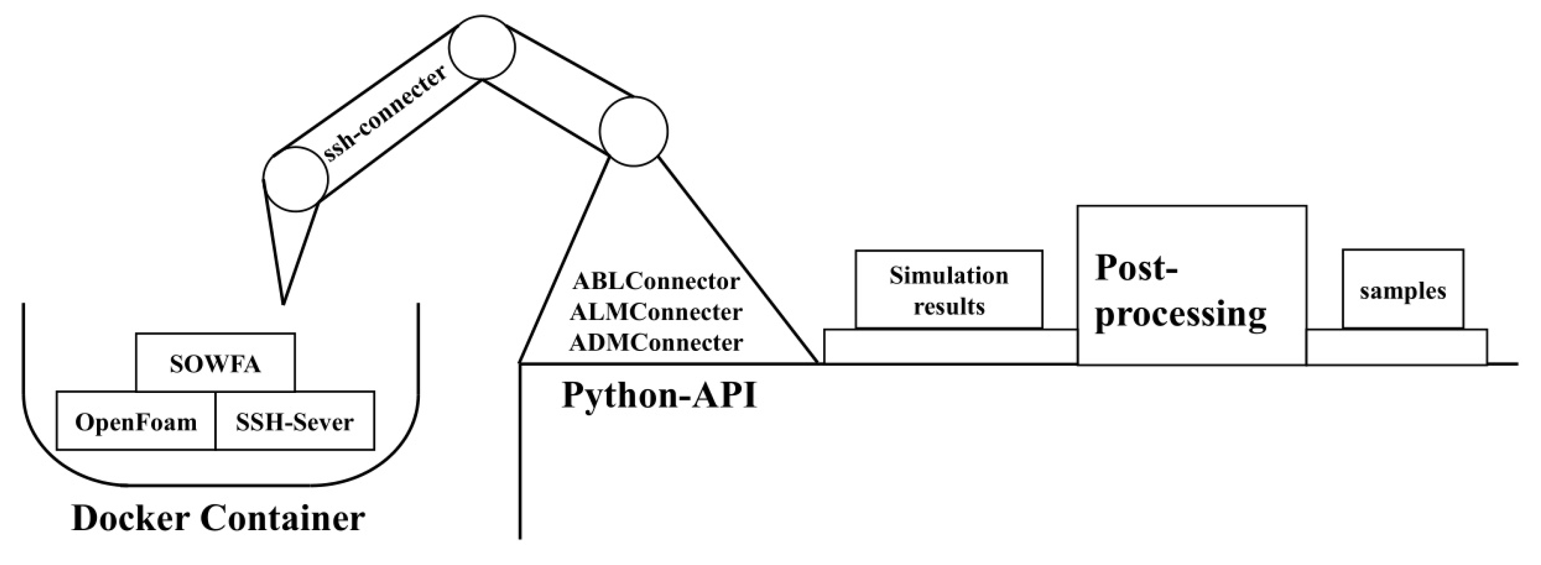
3.1. SOWFA Batch Simulation and Data Processing Tool

To generate the substantial datasets required for training the NN surrogate models, the practical challenges of using SOWFA were first addressed, namely its complex setup, cumbersome operation for multiple simulations, and lack of automated post-processing. A comprehensive batch simulation tool [46] was developed with the key following components (illustrated conceptually in Figure 1):

• Containerized SOWFA environment: Docker was utilized to create a portable SOWFA image containing all necessary dependencies (OpenFOAM, SOWFA source, compilers, etc.). This eliminates complex installations and ensures reproducibility across different computing environments. An SSH server was configured within the container for remote access and control.
• Python API for simulation management: A Python API was developed to interact with the SOWFA container via SSH. This API provides high-level functions to
  • Configure simulation parameters (e.g., wind speed, direction, turbine yaw/pitch angles, simulation time, mesh settings, and turbulence model parameters) by editing SOWFA input files based on templates. Examples of configurable parameters include mean wind speed, hub height, turbulence characteristics for ABL simulation, turbine rotor diameter, thrust and power curves, initial yaw angle, and dynamic yaw setpoints. The API includes basic validation checks for parameter ranges.
  • Manage the two-stage SOWFA simulation workflow for wind farm simulations using the actuator disk model (ADM):

    -

    ABL simulation: Simulate the atmospheric boundary layer (ABL) without turbines to generate realistic turbulent inflow conditions using LES with dynamic subgrid-scale models. The API handles setup, execution (‘ABLConnector’), and the extraction of time-varying boundary data for subsequent turbine simulations.

    -

    Turbine simulation: Introduce turbines (using ADM) into the pre-computed ABL flow and simulate the wake generation and propagation. The API (‘ADMConnector’) manages case setup based on ABL results and turbine parameters, execution, and basic checks.

  • Orchestrate batch simulations by iterating through different parameter combinations (e.g., varying mean wind speeds, yaw angles, and initial ABL states).
• Automated post-processing: The Python interface of ParaView was leveraged. Python scripts were developed to automatically:
  • Load simulation results from multiple cases.
  • Extract relevant data, such as the 3D velocity field ($\mathit{u}$) at specific time steps within defined regions (corresponding to wind boxes).
  • Sample the data onto a regular grid matching the desired NN input/output resolution.
  • Export the processed data into a format suitable for NN training (e.g., NumPy ‘.npy’ files).

This integrated toolchain significantly streamlines the process of generating large, structured datasets from SOWFA, making the data-driven approach feasible.

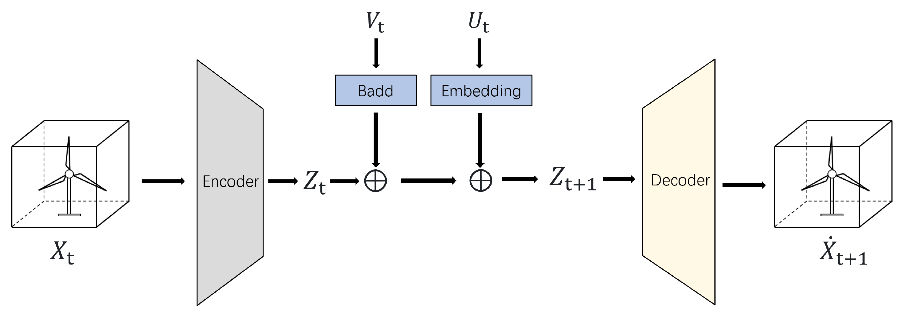
3.2. Physics-Inspired Neural Network Architecture

Directly modeling the high-dimensional spatio-temporal evolution of the wind field ${\mathit{X}}_t$ using standard recurrent NNs can be challenging due to the large state size and complex dynamics. Inspired by the structure of the N-S Equation (2), where spatial derivatives ($\nabla p$, $\nabla ·(\nu \nabla \mathit{u})$, $\nabla ·\left(\mathit{\tau }\right)$) are coupled with the temporal derivative ($\partial \mathit{u}/\partial t$) and the nonlinear advection term $(\mathit{u}·\nabla )\mathit{u}$, an NN architecture is proposed that attempts to decouple the learning of spatial features from temporal dynamics using an autoencoder (AE) framework combined with latent space evolution. This is motivated by the idea that the AE can learn a low-dimensional representation of the complex spatial patterns (like vortices and shear layers) while the latent dynamics model learns how these patterns translate and evolve over time, driven by inputs like turbine controls and boundary conditions. The architecture is shown in Figure 2.

The core components are

• Encoder (E): Maps the high-dimensional input state ${\mathit{X}}_t$ (the 3D velocity field on a grid within a wind box) to a low-dimensional latent vector ${\mathbf{Z}}_t=E({\mathit{X}}_t;{\mathit{W}}_E)$. This is implemented using 3D convolutional neural networks (CNNs) which are effective at capturing spatial hierarchies and patterns in volumetric data. The encoder compresses the essential spatial information of the flow field into ${\mathit{Z}}_t\in {\mathbb{R}}^{N_z}$, where $N_z$ is the dimension of the latent space ($N_z\ll \dim \left({\mathit{X}}_t\right)$). A typical encoder structure involves several 3D convolutional layers with an increasing number of filters and pooling operations (e.g., max pooling or strided convolutions) to reduce spatial dimensions, followed by flattening and fully connected layers to produce the latent vector.
• Latent dynamics model ($F_{latent}$): Predicts the latent state at the next time step, ${\mathit{Z}}_{t+\Delta t}=F_{latent}({\mathit{Z}}_t,{\mathit{U}}_t,{\tilde{\mathit{V}}}_t;{\mathit{W}}_F)$. This module takes the current latent state ${\mathit{Z}}_t$, the turbine controls ${\mathit{U}}_t$ (if applicable), and processed boundary/inflow information ${\tilde{\mathit{V}}}_t$ as input. It is implemented using fully connected layers (MLPs). The hypothesis is that the dynamics in the learned latent space are simpler and more predictable than in the original high-dimensional space, potentially approximating an ordinary differential equation (ODE) system $\dot{\mathit{Z}}=f(\mathit{Z},\mathit{U},\tilde{\mathit{V}})$. A specific loss term ($L_{ls}$, see Section 3.4) encourages smooth evolution in the latent space.
• Decoder (D): Reconstructs the full-dimensional state prediction ${\widehat{\mathit{X}}}_{t+1}=D({\mathit{Z}}_{t+1};{\mathit{W}}_D)$ from the predicted latent state. This is implemented using 3D Transposed Convolutional Neural Networks (TCNNs), effectively reversing the operations of the encoder to generate the 3D velocity field grid. A typical decoder structure mirrors the encoder, using transposed convolutional layers and upsampling to increase spatial dimensions, culminating in a layer that outputs the desired grid size.

Specific hyperparameters for the NN architecture used in this study are detailed in Appendix A.

The Navier–Stokes equations inherently couple complex spatial dependencies (e.g., pressure gradients, viscous diffusion, turbulent stresses, and the nonlinear advection term $(\mathit{u}·\nabla )\mathit{u}$) with temporal evolution. Our architecture, by explicitly factoring the problem into spatial feature extraction (via the autoencoder) and temporal dynamics learning (in the latent space), attempts to mimic this time–space factorization. This design acts as a powerful inductive bias, simplifying the learning task by allowing the encoder to capture complex spatial patterns and the latent dynamics model to learn how these compressed patterns translate and evolve over time, driven by external forces and boundary conditions. This factorization is expected to make the learning problem more tractable and interpretable than direct high-dimensional spatio-temporal modeling.

This architecture attempts to factorize the problem: the AE (E and D) learns a static representation of the spatial structures inherent in wake flows, while $F_{latent}$ learns the temporal evolution within this compressed representation. By compressing the state, the latent dynamics model operates on a much smaller vector, significantly reducing the number of parameters and computational cost compared to recurrent models operating directly on the full grid state, and thus improving efficiency for dynamic predictions over multiple time steps. The specific mapping relationship is shown in

Table 2. Overview of the neural network architecture components.

Component	Type	Input	Output
Encoder	3D CNNs	3D velocity grid ${\mathit{X}}_t$	Latent vector ${\mathit{Z}}_t$ (e.g., $N_z$)
Latent dynamics	MLPs	Concatenated ${\mathit{Z}}_t$, ${\mathit{U}}_t$, ${\tilde{\mathit{V}}}_t$	Predicted latent vector ${\mathit{Z}}_{t+\Delta t}$
Decoder	3D TCNNs	Predicted latent vector ${\mathit{Z}}_{t+\Delta t}$	Predicted 3D velocity grid ${\widehat{\mathit{X}}}_{t+\Delta t}$ (e.g., $31\times 31\times 16\times 3$)

.

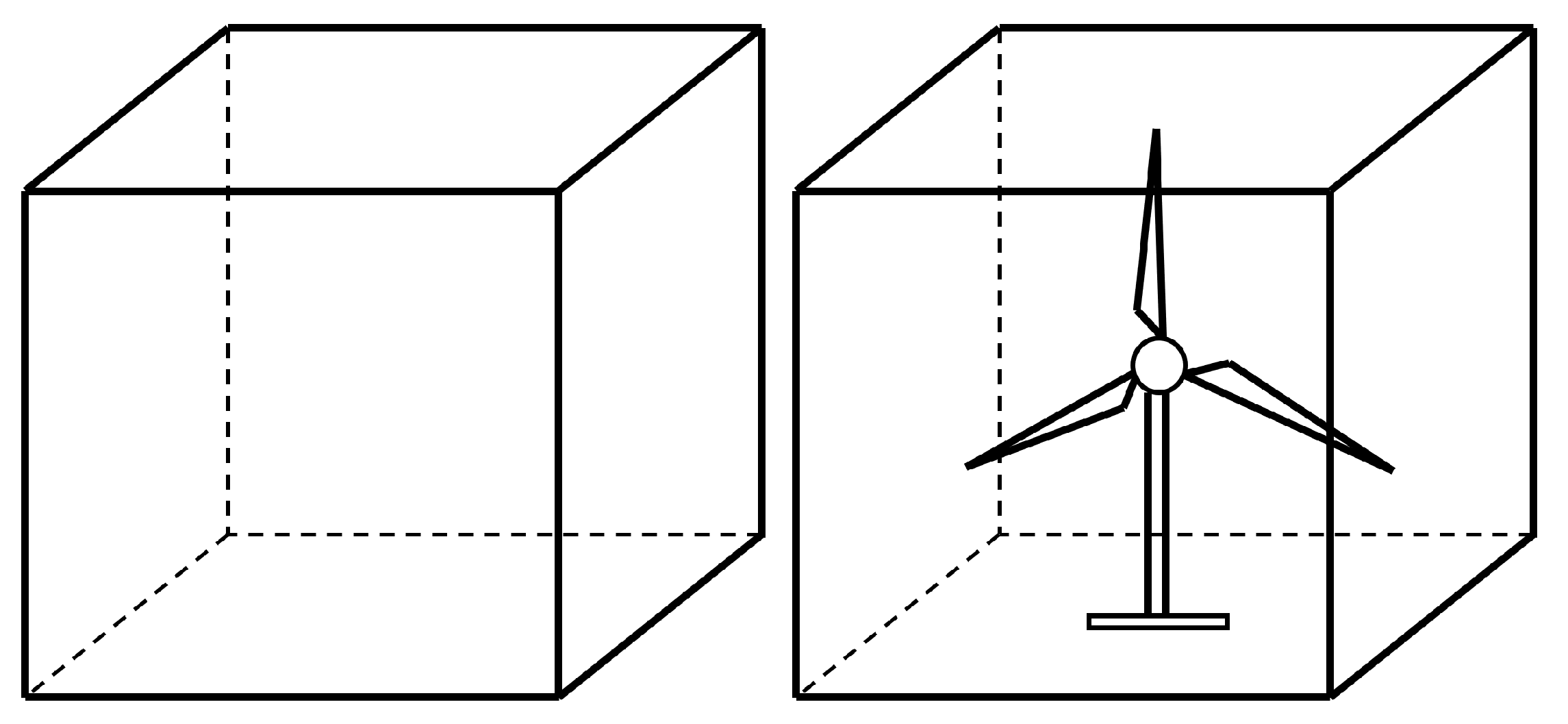
3.3. Wind Box Decomposition for Scalability

Simulating an entire large wind farm with SOWFA to generate training data for a single monolithic NN surrogate is often infeasible due to computational cost and memory limitations. Furthermore, a model trained on one specific farm layout may not generalize well to others. To address this, a “wind box” decomposition strategy based on domain decomposition principles is proposed (Figure 3).

The core idea is to divide the large wind farm domain into smaller, adjacent, or slightly overlapping, standardized cubic or cuboid regions called “wind boxes”. Two primary types of wind boxes are defined for training data generation:

• Turbine wind box (${\mathsf{\Omega }}^{WT}$): A box containing a single wind turbine centered within it. The NN model for this box (${\mathcal{M}}_{NN}^{WT}$) is trained to predict the flow evolution considering the turbine’s presence and its operating parameters (${\mathit{U}}_t$), based on uniform or pre-calculated non-uniform inflow (${\mathit{V}}_t$).
• Empty wind box (${\mathsf{\Omega }}^{NoWT}$): A box located in a region without a turbine, primarily responsible for modeling wake propagation and recovery. Its NN model (${\mathcal{M}}_{NN}^{NoWT}$) is trained to predict the flow evolution based on its upstream inflow conditions (${\mathit{V}}_t$). The governing N-S equations simplify as the turbine force term $\mathit{f}$ is zero in this region, although turbulent stresses remain.

Separate NN surrogate models (using the architecture from Section 3.2) are trained for each type of wind box using SOWFA data specifically generated for these canonical configurations under various inflow conditions (representing different ambient flows or upstream wake states) and turbine parameters (for ${\mathsf{\Omega }}^{WT}$). For ${\mathsf{\Omega }}^{NoWT}$, the training data include cases with various inflow profiles corresponding to wakes from an upstream turbine operating under different conditions.

During inference for a specific large wind farm layout, the farm domain is tiled with appropriate instances of these pre-trained wind box models. The simulation proceeds time step by time step, with each box model predicting its state based on its current state, turbine parameters (if any), and inflow conditions derived from neighboring boxes at the previous time step. The careful handling of the interface conditions (${\mathcal{B}}_{k,j}$ between box k and j) is crucial for accurate wake propagation. In the implementation for adjacent boxes aligned with the primary flow direction, the inflow condition ${\mathit{V}}_t$ for a downstream box is derived from the predicted state ${\widehat{\mathit{X}}}_{k,t}$ in the outflow region of the upstream box k at time t. Specifically, the velocity field data on multiple vertical planes at the downstream boundary region of the upstream box(es) is extracted and used as input ${\tilde{\mathit{V}}}_t$ to the latent dynamics model $F_{latent}$ of the downstream box. This captures the necessary spatial information for accurate advection across the interface, motivated by the spatial stencil dependencies of the discretized N–S schemes. For the multi-turbine case in this paper (Case 2), the interface inflow ${\tilde{\mathit{V}}}_t$ for a downstream box is constructed by concatenating sampled velocity data from 3 vertical planes located at the downstream boundary of the upstream box(es). These planes cover the full height and width of the box interface and are sampled at the same resolution as the grid within the box ($31\times 16$ points per plane). The resulting vector of velocity components from these planes becomes part of the input to the latent dynamics model. The size of the wind boxes was chosen based on the typical wake length and recovery distance, ensuring sufficient domain to capture the primary wake features while remaining computationally tractable for SOWFA training runs.

This approach offers significant advantages:

• Reduced data generation cost: SOWFA simulations are only needed for the smaller, canonical wind box configurations, rather than for every potential large farm layout. This drastically reduces the computational resources and time required for data generation.
• Scalability: Simulating large farms involves stitching together predictions from multiple smaller, fast NN models running in parallel or sequence, which is computationally much cheaper than a monolithic large-scale CFD or NN model. The total computational cost scales roughly linearly with the number of boxes.
• Versatility/generalization: Arbitrary farm layouts and potentially different turbine types (by training specific ${\mathsf{\Omega }}^{WT}$ models) can potentially be assembled using the pre-trained canonical box models, enhancing the model’s applicability to diverse farm designs, provided that the canonical training data cover the relevant inflow conditions and turbine states.

3.4. Training Procedure

Training the NN models involves finding the optimal parameters ${\mathit{W}}^{*}$ that minimize a carefully designed loss function based on the SOWFA-generated data $\mathcal{D}={\left\{({\mathit{X}}_t^{\left(i\right)},{\mathit{U}}_t^{\left(i\right)},{\mathit{V}}_t^{\left(i\right)},{\mathit{X}}_{t+\Delta t}^{\left(i\right)})\right\}}_{i=1}^{N_{samples}}$ for each box type (${\mathsf{\Omega }}^{WT}$ and ${\mathsf{\Omega }}^{NoWT}$). A two-stage training process is employed:

1. Pre-training: The autoencoder component (E and D) is pre-trained independently on all available flow field snapshots $\left\{{\mathit{X}}_t^{\left(i\right)}\right\}$ from the relevant box dataset. The goal is to learn an effective spatial compression to the latent space $\mathit{Z}$ and reconstruction back to the full grid $\mathit{X}$. The loss function is typically the mean squared error (MSE) of reconstruction:

$$L_{rec}={\displaystyle \frac{1}{N_{samples}}}\sum _{i=1}^{N_{samples}}\left|\right|{\mathit{X}}_t^{\left(i\right)}-D(E({\mathit{X}}_t^{\left(i\right)};{\mathit{W}}_E);{\mathit{W}}_D){\left|\right|}_2^2$$

(4)

This step helps initialize the AE weights to effectively capture the variance in the spatial data.

2. Formal training: The complete network (encoder, latent dynamics, decoder) is trained end-to-end to predict the state at the next time step. The loss function combines several terms to guide the learning process:

$$L_{total}={\lambda }_{pred}{L}_{pred}+{\lambda }_{rec}{L}_{rec}+{\lambda }_{ls}{L}_{ls}+R\left(\mathit{W}\right)$$

(5)

where

• $L_{pred}$: The primary prediction loss, measuring the difference between the predicted state ${\widehat{\mathit{X}}}_{t+\Delta t}$, and the true SOWFA state ${\mathit{X}}_{t+\Delta t}$. The mean squared error (MSE) of the velocity components is used:

  $$L_{pred}={\mathbb{E}}_{\mathcal{D}}\left[\right||{\mathit{X}}_{t+\Delta t}-{\widehat{\mathit{X}}}_{t+\Delta t}{\left|\right|}_2^2]$$

  (6)

  where ${\widehat{\mathit{X}}}_{t+\Delta t}=D\left(F_{latent}(E\left({\mathit{X}}_t\right),{\mathit{U}}_t,{\tilde{\mathit{V}}}_t)\right)$ and $\left|\right|·{\left|\right|}_2^2$ denotes the squared L2 norm (sum of squared differences) over all grid points and velocity components within the box.
• $L_{rec}$: The reconstruction loss (as in Equation (4)) is retained with a small weight (${\lambda }_{rec}$) to ensure that the AE component remains effective in finding meaningful latent representations during end-to-end training.
• $L_{ls}$: A latent space regularization term encouraging smooth evolution in the learned dynamics. As used in this work, this penalizes large second-order differences in the latent space, encouraging a behavior similar to a simple discrete time integration step:

  $$L_{ls}={\mathbb{E}}_{\mathcal{D}}\left[\right||E\left({\mathit{X}}_{t+\Delta t}\right)+E\left({\mathit{X}}_{t-\Delta t}\right)-2E\left({\mathit{X}}_t\right){\left|\right|}_2^2]$$

  (7)
  This term aims to make the learned latent dynamics $F_{latent}$ locally approximate linear dynamics, making the latent space trajectories smoother and potentially more predictable. This is conceptually related to ensuring that velocity in the latent space ($E\left({\mathit{X}}_{t+\Delta t}\right)-E\left({\mathit{X}}_t\right)$) changes smoothly over time, rather than exhibiting sudden jumps or chaotic behavior, which can improve the stability of multi-step rollouts.
• $R\left(\mathit{W}\right)$: An optional weight regularization term (e.g., L2) to prevent overfitting, ${\lambda }_{L2}{\left|\right|\mathit{W}\left|\right|}_2^2$.

A latent space regularization term encouraging smooth evolution in the learned dynamics. As used in this work, this penalizes large second-order differences in the latent space, calculated as shown. This term aims to regularize the latent space evolution, encouraging a behavior analogous to smooth temporal integration or a stable physical system. Specifically, it promotes that the ‘velocity’ of the latent state changes smoothly over time, rather than exhibiting sudden jumps or chaotic behavior. This implicitly guides the latent dynamics model $F_{latent}$ towards learning trajectories that are more physically plausible and significantly improves the stability and accuracy of multi-step rollouts.

The expectation ${\mathbb{E}}_{\mathcal{D}}[·]$ is approximated by averaging over mini-batches from the training dataset. The hyperparameters ${\lambda }_{pred},{\lambda }_{rec},{\lambda }_{ls}$ control the relative importance of these objectives and were tuned based on validation set performance (e.g., using grid search). Optimization was performed using the Adam optimizer. The learning rate was decayed over training epochs. Specific training hyperparameters are provided in Appendix A.

This structured training approach, combining pre-training with a multi-objective loss function, aims to produce a surrogate model that is not only accurate in prediction but also possesses a meaningful and stable latent representation reflecting the underlying physical dynamics.

The training of each individual “wind box” model was performed on a high-performance server equipped with 2 Intel Xeon Gold 5118 processors (totaling 24 CPU cores with 48 threads) and 250 GB RAM. For a typical box type, the training process, involving approximately 50–100 epochs, converged within approximately 1 h. It is noteworthy that the training of different box types can be conducted independently and in parallel, which significantly reduces the total wall-clock time required to establish a comprehensive library of models for a given wind farm layout.

4. Test Cases and Results Analysis

The proposed methodology was evaluated through a series of test cases, progressively increasing complexity from validating the SOWFA interface to simulating dynamic wakes in single-turbine and multi-turbine (via wind box stitching) scenarios. All NN training and inference were performed on a server equipped with NVIDIA V100 GPUs. SOWFA simulations were run on a CPU cluster (Intel Xeon E5-2680 v4, 2.4 GHz).

4.1. Test Case Setup and Data Generation

Using the SOWFA batch simulation tool described in Section 3.1, datasets were generated for training and testing the NN surrogate models.

SOWFA simulation parameters:

• Turbine model: NREL 5MW reference turbine, modeled using ADM with standard parameters.
• Domain size: Varied by case. For single-box studies, canonical box dimensions were $(600\mathrm{m},600\mathrm{m},300\mathrm{m})$. For the two-turbine/three-box case, the total SOWFA simulation domain was $(1800\mathrm{m},600\mathrm{m},300\mathrm{m})$.
• Grid resolution: The SOWFA mesh used approximately $5\mathrm{m}$ resolution in the turbine and wake regions. The NN input/output grid resolution within each wind box was fixed at $31\times 31\times 16$ points (approx. $20\mathrm{m}$ spacing), sampled from the high-resolution SOWFA output using ParaView scripts.
• Atmospheric conditions: Standard neutral atmospheric boundary layer (ABL) conditions were simulated first using LES with a dynamic Smagorinsky subgrid-scale model. Turbulent inflow conditions for turbine simulations were generated using the ‘ABLConnector’ tool. Inflow mean wind speeds ranged from $7\mathrm{m}/\mathrm{s}$ to $16\mathrm{m}/\mathrm{s}$ at hub height. Turbulence intensity was approximately 8%.
• Turbine operation: Yaw angles were varied. Static cases used yaw angles like $0^{\circ },\pm {15}^{\circ },\pm {30}^{\circ }$. Dynamic cases involved step changes or continuous variations in yaw angle (e.g., changing from ${270}^{\circ }$ to ${290}^{\circ }$ or ${250}^{\circ }$ over time, assuming mean wind from ${270}^{\circ }$).
• Simulation time: Dynamic simulations typically ran for $200\mathrm{s}$ of physical time after an initial $100\mathrm{s}$ spin-up period to establish quasi-steady flow. Data snapshots of the 3D velocity field were saved every $\Delta t=2\mathrm{s}$.

Dataset preparation:

• SOWFA output (velocity fields $\mathit{u}$) was processed using the ParaView scripts, extracting the velocity components $(u_x,u_y,u_z)$ on the $31\times 31\times 16$ grid within each defined wind box volume.
• For dynamic models, each SOWFA simulation run (e.g., 100 time steps over 200 s) constituted a sequence sample. Training data consisted of pairs $({\mathit{X}}_t,{\mathit{X}}_{t+\Delta t})$ along with corresponding inputs $({\mathit{U}}_t,{\mathit{V}}_t)$ for each time step t.
• The datasets were split into training ($80\%$) and testing ($20\%$) sets at the simulation run level. For the multi-turbine case, the dataset was generated from 369 dual-turbine SOWFA runs with varying wind speeds and yaw maneuvers, yielding corresponding sequence samples for each of the three boxes.
• The dataset size of 369 runs for the two-turbine case was chosen to capture variability across different inflow speeds and yaw maneuvers for the specific box configurations used in this study under neutral ABL. Generalizing to significantly different conditions, turbine types, or more complex layouts may require expanding the training dataset to cover the necessary parameter space.

4.2. Case 1: Single Wind Turbine Dynamic Wake Prediction

Purpose: To validate the core physics-inspired NN architecture (AE + latent dynamics) for predicting the dynamic evolution of the wake behind a single turbine. Setup: A single $(600\mathrm{m},600\mathrm{m},300\mathrm{m})$ wind box containing one turbine was simulated using SOWFA under varying inflow speeds (8–16 $\mathrm{m}/\mathrm{s}$) and dynamic yaw angle changes (250°–290°). The NN model (${\mathcal{M}}_{NN}^{WT}$) was trained using the procedure in Section 3.4 to predict the velocity field ${\mathit{X}}_{t+\Delta t}$ given ${\mathit{X}}_t$, yaw angle ${\mathit{U}}_t$, and uniform turbulent inflow ${\mathit{V}}_t$. Results:

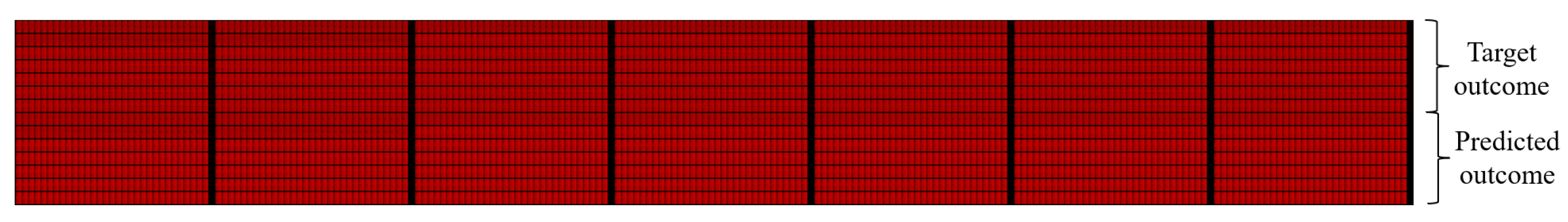
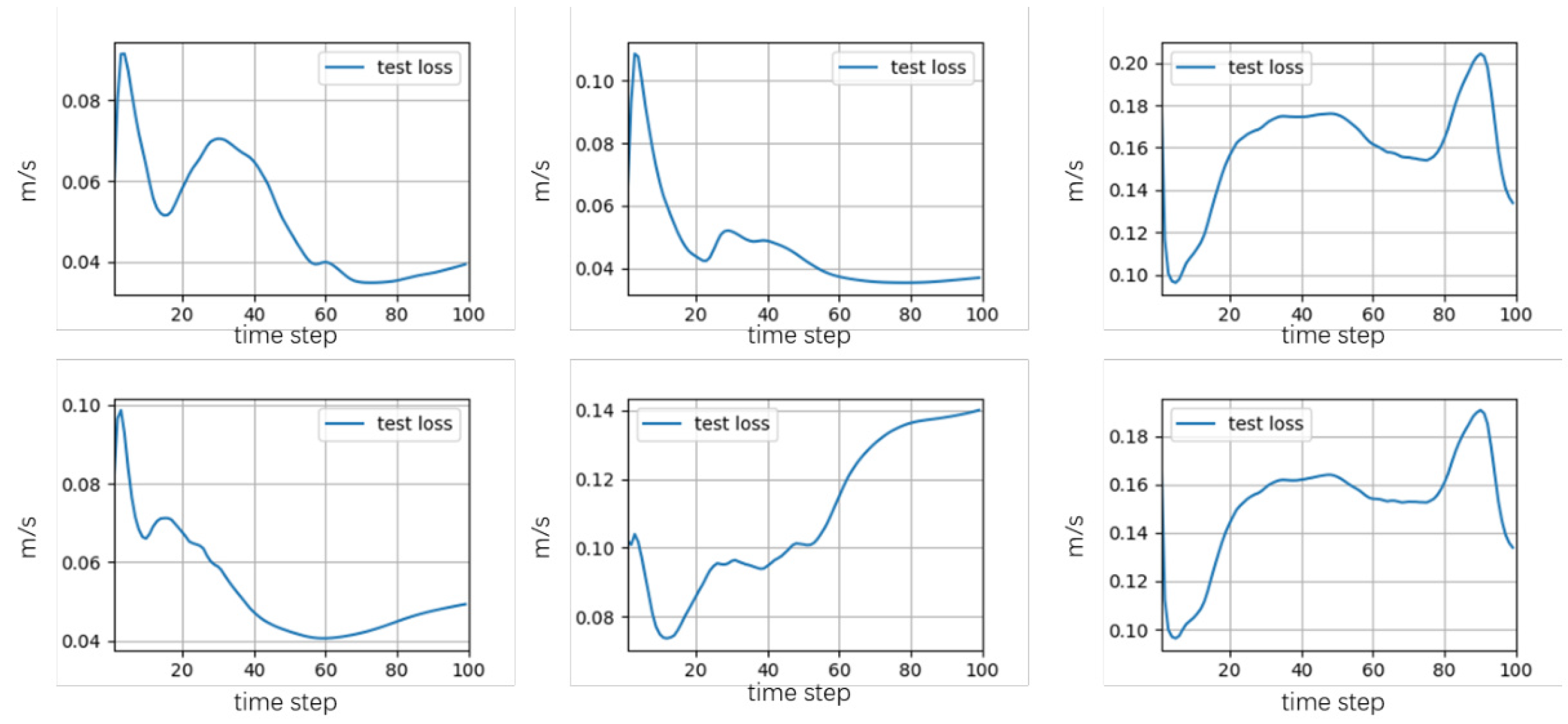
• Accuracy: The NN surrogate model demonstrated good agreement with the SOWFA results. Figure 4 shows a qualitative comparison of the velocity field on a horizontal slice at hub height for a dynamic yaw maneuver, indicating that the NN captures the main wake features like the velocity deficit shape and trajectory accurately. Figure 5 plots the average velocity error (AVE) on the test set. AVE is defined as the root mean square error (RMSE) of the three velocity components ($\sqrt{{\displaystyle \frac{1}{N_{grid}}}{\sum }_{i=1}^{N_{grid}}\left|\right|{\widehat{\mathit{u}}}_i-{\mathit{u}}_i{\left|\right|}_2^2}$) averaged over all grid points within the box, for a prediction rollout over 100 time steps (200 s physical time). The AVE remained consistently low, typically below $0.2\mathrm{m}/\mathrm{s}$ across different inflow wind speeds on the test set. The average relative error (AVE divided by the mean inflow speed) was generally below $2\%$.
• Speed: The NN model achieved significant acceleration. Simulating 200 s of physical time using a trained NN model took approximately 0.4–0.5 $\mathrm{s}$ on a V100 GPU, compared to approximately $1\mathrm{h}46\min$ for the corresponding SOWFA simulation on a multi-core CPU (Intel Xeon E5-2680 v4, 2.4 GHz, utilizing multiple cores). This represents an acceleration factor of over 10,000×.

These results validate the ability of the proposed AE + Latent Dynamics architecture to learn and rapidly predict single-turbine wake dynamics with reasonable accuracy for short-to-medium term rollouts.

4.3. Case 2: Multi-Turbine Dynamic Wake Prediction Using Wind Box Stitching

Purpose: To evaluate the scalability and accuracy of the wind box decomposition approach for modeling wake interactions in a multi-turbine setting. Setup: A two-turbine scenario was simulated using SOWFA in a larger $(1800\mathrm{m},600\mathrm{m},300\mathrm{m})$ domain, with turbines spaced $1200\mathrm{m}$ apart (approx. 10 rotor diameters) primarily aligned with the main wind direction. This domain was decomposed into three adjacent $(600\mathrm{m},600\mathrm{m},300\mathrm{m})$ wind boxes along the wind direction: Box 1 (containing Turbine 1), Box 2 (empty, modeling wake propagation), and Box 3 (containing Turbine 2, experiencing wake from Turbine 1). Separate pre-trained NN models (${\mathcal{M}}_{NN}^{WT}$ for Box 1 and 3, ${\mathcal{M}}_{NN}^{NoWT}$ for Box 2) were used. During testing, the three pre-trained models were run concurrently, exchanging boundary information at each time step. Box 1 received uniform turbulent inflow ${\mathit{V}}_t$. Box 2 received inflow ${\mathit{V}}_{2,t}$ derived from the outflow region of Box 1’s NN prediction (${\widehat{\mathit{X}}}_{1,t}$) at time t. Box 3 received inflow ${\mathit{V}}_{3,t}$ derived from the outflow region of Box 2’s NN prediction (${\widehat{\mathit{X}}}_{2,t}$) at time t. The inflow ${\tilde{\mathit{V}}}_t$ for $F_{latent}$ in Boxes 2 and 3 was constructed by sampling the predicted velocity field on three vertical planes at the upstream boundary of the respective box, as described in Section 3.3 and Appendix A.1. Results:

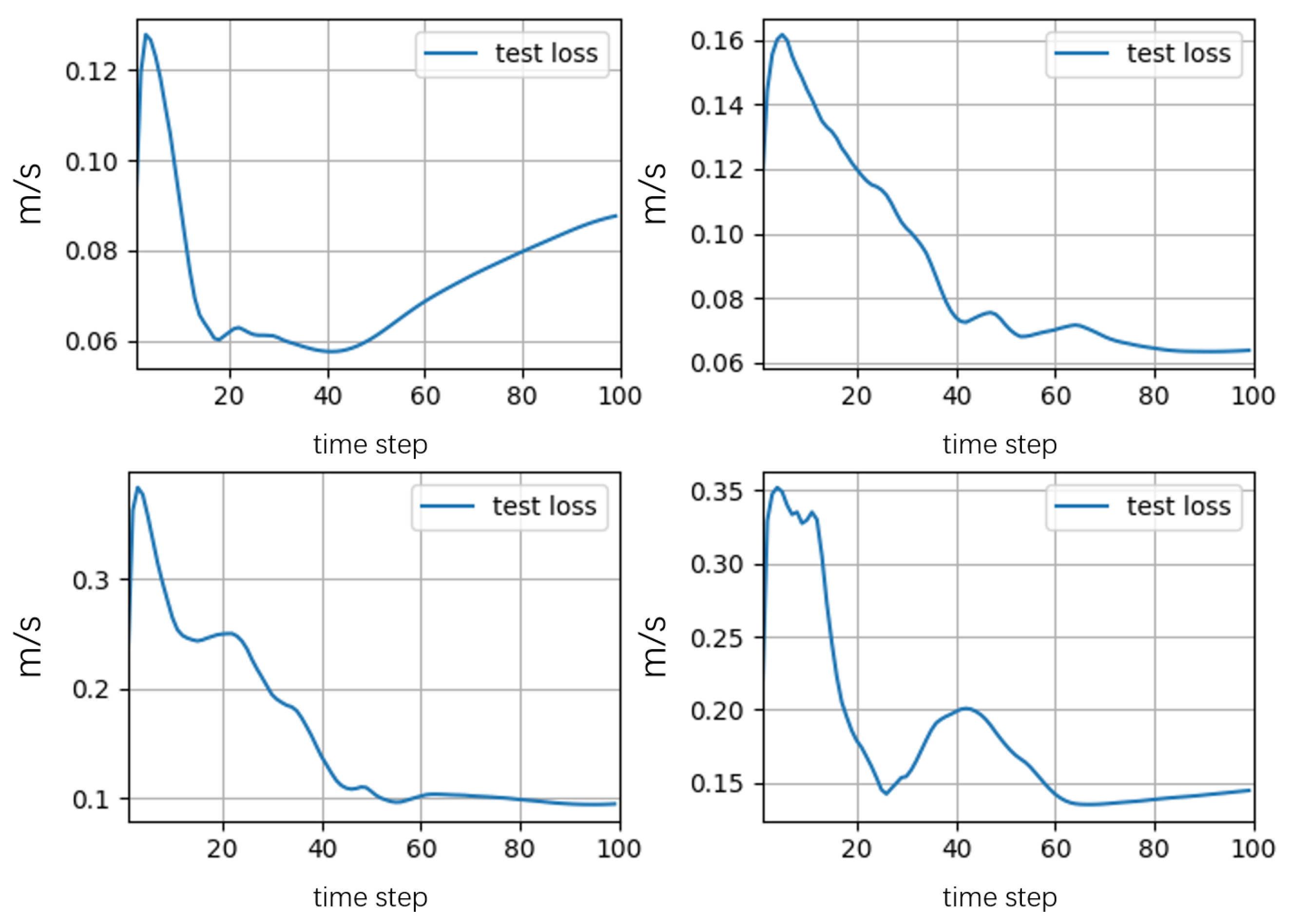
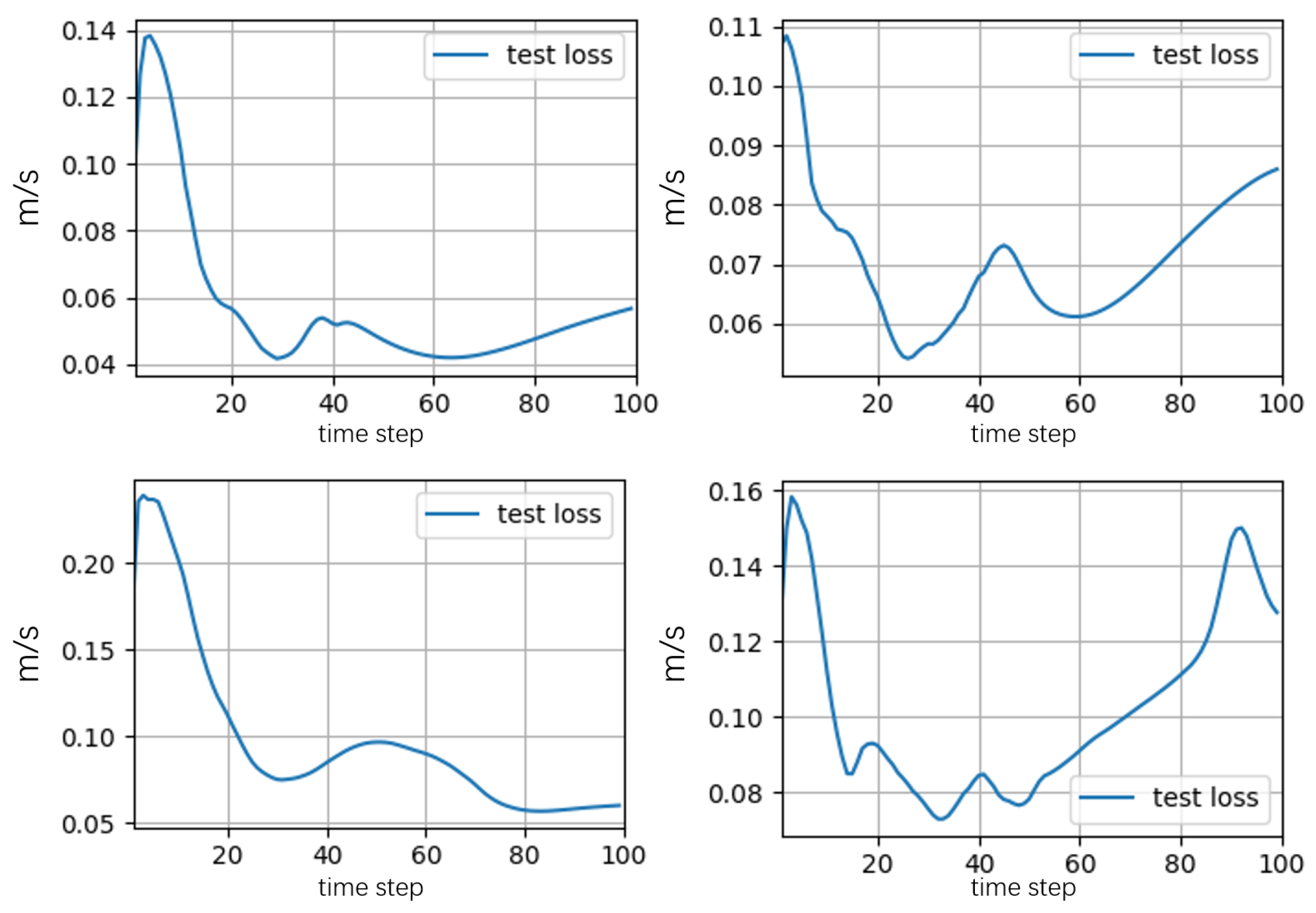
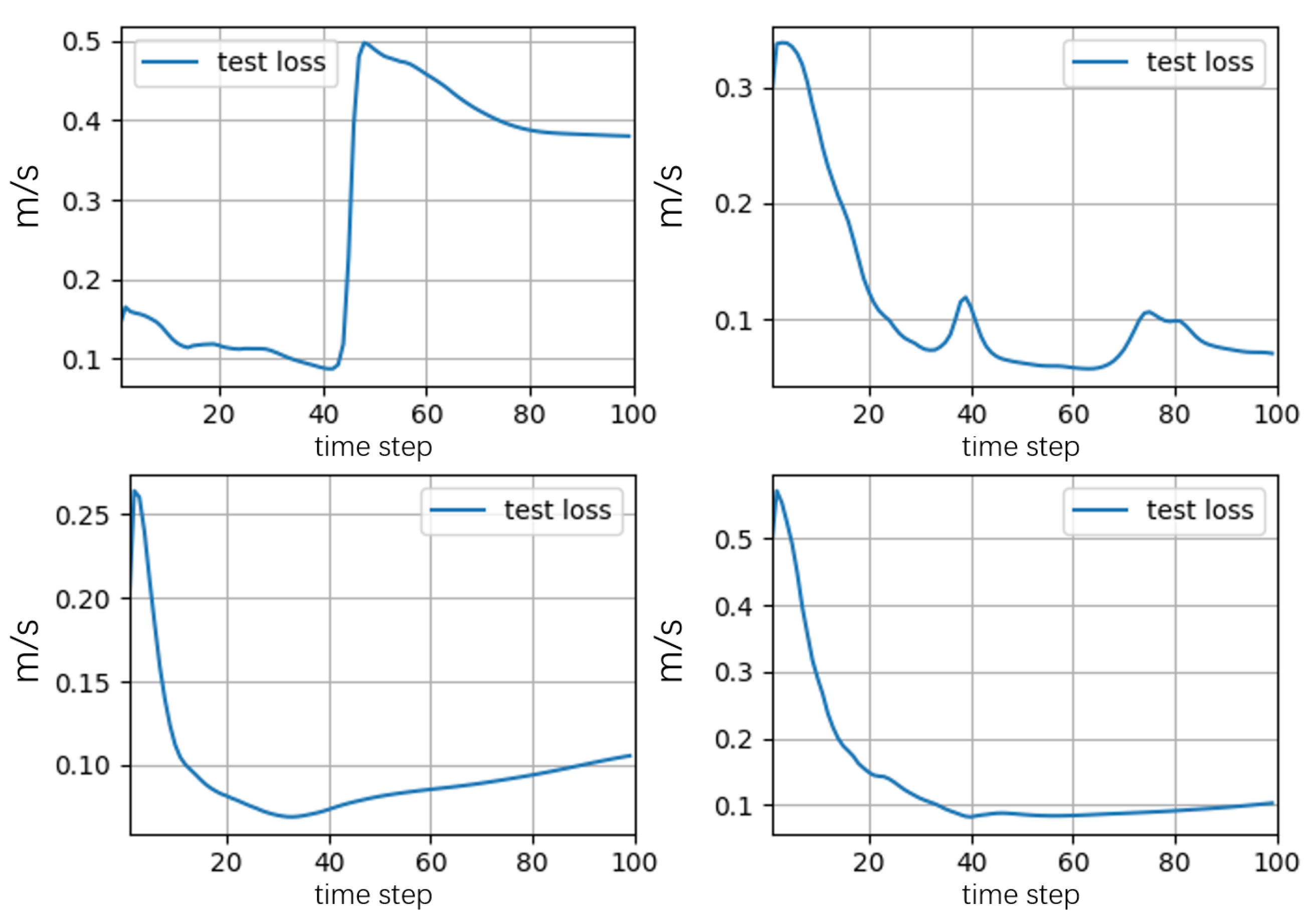
• Accuracy: Figure 6, Figure 7 and Figure 8 show the time evolution of the average velocity error (AVE) within each box compared to the monolithic SOWFA simulation of the two-turbine system on the test set.

  -

  Box 1 (upstream turbine): Similar to the single-turbine case, the AVE remained low, mostly below $0.2\mathrm{m}/\mathrm{s}$.

  -

  Box 2 (empty propagation): AVEs remained generally low, also mostly below $0.2\mathrm{m}/\mathrm{s}$, indicating that the ${\mathcal{M}}_{NN}^{NoWT}$ model effectively propagated the wake structure based on the inflow derived from Box 1’s NN prediction.

  -

  Box 3 (downstream turbine): AVEs were slightly higher than in Box 1 or 2, which is expected due to wake interaction and potential error accumulation through the stitching process. The AVEs generally stayed below $0.2\mathrm{m}/\mathrm{s}$ on average over the full rollout, with brief peaks during dynamic transitions. The average relative errors remained mostly within 2–5%, which is often considered acceptable for wake modeling applications.

  Overall, the stitched wind box model successfully captured the main dynamics of wake interaction, including the reduced velocity impinging on the downstream turbine, demonstrating the potential for this approach to model larger farm wake dynamics.
• Speed: Simulating the two-turbine 200 s scenario using the three stitched NN models took approximately 0.9–1.0 $\mathrm{s}$ on a V100 GPU (summing the inference time for each box). The corresponding monolithic SOWFA simulation took approximately $3\mathrm{h}30\min$ on a multi-core CPU (Intel Xeon E5-2680 v4, 2.4 GHz). The acceleration remains substantial (over 10,000×), demonstrating the computational efficiency of the wind box approach for extended farm layouts.

These results support the viability of the wind box decomposition strategy for building scalable and computationally efficient dynamic wake models for larger wind farms. While error accumulation at interfaces is a factor, the method provides a promising trade-off for applications requiring rapid prediction.

4.4. Discussion

The results demonstrate that the proposed data-driven surrogate modeling framework, combining a physics-inspired NN architecture with a scalable wind box strategy, can achieve a desirable balance between accuracy and computational speed for dynamic wind farm wake prediction. The AE structure effectively handles the high-dimensional spatial data by compressing it to a low-dimensional latent space, while the latent dynamics model efficiently captures the temporal evolution within this compressed representation. The wind box approach successfully scales the method to multiple turbines by decomposing the problem, significantly reducing the data generation burden and enabling the simulation of larger layouts than feasible with monolithic models. The inspiration drawn from the time–space structure of the N–S equations guided the architectural design towards decoupling spatial feature extraction and temporal evolution, which appears to be an effective inductive bias for this fluid dynamics problem. The computational time comparison of different models is shown in

Table 3. Comparison of simulation times for a 200 s physical duration (approximate).

Scenario	SOWFA (CFD) Time	NN Surrogate Time	Acceleration Factor
Single turbine (Case 1)	∼ 1 h 46 min	0.4–0.5 s	>10,000×
Two turbines (Case 2)	∼ 3 h 30 min	0.9–1.0 s	>10,000×
Analytical (e.g., FLORIDyn) *	N/A	∼2–3 s	N/A

* Note: FLORIDyn time is included for context from existing literature; it represents a different class of model (analytical/engineering) which is inherently faster but typically less accurate for complex 3D dynamic behavior than CFD or CFD-trained surrogates. NN surrogate times exclude model loading. The NN training time for each box model is significant (hours to days), but is amortized over many rapid inference runs.

.

The acceleration factor of over $10,000\times$ compared to SOWFA makes this approach highly promising for applications requiring rapid simulations, such as model predictive control, real-time optimization, and extensive layout studies, where CFD is currently impractical. The multi-objective training loss, including the latent space regularization $L_{ls}$, appears to contribute to learning stable and predictable dynamics in the compressed space by encouraging smoother latent space trajectories, indirectly promoting behavior analogous to the temporal integration of dynamics.

While effective for the tested two-turbine case, the observed slight increase in error in downstream boxes highlights the challenge of error propagation through the stitching process. The method for transferring boundary information between boxes is crucial. The current approach of sampling velocity planes provides detailed spatial context via a relatively high-dimensional input to the latent dynamics model. While this proved functional, further refinement could potentially improve accuracy and stability in longer wake chains or more complex multi-directional wake interactions. More sophisticated methods like using overlapping domains or dedicated interface correction NNs could be explored in future work to potentially improve the accuracy and stability of the boundary condition transfer. The sensitivity analysis of wind box size and placement is also a valuable direction for future work. The computational cost of training, while significant (in the order of hours to days for each box model depending on dataset size and complexity), is a one-time cost that is amortized over many rapid inference runs. Comparing the performance specifically to other *data-driven* surrogate models for 3D dynamic wake prediction is challenging due to the limited publicly available benchmarks for this specific problem class and resolution, but the demonstrated scalability via decomposition and the ability to capture detailed 3D dynamic fields represent key advancements compared to methods restricted to 2D or static analyses.

A highly relevant recent work by Wang et al. (2024) [44] also addresses dynamic wake field reconstruction using Physics-Informed Neural Networks (PINNs). Their method combines sparse LiDAR measurement data with the Navier–Stokes equations to reconstruct 3D dynamic wake fields, focusing on the influence of active yaw operation. They report RMSE values for velocity magnitude, with their PINN model consistently maintaining a low error level, typically below 0.24 m/s (less than 3 percent of free-stream velocity), even with varying scanning angle intervals and noise levels (see Figure 12 in [44]). This is notably accurate and demonstrates the power of physics-informed approaches for wake reconstruction.

• Data source and problem formulation: Wang et al. [44] primarily focus on **reconstructing** the wake field from *sparse LiDAR measurement data*, effectively solving an inverse problem constrained by PDEs. Our work, conversely, focuses on **predicting** the future 3D flow field in a *time-stepping manner* given a full initial state, using high-fidelity SOWFA (LES) data as ground truth. This is a crucial distinction: reconstruction (inferring the current state from sparse observations) and prediction (forecasting future states) serve different purposes and have different computational characteristics for continuous operation.
• Scalability to large wind farms: Our proposed “wind box” decomposition strategy is specifically designed to address the scalability challenge for **large wind farms** by breaking down the complex domain into smaller, canonical boxes that can be stitched together. This modularity allows for modeling arbitrary layouts without re-training a monolithic model for each new configuration, a challenge not explicitly addressed by reconstruction-focused PINNs like [44] which typically operate on a single, fixed-size subdomain around a turbine.
• Computational efficiency for long rollouts: Our NN surrogate model achieves a acceleration factor of over 10,000× for multi-time step *predictions* (reducing simulation times from hours to seconds). While PINNs are generally more efficient than full CFD, their computational cost for dynamic *prediction* over long time horizons, especially for high-resolution 3D turbulent flows with full PDE constraints, can still be substantial compared to our compact latent dynamics approach. The “time-stepping” nature of our model, facilitated by the autoencoder and latent dynamics, is highly efficient for multi-step rollouts, which is critical for real-time control applications.

This qualitative assessment highlights that, while there is growing synergy between deep learning and fluid dynamics for wind farm applications, our framework uniquely addresses the combination of high-fidelity 3D dynamic prediction with **unprecedented scalability and computational efficiency for continuous time-stepping simulation of large-scale wind farm layouts**, which complements and extends capabilities demonstrated by other cutting-edge data-driven approaches like PINN-based reconstruction.

5. Conclusions and Future Work

This paper addresses the critical need for fast and accurate 3D dynamic wake prediction models in wind farms, a long-standing challenge for layout optimization and operational control. To bridge the gap between slow high-fidelity CFD simulations and less detailed analytical or global data-driven models, we proposed a novel data-driven surrogate modeling framework built upon three core contributions. First, a unique physics-inspired neural network (NN) architecture was introduced, leveraging an autoencoder to compress high-dimensional 3D flow fields into a low-dimensional latent space, where a dedicated model learns the dynamic evolution, thereby effectively managing data dimensionality and aligning with fluid flow physics. Second, to overcome scalability limitations, a “wind box” methodology was developed, decomposing large wind farms into canonical smaller sub-domains (containing a single turbine or an empty wake region), with independent NN models trained for these standardized boxes then dynamically stitched together to simulate arbitrary and extensive farm layouts, drastically reducing the need for new, costly, full-farm CFD simulations. Third, a robust, automated SOWFA batch simulation and data processing toolchain was designed and implemented, crucial for systematically generating the high-fidelity 3D dynamic datasets required to efficiently train the surrogate models. The framework’s efficacy was rigorously validated against high-fidelity SOWFA simulations for both single-turbine and multi-turbine scenarios, consistently demonstrating high predictive accuracy (average velocity errors typically below 0.2 m/s, relative errors generally within 2–5% compared to SOWFA). Crucially, this high accuracy was achieved with unparalleled computational efficiency, with NN surrogate models delivering accelerations of over 10,000 times compared to SOWFA, reducing simulation times from hours to mere seconds, making the approach highly promising for real-time applications such as advanced wind farm control and rapid design optimization. In essence, this work presents a modular and physics-informed approach to learning fluid dynamics, specifically tailored for complex wind farm wakes, establishing a pathway towards enabling accurate, high-fidelity 3D dynamic wake predictions at a speed previously unattainable, thereby unlocking new possibilities for enhancing wind energy system efficiency and cost-effectiveness. Despite these promising results, future work should address limitations including the model’s dependence on the training data range for generalization, further optimizing the wind box interface handling to minimize error propagation, exploring more explicit physics-informed neural network (PINN) integrations, validating the approach on more realistic and complex wind farm conditions (e.g., terrain, atmospheric stability), and crucially, conducting rigorous comparisons with real-world wind farm measurement data.

References

- Xi, J. Keynote Speech at the Leaders’ Summit of the Fifteenth Meeting of the Conference of the Parties to the Convention on Biological Diversity (Full Text). Central People’s Government of China. Available online: https://www.gov.cn/xinwen/2021-10/12/content_5642048.htm (accessed on 12 October 2021).
- Xi, J. Speech During the Inspection Tour in Sichuan. Central People’s Government of the People’s Republic of China. Available online: https://www.gov.cn/yaowen/liebiao/202307/content_6895414.htm?device=app (accessed on 29 July 2023).
- China Wind Energy Committee, China Renewable Energy Society. 2023 China Wind Power Installation Capacity Statistical Brief; China Wind Energy Committee, China Renewable Energy Society: Beijing, China, 2024. [Google Scholar]
- National Energy Administration. 2023 National Power Industry Statistical Data; National Energy Administration: Beijing, China, 2024. Available online: https://www.gov.cn/lianbo/bumen/202401/content_6928723.htm (accessed on 28 January 2024).
- National Energy Administration. Modern Energy System Plan for the 14th Five-Year Period; National Energy Administration: Beijing, China, 2022.
- Sourkounis, C.; Tourou, P. Grid code requirements for wind power integration in europe. In Conference Papers in Science; Hindawi: London, UK, 2013; Volume 2013. [Google Scholar]
- National Technical Committee on Power Regulation Standardization. Technical Regulations for Wind Farm Connection to Power Systems [Standard]; China Standards Press: Beijing, China, 2011. [Google Scholar]
- Sichuan Economic and Information Technology Commission. Sichuan Automatic Generation Control Ancillary Service Market Trading Rules. n.d. Available online: http://www.escn.com.cn/news/show-738126.html (accessed on 17 May 2019).
- VanLuvanee, D.R. Investigation of Observed and Modeled Wake Effects at Horns rev Using Windpro; Technical University of Denmark, Department of Mechanical Engineering: Kongens Lyngby, Denmark, 2006. [Google Scholar]
- Zhao, L.; Gong, F.; Chen, S.; Wang, J.; Xue, L.; Xue, Y. Optimization study of control strategy for combined multi-wind turbines energy production and loads during wake effects. Energy Rep. 2022, 8, 1098–1107. [Google Scholar] [CrossRef]
- Hardy, S.; Ergun, H.; Van Hertem, D. A Greedy Algorithm for Optimizing Offshore Wind Transmission Topologies. IEEE Trans. Power Syst. 2022, 37, 2113–2121. [Google Scholar] [CrossRef]
- Ge, X.; Qian, J.; Fu, Y.; Lee, W.-J.; Mi, Y. Transient Stability Evaluation Criterion of Multi-Wind Farms Integrated Power System. IEEE Trans. Power Syst. 2022, 37, 3137–3140. [Google Scholar] [CrossRef]
- Peña, A.; Réthoré, P.-E.; van der Laan, M.P. On the application of the Jensen wake model using a turbulence-dependent wake decay coefficient: The Sexbierum case. Wind. Energy 2016, 19, 763–776. [Google Scholar] [CrossRef]
- Shen, Y.; Xiao, T.; Lv, Q.; Zhang, X.; Zhang, Y.; Wang, Y.; Wu, J. Coordinated optimal control of active power of wind farms considering wake effect. Energy Rep. 2022, 8, 84–90. [Google Scholar] [CrossRef]
- Tao, S.; Kuenzel, S.; Xu, Q.; Chen, Z. Optimal Micro-Siting of Wind Turbines in an Offshore Wind Farm Using Frandsen–Gaussian Wake Model. IEEE Trans. Power Syst. 2019, 34, 4944–4954. [Google Scholar] [CrossRef]
- Bastankhah, M.; Porté-Agel, F. A new analytical model for wind-turbine wakes. Renew. Energy 2014, 70, 116–123. [Google Scholar] [CrossRef]
- Gebraad, P.M.; Teeuwisse, F.; Van Wingerden, J.; Fleming, P.A.; Ruben, S.D.; Marden, J.R.; Pao, L.Y. Wind plant power optimization through yaw control using a parametric model for wake effects—A cfd simulation study. Wind Energy 2016, 19, 95–114. [Google Scholar] [CrossRef]
- Boersma, S.; Doekemeijer, B.M.; Gebraad, P.M.; Fleming, P.A.; Annoni, J.; Scholbrock, A.K.; Frederik, J.A.; van Wingerden, J.W. A tutorial on control-oriented modeling and control of wind farms. In Proceedings of the 2017 American Control Conference (ACC), Seattle, WA, USA, 24–26 May 2017; pp. 1–18. [Google Scholar]
- Chorin, J.A. Numerical solution of the Navier–Stokes equation. Math. Comput. 1968, 22, 745–762. [Google Scholar] [CrossRef]
- Deskos, G.; Piggott, M.D. Mesh-adaptive simulations of horizontal-axis turbine arrays using the actuator line method. Wind Energy 2018, 21, 1266–1281. [Google Scholar] [CrossRef]
- Han, Y.; Stoellinger, M.; Naughton, J. Large eddy simulation for atmospheric boundary layer flow over flat and complex terrains. J. Phys. Conf. Ser. 2016, 753, 032044. [Google Scholar] [CrossRef]
- Martínez-Tossas, L.A.; Churchfield, M.J.; Leonardi, S. Large eddy simulations of the flow past wind turbines: Actuator line and disk modeling. Wind Energy 2015, 18, 1047–1060. [Google Scholar] [CrossRef]
- Churchfield, M.; Lee, S.; Moriarty, P. Overview of the Simulator for Offshore Wind Farm Application (Sowfa) National Renewable Energy Laboratory; NREL/TP-5000-54704; NREL: Golden, CO, USA, 2012.
- von Rueden, L.; Mayer, S.; Sifa, R.; Bauckhage, C.; Garcke, J. Combining Machine Learning and Simulation to a Hybrid Modelling Approach: Current and Future Directions. In Advances in Intelligent Data Analysis XVIII; Berthold, M.R., Feelders, A., Krempl, G., Eds.; Springer International Publishing: Konstanz, Germany, 2020; pp. 548–560. [Google Scholar]
- Lavin, A.; Zenil, H.; Paige, B.; Krakauer, D.; Gottschlich, J.; Mattson, T.; Brehmer, J.; Anandkumar, A.; Choudry, S.; Rocki, K.; et al. Simulation Intelligence: Towards a New Generation of Scientific Methods. arXiv 2021, arXiv:2112.03235. [Google Scholar]
- Xiao, T.; Chen, Y.; Wang, J.; Huang, S.; Tong, W.; He, T. Exploration of Artificial Intelligence Oriented Power System Dynamic Simulators. J. Mod. Power Syst. Clean Energy 2022, 11, 401–411. [Google Scholar] [CrossRef]
- Bahaghighat, M.; Abedini, F.; Xin, Q.; Zanjireh, M.M.; Mirjalili, S. Using machine learning and computer vision to estimate the angular velocity of wind turbines in smart grids remotely. Energy Rep. 2021, 7, 8561–8576. [Google Scholar] [CrossRef]
- Marin, R.; Ciortan, S.; Rusu, E. A novel method based on artificial neural networks for selecting the most appropriate locations of the offshore wind farms. Energy Rep. 2022, 8, 408–413. [Google Scholar] [CrossRef]
- Ali, N.; Cal, R.B. Data-driven modeling of the wake behind a wind turbine array. J. Renew. Sustain. Energy 2020, 12, 033304. [Google Scholar] [CrossRef]
- Chen, K.; Lin, J.; Qiu, Y.; Liu, F.; Song, Y. Deep learning-aided model predictive control of wind farms for AGC considering the dynamic wake effect. Control Eng. Pract. 2021, 116, 104925. [Google Scholar] [CrossRef]
- Stevens, R.J.A.M.; Martinez-Tossas, L.A.; Meneveau, C. Large eddy simulation of the atmospheric boundary layer over a wind farm: Validation and sensitivity to the actuator disk model. J. Renew. Sustain. Energy 2016, 8, 154–168. [Google Scholar]
- Churchfield, M.J.; Lee, S.; Michaud, S.R.; NREL SOWFA Team. SOWFA: Simulating the Wind Farm Atmosphere; NREL/TP-5000-56093; 2012. Available online: https://www.nrel.gov/docs/libraries/wind-docs/sowfa-tutorial.pdf?sfvrsn=eb8c7763_1 (accessed on 20 June 2025).
- Cai, S.; Mao, Z.; Wang, Z.; Yin, M.; Em Karniadakis, G. Physics-informed neural networks (PINNs) for fluid mechanics: A review. Acta Mech. Sin. 2021, 37, 1727–1738. [Google Scholar] [CrossRef]
- Ali, M.; Cal, R.B. Deep learning for wind turbine wake estimation. Appl. Energy 2020, 269, 115042. [Google Scholar]
- Chen, T.; Qian, Z.; Chen, C.; Zhang, Y. A deep learning-based model predictive control for wind farm considering dynamic wake effects. Appl. Energy 2021, 300, 117392. [Google Scholar]
- Kim, J.; Lee, S. A review of machine learning applications in wind energy systems: A comprehensive overview. Energy Rep. 2021, 7, 7254–7278. [Google Scholar]
- Raissi, M.; Perdikaris, P.; Karniadakis, G.E. Physics-informed neural networks: A deep learning framework for solving forward and inverse problems involving nonlinear partial differential equations. J. Comput. Phys. 2019, 378, 686–707. [Google Scholar] [CrossRef]
- Raissi, M.; Perdikaris, P.; Karniadakis, G.E. Physics informed deep learning (part I): Data-driven solutions of nonlinear partial differential equations. arXiv 2017, arXiv:1711.10561. [Google Scholar]
- Liu, B.; Wang, Y.; Rabczuk, T.; Olofsson, T.; Lu, W. Multi-scale modeling in thermal conductivity of polyurethane incorporated with phase change materials using physics-informed neural networks. Renew. Energy 2024, 220, 119565. [Google Scholar] [CrossRef]
- Li, P.; Liu, M.; Alfarrla, M.; Tahmasebi, P.; Grana, D. Probabilistic physics-informed neural network for seismic petrophysical inversion. Geophysics 2024, 89, M17–M32. [Google Scholar] [CrossRef]
- Huang, B.; Wang, J. Applications of physics-informed neural networks in power systems-a review. IEEE Trans. Power Syst. 2022, 38, 572–588. [Google Scholar] [CrossRef]
- Stiasny, J.; Misyris, G.S.; Chatzivasileiadis, S. Transient stability analysis with physics-informed neural networks. arXiv 2021, arXiv:2106.13638. [Google Scholar]
- Daniele, L.-O.; Meanti, G.; Pagliana, N.; Verri, A.; Mazzino, A.; Rosasco, L.; Seminara, A. Physics informed machine learning for wind speed prediction. Energy 2023, 268, 126628. [Google Scholar]
- Wang, L.; Chen, M.; Luo, Z.; Zhang, B.; Xu, J.; Wang, Z.; Tan, Z.C.C. Dynamic wake field reconstruction of wind turbine through Physics-Informed Neural Network and Sparse LiDAR data. Energy 2024, 291, 130401. [Google Scholar] [CrossRef]
- Zhang, J.; Zhao, X. Digital twin of wind farms via physics-informed deep learning. Energy Convers. Manag. 2023, 293, 117507. [Google Scholar] [CrossRef]
- Xiao, T.; Cao, Y.; Liang, B.; Wang, Y.; Wang, J.; Chen, Y. Design and implementation of a general batch simulation tool of SOWFA and its application in training a single-turbine surrogate. Energy Rep. 2023, 9, 419–426. [Google Scholar] [CrossRef]