Modeling and Simulation Analysis of Three-Phase Saturable Transformers: A Study on the Effects of Geomagnetically Induced Current on Transformers

Abstract

The saturation model of the transformer is one of the core tools of multi-physics simulation. By combining it with multi-physics simulation, researchers can more comprehensively evaluate the performance of a transformer in actual applications. Geomagnetically induced currents (GIC) induce DC bias in transformers, leading to core saturation and a host of adverse effects. Traditional transformer models often struggle to accurately capture the behavior of the core under nonlinear saturation conditions. To address these challenges, a saturable transformer unified magnetic-equivalent (UMEC) model that directly takes the B-H magnetization curve to represent a transformer’s core nonlinear characteristics is proposed. The saturable transformer model is based on the model of a magnetic circuit of the transformer core. An estimation method to obtain a transformer’s essential parameters for saturation simulation is presented. GIC effects on transformer saturation are also studied through the proposed saturable transformer and estimation method.

1. Introduction

Transformers serve as crucial electrical equipment and play an essential role. As power demand keeps growing and the requirements for power system reliability are continuously rising, the accurate modeling and analysis of transformers are of particular significance [1]. Conceptually, the design of a transformer is relatively simple. However, with the presence of diverse types of magnetic cores and coil arrangements, along with the impact of magnetic saturation, the characterization of a transformer becomes highly complex. Moreover, this complexity significantly influences the transient properties of the transformer. It is also important to represent saturation effects in transformers for geomagnetically induced current (GIC) studies [2]. Relevant studies indicate that the transformer model in the transient simulation package is one of the components in greatest need of improvement [3,4].

Research on transformers focuses on two key aspects: describing the magnetic characteristics of the core and establishing the coupling relationship between electricity and magnetism. The main methods used to study the coupling relationship between the electrical circuit and the magnetic circuit of core materials include the finite element method (FEM) [5], the dual model [6], and the unified magnetic-equivalent circuit (UMEC) [7]. In [8,9], the impact of GIC on transformers with different structures is studied using magnetic circuit analysis and the FEM. These studies aim to contribute to the understanding of the fundamental transformer magnetization mechanism under GIC. In [10], based on the harmonic-balanced FEM, a hysteresis model for the loss function was established. This approach corrects the magnetization curve under DC bias conditions and analyzes the impact of DC bias on the iron core, considering hysteresis effects. Using the FEM to study transformer DC bias issues provides accurate results, but it involves a large computational scale and requires a significant amount of time.

The derivation of representative electromagnetic transients (EMT) transformer models, namely the dual model and the UMEC model, has been extensively researched to enhance accuracy for mid- to low-frequency studies. In [5,11], based on the circuit duality principle, researchers perform duality transformation on the electrical parameters and magnetic circuit parameters of the transformer to convert the magnetic circuit into an equivalent circuit. In [12], a new model and algorithm for solving nonlinear DC bias problems has been proposed. By using transformer magnetic–electric circuit coupling equations, the impact of DC bias on a three-phase five-limb transformer is analyzed. The dual model offers certain advantages in particular analysis scenarios, for instance, simplifying the analysis of complex systems. Nevertheless, its applicability in the case of nonlinearity and the special working conditions of transformers is relatively restricted.

In [13], a single-phase, four-limb converter transformer is studied, and a UMEC model calculation method based on no-load test data is proposed. This method accelerates the electromagnetic transient simulation speed. Large transformers usually adopt a three-phase, three-limb or three-phase, five-limb structure [14]. However, the magnetic circuit structure of this kind of transformer is very complex, and there is magnetic coupling between phases, which brings difficulties to the research on magnetic field and loss distribution. There are already saturable transformer models in commercial simulation software. The UMEC model in PSCAD uses a V-I curve to represent a nonlinear characteristic of the transformer core; however, this curve is normally only available to manufacturers [15]. The saturable transformer model in MATLAB/Simulink takes a three-single saturable transformer to represent a three-phase transformer; thus, it cannot accurately represent a three-phase, three-leg or five-leg transformer [16]. In [17], based on the analysis of the B-H curve of the magnetic core and magnetizing current, an efficient method for modeling the global magnetic properties of the transformer under DC-biased conditions is proposed. However, the existing property data of the magnetic material provided by the manufacturer are usually not sufficient. Regarding the validation of the UMEC model, advanced saturation sensing techniques, such as high-frequency sensing [18], power loss sensing [19], and electrical parameter sensing [20], provide a way to collect real-time and accurate data about the magnetic state of inductors. In this paper, a saturable UMEC transformer model within the MATLAB/Simulink framework, which incorporates a B-H magnetization curve, is employed. The modeling approach is guided by the aim of finding a transformer model whose data is easy to get, and the model should be accurate to represent a three-phase, three-leg or five-leg transformer.

The remainder of the paper is organized as follows: In Section 2, an estimation method for transformer core dimensions and winding parameters is discussed. Based on this estimation method, the saturable UMEC transformer model is discussed in Section 3. In Section 4, the validity and accuracy of the model were verified through case testing. A test case to study the GIC effect on the transformer is carried out, and a detailed analysis is presented in Section 5. In Section 6, a summary is drawn.

2. Materials and Methods

The transformer parameter estimation method aims to obtain essential data to supply these data for the saturable transformer model. An optimized transformer design procedure is complicated and time-consuming, constituting professional knowledge for transformer manufacturers. For power system researchers and transmission system operators (TSOs), it is not necessary to concentrate on detailed transformer parameters, such as structure parts’ arrangement and wingding arrangements. The transformer parameter estimation method proposed in this document is worked out using easily available data to estimate essential data, i.e., core dimensions and winding turns, for power system simulation purposes.

Some values, such as no-load current and no-load power factor, should be given, which represent dependency between core structure and exciting current values. Using some reasonable assumptions and easily available values, the estimation method presented in this document can work out the essential transformer parameters for the saturable transformer model.

2.1. Available Data for Estimation

This section introduces the input data that are necessary for the estimation of a three-phase, three-winding, large power transformer. The transformer windings are made of copper. The input data are split into two categories, as described in the following tables.

Table 1. System parameters of three-phase, three-winding transformer.

Symbol	Quantity	Unit
SHV	Capacity of high-voltage side	kVA
SMV	Capacity of medium-voltage side	kVA
SLV	Capacity of low-voltage side	kVA
UHV	Line-to-line voltage of high-voltage side	kV
UMV	Line-to-line voltage of medium-voltage side	kV
ULV	Line-to-line voltage of low-voltage side	kV
f	Frequency	Hz

describes system parameters that are easily obtained.

Table 2. Desired no-load operation characteristics.

Symbol	Quantity	Unit
Br	Magnetic flux density	T
Ino-load	RMS of no-load current	A
cos(φ0)	No-load power factor	T

describes some desired no-load operation characteristics that are closely related to the transformer structure.

For an oil-filled electric transformer, B is reasonable between 1.58 T and 1.72 T. For the same transformer, a larger magnetic flux density reduces manufacturing costs at the expense of lowering the overexciting capability. No-load current and power factor are closely related through a compromise between winding copper and core electrical steel. These data can be easily obtained. To estimate transformer parameters, some reasonable assumptions should be made here [21,22]: (1) the length of the yoke and main leg is the same; (2) leakage inductance is much lower than excitation inductances and is, therefore, neglected in the estimation of transformer parameters; and (3) magnetic flux in three main legs is symmetrical at the no-load unsaturated condition.

2.2. Calculation Process

In this section, a detailed estimation process of transformer parameters will be discussed. The calculation processes for three-leg and five-leg transformers are the same, except that the five-leg transformer has a side leg and yoke with different cross-sectional areas. In the following calculation steps, a general process will be given.

2.2.1. Calculation of Turns

The voltage per turn is closely related to the types of transformers, winding arrangement insulation, and requirements. One relationship embodying such experience is as follows [23]:

$$V_{\mathrm{t}}={\displaystyle \frac{\sqrt{S}}{C}}, 20 < C < 70$$

(1)

where $V_{\mathrm{t}}$ is the voltage per turn at the high-voltage side, S is the apparent power, and C is the experimental factor, which depends on the type of construction and intended service of the transformer.

Winding turns at high-voltage side are obtained as follows:

$$N_{\mathrm{HV}}={\displaystyle \frac{U_{\mathrm{HV}}}{V_{\mathrm{t}}}}$$

(2)

where $N_{\mathrm{HV}}$ is the turns at the high-voltage side, and $U_{\mathrm{HV}}$ is the rated voltage at the high-voltage side.

Winding turns at the medium- and low-voltage sides are obtained from the voltage ratio:

$$N_{\mathrm{MV}}={\displaystyle \frac{N_{\mathrm{HV}}{U}_{\mathrm{MV}}}{U_{\mathrm{HV}}}}$$

(3)

$$N_{\mathrm{LV}}=N_{\mathrm{HV}}\cdot {\displaystyle \frac{U_{\mathrm{LV}}}{U_{\mathrm{HV}}/\sqrt{3}}}$$

(4)

2.2.2. Calculation of Main Leg Cross Section

The voltage source applied at the transformer winding terminal is as follows:

$$\left\{\begin{array}{l}{u}_{\mathrm{a}}={\displaystyle \frac{U_{\mathrm{HV}}}{\sqrt{3}}}\sqrt{2}\cos (\omega t)\\ u_{\mathrm{b}}={\displaystyle \frac{U_{\mathrm{HV}}}{\sqrt{3}}}\sqrt{2}\cos (\omega t-120)\\ u_{\mathrm{c}}={\displaystyle \frac{U_{\mathrm{HV}}}{\sqrt{3}}}\sqrt{2}\cos (\omega t+120)\end{array}\right.$$

(5)

As we have assumed in previous sections, the induced electromotive force is as follows:

$$\left\{\begin{array}{l}{e}_{\mathrm{a}}={\displaystyle \frac{U_{\mathrm{HV}}}{\sqrt{3}}}\sqrt{2}\cos (\omega t)\\ e_{\mathrm{b}}={\displaystyle \frac{U_{\mathrm{HV}}}{\sqrt{3}}}\sqrt{2}\cos (\omega t-120)\\ e_{\mathrm{c}}={\displaystyle \frac{U_{\mathrm{HV}}}{\sqrt{3}}}\sqrt{2}\cos (\omega t+120)\end{array}\right.$$

(6)

According to $e_{\mathrm{a}}=N_{\mathrm{HV}}{\displaystyle \frac{\mathrm{d}{\Phi }_{\mathrm{a}}}{\mathrm{d}t}}$:

$${\Phi }_{\mathrm{a}}={\displaystyle \frac{1}{N_{\mathrm{HV}}}}{\displaystyle \int e_{\mathrm{a}}}\mathrm{d}t={\displaystyle \frac{\sqrt{2}{U}_{\mathrm{HV}}}{\sqrt{3}{N}_{\mathrm{HV}}\omega }}\sin (\omega t)+{\Phi }_0$$

(7)

where ${\Phi }_{\mathrm{a}}$ is the magnetic flux in phase A, ${\Phi }_0$ is the DC magnetic flux, $N_{\mathrm{HV}}$ is the number of turns at the high-voltage side, and $\omega$ is the angular velocity.

At a steady state without a DC flux bias,

$${\Phi }_0=0$$

(8)

This estimation method takes symmetrical flux in three main legs into consideration. Magnetic flux in three main legs cannot be exactly symmetrical due to the asymmetrical flux path. For transformer design, the assumption of symmetrical fluxes in the main legs is reasonable and acceptable.

According to Equation (7), the maximum magnetic flux is as follows:

$${\Phi }_{\max }={\displaystyle \frac{\sqrt{2}{U}_{\mathrm{HV}}}{\sqrt{3}{N}_{\mathrm{HV}}\omega }}$$

(9)

The maximum magnetic flux density at no-load unsaturated conditions is as follows:

$${\Phi }_{\max }=B_{\max }\times A_{\mathrm{ml}}$$

(10)

According to Equations (9) and (10), the cross section of the main leg is as follows:

$$A_{\mathrm{ml}}={\displaystyle \frac{\sqrt{2}{U}_{\mathrm{HV}}}{\sqrt{3}{N}_{\mathrm{HV}}\omega B_{\max }}}$$

(11)

2.2.3. Calculation of Magnetic Flux Density and Magnetic Field Strength

Assume that the magnetic flux in the main legs is symmetrical; then, the values are as follows:

$$\left\{\begin{array}{l}{\Phi }_{\mathrm{a}}={\Phi }_{\mathrm{r}}\sin (\omega t)\\ {\Phi }_{\mathrm{b}}={\Phi }_{\mathrm{r}}\sin (\omega t-120)\\ {\Phi }_{\mathrm{c}}={\Phi }_{\mathrm{r}}\sin (\omega t+120)\end{array}\right.$$

(12)

As we have discussed in previous sections, the magnetic flux in phase A gets to its maximum value, $\omega t=\pi /2$. Inserting $\omega t=\pi /2$ into (12) leads to the following:

$$\left\{\begin{array}{l}{\Phi }_{\mathrm{a}1}={\Phi }_{\mathrm{r}}\\ {\Phi }_{\mathrm{b}1}=-0.5{\Phi }_{\mathrm{r}}\\ {\Phi }_{\mathrm{c}1}=-0.5{\Phi }_{\mathrm{r}}\end{array}\right.$$

(13)

According to $\Phi ={\rm B}\times A$,

$$\left\{\begin{array}{l}{B}_{\mathrm{a}1}={\displaystyle \frac{{\Phi }_{\mathrm{a}1}}{A_{\mathrm{m}1}}}\\ B_{\mathrm{b}1}={\displaystyle \frac{{\Phi }_{\mathrm{b}1}}{A_{\mathrm{m}1}}}\\ B_{\mathrm{c}1}={\displaystyle \frac{{\Phi }_{\mathrm{c}1}}{A_{\mathrm{m}1}}}\end{array}\right.$$

(14)

2.2.4. Calculation of No-Load Excitation Current

The no-load exciting current is closely related to transformer dimensions and is essential to this estimation method. The no-load exciting current can be obtained from the no-load test on the physical transformer. If test data are not easy to get, researchers can assume a reasonable value. As we have assumed in the assumptions section, the no-load current and no-load power factor are known. The no-load current in phase A can be calculated as follows:

$$i_{\mathrm{a}}=I_{\mathrm{no-load}}\cdot \sqrt{2}\cos (\omega t+{\phi }_0)$$

(15)

At $\omega t={\displaystyle \frac{\pi }{2}}$, the instantaneous exciting current in phase A can be calculated as follows:

$$i_{\mathrm{a}}=I_{\mathrm{no-load}}\cdot \sqrt{2}\cos ({\displaystyle \frac{\pi }{2}}+{\phi }_0)$$

(16)

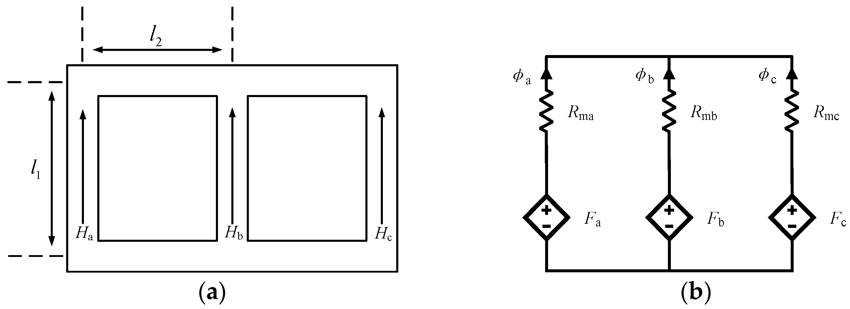
2.2.5. Calculation of Lengths of Leg and Yoke

To calculate the lengths of the leg and yoke, a three-leg transformer is adopted here because of its fewer unknown variables. The core dimensions and its magnetic circuit can be seen in Figure 1. For the notation, $l_1$ is the length of the main leg, $l_2$ is the length of the yoke, $H_{\mathrm{a},\mathrm{b},\mathrm{c}}$ is the magnetic field strength in phase A, B, and C, $F_{\mathrm{a},\mathrm{b},\mathrm{c}}$ is the magnetomotive force in phase A, B, and C, and $R_{\mathrm{ma},\mathrm{mb},\mathrm{mc}}$ is the reluctance.

According to the magnetic circuit in Figure 1, we can obtain equations as follows:

$$\left\{\begin{array}{l}{F}_{\mathrm{a}1}-F_{\mathrm{c}1}={\Phi }_{\mathrm{a}1}\cdot R_{\mathrm{ma}}-{\Phi }_{\mathrm{c}1}\cdot R_{\mathrm{mc}}\\ F_{\mathrm{b}1}-F_{\mathrm{c}1}={\Phi }_{\mathrm{b}1}\cdot R_{\mathrm{mb}}-{\Phi }_{\mathrm{c}1}\cdot R_{\mathrm{mc}}\end{array}\right.$$

(17)

Large power transformers are often not grounded, which leads to the following:

$$i_{\mathrm{a}1}+i_{\mathrm{b}1}+i_{\mathrm{c}1}=0$$

(18)

According to Maxwell’s equation,

$${\displaystyle {\sum }_i}{N}_i{I}_i={\displaystyle \oint H\mathrm{d}l}$$

(19)

Equations (17) and (18) can be written as follows:

$$\left\{\begin{array}{l}2N_{\mathrm{HV}}\cdot i_{\mathrm{a}1}+N_{\mathrm{HV}}\cdot i_{\mathrm{b}1}=H_{\mathrm{a}1}\cdot (2l_2+l_1)-H_{\mathrm{c}1}\cdot (2l_2+l_1)\\ 2N_{\mathrm{HV}}\cdot i_{\mathrm{b}1}+N_{\mathrm{HV}}\cdot i_{\mathrm{a}1}=H_{\mathrm{b}1}\cdot l_1-H_{\mathrm{c}1}\cdot (2l_2+l_1)\end{array}\right.$$

(20)

In (20), there are three unknown parameters: $l_1$, $l_2$, and $i_{\mathrm{b}}$. As we have discussed in the assumption section, $l_1=l_2$. Solving (20), we can get the value of $l_1$ and $l_2$:

$$l_1=l_2={\displaystyle \frac{3N{i}_{\mathrm{a}1}}{6H_{\mathrm{a}1}-H_{\mathrm{b}1}-3H_{\mathrm{c}1}}}$$

(21)

2.2.6. Calculation of Yoke and Side-Leg Cross Section

The main leg dimensions and winding turns are the same for three-leg and five-leg transformers, while the yoke and side-leg cross sections of three-leg and five-leg transformers are different. For a three-leg transformer, the cross section of the leg and yoke should have the same area because there is the same flux in the leg and the corresponding yoke. The cross-sectional area of the yoke can be calculated as follows:

$$A_{\mathrm{yo}}=A_{\mathrm{ml}}$$

(22)

For large power transformers, it is often necessary to lower the transformer height due to transportation limitations. The application of a five-leg core in a three-phase transformer allows for reducing the section of yokes to about $\sqrt{3}/3$ of the yoke section in a typical three-leg core while maintaining full transformer power and unchanged dimensions for the main legs [24]. According to the data sheet from ABB, an approximate equation is adopted for transformer design as follows:

$$\left\{\begin{array}{l}{A}_{\mathrm{yo}}={\displaystyle \frac{\sqrt{3}}{3}}{A}_{\mathrm{ml}}\\ A_{\mathrm{sl}}={\displaystyle \frac{1}{2}}{A}_{\mathrm{ml}}\end{array}\right.$$

(23)

3. Modeling of Saturation in Three-Phase Transformer

The UMEC model considers magnetic coupling between windings of different phases, in addition to coupling between windings of the same phase. The UMEC model requires the user to input an accurate nonlinear voltage–current curve. Within the transformer core material, this nonlinear relationship is conspicuously exhibited. With the augmentation of the input current, the resultant magnetic field strength becomes enhanced. The magnetic flux density within the core ascends rapidly during the initial phase. Nevertheless, upon nearing saturation, even if the magnetic field strength persists in increasing, the rate of increase in the magnetic flux density becomes minimal. In the design and operation analysis model of power transformers, if the nonlinear variation between magnetic flux density and magnetic field strength during core saturation cannot be accurately represented, it may lead to incorrect estimations of crucial performance indicators such as voltage regulation characteristics, loss calculations, and short-circuit impedance of the transformer. Consequently, this would affect the optimal design and safe operation of the transformer, as well as its matching and coordination with other equipment in the power system.

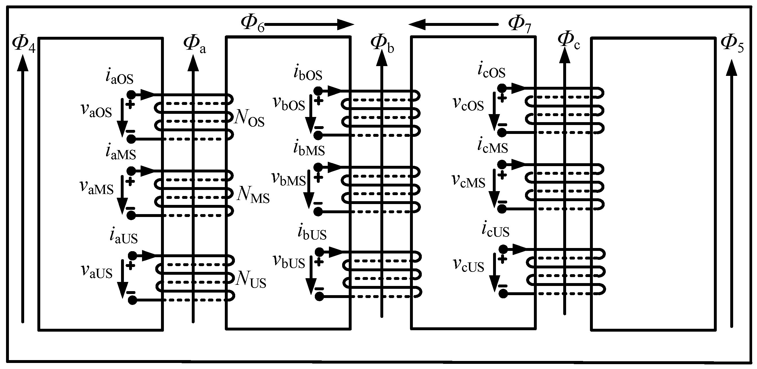
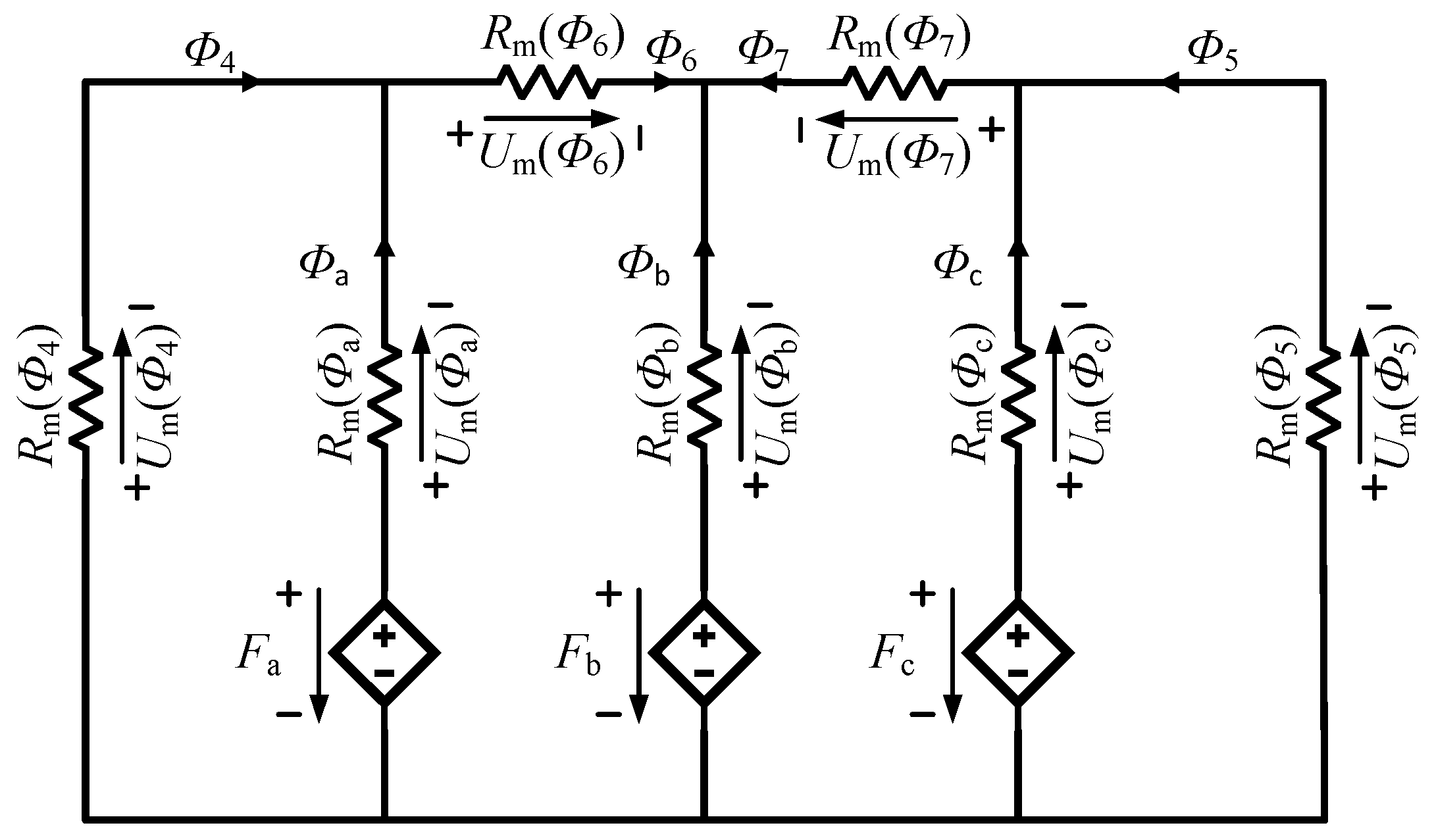
Building upon the foundational UMEC model, a saturable transformer model based on a physical model is proposed in this section. This model considers specific B-H saturation characteristics, detailed core dimensions, and winding turns. The detailed structure of the three-phase, three-winding, five-leg core transformer is shown in Figure 2. The associated UMEC model of a three-phase, three-winding, five-leg core transformer is shown in Figure 3. For the notation, F is the magnetic force, $R_{\mathrm{m}}$ is the reluctance, $U_{\mathrm{m}}$ is the magnetic force drops on reluctance, j is the subscript that denotes parts of the transformer core, and v is the subscript that denotes phase a, b, or c.

Two approximations in the magnetic circuit are introduced: (1) the reluctances in all parts of the transformer core, i.e., the main leg, side leg, and yoke, are assumed to be described by the same function, $R_{\mathrm{m}}({\Phi }_j)$; and (2) the leakage magnetic flux in the air is neglected. The winding voltage $e_v$ is related to branch flux ${\Phi }_v$ through the following:

$$e_v=N_v{\displaystyle \frac{\mathrm{d}{\Phi }_v}{\mathrm{d}t}}$$

(24)

where $e_v$ is the induced electromotive force at the winding terminal.

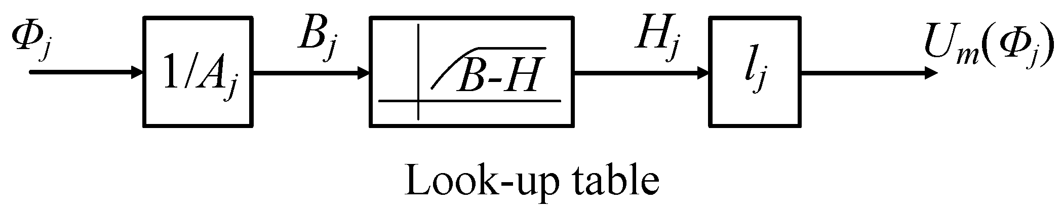
The nonlinear permeance is represented in Figure 4. For the notation, $A_j$ is the cross area of branch j in the transformer core; $l_j$ is the length of branch j in the transformer core.

The magnetic flux ${\Phi }_j$ in part j of the transformer core is obtained from the magnetic circuit in Figure 3. The magnetic flux in the main leg can be deduced from Equation (24).

The flux in each branch can be written in vector form as follows:

$$\mathit{\Phi }=\mathit{P}(\mathit{N}\mathit{I}-{\mathit{U}}_{\mathbf{m}})$$

(25)

where $\mathit{P}$ is the permeance matrix. It is governed by the magnetic permeability of the core material, as well as the physical parameters of the core. $\mathit{N}$ is the winding turns matrix (zero for branches without winding), $\mathit{I}$ is the vector of winding current (zero for branches without winding), and ${\mathit{U}}_{\mathbf{m}}$ is the vector of magnetomotive drop in each branch.

The flux must sum to zero at each UMEC node, which can be described as follows:

$${\mathit{A}}^{\mathbf{T}}\mathit{\Phi }=\mathbf{0}$$

(26)

where $\mathit{A}$ is the connection matrix of the magnetic circuit. In the magnetic circuit analysis of a transformer, the magnetic circuit connection matrix A is used to describe the connection relationships among various parts in the magnetic circuit system. The most basic elements are 0 and 1, which represent the connection status. If the number of UMEC branches is m, the number of nodes is n, and then $\mathit{A}$ is the $m\times n$ rectangular branch connection matrix.

Applying connection matrix $\mathit{A}$ to the vector of nodal m.m.f gives the branch m.m.f:

$$\mathit{A}{\mathit{U}}_{\mathbf{mnode}}={\mathit{U}}_{\mathbf{m}}$$

(27)

where ${\mathit{U}}_{\mathbf{mnode}}$ is the vector of nodal m.m.f at each node.

Combining (24)–(26) gives the following:

$$\mathit{f}=\mathit{Q}\mathit{P}\mathit{N}\mathit{I}$$

(28)

with

$$\mathit{Q}=\mathit{E}-\mathit{P}\mathit{A}{({\mathit{A}}^{\mathbf{T}}\mathit{P}\mathit{A})}^{-1}{\mathit{A}}^{\mathbf{T}}$$

(29)

where $\mathit{P}$ is the $m\times m$ diagonal matrix of branch permeances. $\mathit{E}$ is the $m\times m$ diagonal identity matrix.

The application of the trapezoidal integration method to (24) gives the following:

$${\mathit{f}}_{\mathrm{s}}(t)={\mathit{f}}_{\mathrm{s}}(t-\Delta t)+{\displaystyle \frac{\Delta t}{2}}{{\mathit{N}}_{\mathrm{s}}}^{-1}({\mathit{V}}_{\mathrm{s}}(t)+{\mathit{V}}_{\mathrm{s}}(t-\Delta t))$$

(30)

where ${\mathit{f}}_{\mathrm{s}}$ is the $n\times 1$ matrix of magnetic flux in the main leg, ${\mathit{N}}_{\mathrm{s}}$ is the $n\times n$ diagonal matrix of the winding turns’ number, and $\Delta t$ is the time-step size.

Eventually, the winding current can be obtained from the Norton equivalent [25]:

$${\mathit{i}}_{\mathrm{s}}(t)={\mathit{Y}}_{\mathrm{ss}}{\mathit{V}}_{\mathrm{s}}(t)+{\mathit{i}}_{\mathrm{ns}}(t)$$

(31)

with

$${\mathit{Y}}_{\mathrm{SS}}={\mathit{Q}}_{\mathrm{SS}}{\mathit{P}}_{\mathrm{SS}}{\mathit{N}}_{\mathrm{S}}^{-1}{\displaystyle \frac{\Delta t}{2}}{{\mathit{N}}_{\mathrm{s}}}^{-1}$$

(32)

$${\mathit{i}}_{\mathrm{ns}}(t)=({\mathit{Q}}_{\mathrm{SS}}{\mathit{P}}_{\mathrm{SS}}{\mathit{N}}_{\mathrm{S}})({\displaystyle \frac{\Delta t}{2}}{{\mathit{N}}_{\mathrm{s}}}^{-1}{\mathit{V}}_{\mathrm{s}}(t-\Delta t)+{\mathit{f}}_{\mathrm{s}}(t-\Delta t)){\mathit{Y}}_{\mathrm{SS}}={\mathit{Q}}_{\mathrm{SS}}{\mathit{P}}_{\mathrm{SS}}{\mathit{N}}_{\mathrm{S}}^{-1}{\displaystyle \frac{\Delta t}{2}}{{\mathit{N}}_{\mathrm{s}}}^{-1}$$

(33)

where ${\mathit{Q}}_{\mathrm{SS}}$ is the upper left-hand partition of the matrix $\mathit{Q}$ in Equations (26)–(29). ${\mathit{P}}_{\mathrm{SS}}$ is the $n\times n$ upper left-hand partition of matrix $\mathit{P}$.

For the UMEC in Figure 2 and Figure 3, it can be expressed as the Norton equivalent circuit. Equations (26)–(31) becomes the following:

$$\left(\begin{array}{l}{i}_{\mathrm{aOS}}(t)\\ i_{\mathrm{aMS}}(t)\\ i_{\mathrm{aTS}}(t)\\ i_{\mathrm{bOS}}(t)\\ i_{\mathrm{bMS}}(t)\\ i_{\mathrm{bTS}}(t)\\ i_{\mathrm{cOS}}(t)\\ i_{\mathrm{cMS}}(t)\\ i_{\mathrm{cTS}}(t)\end{array}\right)=\left(\begin{array}{ccccccccc}{y}_{11}& y_{12}& y_{13}& y_{14}& y_{15}& y_{16}& y_{17}& y_{18}& y_{19}\\ y_{21}& y_{22}& y_{23}& y_{24}& y_{25}& y_{26}& y_{27}& y_{28}& y_{29}\\ {\mathrm{y}}_{31}& {\mathrm{y}}_{32}& {\mathrm{y}}_{33}& {\mathrm{y}}_{34}& {\mathrm{y}}_{35}& {\mathrm{y}}_{36}& {\mathrm{y}}_{37}& {\mathrm{y}}_{38}& {\mathrm{y}}_{39}\\ {\mathrm{y}}_{41}& {\mathrm{y}}_{42}& {\mathrm{y}}_{43}& {\mathrm{y}}_{44}& {\mathrm{y}}_{45}& {\mathrm{y}}_{46}& {\mathrm{y}}_{47}& {\mathrm{y}}_{48}& {\mathrm{y}}_{49}\\ {\mathrm{y}}_{51}& {\mathrm{y}}_{52}& {\mathrm{y}}_{53}& {\mathrm{y}}_{54}& {\mathrm{y}}_{55}& {\mathrm{y}}_{56}& {\mathrm{y}}_{57}& {\mathrm{y}}_{58}& {\mathrm{y}}_{59}\\ {\mathrm{y}}_{61}& {\mathrm{y}}_{62}& {\mathrm{y}}_{63}& {\mathrm{y}}_{64}& {\mathrm{y}}_{65}& {\mathrm{y}}_{66}& {\mathrm{y}}_{67}& {\mathrm{y}}_{68}& {\mathrm{y}}_{69}\\ {\mathrm{y}}_{71}& {\mathrm{y}}_{72}& {\mathrm{y}}_{73}& {\mathrm{y}}_{74}& {\mathrm{y}}_{75}& {\mathrm{y}}_{76}& {\mathrm{y}}_{77}& {\mathrm{y}}_{78}& {\mathrm{y}}_{79}\\ {\mathrm{y}}_{81}& {\mathrm{y}}_{82}& {\mathrm{y}}_{83}& {\mathrm{y}}_{84}& {\mathrm{y}}_{85}& {\mathrm{y}}_{86}& {\mathrm{y}}_{87}& {\mathrm{y}}_{88}& {\mathrm{y}}_{89}\\ {\mathrm{y}}_{91}& {\mathrm{y}}_{92}& {\mathrm{y}}_{93}& {\mathrm{y}}_{94}& {\mathrm{y}}_{95}& {\mathrm{y}}_{96}& {\mathrm{y}}_{97}& {\mathrm{y}}_{98}& {\mathrm{y}}_{99}\end{array}\right)\left(\begin{array}{l}{v}_{\mathrm{aOS}}(t)\\ v_{\mathrm{aMS}}(t)\\ v_{\mathrm{aTS}}(t)\\ v_{\mathrm{bOS}}(t)\\ v_{\mathrm{bMS}}(t)\\ v_{\mathrm{bTS}}(t)\\ v_{\mathrm{cOS}}(t)\\ v_{\mathrm{cMS}}(t)\\ v_{\mathrm{cTS}}(t)\end{array}\right)+\left(\begin{array}{l}{i}_{\mathrm{ns}1}(t)\\ i_{\mathrm{ns}2}(t)\\ i_{\mathrm{ns}3}(t)\\ i_{\mathrm{ns}4}(t)\\ i_{\mathrm{ns}5}(t)\\ i_{\mathrm{ns}6}(t)\\ i_{\mathrm{ns}7}(t)\\ i_{\mathrm{ns}8}(t)\\ i_{\mathrm{ns}9}(t)\end{array}\right)$$

(34)

The Norton equivalent circuit is in an ideal form for dynamic simulation of the EMTDC type [26]. The symmetric admittance matrix ${\mathit{Y}}_{\mathrm{ss}}$ is non-diagonal and thus includes mutual couplings. All the equations derived above are general and apply to any magnetic-equivalent circuit consisting of a finite number of branches.

4. Model Verification

A physical test on a 400 kV/400 MVA, three-phase, five-leg transformer is carried out via ABB, with several voltage values applied at the low-voltage side. The line current is measured and shown in

Table 3. Measurement results from ABB transformer physical test.

% of UN	80	90	95	100	105	110
U/kV	26.393	29.706	31.359	33.003	34.646	36.285
Ia/A	2.112	2.377	2.512	2.646	2.779	2.926
Ib/A	1.689	1.879	1.955	2.013	2.053	2.102
Ic/A	2.221	2.457	2.560	2.646	2.708	2.758

.

According to the voltage and current values from the physical test, an approximate B-H curve, listed in

Table 4. B-H curve deduced from ABB transformer V-I curve.

B [T]	1.265	1.423	1.502	1.581	1.660	1.739
H [A/m]	20.3408	22.8459	24.0841	25.2809	26.4342	27.709

, can be obtained to represent core transformer characteristics. Detailed transformer parameters that are similar to the ABB transformer in physical tests were already estimated in previous sections. Applying the B-H curve to the UMEC model, the no-load current at different voltage sources is listed in

Table 5. Simulation result with B-H curve deduced from ABB transformer V-I curve.

% of UN	80	90	95	100	105	110
U/kV	26.393	29.706	31.359	33.003	34.646	36.285
Ia/A	2.093	2.351	2.479	2.607	2.732	2.882
Ib/A	1.883	2.115	2.230	2.346	2.461	2.603
Ic/A	2.093	2.350	2.478	2.607	2.734	2.892

.

Comparing simulation results with physical test results reveals that they are very close. For phase A and phase C, both results are quite similar. The current phase B in the simulation result is a little smaller than the physical test results. The relative error analysis of the no-load current is shown in

Table 6. Analysis of relative error of no-load current.

% of UN	80	90	95	100	105	110
U/kV	26.393	29.706	31.359	33.003	34.646	36.285
e(Ia)/%	0.9	1.094	1.314	1.474	1.691	1.504
e(Ib)/%	11.49	12.56	14.066	16.542	19.873	23.834
e(Ic)/%	5.763	4.354	3.203	1.474	0.96	5.874

.

The B-H curve describes the magnetization characteristics of the core material, which has an important influence on the currents of each phase. In the cases of phase A and phase C, during the magnetization process of the actual transformer core, the laws followed by the magnetic flux change, and the magnetic field intensity change might be more consistent with the B-H curve on which the simulation is based. This implies that the magnetization characteristics of the core considered in the simulation could well match the core performance of phase A and phase C in the actual physical test, thereby enabling the simulated values and the measured values of the currents of these two phases to correspond well with relatively small errors. However, the magnetization process of the phase B core might not fully follow the conventional B-H curve adopted in the simulation. There are some special nonlinear magnetization phenomena or local magnetic saturation situations that are not accurately considered in the simulation. These factors cause the actual magnetization characteristics of the phase B core to be inconsistent with the idealized B-H curve on which the simulation is based, ultimately resulting in a large error between the simulation result and the physical test result of the current of phase B.

Based on the comparison between the simulation results and the physical test results, it can be concluded that, by employing the estimated transformer parameters, the UMEC model is applicable for modeling the transformer with an acceptable level of accuracy.

5. Test Case: GIC Effects on Transformer Saturation

5.1. Test Circuit

The test case is desired to simulate the GIC effects on a large power transformer. Both three-leg and five-leg transformers are studied in this test to analyze the GIC effect on different types of cores. The main data of the three-phase five-leg transformer are described in

Table 7. Main data of three-phase, five-leg transformer in the test circuit.

Quantity	Value
Nominal power	400/400/100 MVA
Nominal frequency	50 Hz
Transformer voltage ratio	400/120/33 kV
Connection in HV/MV/LV	Yg/Yg/Delta
Nominal current	577.3/1924/1750 A
Cross area of main leg/side leg/yoke	10,220/5110/5901 cm2
Number of turns of winding at HV/MV/LV	636/191/94
Winding Resistor $R_{1,2,3}$	0.001/0.001/0.001 P.U.

.

In the test circuit, the three-phase three-winding transformer is supplied from an infinite bus of 400 kV through an inductor, $X_{\mathrm{s}}=0.1 \mathrm{P}.\mathrm{U}.$ The value of the inductor will influence the transformer saturation transient process. And the steady states are the same. The DC source is here to simulate the GIC that flows into the transformer from the winding neutral point. It represents the geomagnetically induced quasi-DC voltage on the transmission line. The DC at a high-voltage neutral point varies from 0 A to 200 A by changing the DC voltage source.

The exciting current of phase A is discussed in detail in this chapter. The same conclusion can be obtained in phase C because of its transformer’s symmetrical structure. For phase B, the conclusions are not quite the same as phases A and C. Due to the limitations of this document, phases B and C are not discussed here.

5.2. Simulation Results Analysis of Five-Leg Transformer

5.2.1. No-Load Current Waveform for Different Values of GIC

The no-load current waveform for different values of GIC: In Figure 5, Figure 6, Figure 7, Figure 8, Figure 9, Figure 10, Figure 11 and Figure 12, the current at the high-voltage side is measured and displayed for neutral DC currents of 0 A, 1 A, 2 A, 5 A, 10 A, 50 A, 100 A, and 200 A. The no-load current is highly distorted due to GIC-induced saturation. With an increasing DC, the fundamental current increases monotonically. The no-load current in an unsaturated situation is shown in Figure 5. The no-load current peak value has a value of 0.2876 A. The no-load current effect value with different neutral DC currents is shown in

Table 8. No-load current effect value with different neutral DC currents.

Neutral DC current [A]	0	1	2	5	10	50	100	200
No-load current RMS [A]	0.201	0.623	1.212	3.046	6.353	31.754	59.224	111.244

.

Both odd and even harmonics emerge when the transformer core gets into a saturation condition. In several applications, static var compensators (SVCs) are important to the security of power system operation, and SVCs are very sensitive to second-harmonic distortion, which accompanies GIC in AC transmission networks. This response is characterized by considerable zero sequence DC offset current in the transformer magnetizing current.

5.2.2. Fundamental Current and THD

In Figure 13, it is observed that the fundamental current exhibits a linear increase with the DC. Regarding Figure 14, the total harmonic distortion (THD) initially rises steeply with the DC at the onset of saturation, which can be attributed to the nonlinear characteristic of the transformer core magnetization curve. Beyond a specific point, the THD declines gradually as the DC increases. This occurs because the magnetization curve becomes more flattened and tends to revert back to the linear section as the saturation intensity escalates.

5.2.3. Harmonic Current Analysis

In Figure 15, the first- to fifth-order harmonic current magnitudes are plotted as a function of a neutral DC value. The fundamental component keeps increasing with the DC, while other harmonic currents increase at the beginning of saturation and begin to drop after a certain level of saturation. The same conclusion is also verified in a physical test on the transformer in [27].

5.3. Simulation Results Analysis of Three-Leg Transformer

A three-leg transformer is also studied in this document. In a three-leg transformer, there is no path for zero sequence current in the core, which is quite different from the five-leg transformer. The saturation caused by GIC will have a different pattern from the five-leg. Simulation results and analysis are shown in the following sections.

5.3.1. Fundamental Current and THD

As depicted in Figure 16, the fundamental current is relatively minute when the neutral DC does not exceed 200 A. In a three-leg transformer, the reluctance in the oil is substantially larger in comparison to the core reluctance within the transformer core. When the neutral DC reaches up to 200 A, the zero-sequence magnetic flux remains nearly constant and is approximately zero. Consequently, the fundamental current also stays almost unaltered and is scarcely affected by the GIC.

In contrast to the five-leg transformer, the saturation process of the three-leg transformer core is relatively sluggish, as is observable in Figure 17. Hence, the total harmonic distortion escalates at a slow pace with the increase in the neutral DC.

5.3.2. Harmonic Current Analysis

First- to fifth-order currents are plotted against the neutral DC in Figure 18. At the beginning section, the 2nd to 5th harmonic currents keep to almost zero, and the fundamental current keeps constant at the rated no-load current. With an increasing neutral DC, all currents increase, but they are still smaller than those of the five-leg transformer. A conclusion can be drawn from Figure 17 and Figure 18 that GIC has little effect on the three-leg transformer.

The effective values of the no-load current under various neutral point DC currents are presented in

Table 9. No-load current effect value with different neutral DC.

Neutral DC current [A]	0	1	2	5	10	50	100	200
No-load current RMS [A]	0.214	0.393	0.703	1.684	3.337	16.671	33.331	66.671

. A neutral DC adds a bias at a no-load current, but the effective value of the no-load AC is still relatively small. GIC has a limited effect on the three-leg transformer.

This section has conducted a detailed analysis of the effects of GIC on both three-leg and five-leg transformers. Based on the present study, the following observations can be drawn regarding this specific type of transformer: (1) The no-load current is distorted upon DC injection. (2) Both odd and even harmonics emerge, with particular attention required for the even harmonics, which are characteristic of transformer saturation. (3) In the case of a five-leg transformer, when the neutral DC varies from 0 A to 200 A, the fundamental current exhibits a linear increase with the DC. (4) For a five-leg transformer with the neutral DC ranging from 0 A to 200 A, the second to fifth harmonic currents initially increase and then either cease to increase or start to decline. (5) When the neutral point DC is below 200 A, the GIC effect on the three-leg transformer is minimal. (6) The five-leg transformer is highly sensitive to GIC, even at relatively small GIC values.

6. Conclusions

This research presented a saturable transformer model. A test case was conducted to explore the GIC effect on transformers, and a comprehensive analysis was performed. The proposed model has distinct characteristics. It employs a direct B-H curve to depict the transformer core’s nonlinear trait, which is more accessible in comparison to the UMEC model in PSCAD that utilizes the V-I curve. The magnetization curve is modeled via piecewise linear characteristics, enhancing computational efficiency and maintaining accuracy. It is founded on the magnetic circuit model of the transformer core.

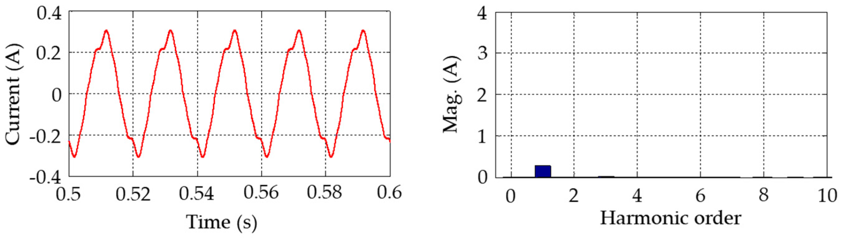
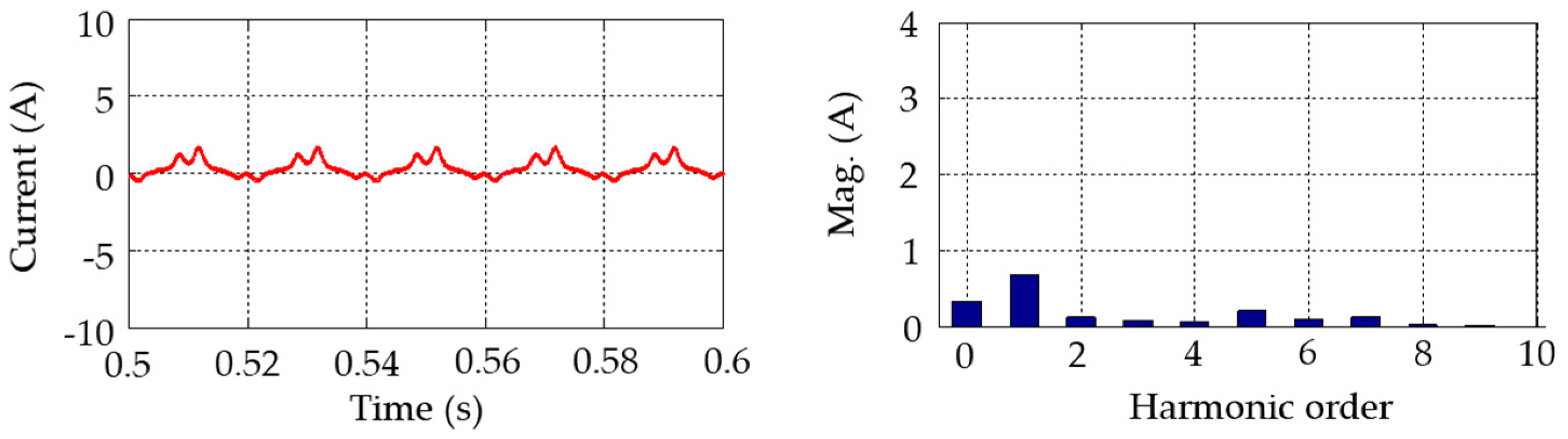
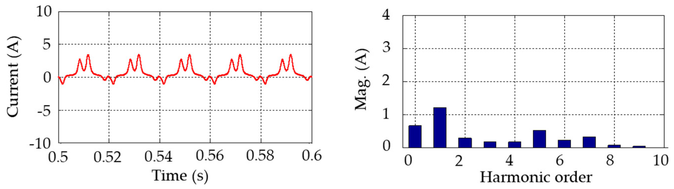
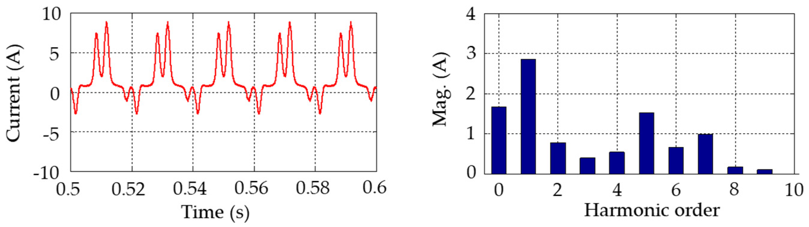
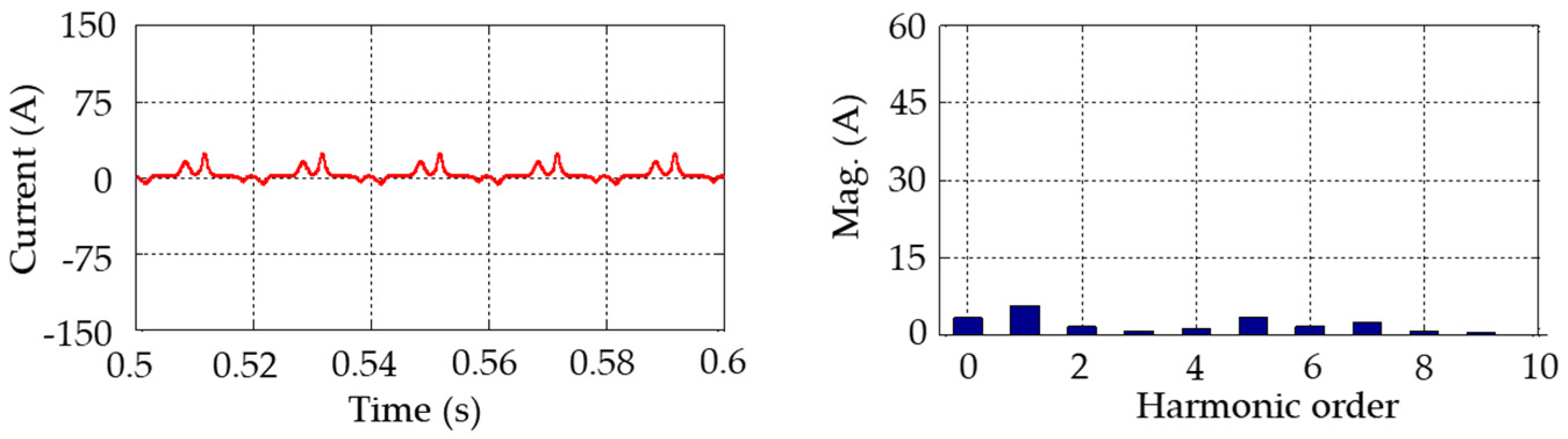
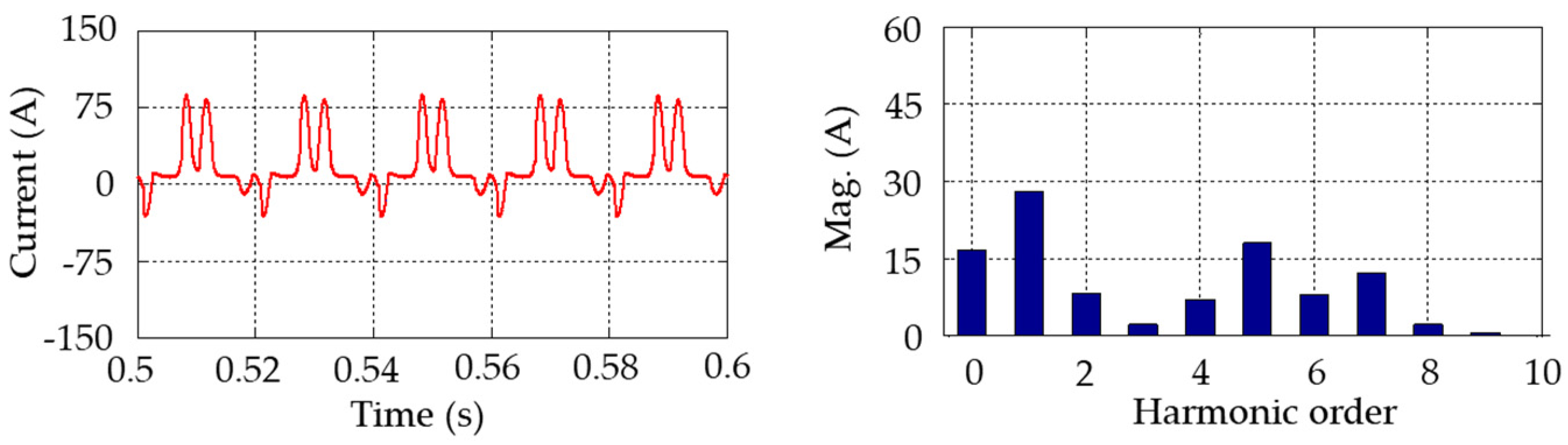
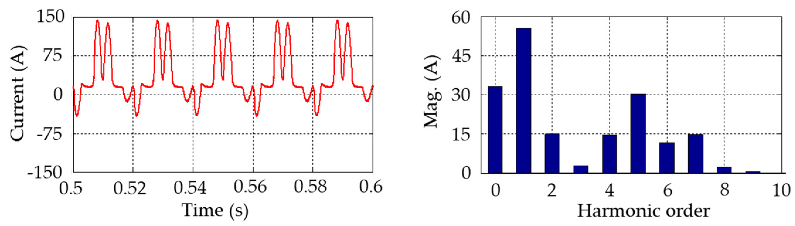
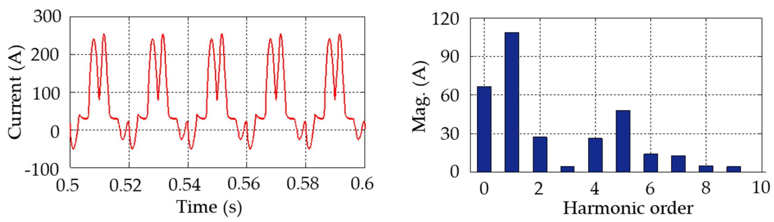
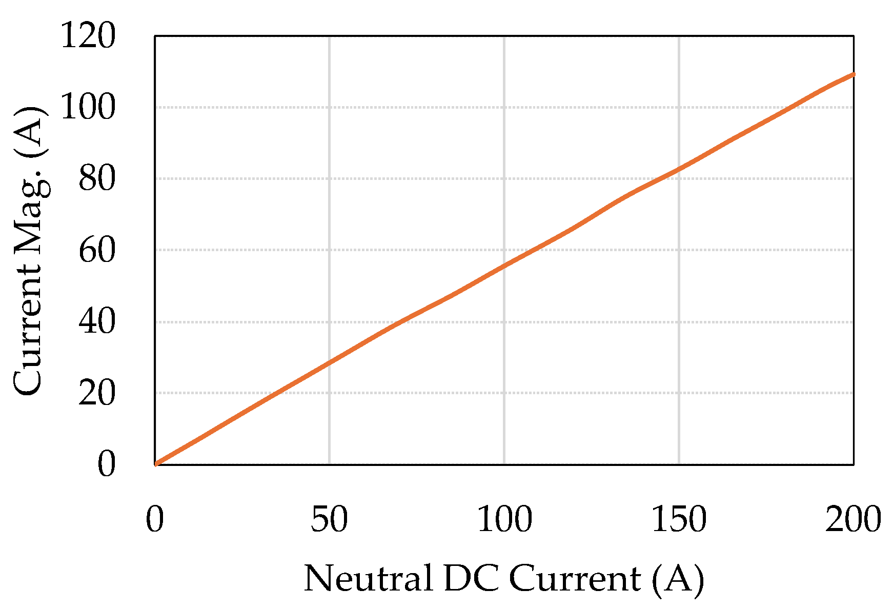
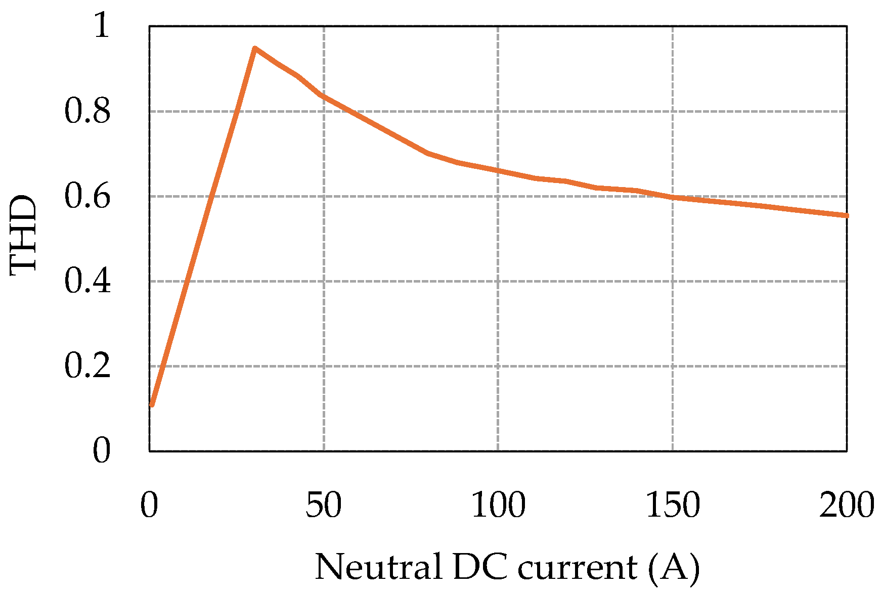
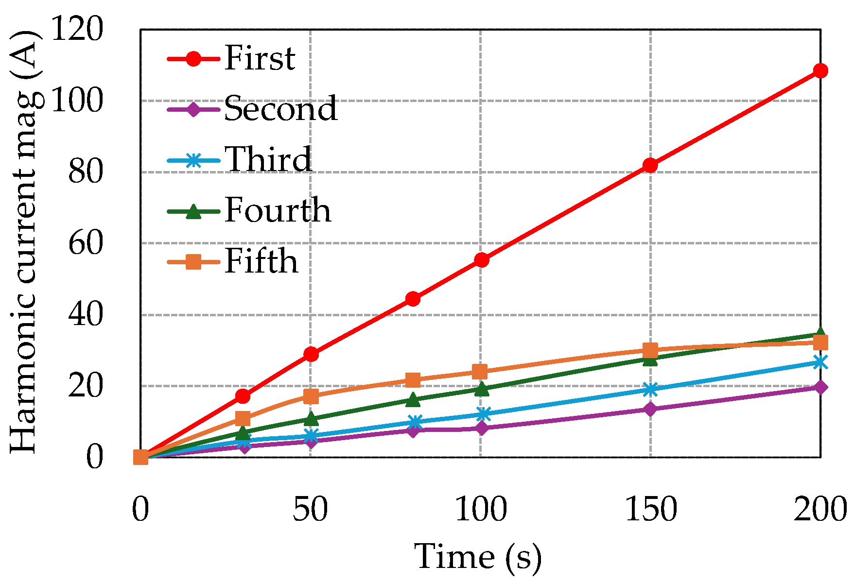
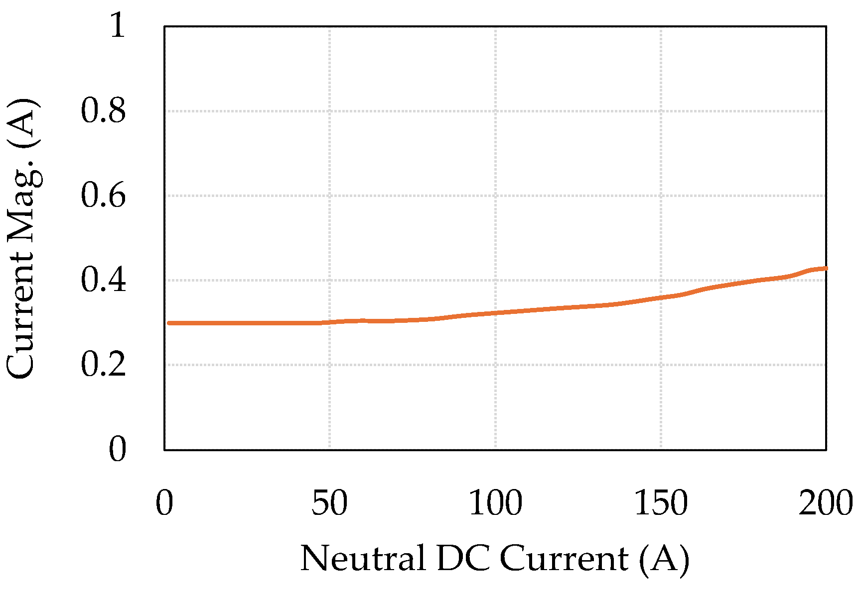
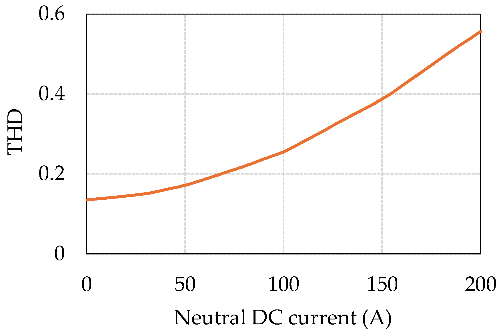
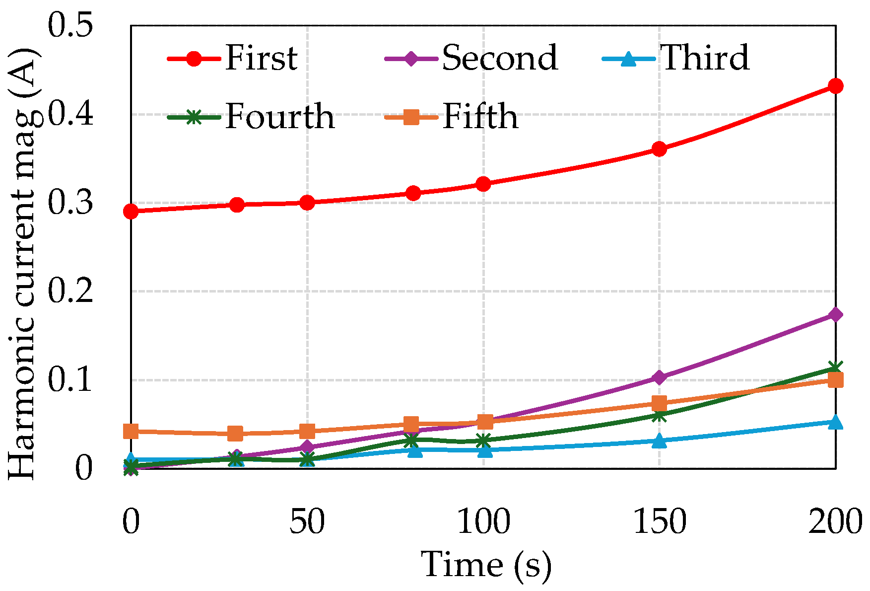
Regarding the GIC effects on specific transformer types, the following conclusions were reached. Under DC injection, the no-load current gets distorted. For a five-leg transformer with a neutral DC varying from 0 A to 200 A, the fundamental current exhibits a linear increase with the DC. The five-leg transformer shows a high degree of sensitivity to the GIC, even at low GIC magnitudes.