A Comparative Analysis of Price Forecasting Methods for Maximizing Battery Storage Profits

Abstract

Battery energy storage systems (BESS) rely on accurate electricity price forecasts to maximize arbitrage profits in day-ahead markets. We examined whether specific forecasting models, ranging from statistical benchmarks to machine learning methods, consistently deliver superior financial outcomes for storage operators. Using real market data from the Italian day-ahead electricity market over 2020–2024, we compared univariate singular spectrum analysis (SSA), ARIMA, SARIMA, random forests, and a 30-day simple moving average under a unified trading framework. All models were evaluated based on their ability to generate arbitrage profits. Univariate SSA clearly outperformed all alternatives, achieving on average 98% of the theoretical maximum profit while maintaining the lowest forecast error. Among the other models, simpler approaches performed surprisingly well: they achieved comparable, if not superior, profit performance to more complex, hour-specific, or computationally intensive configurations. These results were robust to plausible variations in battery parameters and retraining schedules, suggesting that univariate SSA offers a uniquely effective forecasting solution for battery arbitrage and that simplicity can often be more effective than complexity in operational revenue terms.

1. Introduction

Battery storage operators in day-ahead electricity markets rely heavily on price forecasting to guide their charge–discharge decisions. Accurate forecasts enable an arbitrage strategy of buying electricity when prices are low and selling when prices are high, directly influencing the profitability of storage assets. A broad array of forecasting methods—from classical time-series models like ARIMA to machine learning and hybrid approaches—have been applied to predict electricity prices, and the literature is rich with studies aiming to improve prediction accuracy. However, model performance in these studies is typically judged by statistical error metrics, with far less attention to the actual economic outcomes that better forecasts might yield.

Despite the extensive work on improving forecast accuracy, relatively few studies have explicitly linked forecasting quality to realized arbitrage profits for battery energy storage. It is often assumed that a more accurate forecast will automatically translate into higher trading gains, but the recent research [1] suggests this relationship is not straightforward. Indeed, many prior analyses stop at reporting standard error metrics without undertaking rigorous out-of-sample trading simulations to verify whether lower prediction errors actually translate into higher profits. Moreover, comparisons between simple and complex forecasting models under real market constraints are scarce. As a result, it remains unclear if sophisticated algorithms truly offer a profit advantage over basic benchmarks once realistic operational limitations and market conditions are taken into account.

To address these gaps, the present study examines whether specific price forecasting models consistently yield higher arbitrage revenues for battery storage operators and whether increased model complexity brings improved financial outcomes. We conduct a comprehensive backtesting experiment on the Italian day-ahead electricity market from 2020 to 2024, simulating a battery energy storage system that submits optimal bids under realistic operational constraints. Five forecasting approaches of varying complexity are compared—singular spectrum analysis (SSA), ARIMA, SARIMA, random forest, and a simple moving average—by using each model’s price forecasts in an optimization model that derives the battery’s optimal daily charge–discharge strategy. By tracking the realized profits from these forecast-driven strategies over several years, we assess which models consistently outperform the others in economic terms. This profit-oriented evaluation directly links forecasting model choice to financial performance, providing novel insight into whether advanced predictive techniques offer tangible value for energy storage arbitrage.

The rest of this paper is structured as follows. Section 2 reviews the literature. Section 3 presents the forecasting approaches and the optimization model adopted in the empirical analysis. Section 4 and Section 5 report, respectively, the simulation results and the robustness tests. Section 6 discusses and interprets the empirical findings, and Section 7 draws the conclusions.

2. Literature Review

Electricity price forecasting is essential for battery-storage operators, who rely on price expectations to make lucrative trading decisions. Good forecasts let them earn gains from arbitrage by buying and storing power when prices are low and selling when prices are high. This need is even greater in day-ahead markets, where operators must place their offers before the electricity is produced and used the next day. Because of this significance, the research on price forecasting models is both extensive and constantly developing; for useful summaries see also [2,3,4,5,6,7,8].

Price-forecasting techniques are commonly classified into two broad families: classical econometric models and artificial-intelligence (AI) or machine-learning approaches. Within the econometric family, time-series specifications such as autoregressive integrated moving average (ARIMA) and generalized autoregressive conditional heteroskedasticity (GARCH) remain popular because they capture linear dependence structures and conditional volatility using only historical observations.

Recent advances in econometric modeling for electricity price forecasting include the following. Parmezan et al. [9] and Makridakis et al. [10] show that ARIMA often requires less computational effort than many machine-learning alternatives and can, in certain contexts, deliver superior predictive accuracy, albeit at the cost of laborious hyper-parameter calibration. To enhance point forecasts, Zou and Yang [11] employ a dynamically weighted combination of several econometric models, while Ghasemi et al. [12] demonstrate that ARIMA is particularly effective for short-term price horizons. Complementarily, Ziel and Steinert [13] underscore the usefulness of GARCH processes for modeling price volatility. On the intraday front, Kiesel and Paraschiv [14] propose an econometric framework tailored to continuous trading, and Uniejewski et al. [15] adapt the least absolute shrinkage and selection operator (LASSO) of Tibshirani [16] to high-frequency electricity price data.

Although statistical models have proven effective in many forecasting tasks, they often struggle to capture nonlinear or highly complex dynamics. In response, AI-based models have gained prominence for their capacity to model nonlinearities, particularly under volatile conditions. These models are increasingly integrated with traditional approaches, forming hybrid methods that combine their respective strengths. By jointly modeling linear and nonlinear dependencies, hybrid models frequently yield improved predictive performance. A comprehensive survey of AI-based and hybrid methods is proposed by Nowotarski and Weron [6]. Some hybrids combine multiple AI techniques: for instance, Rafiei et al. [17] use clonal selection, wavelet transforms, and extreme learning machines for probabilistic forecasts, while Bara and Oprea [18] integrate random forest alongside gradient boosting methods in a weighted ensemble to improve day-ahead price forecasts under volatile conditions.

Early efforts to merge ARIMA with neural networks include those by Babu and Reddy [19] and Zhang [20], while Panigrahi and Behera [21] enhance exponential smoothing with artificial neural network for time-series forecasting. Chaabane [22] proposes a hybrid combining ARIMA with neural networks. Recent contributions by Alkawaz et al. [23] and Bissing et al. [24] apply hybrid methods to hourly day-ahead prices by integrating machine learning with multiple linear regression. In the New Zealand intraday market, Kapoor and Wichitaksorn [25] find that statistical models, especially those enhanced with LASSO, may outperform machine learning alternatives. Jiang et al. [26] extend this idea by embedding LASSO within neural networks and tree-based models.

A separate line of research considers singular spectrum analysis (SSA), a non-parametric method popularized by Golyandina et al. [27] that decomposes time series into trend, oscillatory, and noise components. SSA is often described as “model-free” because it does not assume a specific functional form but instead derives its structure from the data through eigen-decomposition of the trajectory matrix. Among the earliest applications to electricity markets, Miranian et al. [28] used SSA to predict day-ahead prices in the Spanish and Australian markets, achieving higher accuracy than traditional methods. More recently, SSA has been integrated with AI techniques, as a preprocessing step for improving forecasting performance: Zhang et al. [29] embed SSA within a support vector machine framework, while Zhu et al. [30] and Jiang and Sun [31] combine SSA with long short-term memory (LSTM) networks. Although their application to electricity price forecasting has been relatively limited, the existing evidence suggests that SSA-based methods, whether standalone or hybrid, represent a promising alternative. Our study extends this literature by evaluating the SSA technique not only on its forecasting accuracy but also on the realized arbitrage profits obtained when a battery-storage operator optimizes charge–discharge decisions using SSA-based price forecasts.

3. Methods

This section outlines the methodology used to evaluate the forecasting models under study. Statistical and econometric approaches, including simple moving average, ARIMA, and SARIMA, are described in Section 3.1; random forest models are detailed in Section 3.2; and the singular spectrum analysis procedure is presented in Section 3.3. The profit optimization model used to quantify arbitrage revenues is described in Section 3.4.

The input data comprise all hourly day-ahead electricity prices for the Sardinian bidding zone between 2014 and 2024 (for random forest estimation) and 2019 and 2024 (for statistical, econometric, and SSA models), obtained from the official records of the Italian power exchange maintained by Gestore del Mercato Elettrico (GME).

3.1. Statistical and Econometric Models

This group gathers three widely used forecasting families: simple moving average (SMA), non-seasonal autoregressive integrated moving average models (ARIMA), and their weekly seasonal extension (SARIMA).

3.1.1. Simple Moving Average

For every hour within the sample window, the one-step-ahead price forecast is obtained as the arithmetic mean of the corresponding hourly observations recorded over the previous 30 days (i.e, over the last month). Namely, for each clock hour $h\in \{1,\dots ,24\}$, the 30-day simple moving average forecast is

$${\widehat{p}}_{d,h}^{\mathrm{SMA}}={\displaystyle \frac{1}{30}}\sum _{j=1}^{30}{p}_{d-j,h},$$

where $p_{d-j,h}$ denote the electricity price recorded in hour h on day $d-j$. The resulting hourly predictions ${\widehat{p}}_{d,h}^{\mathrm{SMA}}$ are used to define the storage operator’s bidding strategy in the auction taking place on day $d-1$, which determines the dispatch schedule for electricity to be delivered on day d. The simple moving average contains no tuned hyper-parameters and serves as a parsimonious baseline.

3.1.2. ARIMA and SARIMA

Hourly price series ${\left\{p_{d,h}\right\}}_d$ were rendered stationary, where required, by applying regular differencing of order $d\in \{0,\dots ,7\}$. Candidate ARIMA$(p,d,q)$ and SARIMA$(p,d,q)(P,D,Q)\left[7\right]$ structures were screened by exhaustive search over $p,q,P,Q\in \{0,\dots ,7\},$ selecting the specification that minimized the corrected Akaike information criterion (AIC). The search follows the classical Box–Jenkins protocol, with upper bounds consistent with those employed by Papaioannou et al. [32]. Weekly seasonality ($s=7$) was imposed on SARIMA because Italian electricity prices exhibit a strong intra-week cycle.

3.1.3. Hourly Versus Modal Parameterization

Two layouts were compared.

Hourly variant: This “multi-set” strategy consists of calibrating and applying the best-performing parameter vector for each hour separately. For each year y and each hour h, a separate AIC-optimal model was estimated on the hour-h training window, thereby capturing the peculiar dynamics at that hour. Hourly forecasts were then generated by recursively iterating the fitted model. This method explicitly accommodates the heterogeneous price behavior observed across the 24 intra-day series.

Modal variant. This “one-set” approach applies a single parameter vector, defined as the modal (most frequently selected) order among the 24 h-specific models estimated in the preceding year. Concretely, the mode of the hourly orders, $(\overline{p},\overline{d},\overline{q})\mathrm{and}(\overline{P},\overline{D},\overline{Q}),$ in year $y-1$ was extracted and re-used as a common specification for all hours in year y. By relying on the parameters that appear most often across hours, the modal strategy provides a generalized forecast, in contrast to the hourly variant, which tailors a distinct optimal order to each individual series.

The ARIMA and SARIMA orders used for price forecasting are listed in Appendix A.

3.1.4. Rolling Training Window

In energy price forecasting, rolling windows enable continuous model updates that incorporate the latest data. They are particularly valuable when seasonality or cyclicality is present, allowing the model to follow current patterns rather than long-term averages. Rolling-window strategies have been employed in hybrid electricity price forecasting also by Ugurlu et al. [33], and De Marcos et al. [34], while Gunduz et al. [35] extend the approach with neural networks and transfer learning. The effect of training window length on forecast precision is explored by Fezzi and Mosetti [36] and Sbaraglia et al. [1]. Following evidence in Sbaraglia et al. [1,37] and Papaioannou et al. [32], a rolling window of $\Delta =365$ days was deemed sufficient. Let $\tau$ denote the delivery day to be predicted. Each re-estimation used only the prices from the preceding $\Delta$ days (that is, from $\tau -\Delta$ up to and including the day before $\tau$). By refitting the model daily on this rolling window, no information from day $\tau$ could leak into its own forecast. The same window length and update frequency were applied to ARIMA and SARIMA, ensuring a common information base.

3.2. Random Forest Models

Random forests (RF) were adopted as the non-parametric learning benchmark. The algorithm follows the original bootstrap-aggregation scheme of Breiman [38]. Two alternative specifications were investigated: an hourly design that fits twenty-four independent ensembles, one for each hour of the day, and a global design that calibrates a single ensemble on the stacked 24-h series. Both variants share the same data window, feature set, and re-training schedule, differing only in the treatment of the hour index.

3.2.1. Data and Pre-Processing

Let $p_{d,h}$ denote the realized price on day d and hour $h\in \{1,\dots ,24\}$. Two random forest specifications were estimated:

Global model: a single regressor fitted to the concatenated 24-h series;

Hourly model: twenty-four independent regressors, each fitted to the price series of a single hour.

Because the two layouts imply different temporal neighborhoods, the lagged predictor was defined accordingly:

• Global RF: one-step autoregressive term ${\ell }_{d,h}^{\mathrm{global}}=p_{d,h-1}$ with ${\ell }_{d,1}^{\mathrm{global}}=p_{d-1,24}$ by convention. The shift operates on the concatenated table, so it always points to the immediately preceding hour, even across day boundaries.
• Hourly RF: one-day lag at the same clock hour, ${\ell }_{d,h}^{\mathrm{hourly}}=p_{d-1,h}$. Each hour-specific file is ordered by calendar date only, so the time shift refers to the previous day.
• Calendar dummies (common to both variants): clock hour (h, global only), day of week (${\mathrm{dow}}_d$), and month (${\mathrm{mo}}_d$).
• Linear trend: ordinal position of day in its calendar year ($t_d$).

3.2.2. Hourly Ensembles

For each hour h, the training sample ${\mathcal{D}}_h^{\left(y\right)}=\{({\mathbf{x}}_{d,h},p_{d,h}):d\le 31\mathrm{December}y-1\}$ was used to estimate an ensemble ${\widehat{f}}_h^{\left(y\right)}(·)=\frac{1}{N_{\mathrm{tree}}}{\sum }_{j=1}^{N_{\mathrm{tree}}}{T}_{j,h}^{\left(y\right)}(·)$ with $N_{\mathrm{tree}}=500$, maximum feature fraction $\sqrt{\left|\mathbf{x}\right|}$, and minimum terminal node size equal to 2. The predictor vector ${\mathbf{x}}_{d,h}$ comprised $({\ell }_{d,h},{\mathrm{dow}}_d,{\mathrm{mo}}_d,t_d)$. The model was re-estimated five times ($y=2020,\dots ,2024$) following a rolling-origin protocol; each re-fit produced one-year-ahead forecasts ${\widehat{p}}_{d,h}={\widehat{f}}_h^{\left(y\right)}\left({\mathbf{x}}_{d,h}\right)$ for $d\in \mathrm{year}y$.

3.2.3. Global Ensemble

A single ensemble ${\widehat{f}}^{\left(y\right)}(·)=\frac{1}{N_{\mathrm{tree}}}{\sum }_{j=1}^{N_{\mathrm{tree}}}{T}_j^{\left(y\right)}(·)$ was instead trained on the pooled set ${\mathcal{D}}^{\left(y\right)}={\bigcup }_{h=1}^{24}{\mathcal{D}}_h^{\left(y\right)}$ using the expanded predictor ${\mathbf{z}}_{d,h}=(h,{\ell }_{d,h},{\mathrm{dow}}_d,{\mathrm{mo}}_d,t_d)$, where the hour index h acts as an additional categorical feature. All other hyper-parameters matched those of the hourly runs.

3.2.4. Training Regime

Both the hourly and the global RF models were re-estimated once per calendar year. For a given forecast year y, the learning sample comprised all observations up to and including 31 December $(y-1)$; no price information from year y was used in the estimation for that same year. Hence, for any target date $\tau \in [1\mathrm{January}y,31\mathrm{December}y]$ the conditioning set is

$$\left\{{\mathbf{x}}_{d,h}:d\le 31\mathrm{December}(y-1)\right\},$$

which ensures that every forecast respects the day-ahead decision timeline and is strictly out-of-sample with respect to the calendar year being predicted. Ensembles were fitted with the scikit-learn implementation and a fixed random seed to ensure replicability; the main hyper-parameters are summarized in

Table 1. Key settings adopted for the hourly and global random forest models.

Parameter	Value
Number of trees ($N_{\mathrm{tree}}$)	500
Maximum depth	Unlimited (nodes split until pure)
Maximum feature fraction	$\sqrt{\left|\mathbf{x}\right|}$
Minimum leaf size	2 observations
Retraining schedule	1 January 2020 → 2024 (five annual re-fits)

.

3.3. Singular Spectrum Analysis

Singular spectrum analysis (SSA) is a powerful tool within the realm of classical time-series analysis, combining techniques from multivariate statistics, geometry, dynamical systems, and signal processing. It provides a flexible and robust framework for decomposing time series into interpretable components, such as smooth trends, periodic patterns, and stochastic noise. SSA has demonstrated remarkable effectiveness and versatility, as evidenced by over a hundred studies spanning various fields and applications. For a comprehensive overview of SSA methodology, refer to [27,39].

3.3.1. SSA Decomposition

Let ${\mathbf{y}}_N=\{y_1,\dots ,y_N\}$ denote a univariate time series of length N. SSA decomposition begins by transforming the time series into a structured matrix form, followed by matrix decomposition and reconstruction steps that isolate distinct components such as trend, oscillations, and noise. The overall process is outlined below.

1.

Embedding: Choose a window length parameter L such that $2\le L\le N-1$, and define $K=N-L+1$. Construct the trajectory (Hankel) matrix $\mathbf{Y}\in {\mathbb{R}}^{L\times K}$, where each column is a lagged segment of the original series:

$$\mathbf{Y}=\left[\begin{array}{cccc}{y}_1& y_2& \dots & y_K\\ y_2& y_3& \dots & y_{K+1}\\ ⋮& ⋮& \ddots & ⋮\\ y_L& y_{L+1}& \dots & y_N\end{array}\right]$$

2.

Singular Value Decomposition (SVD): Decompose the matrix $\mathbf{Y}$ using SVD into a sum of rank-one matrices: $\mathbf{Y}={\mathbf{Y}}_1+\dots +{\mathbf{Y}}_d$.

3.

Grouping: Partition the set of elementary matrices into m disjoint groups $I_1,\dots ,I_m$, and form grouped matrices by summing the elements within each group. In the simplest case ($m=2$), group $I_1=1,\dots ,r$ is associated with the signal (e.g., trend and periodicity), and $I_2=r+1,\dots ,d$ corresponds to noise.

4.

Diagonal Averaging (Reconstruction): Transform each grouped matrix ${\mathbf{Y}}_{I_j}$ back into a time series of length N via diagonal averaging (also known as Hankelization). This step reconstructs the components of the original series.

The reconstructed vectors $\left\{{\tilde{y}}_{j_1},\dots ,{\tilde{y}}_{j_N}\right\}$ represent the denoised or decomposed components of the original time series and can be used for further analysis. One primary objective of time series analysis is forecasting. The next section addresses forecasting using SSA.

3.3.2. Forecasting by SSA

The fundamental requirement for applying SSA forecasting is that the time series satisfies a Linear Recurrent Formula (LRF). A time series $Y_N=(y_1,\dots ,y_N)$ satisfies an LRF of order d if

$$y_t=a_1{y}_{t-1}+a_2{y}_{t-2}+\dots +a_d{y}_{t-d},\mathrm{for}t=d+1,\dots ,N.$$

(1)

Although several variations of SSA forecasting algorithms exist, we focus here on one of the most widely used approaches: the Recurrent Method.

Let ${\sigma }_1\ge \dots \ge {\sigma }_r$ be the r largest singular values of the trajectory matrix, and let $U_1,\dots ,U_r$ be the corresponding eigenvectors. Let $U_j^{▿}$ denote the vector consisting of the first $L-1$ components of the eigenvector $U_j$, and let ${\pi }_j$ be its last component, for $j=1,\dots ,r$. Define ${\upsilon }^2={\sum }_{j=1}^r{\pi }_j^2$, and use this to construct the coefficient vector $\mathfrak{R}$ as

$$\mathfrak{R}={\displaystyle \frac{1}{1-{\upsilon }^2}}\sum _{j=1}^r{\pi }_j{U}_j^{▿}=\left(\begin{array}{c}{a}_1\\ ⋮\\ a_{L-1}\end{array}\right).$$

(2)

Using this notation, the one-step-ahead univariate SSA forecast ${\widehat{y}}_{N+1}$ is given by

$${\widehat{y}}_{N+1}=a_1{\tilde{y}}_N+a_2{\tilde{y}}_{N-1}+\dots +a_{L-1}{\tilde{y}}_{N-L+2},$$

(3)

where ${\tilde{y}}_{N-L+2},\dots ,{\tilde{y}}_N$ are the reconstructed values from the SSA decomposition (as obtained in Step 4: Diagonal Averaging).

3.3.3. SSA Choices

As observed in the SSA method for this study, two parameters, L and r, need to be specified. Although there are several studies addressing the methodology for choosing these parameters, there is no proof regarding which values are optimal. In this study, we have considered a grid search for both parameters and identified the best values corresponding to the minimum error for one-step ahead forecasts. We searched within the range $24\le L\le 65$ and $3\le r\le 14$ to find the optimal values of these parameters:

$$\mathrm{optimal}(L,r)=\underset{L\in \{24,\dots ,65\},r\in \{3,\dots ,14\}}{argmin}\mathrm{Error}(L,r)$$

(4)

where $\mathrm{Error}(L,r)$ is the error for forecasting using a set of values $(L,r)$ from the expanded grid.

3.4. Profit Optimization Model

The proposed optimization model is designed for the optimal utilization of energy storage, given varying energy prices and storage capacities. The model is formulated to maximize profit from buying and selling energy by making optimal decisions on when to buy, sell, or store energy.

We first introduced this optimization approach in [37]. As in that framework, we assume a perfectly liquid energy market, meaning that a storage operator can purchase or sell any quantity of energy (up to an hourly limit) without altering the market price. The operator is thus considered a price taker; that is, its actions do not influence the market price.

In practice, the model proceeds on a rolling day-by-day basis, allowing the operator to submit offers for each of the 24 h in the following day. This day-by-day approach can entail negligible profit loss compared to an all-encompassing horizon, as suggested by Sbaraglia et al. [1,37], Connolly et al. [40]. A more substantial loss arises from price forecast inaccuracies, which can cause profit reductions relative to the ideal scenario with perfect price information.

The model works in discrete time. The time periods $(d,h)$ are expressed in days d and hours h. To ensure consistency across our dataset, all calendar days were normalized to a fixed 24-h structure, thereby eliminating distortions arising from daylight-saving transitions.

The model has the following input parameters: $p_{d,h}$ denotes the electricity price observed on day d during hour h; Q represents the storage unit’s energy capacity limit; k signifies the hourly power constraint, namely, the maximum volume of energy that can be bought or sold within a single hour; C denotes the unit holding cost accrued per hour of stored energy; $\alpha$ represents the hourly energy-retention loss (fade) expressed as a percentage of the stored quantity; $\beta$ signifies the fixed operating and maintenance expense incurred each hour to keep the storage facility functional; $\lambda$ denotes the transaction fee, specified as a constant proportion of the energy volume bought or sold.

The model uses the following three sets of decision variables. The variable $b_{d,h}$ represents the amount of energy purchased at time $(d,h)$. It can take any real value from 0 to k, that is, the maximum amount of energy that can be transferred (i.e., purchased or sold) in a single hour. The variable $s_{d,h}$ represents the amount of energy sold at time $(d,h)$, which can take any real value from 0 to k. Finally, the variable $e_{d,h}$ represents the amount of energy stored at the end of hour h of day d. It can take any real value from 0 to Q, where Q is the maximum storage capacity.

We consider the following constraints. The domain of definition of the decision variables is $b_{d,h}=s_{d,h}\in [0,k]$ and $e_{d,h}\in [0,Q]$. To ensure that the energy balance is consistent over time, it holds $e_{d,h}=e_{d,h-1}·(1-\alpha )+b_{d,h}-s_{d,h}$ for $h\in [2,24]$; and $e_{d,h}=e_{d-1,24}·(1-\alpha )+b_{d,h}-s_{d,h}$ for $h=1$. Furthermore, the energy sold at any hour cannot exceed the amount of energy stored in the previous hour, that is: $s_{d,h}\le e_{d,h-1}$ for $h\in [2,24]$; and $s_{d,h}\le e_{d-1,24}$ for $h=1$. Finally, the energy can either be purchased or sold at any given time, but not both simultaneously, so that if $b_{d,h}\ne 0\Rightarrow s_{d,h}=0$, and if $s_{d,h}\ne 0\Rightarrow b_{d,h}=0$.

The optimization problem is formulated to maximize aggregate revenues generated by the trading strategy, that is,

$$max\sum _d\sum _h[s_{d,h}·p_{d,h}·(1-\lambda )-b_{d,h}·p_{d,h}·(1+\lambda )-C·e_{d,h}-\beta ·Q]$$

(5)

where each term in the summation consists of the revenue earned at hour h of day d. Solving this optimization problem entails identifying the decision rule that maximizes the objective function over the feasible set, defined by all allocation strategies that satisfy the specified constraints.

4. Results

This section summarizes the main findings of our forecasting experiments, which cover hourly electricity prices for five calendar years (2020–2024). Each method is assessed by its revenue-generation capacity, defined as the profit a battery storage operator can earn when the forecast is paired with the profit optimization model for arbitrage trading described in Section 3.4. We also report two statistical measures: the root mean squared error (RMSE) and the multistep indicator proposed by Sbaraglia et al. [1], the latter assessing both goodness-of-fit and relevance for arbitrage profitability.

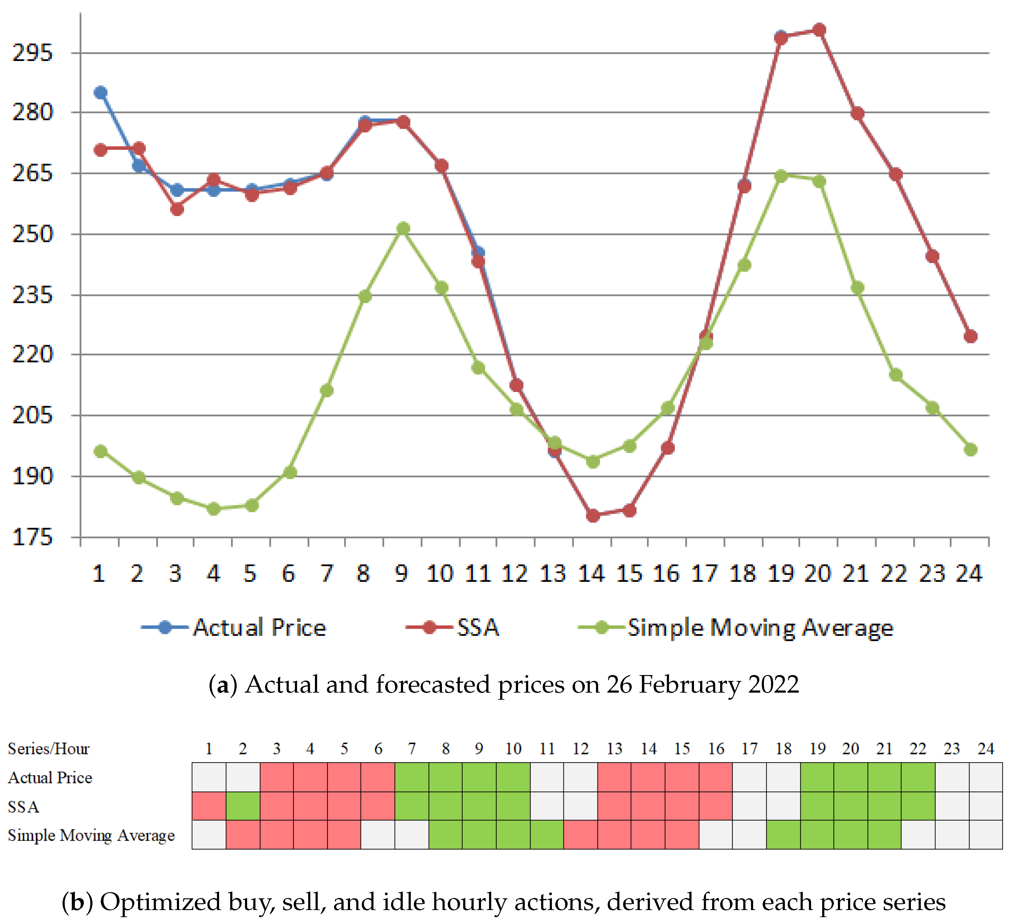
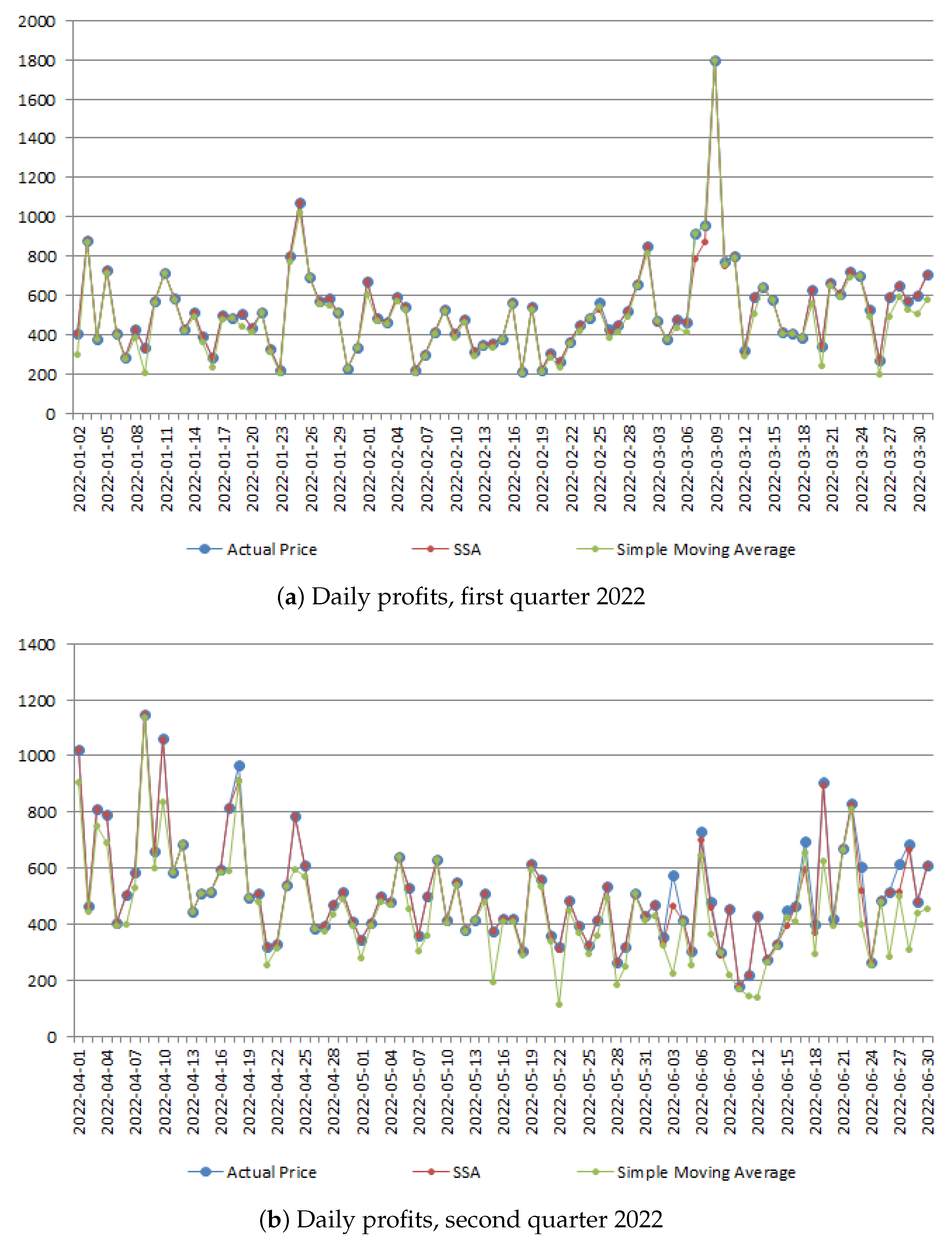
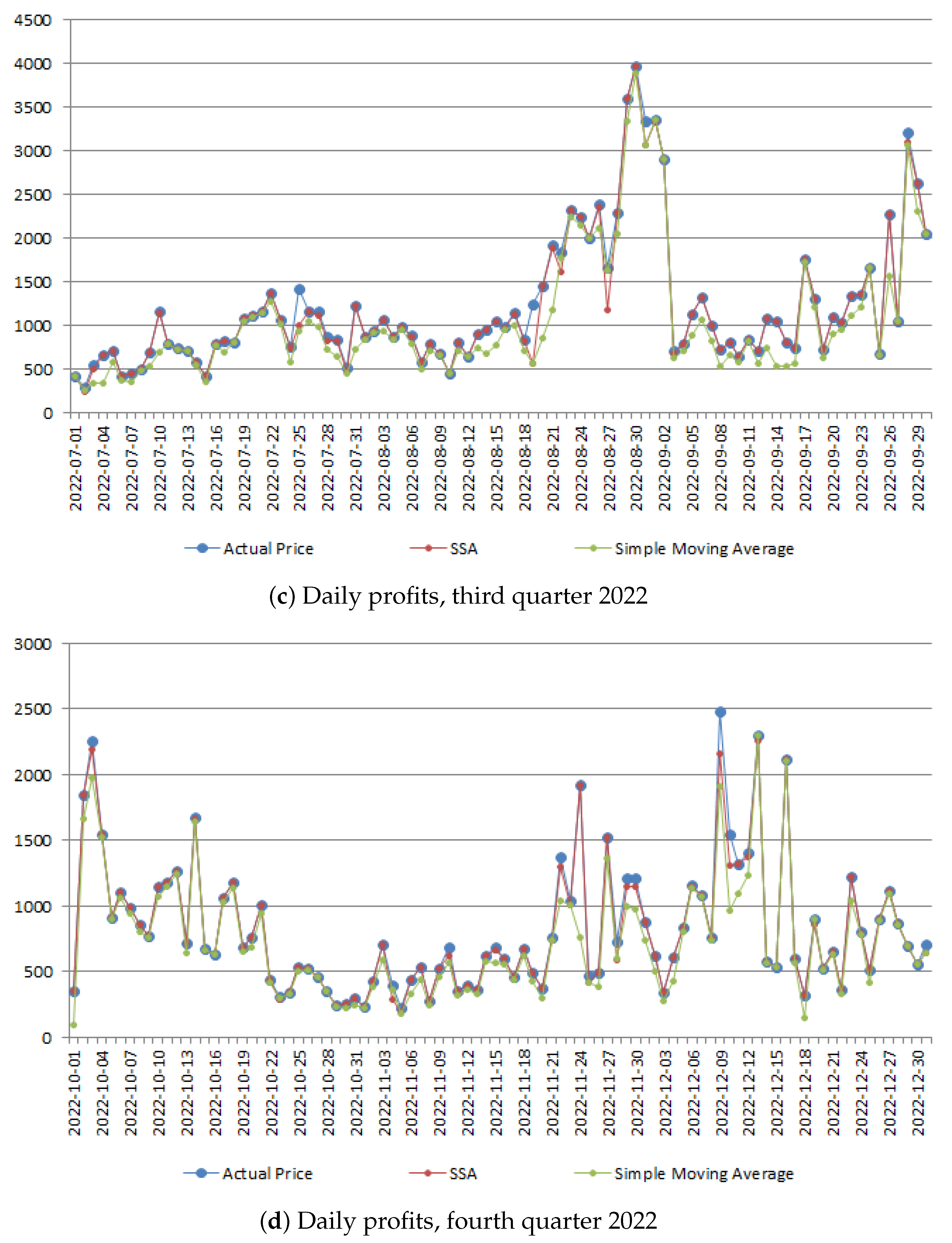
For every forecasting technique described in Section 3, we generated hourly price paths for the Sardinian price zone of the Italian day-ahead market over 2020–2024 and, with the profit-optimization model of Section 3.4, we determined the corresponding daily optimal arbitrage revenues. An illustrative example of how these profits are generated is provided in Appendix B.

The simulations assume a battery energy storage system (BESS) of 4 MWh total capacity, with a charge–discharge power limit of 1 MWh per hour. Hourly operating costs are set at €0.03 MWh; storage losses, transaction fees, and capital charges are ignored. These parameters mirror those adopted by Sbaraglia et al. [1,37], Agathokleous et al. [41] and accord with the minimum-capacity estimates by Münderlein et al. [42] for covering operating expenses.

Table 2. Profits obtained by optimizing trading strategies using each forecasting method (nominal euros).

Method	2020	2021	2022	2023	2024	Total
Theoretical Maximum	45,697	101,670	280,336	140,589	134,662	702,955
Simple Moving Average	39,341	91,540	250,490	129,125	125,963	636,460
ARIMA (hourly)	39,095	88,542	239,737	121,035	125,554	613,963
ARIMA (modal)	39,353	90,593	245,314	129,737	125,598	630,595
SARIMA (hourly)	38,811	89,839	243,886	121,353	124,225	618,114
SARIMA (modal)	39,751	91,858	241,167	129,737	125,383	627,896
Random Forest (hourly)	37,049	74,596	209,400	94,284	109,690	525,019
Random Forest (global)	38,377	88,777	242,695	122,723	118,227	610,799
Univariate SSA	44,287	98,714	275,059	138,282	132,565	688,906

Theoretical Maximum: profit achievable if trading decisions were optimised having perfect price foresight.

reports the annual profits obtained by optimizing trading strategies using each forecasting approach.

Table 3. Percentage of the theoretical maximum profit achieved when optimizing trading strategies using the price forecasts from each method.

	2020	2021	2022	2023	2024	2020–2024
Simple Moving Average	86.09%	90.04%	89.35%	91.85%	93.54%	90.54%
ARIMA (hourly)	85.55%	87.09%	85.52%	86.09%	93.24%	87.34%
ARIMA (modal)	86.12%	89.10%	87.51%	92.28%	93.27%	89.71%
SARIMA (hourly)	84.93%	88.36%	87.00%	86.32%	92.25%	87.93%
SARIMA (modal)	86.99%	90.35%	86.03%	92.28%	93.11%	89.32%
Random Forest (hourly)	81.07%	73.37%	74.69%	67.06%	81.45%	74.69%
Random Forest (global)	83.98%	87.31%	86.57%	87.29%	87.79%	86.89%
Univariate SSA	96.91%	97.09%	98.11%	98.35%	98.44%	98.00%

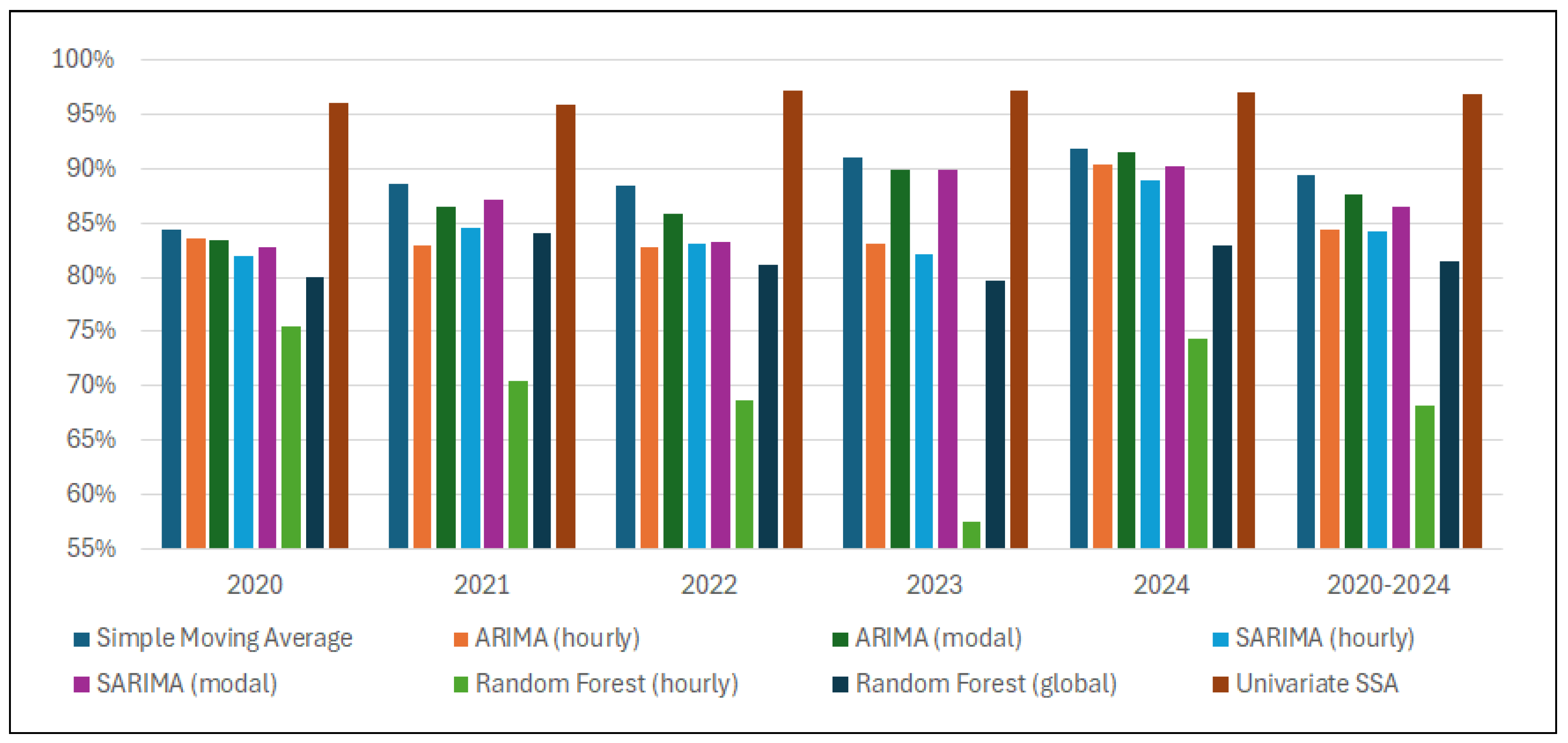
Background colors: red below 80%; light red between 80 and 85%; yellow between 85 and 90%; light green between 90 and 95%; and green above 95%.

presents each method’s profit as a share of the theoretical maximum attainable under perfect price foresight. Namely, we define theoretical maximum profit as the upper bound on revenue attainable when charge–discharge decisions are optimized with perfect knowledge of future day-ahead prices. This ideal benchmark allows us to assess how closely each forecasting method approaches perfect foresight. Figure 1 presents these results in visual form.

Across the five-year horizon, univariate singular spectrum analysis (SSA) stands out by a wide margin. Its realized profits consistently exceed 97% of the theoretical maximum in every individual year and average 98% over 2020–2024, indicating that the SSA decomposition captures the dominant price dynamics with minimal loss of arbitrage value.

Among the conventional benchmarks, the 30-point simple moving average performs surprisingly well: although it lags behind SSA in all years by a large margin, it still yields more than 90% of the perfect-foresight benchmark in three of the five years and averages 90.5% over the full sample. This outcome already hints at a broader pattern: models that favor parsimony and a single, general set of parameters often trade almost as profitably as (and sometimes better than) more intricate, hour-specific alternatives.

The econometric families offer a clear illustration. ARIMA and SARIMA in their “modal” variants (one global model whose optimal parameters are reused for every hour) reach average profit shares close to 89–90%. Their corresponding “hourly” variants, which re-estimate separate parameter sets for each of the 24 series, are slightly less effective in every year. Pooling information across hours therefore appears to stabilize inference and improve trading outcomes, even though the underlying specification remains linear.

Random forest methods sharpen this contrast. The global random forest model, trained a single time on the concatenated 24-h series, attains an average of 86.9% of the theoretical maximum—comparable to the econometric baselines—whereas the hourly random forest ensemble falls to 74.7%, with a particularly poor showing in 2023 (67%). Here, the penalty for a “multi-set” approach is severe: fitting 24 independent forests fragments the available data, fosters over-fitting, and erodes arbitrage value despite the lower RMSE observed for each separate hour (see

Table 4. Root mean square error delivered by each forecasting method, by calendar year.

Method	2020	2021	2022	2023	2024
Simple Moving Average	11.42	33.29	97.60	33.87	24.58
ARIMA (hourly)	10.56	25.40	75.52	28.11	22.29
ARIMA (modal)	10.58	25.51	75.19	27.34	22.35
SARIMA (hourly)	10.18	24.65	74.01	27.51	22.25
SARIMA (modal)	10.06	24.24	73.86	27.34	22.44
Random Forest (hourly)	12.64	90.14	178.79	39.18	26.42
Random Forest (global)	21.58	108.99	260.74	70.11	52.41
Univariate SSA	6.66	9.78	32.56	12.33	9.56

).

Taken together, the results reveal a consistent ordering. Univariate SSA yields the highest returns. A second, roughly equivalent tier is formed by the simple moving average benchmark, the “modal” ARIMA/SARIMA models, and the global random forest. Finally, well below these, the hourly random forest specification performs worst. The pattern underscores two points. First, the gap between SSA and the best non-SSA alternative widens during periods of heightened price volatility, implying that SSA’s data-adaptive decomposition is especially valuable when the market departs from regular daily patterns. Second, once a baseline level of accuracy is achieved, incremental complexity does not guarantee higher profit: broad, general models with a single parameter set can match or surpass hour-by-hour calibrations. This is confirmed by the analysis of root mean square error (RMSE).

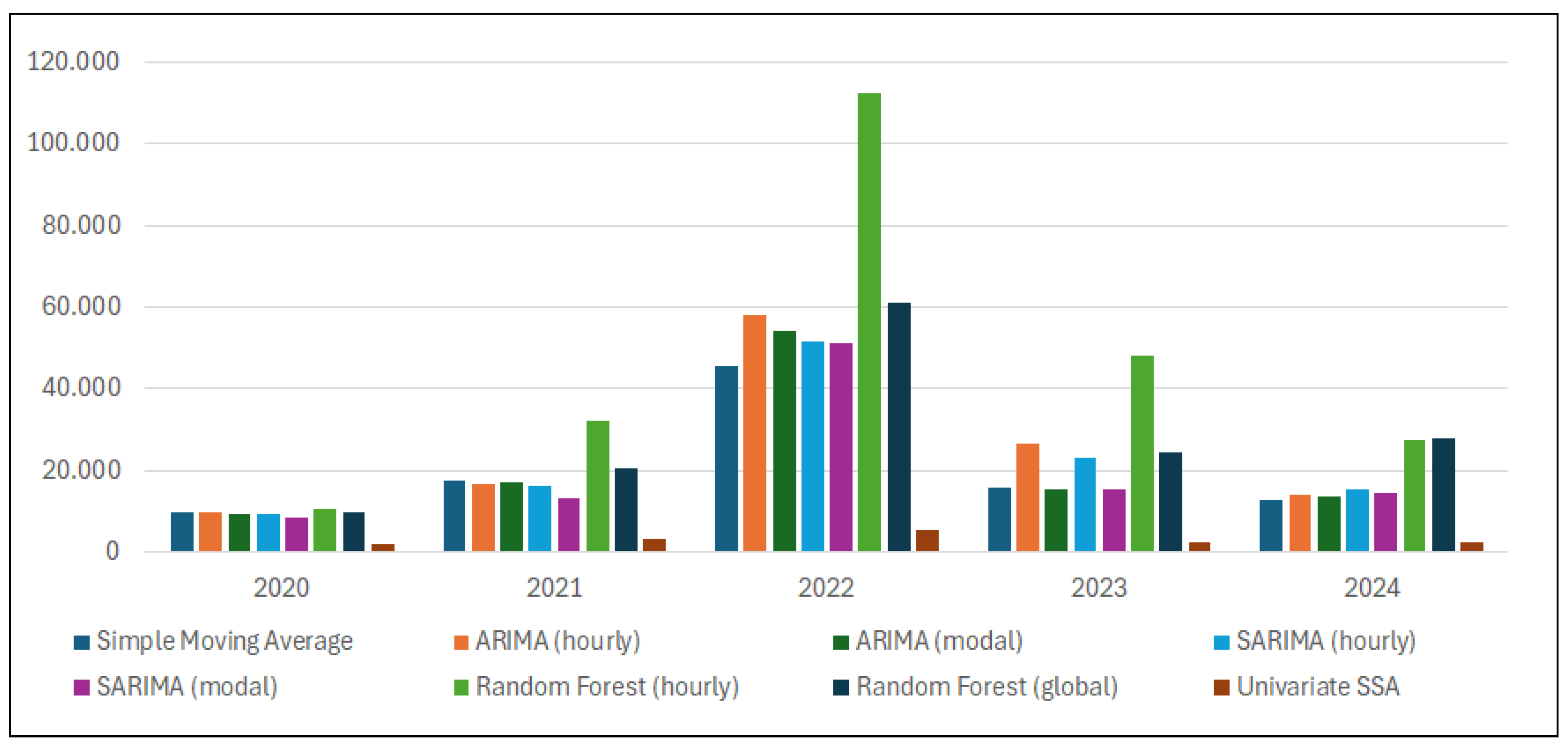
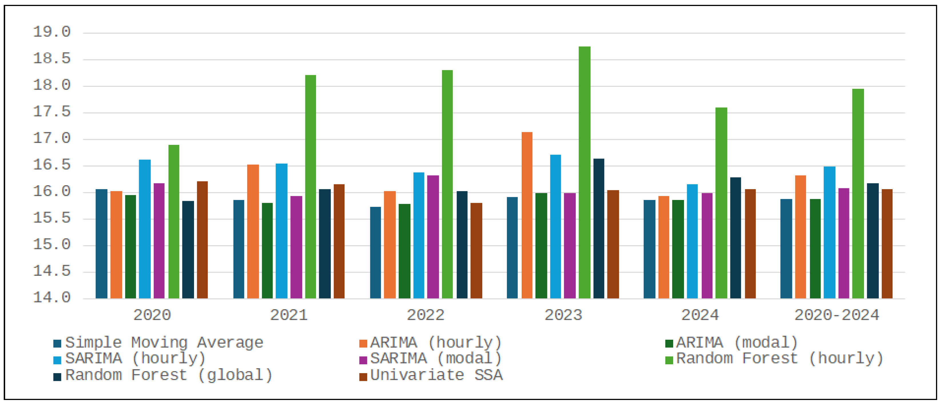
Table 4 reports the RMSE achieved by each forecasting method, with corresponding values also illustrated in Figure 2. Univariate SSA again stands out, but the remaining results confirm that statistical fit and trading value are only weakly related. ARIMA and SARIMA achieve markedly lower RMSEs than the simple moving average benchmark, yet their revenue shares of the theoretical maximum are similar and occasionally smaller. The contrast is sharper for the random forest pair: the hourly specification cuts RMSE by more than 40% relative to the global model but nonetheless generates consistently lower profit.

The mismatch arises because RMSE rewards point-wise level accuracy, whereas arbitrage rewards correct ranking and is spread over sequences of hours. The 24 independent hourly forests excel at reproducing each hour’s average price, but their hour-to-hour errors are uncorrelated; small misalignments can reverse the predicted price order and misguide the charge–discharge schedule. The single global forest, trained on the stacked 24-h series, allows cross-hour interactions; although its point forecasts are less precise in absolute terms, the errors are coherent and preserve the shape and timing of daily peaks and troughs, enabling more profitable trading decisions. A similar, though milder, pattern explains why the simple moving average matches or surpasses ARIMA/SARIMA profits despite inferior RMSE.

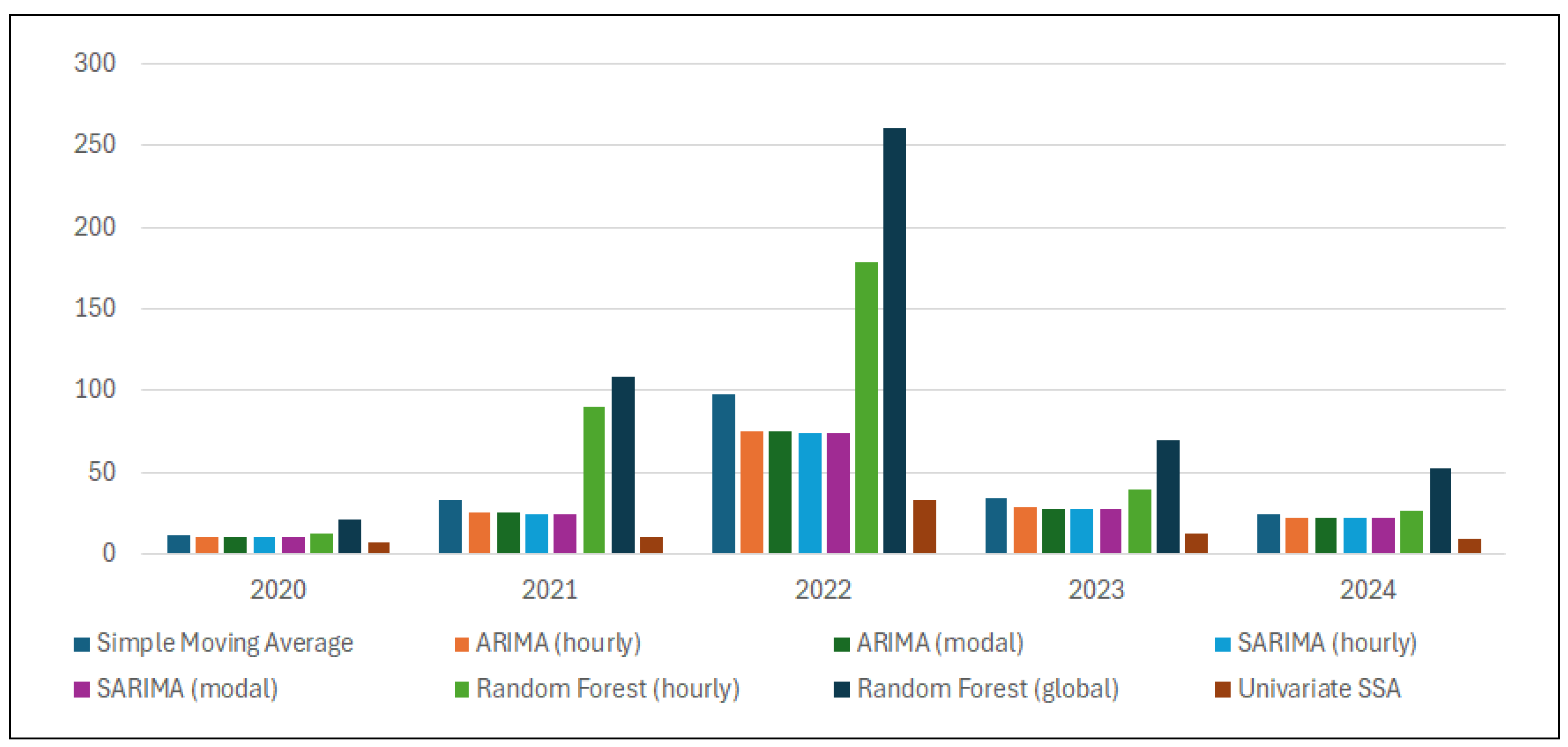
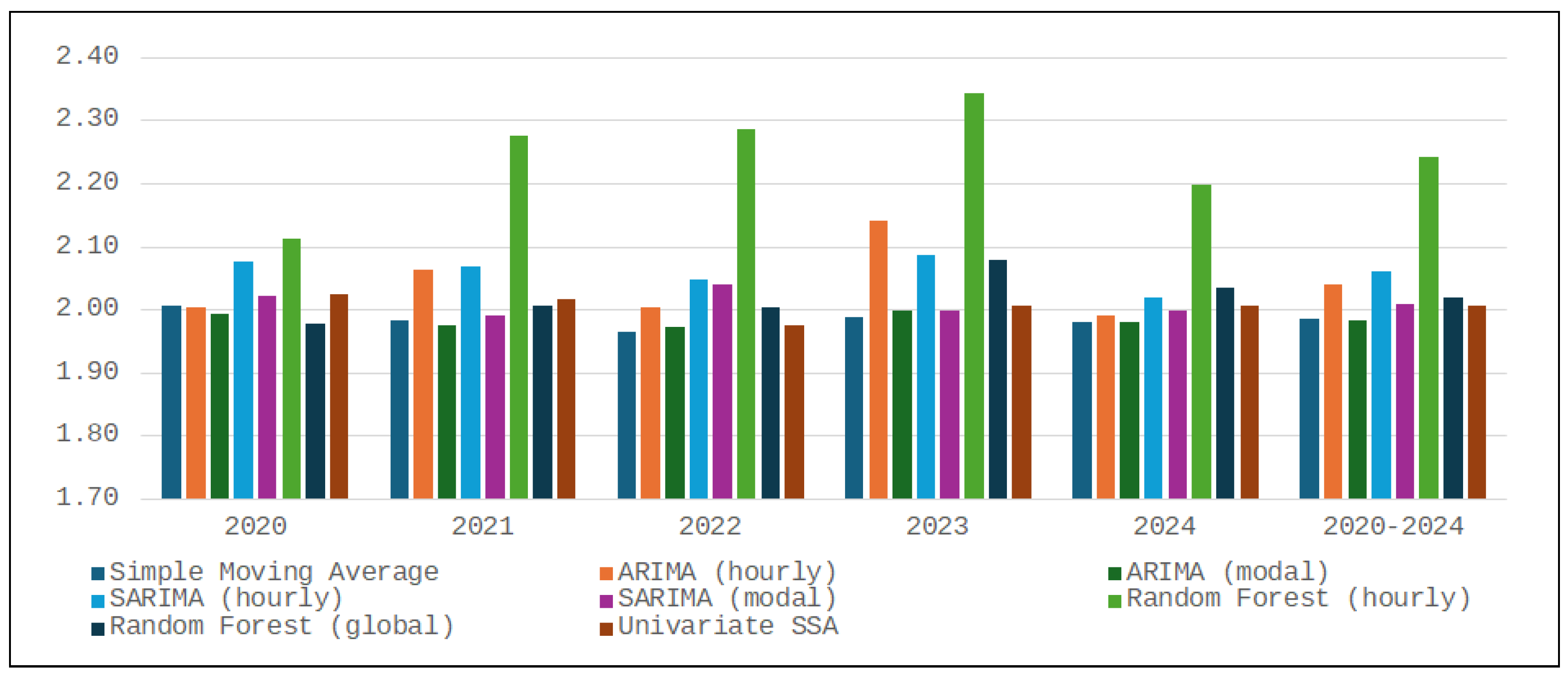
A metric that explicitly balances level error and trading relevance is the multistep indicator, which quantifies profit loss caused by imperfect price forecasts. Its values are reported in

Table 5. Values of the multistep indicator (lower is better) for each forecasting method, by calendar year.

Method	2020	2021	2022	2023	2024
Simple Moving Average	9779	17,516	45,380	15,605	12,532
ARIMA (hourly)	9580	16,763	57,932	26,655	14,079
ARIMA (modal)	9275	17,178	54,388	15,509	13,642
SARIMA (hourly)	9319	16,022	51,565	22,919	15,443
SARIMA (modal)	8360	13,205	50,947	15,509	14,332
Random Forest (hourly)	10,629	32,336	112,484	47,996	27,402
Random Forest (global)	9864	20,333	61,068	24,320	28,016
Univariate SSA	1768	3424	5516	2400	2249

, where lower scores generally indicate more profitable forecasting methods. Accordingly, the histogram in Figure 3 tends to mirror the trends in the profit distribution shown in Figure 1, with lower bars in one corresponding to higher bars in the other. This inverse relationship highlights the metric’s usefulness in identifying methods that yield greater profits for storage operators.

The multistep scores reproduce the same hierarchy observed for revenues: SSA remains an order of magnitude better than all alternatives, while the global random forest generally outperforms its hourly counterpart despite the latter’s lower RMSE. Thus, once baseline accuracy is achieved, further RMSE reductions do not necessarily improve arbitrage gains, whereas metrics that reward profitable temporal ordering, such as the multistep indicator, tend to reflect the profit-based ranking.

5. Robustness Tests

This section examines whether the profit hierarchy reported in Section 4 persists under plausible modifications of the experimental setting. First, in Section 5.1, we assess whether the dominance of univariate SSA, as well as the relative ordering of the remaining forecasters, survives when the battery’s charge–discharge power is doubled while energy capacity is held constant. Second, in Section 5.2, we test whether random forest performance improves when the retraining frequency is increased from annual to daily updates. Third, in Section 5.3, we analyze the sensitivity of our results to realistic battery-efficiency degradation, operation and maintenance charges, and transaction fees.

5.1. Doubling of Charge–Discharge Power

The key parameter for an energy-arbitrage battery operator is the power-to-energy ratio, that is, how quickly the system can deliver energy relative to the amount it can store.

Increasing this ratio by raising the charge–discharge power, while holding energy capacity constant, allows the battery to cycle faster and capture price spreads more effectively. By contrast, if both energy capacity and power are scaled by the same factor (leaving the ratio unchanged), the absolute arbitrage revenue for every forecasting method rises proportionally, but each method’s share of the theoretical maximum profit is unaffected.

Accordingly, we test robustness by doubling power while keeping capacity unchanged. In the baseline configuration, a 4 MWh battery charges or discharges at 1 MWh/h (with a ratio of 0.25/h), taking four hours to move from empty to full (or vice versa). In the robustness scenario, the power rating is increased to 2 MWh/h (with a ratio of 0.50/h), halving the cycle time to two hours and enabling the operator to exploit price spreads more aggressively.

Table 6. Profits obtained by optimizing trading strategies using each forecasting method (nominal euros). Charge–discharge power: 2 MWh/h.

Method	2020	2021	2022	2023	2024	Total
Theoretical Maximum	57,270	125,670	345,280	177,975	167,409	873,605
Simple Moving Average	48,373	111,305	305,258	161,905	153,689	780,529
ARIMA (hourly)	47,840	104,275	285,528	147,999	151,290	736,932
ARIMA (modal)	47,800	108,676	296,602	159,862	153,109	766,049
SARIMA (hourly)	46,892	106,234	287,099	146,241	148,792	735,258
SARIMA (modal)	47,399	109,488	287,521	159,862	151,047	755,317
Random Forest (hourly)	43,261	88,504	237,426	102,233	124,569	595,993
Random Forest (global)	45,824	105,680	280,257	141,897	138,799	712,458
Univariate SSA	54,986	120,438	335,796	172,974	162,493	846,688

Theoretical Maximum: profit achievable if trading decisions were optimised having perfect price foresight.

reports the theoretical maximum and the realized profits for each forecasting method under the 2 MWh/h setting. As expected, every model earns more in absolute terms than in the 1 MWh/h baseline (Table 2). Yet, as 

Table 7. Percentage of the theoretical maximum profit achieved when optimizing trading strategies using the price forecasts from each method. Charge–discharge power: 2 MWh/h.

	2020	2021	2022	2023	2024	2020–2024
Simple Moving Average	84.46%	88.56%	88.40%	90.97%	91.80%	89.35%
ARIMA (hourly)	83.53%	82.98%	82.69%	83.16%	90.37%	84.36%
ARIMA (modal)	83.46%	86.48%	85.90%	89.82%	91.45%	87.69%
SARIMA (hourly)	81.88%	84.53%	83.15%	82.17%	88.87%	84.16%
SARIMA (modal)	82.76%	87.12%	83.27%	89.82%	90.22%	86.46%
Random Forest (hourly)	75.53%	70.42%	68.76%	57.44%	74.40%	68.22%
Random Forest (global)	80.01%	84.09%	81.16%	79.72%	82.90%	81.55%
Univariate SSA	96.01%	95.83%	97.25%	97.19%	97.06%	96.92%

Background colors: red below 80%; light red between 80 and 85%; yellow between 85 and 90%; light green between 90 and 95%; and green above 95%.

and Figure 4 make clear, their relative rankings remain essentially unchanged, and as discussed below, the increased power widens rather than narrows the divide between parsimonious one-set models and their hour-specific counterparts.

The alternative battery configuration—doubling power to 2 MWh per hour while keeping energy capacity at 4 MWh—does not overturn any of the study’s core findings. Univariate SSA remains the clear front-runner, capturing 96–97% of the theoretical maximum in every year and 96.9% over the full 2020–2024 horizon. Higher charge–discharge power amplifies the advantage of simpler methods: notably, the 30-point moving average improves its relative ranking and outperforms all other remaining models in every year, despite its weaker statistical fit. The gap between parsimonious one-set models and their hour-specific counterparts also becomes more pronounced. Within the econometric family, the “modal” ARIMA/SARIMA variants keep a modest but consistent edge over the hourly specifications, whereas the divergence in the tree-based group is marked: the global random forest outperforms the hourly ensemble by roughly 13 percentage points on the five-year aggregate (81.6% versus 68.2%).

Although absolute profit shares fall slightly for most methods because the faster battery accentuates timing errors, the relative ordering observed under the baseline configuration is generally preserved. These results confirm that the superiority of SSA, the competitiveness of simple averages, and the advantage of general over hour-specific models—especially for random forests—are robust to plausible changes in storage-system parameters.

These findings also imply resilience to in-service battery degradation. Empirical studies (such as, for example, Figgener et al. [43] and Collath et al. [44]) consistently show that under daily energy-arbitrage duty, lithium-ion systems lose energy capacity (MWh) far faster than charge–discharge power capability (MWh/h); power fade becomes consistent only at very late life, whereas capacity fade is the principal economic limiter. Consequently, the power-to-energy ratio of a 4 MWh, 1 MWh/h BESS will rise gradually over time as usable capacity declines, while rated power remains largely intact. Our robustness experiment, with the ratio increased from 0.25/h (1 MWh/h over 4 MWh) to 0.50/h (2 MWh/h over 4 MWh), demonstrates that the profitability ordering is unchanged across this wider range. Because real-world degradation will move the ratio smoothly within these bounds, we infer that the relative ranking of forecasting models observed in the baseline configuration will be preserved throughout the operational life of the battery.

5.2. Daily Retraining of Random Forest

This test examined whether the global random forest baseline, which is refit once per calendar year, could be improved by moving to daily updates and, if so, whether such gains would be large enough to disturb the profit ordering documented in Section 4. Two daily variants were evaluated. In Daily–3 yr, the ensemble was re-estimated every day on a rolling window covering the previous three years and contained 200 trees; in Daily–5 yr, the window was widened to five years and the forest size to 300 trees. All remaining hyper-parameters matched those of the annual baseline. The differences among the three specifications are summarized in

Table 8. Key settings for the baseline random forest model and the two daily re-trained variants.

Specification	Trees	Retraining Frequency	Training Window
Random Forest (global)	500	once per calendar year	expanding, 1 Jan 2014–31 Dec $y-1$
Daily–3 yr	200	every day	rolling, last 3 years to previous day
Daily–5 yr	300	every day	rolling, last 5 years to previous day

.

Table 9. Profit comparison between the baseline random forest model and the two daily re-trained variants.

Power = 1 MWh/h
Method	2020	2021	2022	2023	2024	Total
Random Forest (global)	38,377	88,777	242,695	122,723	118,227	610,799
Daily–3 yr	39,854	90,817	240,618	123,858	121,865	617,011
Daily–5 yr	39,567	91,908	235,150	120,496	119,940	607,060
Power = 2 MWh/h
Method	2020	2021	2022	2023	2024	Total
Random Forest (global)	45,824	105,680	280,257	141,897	138,799	712,458
Daily–3 yr	48,553	106,771	277,452	148,706	146,742	728,225
Daily–5 yr	48,044	109,750	274,490	140,631	141,752	714,666

reports the profits obtained with each setting under two power ratings (1 and 2 MWh/h).

Table 10. Percentage of the theoretical maximum profit: comparison between the baseline random forest model and the two daily re-trained variants.

Power = 1 MWh/h
Method	2020	2021	2022	2023	2024	Mean
Random Forest (global)	83.98%	87.31%	86.57%	87.29%	87.79%	86.89%
Daily–3 yr	87.21%	89.32%	85.83%	88.09%	90.49%	87.77%
Daily–5 yr	86.58%	90.39%	83.88%	85.70%	89.06%	86.36%
Power = 2 MWh/h
Method	2020	2021	2022	2023	2024	Mean
Random Forest (global)	80.01%	84.09%	81.16%	79.72%	82.90%	81.55%
Daily–3 yr	84.77%	84.96%	80.35%	83.55%	87.65%	83.36%
Daily–5 yr	83.88%	87.33%	79.49%	79.01%	84.67%	81.81%

expresses the same figures as shares of the perfect-foresight benchmark. Three conclusions emerge.

First, increasing the refitting frequency from yearly to daily produces only marginal changes. Relative to the annual baseline, the Daily–3 yr forest raises five-year profits by at most 0.9% (1 MWh/h) and 1.8% (2 MWh/h), while Daily–5 yr records negligible changes. These differences are too small to alter the hierarchy: even with daily updates, Random forests remain nearly on par with the moving average and ARIMA/SARIMA baselines, while staying well below the SSA benchmark.

Second, the comparison of the two rolling-window variants confirms that parsimony is often sufficient. Broadening the window from three to five years and raising the tree count from 200 to 300 yields no systematic profit gain; in four of the five years, the 3-year window actually outperforms the 5-year one. Yet the larger forest increases computation time by roughly an order of magnitude on the same hardware. From an operational standpoint, the leaner configuration therefore dominates.

Third, these findings reinforce the general pattern observed throughout the study: once a forecast reaches a basic level of accuracy, additional complexity—whether delivered through longer training histories, larger ensembles, or more frequent refits—does not automatically translate into higher arbitrage revenue. In the specific case of random forests, daily retraining can be justified only when computational resources are abundant and even the smallest profit increments matter; otherwise, the annual approach remains an efficient choice.

5.3. Sensitivity to Battery-Specific Parameters

We analyzed the sensitivity of our results to battery-specific parameters and found that incorporating realistic battery-efficiency degradation, operation-and-maintenance (O&M) charges, and transaction costs does not alter the profit hierarchy reported in Section 4. Fixed O&M expenditures are inconsequential for ranking purposes: because every forecasting model adopts the same 4 MWh asset, any capacity-based charge adds an identical constant to all revenue streams. The point of concern is therefore limited to variable expenses, namely, costs that increase with charge–discharge cycling and the associated battery degradation.

The recent literature, such as Hunter et al. [45] and Mongird et al. [46], suggests that these variable items are modest for battery-storage systems used for electricity arbitrage. Routine variable O&M for lithium-ion BESS has been estimated at approximately $0.30/MWh by Aquino et al. [47], a value so low that Sargent & Lundy [48] recommend treating it as negligible in capital-budgeting exercises.

Even when battery degradation is considered, the effect remains limited. Steckel et al. [49] annualized degradation as an explicit cost in the range of $7780–17,400 MWh/h per year; more frequent charge–discharge cycles push costs toward the upper bound of this range. For the battery with a 1 MWh/h charge–discharge power considered here, this cost band is far too narrow to alter our conclusion that the SSA-based strategy remains the most profitable. In principle, such a spread could overturn the ranking if one strategy cycled significantly more than the others. However, the high-performing models (SSA, the simple moving average, and the modal ARIMA/SARIMA specifications) show the same daily cycling frequency each year (see Figure 5). The hourly random forest cycles more often and is already the least profitable; therefore, including degradation costs would leave the hierarchy unchanged and further widen the gap between high and low performing models.

Battery utilization patterns further support this conclusion. Figure 6 reports the average number of buy/sell transactions per day generated by the optimized trading strategy for each forecasting model, together with the corresponding estimate of average daily full charge–discharge cycles. The latter is obtained by dividing the transaction count by eight, because a full cycle for the 4 MWh battery comprises four 1 MWh charging actions and four 1 MWh discharging actions. This figure is an upper bound, because each transaction lasts at most one hour, and some may be shorter.

It can be seen that the optimized strategies driven by SSA, the simple moving average, and “modal” ARIMA/SARIMA lead to nearly identical daily utilization. Each model generates an average of 15.9–16.1 buy/sell transactions per day, corresponding to approximately 1.98–2.01 full charge–discharge cycles. The other models, which already perform worse, cycle more frequently; the hourly random forest, in particular, far exceeds the rest with 18.0 transactions (nearly 2.25 cycles per day), resulting in the highest degradation costs. Similarly, adding transaction costs would impose an almost identical burden on the high-performing models (SSA, the simple moving average, and “modal” ARIMA/SARIMA) while placing a somewhat greater burden on the weaker models, with the largest impact on the hourly random forest. Accordingly, including either degradation-linked O&M or transaction costs would leave the relative ranking unchanged and further widen the gap between the stronger and weaker models, particularly for the weakest one, the hourly random forest.

In sum, literature-based cost benchmarks and the uniform cycling patterns of the competing strategies demonstrate that variable degradation and O&M charges are too small, and too similar across models, to overturn our central finding: univariate SSA remains the most profitable forecasting approach, followed by simple or pooled statistical models and the global random forest specification, whereas the hourly random forest continues to lag behind.

6. Discussion

This section examines the empirical findings in four steps. Section 6.1 first analyzes the strengths and limitations of the top-ranked forecasting method (singular spectrum analysis), followed in Section 6.2 by a comparative assessment of the remaining models. Section 6.3 describes the Sardinian bidding zone and its integration with the Italian and pan-European electricity markets and examines the robustness of our results to changes in regulatory conditions. Finally, Section 6.4 draws out the practical implications of our framework for market practitioners, multi-agent simulations, and integrated electricity–heat systems.

6.1. Strengths and Limitations of SSA

Singular spectrum analysis achieves the highest arbitrage revenue in our study for three main methodological reasons:

Data-Driven Model Construction. As reflected in the SSA algorithm, this method does not rely on a pre-specified or fixed model structure. Instead, the model is constructed adaptively from the data itself. This means that as new observations are introduced and the series evolves, the underlying model updates accordingly. Such flexibility allows SSA to adjust to changing patterns in the time series more effectively than static models. This adaptive structure has proven advantageous in electricity-price forecasting, where structural breaks and regime shifts are common.

Use of Reconstructed (Denoised) Data. The forecasting mechanism in SSA operates not on the raw data but on its reconstructed version, essentially a denoised and refined representation of the original signal, as shown in Equation (3). This reconstruction process helps isolate the meaningful components of the data, reducing the influence of noise. Consequently, forecasts based on these cleaner signals have a greater potential to capture the underlying structure of the time series accurately. In our study, this property allows the model to consistently identify the correct ranking of hours with high and low prices, which is a key requirement for profitable arbitrage.

Flexible Forecasting Formula. SSA uses a linear combination of the last $L-1$ reconstructed values to generate a one-step-ahead forecast. While the formula is linear in structure, the use of denoised and dynamically extracted components allows SSA to model both linear and nonlinear dynamics. In this study, the window length L was selected from the range 24 to 65, which implies that the resulting forecasting equations are quite rich and complex. This complexity enhances the model’s ability to capture diverse data behaviors. Moreover, the chosen values for parameters L and r (with $24\le L\le 65$ and $3\le r\le 14$) were shown to yield the best performance within our grid search. It is plausible that even better results could be achieved with an expanded parameter grid.

Despite these strengths, SSA has these noteworthy limitations:

High Computational Cost of Optimization. The parameter tuning process for SSA is computationally expensive. Despite utilizing the efficient and well-regarded Rssa package and implementing several performance optimizations, the grid search required over 48 h of computation. This high time cost may pose a challenge for large-scale or real-time applications.

Difficulty in Interpreting Model Components. The changing nature of the model makes it difficult to gain straightforward insights into the underlying structure or meaning of the extracted components. Indeed, since the SSA model is not fixed and evolves with the data, interpreting individual components or decompositions can be challenging, as they rarely correspond to easily recognizable economic drivers (such as, for example, fuel costs or renewable output). As a result, stakeholders may find it difficult to relate SSA components to physical market mechanisms, which can limit diagnostic analysis and complicate communication with regulators.

Finally, the version employed here is univariate and thus omits potentially informative exogenous variables such as load or renewable output. Multivariate extensions exist but require further research to balance added complexity against incremental profit.

6.2. Strengths and Limitations of the Other Models

Beyond the dominant performance of SSA, our results highlight the surprising effectiveness of the 30-day simple moving average. Despite its minimal complexity and lack of parameter tuning, this model enabled trading strategies that consistently achieved around 90% of the theoretical maximum profit. Given its extremely low computational cost and ease of implementation, the simple moving average emerged as the most efficient model among all alternatives to SSA. In the context of our experiment, it generally outperformed or matched more sophisticated methods, offering a compelling trade-off between accuracy and simplicity.

Among the remaining forecasting techniques, the “modal” configurations of ARIMA and SARIMA, as well as the “global” configuration of random forest, generally outperformed their more complex “hourly” counterparts. These findings suggest that aggregating information across hours, rather than modeling each hour separately, provides more stable forecasts and better revenue outcomes, likely due to reduced risk of overfitting and more robust inference.

Among these intermediate-tier models, the “modal” ARIMA/SARIMA specifications produced slightly higher profits than the “global” random forest models, but the latter—particularly when retrained daily over a three-year rolling window—offered comparable performance while demanding somewhat less computational effort. Both approaches are therefore viable forecasting options in operational settings where SSA may be computationally prohibitive and where the simplicity of a moving average is insufficient.

6.3. Applicability of Sardinian Findings to Broader Markets

This subsection examines the price characteristics of the Sardinian bidding zone and explains how the study’s findings can be generalized to the wider Italian and European day-ahead electricity markets.

The empirical analysis draws on day-ahead prices from the Sardinian bidding zone of the Italian day-ahead electricity market. Sardinia is the second-largest island in the Mediterranean Sea, and despite its insularity, it functions as an integral part of the Italian power system. It is connected to the mainland through two high-voltage direct-current (HVDC) cables, SACOI (300 MW) and SAPEI (1000 MW), and a further 1000 MW connection (the Tyrrhenian Link) is scheduled to enter full service by 2028. Given that peak load on the island is close to 500 MW, these interconnections allow Sardinia to export significant surplus generation, which currently includes coal-fired capacity and an expanding portfolio of wind and solar facilities.

What matters most for our analysis is the correlation between Sardinian day-ahead prices and those of each mainland Italian bidding zone, together with the share of identical hourly prices recorded in 2024 (Figure 7). To contextualize these results, Appendix C presents additional information on Sardinia’s electricity system drawn from Terna, Italy’s transmission system operator.

Table A3. Electricity generation by source (GWh), 2016–2022. Source: official data by Terna.

Plant Type	2016	2017	2018	2019	2020	2021	2022
Hydro	274.6	328.7	534.0	422.7	429.6	606.7	426.6
Fossil-fired thermo	8608.7	9726.2	9582.8	9649.3	9298.4	8410.4	9388.2
Renewable thermo	566.5	584.9	439.9	541.9	584.7	561.6	563.2
Wind	1872.0	1656.4	1672.1	2023.7	1677.1	1760.5	1660.0
Photovoltaic	925.0	1008.7	906.7	993.0	1154.7	1166.5	1357.2
Total gross generation	12,246.8	13,304.9	13,135.5	13,630.6	13,144.5	12,505.7	13,395.2

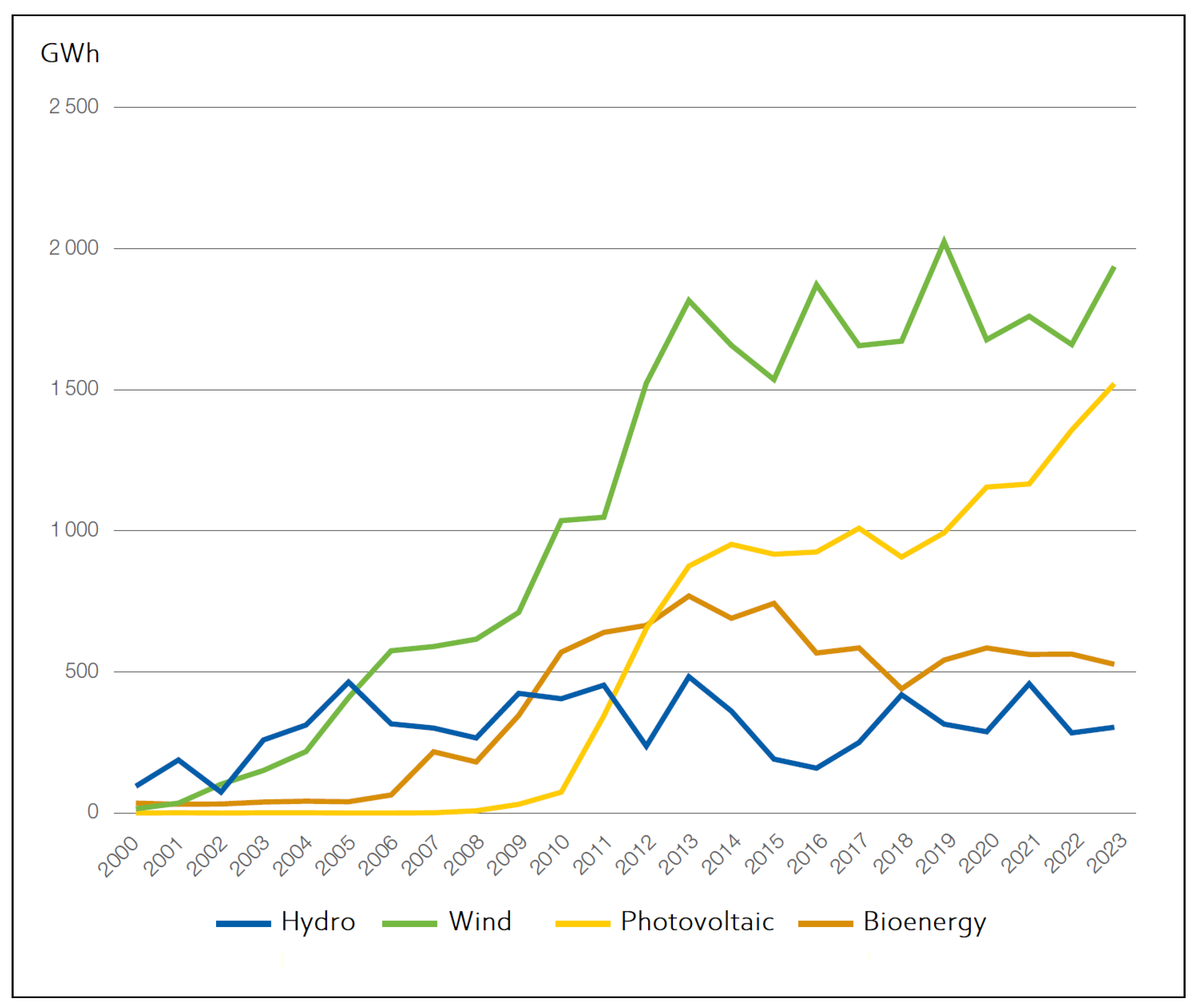
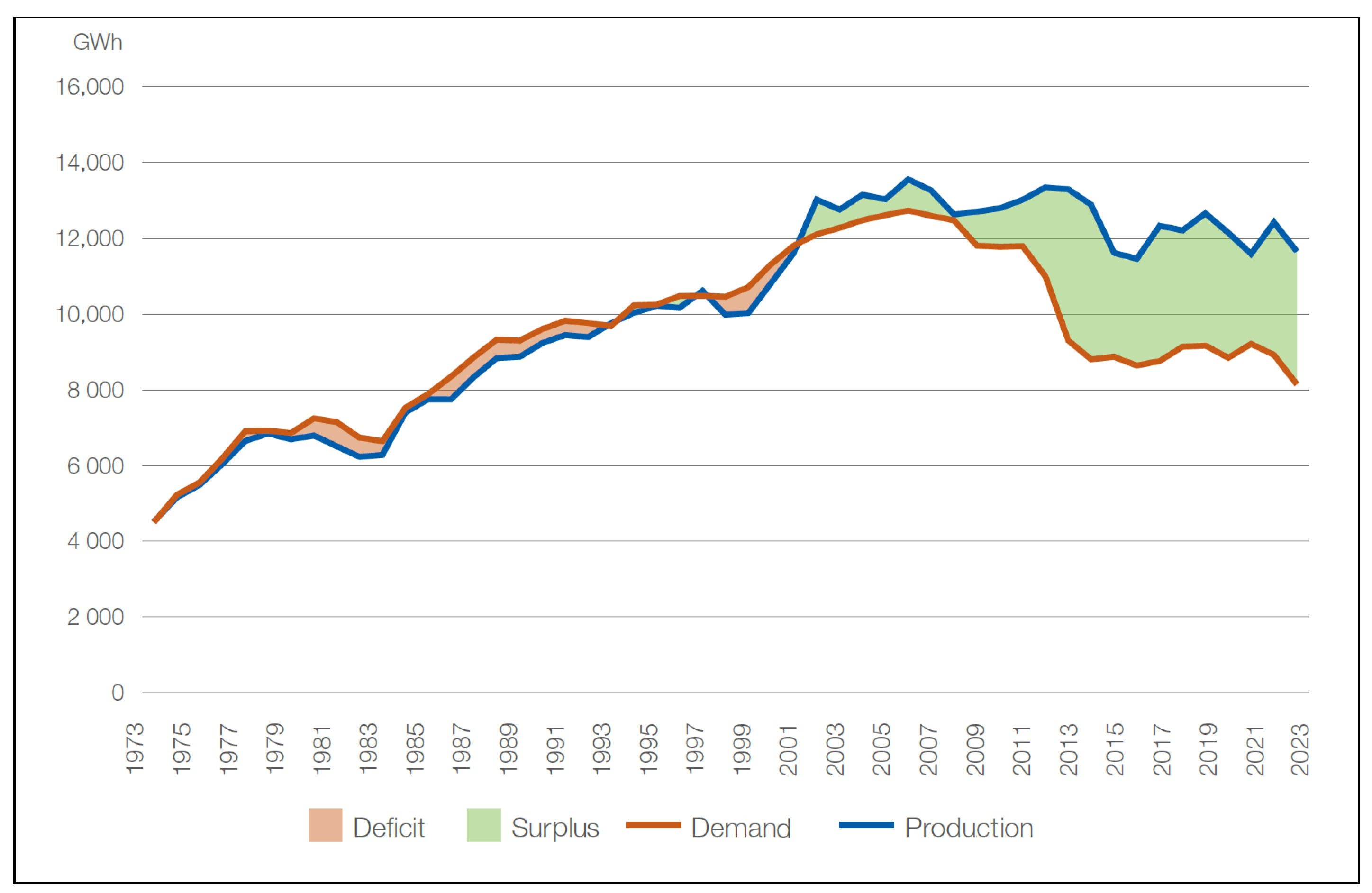
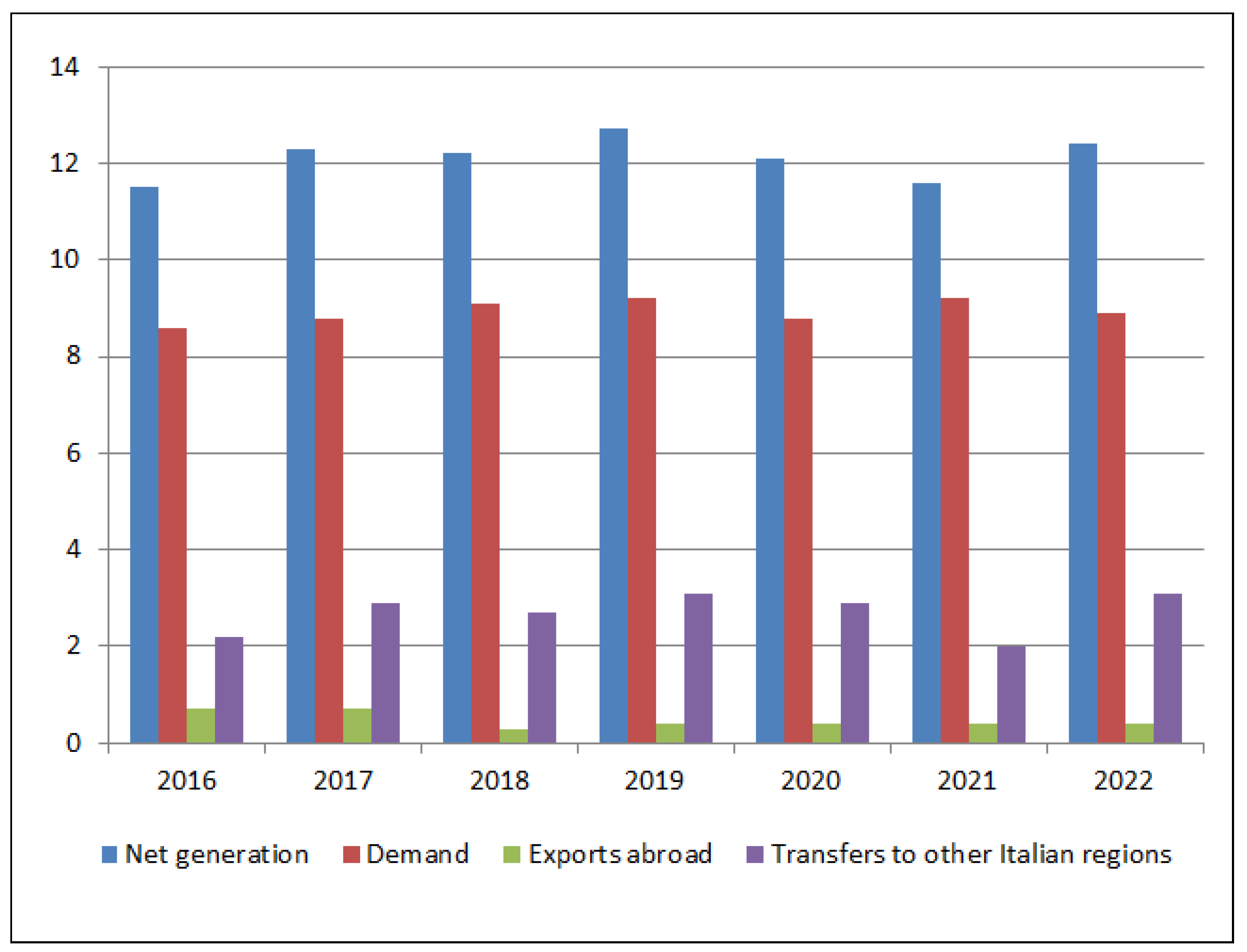
reports gross electricity generation by plant type for 2016–2022 (GWh). Figure A3 depicts gross renewable generation by source for 2000–2022. Figure A4 shows annual production surpluses and deficits relative to demand from 1973 to 2022. Finally, Figure A5 illustrates how net generation was allocated among internal demand, exports abroad, and transfers to other Italian regions during 2016–2022.

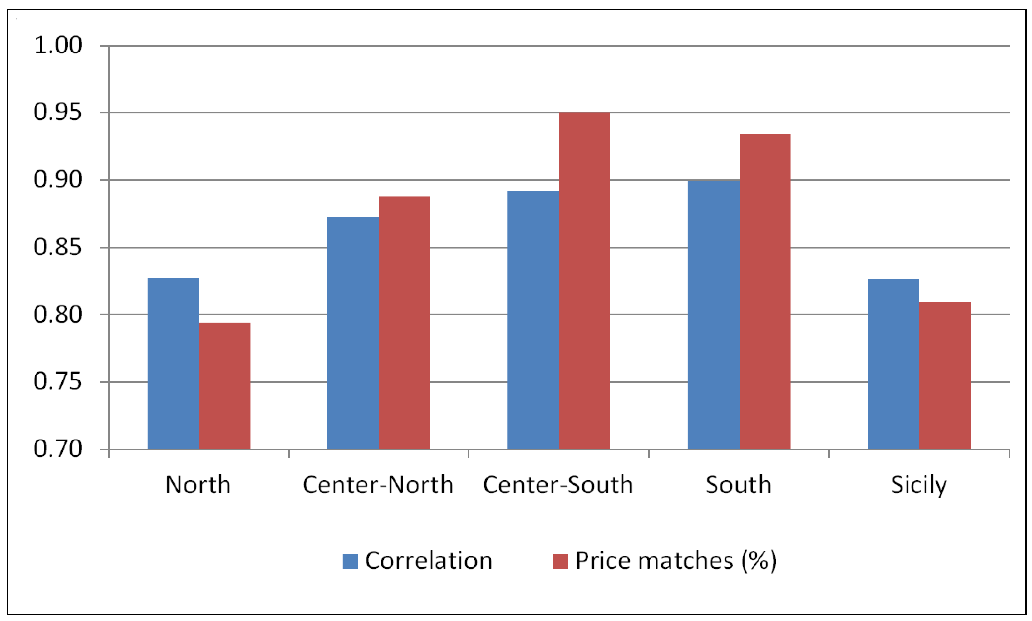
Price statistics in Figure 7 confirm the strong coupling between Sardinia and the rest of Italy. In 2024, the Sardinian zonal day-ahead price matched that of mainland Italian zones in 79–95% of hourly auctions, depending on the zone, and the Pearson correlation between Sardinian prices and mainland Italy prices ranged from 0.83 to 0.90. Such high concordance indicates that arbitrage opportunities identified in Sardinia are representative of those available in the wider Italian market.

Namely, Sardinia recorded identical prices with the Center–South and South bidding zones in 95% and 93% of the hours, respectively, with correlation coefficients that are very close to perfect correlation. Together, these two zones encompass nearly 20 million inhabitants (about one-third of Italy’s population), so the findings from the Sardinian case study would be virtually identical if price data from these zones were used instead.

The relevance extends further because Italy participates in the pan-European single day-ahead market coupling, where prices for all bidding zones are calculated using a common optimization algorithm. Consequently, forecasting models that perform well in the Sardinian context are expected to retain their relative ranking under the same market design elsewhere in Europe. Our results therefore provide insights not only for storage operators active in Italy but also for those participating in the broader integrated European electricity market.

Looking to the future, changes in regulation, market design and network policy are likely to influence the profitability of battery energy storage systems (BESS) by affecting intraday price volatility, the main determinant of arbitrage revenue. Greater penetration of non-dispatchable renewables may widen peak–off-peak spreads (as shown by Macedo et al. [50,51] for southern Europe), whereas measures that strengthen inter-zonal and cross-border interconnections or harmonize market coupling can damp these spreads by exporting surpluses and importing deficits. The Iberian Peninsula’s persistent transmission bottlenecks (which some analyses [52] link to the nationwide blackout of 28 April 2025 affecting both mainland Portugal and peninsular Spain) illustrate how improved transfer capacity could moderate the local price swings that currently create lucrative arbitrage windows. A growing fleet of BESS itself will also provide balancing services that smooth short-term price fluctuations, gradually eroding the very spreads on which arbitrage relies.

Our simulation results nonetheless indicate that whatever volatility regime emerges, operators who base their schedules on price forecasts produced by our top-ranked model (hourly-specified univariate SSA) will capture the highest share of economic value. Because SSA consistently outperforms alternative forecasters across both low and high volatility scenarios tested in this study, it offers BESS operators a robust decision tool under changing regulatory and market conditions.

6.4. Practical Applicability

The evidence presented in this study extends well beyond academic interest and can guide concrete decisions by market participants, policy makers, and system modelers.

Regulatory and investment decisions. Our profit-based evaluation demonstrates that forecast quality converts directly into additional revenue. Regulators can draw on these results when designing tariff mechanisms or market rules that reward accurate bidding, thereby incentivizing information-rich participation, while investors can use the quantified gains to refine business cases and shorten pay-back periods for new battery projects.

Model selection for storage developers. The profitability hierarchy offers clear guidance on which forecasting engines to deploy in real-time operation. A computationally intensive SSA captures nearly the entire profit achievable under perfect foresight, yet parsimonious alternatives such as a 30-day simple moving average still recover about 90% of that value at negligible computational cost. This transparency enables developers to balance computational burden, implementation risk, and expected revenue when scaling fleets across diverse markets.

Integration into Multi-Agent Energy Systems (MAES). The joint price forecasting and bidding optimization framework can provide a reproducible benchmark for MAES researchers and practitioners. Comprehensive reviews on this topic are proposed by Saini et al. [53] and Izmirlioglu et al. [54]; for recent contributions, see also Ding et al. [55]. By mapping forecast accuracy onto explicit market pay-offs, it enables reward functions that reflect true economic value, facilitating rigorous tests of cooperative or competitive dispatch among heterogeneous agents.

Relevance to Integrated Electricity–Heat Systems (IEHS). Integrated electricity–heat systems provide district-heating networks with combined heat and power (CHP) plants and are common in Nordic welfare states, several post-socialist countries, and South Korea (for a review, see [56]; for recent contributions see [57,58,59,60]). Such configurations provide thermal flexibility that lowers intraday electricity-price volatility [61,62,63]. Although lower volatility can compress arbitrage spreads and reduce battery margins, our simulations indicate that accurate SSA-based forecasting can offset this drawback: in our experiment, even during low-volatility periods (such as in 2020), batteries scheduled with SSA captured nearly the full profit potential, whereas simpler models still achieved about 90%. Embedding the same forecast-bidding framework in IEHS optimization tools could enable joint scheduling of thermal and electrical assets, sustain battery profitability, and add additional balancing capacity to the integrated system.

System-level impacts. As batteries become more bankable, wider deployment can itself moderate electricity price swings, facilitate higher renewable shares, and accelerate the energy-transition agenda. Better price forecasting amplifies these benefits by improving revenues at the project level while simultaneously increasing flexibility and resilience across the system.

7. Conclusions

We developed an integrated evaluation framework that couples day-ahead price forecasting with an optimization algorithm that schedules battery charge and discharge to maximize arbitrage revenue. By embedding each forecasting model in the same profit-maximizing framework, we quantified, under identical market and battery constraints, the economic value that every predictive method can deliver. This design provides a consistent basis for ranking forecasting tools according to realized rather than purely statistical performance.

We found that among the forecasting models evaluated, univariate singular spectrum analysis (SSA) consistently yielded the highest arbitrage profits for battery energy storage systems operating in day-ahead electricity markets. Across the five-year horizon from 2020 to 2024, SSA achieved average realized profits equal to 98% of the theoretical maximum, with annual values never falling below 97%. These results were obtained under the assumption of a 4 MWh storage system with a 1 MWh per hour charge–discharge power limit and confirm the effectiveness of SSA in capturing dominant price dynamics with minimal loss of arbitrage value. The SSA implementation exploited the full price history up to the day before bidding, with parameters independently optimized for each hour of the day. These gains, however, came at a steep computational price: the SSA routine demanded processing resources at least an order of magnitude greater than those required by any other forecasting method considered.

While SSA proved the most effective, the simulation results also revealed a second tier of models with strong and relatively consistent performance. This group included the simple 30-day moving average, the “modal” ARIMA and SARIMA configurations, and the “global” random forest with daily retraining over a 3-year rolling window. These approaches achieved average profits between 87.8% and 90.5% of the perfect-foresight benchmark (see Table 3 and Table 10). Their success underscores a key secondary finding: increased model complexity does not necessarily lead to improved financial outcomes. On the contrary, several simpler or more generalized forecasting strategies, such as modal parametrizations or pooled regressors, performed comparably or better than more granular, hour-specific alternatives. The hourly random forest model, for instance, achieved better accuracy (i.e., lower RMSE scores) than its global counterpart but consistently produced lower profits, likely due to its reduced ability to capture primary market characteristics (price oscillations, intraday price ordering, and local extrema) that ultimately inform optimal buy-and-sell decisions. Likewise, increasing the number of trees and the training window length in daily random forest variants had little financial benefit, while incurring substantial computational costs.

The robustness of these findings was verified under three separate modifications to the experimental set-up. First, increasing the charge–discharge power from 1 MWh to 2 MWh per hour, while holding energy capacity constant, had no material effect on the profit hierarchy. Second, switching from annual to daily retraining in the global random forest framework produced only modest improvements. Third, we analyzed the sensitivity to battery-specific costs and found that incorporating realistic battery-efficiency degradation, operation-and-maintenance charges, and transaction fees did not change the ranking. In all cases, the relative performance of the models remained stable, and SSA retained its lead.

These results carry practical implications for energy-market participants. While SSA offers unmatched forecasting precision and profit generation, operational simplicity and scalability also matter. Forecasting models based on simple moving averages or pooled ARIMA/SARIMA parametrizations, and leaner configurations of random forest, offer competitive alternatives with minimal tuning and lower computational demands. From a deployment perspective, these models may be preferred in environments where resource constraints, interpretability, or speed are critical.

In conclusion, our analysis shows that SSA not only surpasses the forecasting accuracy of standard statistical and machine-learning techniques, as documented in the literature [28], but also maximizes battery arbitrage profits when paired with a bidding-optimization framework—a contribution first demonstrated in this study. Nevertheless, simpler forecasting strategies remain remarkably effective, indicating that the pursuit of greater model complexity should be balanced against considerations of operational efficiency and robustness in real-world trading environments.

The implications of these findings extend beyond their academic contribution. They provide regulators and investors with empirical evidence that superior forecasting tools yield tangible economic gains. Improved price predictions strengthen the business case for battery energy storage systems by shortening payback periods and encouraging wider deployment. An expanded storage fleet can then dampen price volatility and supply the flexibility required to accommodate higher shares of variable renewable generation, thus advancing market efficiency, accelerating decarbonization, and ultimately benefiting consumers as well as the broader energy-transition agenda.