A Data-Driven Iterative Feedforward Tuning Strategy with a Variable-Gain Feedback Controller for Linear Servo Systems

Abstract

Iterative feedforward tuning (IFFT) compensates for the dynamic tracking error in linear servo systems caused by reference trajectory and nonlinear friction. The feedback controller with infinite DC gain makes the steady-state tracking error zero. This paper analyzes the effect of the DC gain of the feedback controller on IFFT and proposes an IFFT strategy with a variable-gain feedback controller. This strategy makes the dynamic tracking error due to Coulomb friction behave as a continuous and easy-to-construct window function, which makes the feedforward basis function vector consistent with the dimensionality of the dynamic tracking error. This strategy improves both the efficiency and accuracy of IFFT compared to IFFT using a fixed-gain feedback controller. The dynamic tracking error is compensated to the maximum extent possible, and the steady-state tracking error is zero. Theoretical verification and experimental results indicate the excellent iterative efficiency and accuracy of IFFT with a variable-gain feedback controller.

1. Introduction

Linear servo systems are widely employed in a range of high-precision numerical control machine tools, photolithography workpiece tables, semiconductor packaging equipment, and other fields due to the fact that they do not use intermediate transmission links during the motion process and have significant advantages, including high acceleration, high speed, high efficiency, and high accuracy [1,2,3]. For a linear servo system, the tracking error, which is the difference between the reference trajectory and the motor output displacement, is a critical performance metric. When the linear motor is moving, the tracking error is the dynamic tracking error. When the linear motor ends its motion to reach a stationary state, the tracking error is the steady-state tracking error. In high-precision motion control scenarios, the system design needs to pursue the zero steady-state tracking error and as little the dynamic tracking error as possible to ensure that the linear servo system has high positioning accuracy capability and good dynamic responsiveness. A feedback controller with infinite DC gain can achieve zero steady-state tracking error. Therefore, the improvement in the displacement tracking accuracy of linear servo systems mainly lies in a reduction in the dynamic tracking error.

The feedforward controller is an effective means of compensating for the dynamic tracking error, which is widely employed in motion scenarios requiring precise tracking performance [4,5,6]. The data-driven feedforward controller parameter tuning, known as iterative feedforward tuning (IFFT), is a method of efficiently estimating the optimal values of the feedforward controller parameters to be tuned on the basis of a deterministic feedforward controller structure [7,8]. This is achieved through iterative experiments. A deterministic feedforward controller structure means that the feedforward basis functions are deterministic. The individual feedforward basis functions form the feedforward basis function vector. IFFT is not contingent on a particular reference trajectory and is inherently adaptive to evolving task trajectories. When the working condition does not change, the tracking error does not change if the feedforward controller parameters are the same. A precise set of feedforward controller parameters can accurately compensate for the corresponding dynamic tracking error, even if the reference trajectory is changed. Furthermore, IFFT does not necessitate specific model information, instead relying on input and output data generated during the iterative experimentation of a closed-loop-based motion system. This provides excellent engineering adaptability [9].

Iterative feedforward tuning (IFFT) consists of two parts: the construction of the deterministic feedforward controller structure and the iterative update algorithm of the feedforward controller parameters. The degree of dimensional matching between the feedforward basis function vector and the dynamic tracking error to be compensated, and the accuracy of the feedforward controller parameters, affect the effectiveness of the feedforward controller in compensating for the dynamic tracking error [10]. Currently, most of the strategies to increase the efficiency and accuracy of IFFT are to design different iterative update algorithms but ignore the feedforward basis function vector. In [11,12], an IFFT method based on the gradient descent method (GD) is proposed. This method completes the optimal search for the minimum value of the cost function, which is directly related to the tracking error, through iterative experiments to obtain the optimal estimation of the feedforward controller parameters [13,14]. In [15,16], the practicality of IFFT based on the gradient descent method is enhanced by integrating a set of instrumental variables (IVs) (derivatives at each level of the reference trajectory) into the cost function. In [17], an IFFT method with an adaptive learning step is proposed, which breaks the trade-off between fast convergence and high robustness of existing methods. In [18], a feedforward tuning algorithm based on the heuristic method, self-adaptive hybrid self-learning TLBO, is proposed, which has certain robustness to the initial value and high performance. Improvements in the iterative update algorithm can increase the efficiency and accuracy of IFFT [19,20,21]. But it is indubitable that complex iterative tuning algorithms occupy a larger quantity of memory and have poor scalability in applications [22]. Least squares (LS) is the most universal iterative tuning algorithm due to its simplicity and flexibility [23,24,25]. The gradient method is the most commonly used iterative update algorithm. Both have the step of taking derivatives during the iterative calculation process.

In linear servo systems, in addition to the reference trajectory, nonlinear friction is also an important factor causing motor displacement error [26,27,28,29,30]. More critically, the DC gain of the feedback controller affects the order of the tracking error components [20], which affects the construction of the feedforward basis function vector. The feedback controller with infinite DC gain makes the steady-state tracking error zero. However, it also makes the dynamic tracking error due to Coulomb friction behave as a Dirac function with high pulse amplitude. The feedforward basis function corresponding to this dynamic tracking error term is difficult to construct. And IFFT has a derivative singularity in the meantime. Singularity leads to drastic changes in the direction of the derivative, and it is sensitive to noise and initial values. Small perturbations may lead to completely different directions of updating the feedforward controller parameters. This leads to poor speed and accuracy of IFFT.

To accurately compensate for the dynamic tracking error in linear servo systems caused by reference trajectory and nonlinear friction and ensure the zero steady-state tracking error, this paper proposes an IFFT method with a variable-gain feedback controller. This strategy makes the tracking error due to Coulomb friction behave as a continuous and derivable rectangular window function, which constructs a dimensionally matched feedforward basis function vector. This can quickly and accurately compensate for the dynamic tracking error caused by the reference trajectory and nonlinear friction, and the steady-state tracking error is zero, which improves the working efficiency and positioning motion accuracy of the linear servo system. Particularly, compared to IFFT with a complex and less scalable iterative update algorithm, the strategy proposed in this paper can improve the efficiency and accuracy of compensating for the dynamic tracking error from the design of the construct by simply adjusting the feedback controller.

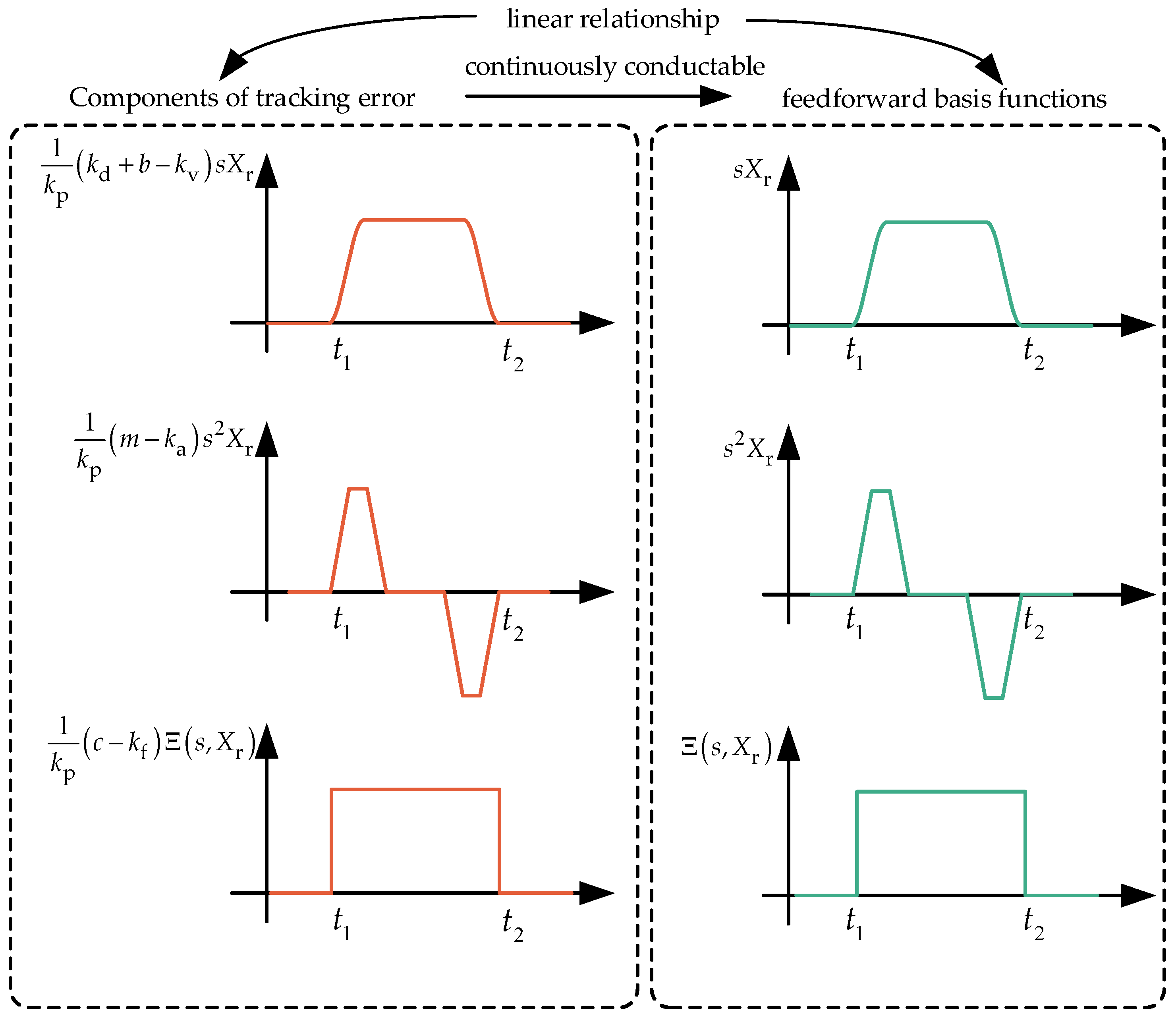
2. Analysis of the Tracking Error of the Linear Servo System

Figure 1 illustrates ‘feedforward + PID feedback’ two-degrees-of-freedom control architecture for linear servo systems. x_r is the reference trajectory. x_m is the motor output displacement. e is the tracking error. u_fb is the feedback controller output. u_ff is the feedforward controller output. T_d is the nonlinear friction [27,28]. f_e is electromagnetic thrust. F(K) is the feedforward controller. K is the feedforward controller parameters matrix. The feedback controller contains G_c1 and G_c2. To increase the response speed and robustness of the system, the differential link of the PID feedback controller (G_c2) is usually set in the feedback loop. The input of the differential link of the PID feedback controller (G_c2) is the motor output displacement.

$$G_{\mathrm{c}1}\left(s\right)=k_{\mathrm{p}}+k_{\mathrm{i}}/s, G_{\mathrm{c}2}\left(s\right)=k_{\mathrm{d}}s$$

(1)

where k_p, k_i, and k_d are the proportional gain coefficients, integral gain coefficients, and differential gain coefficients of the feedback controller.

Without taking into account the force ripple due to the cogging and end effects of the linear motor, the linear servo system dynamics model time domain expression is

$$m{{\mathrm{d}}^2{x}_{\mathrm{m}}\left(t\right)/\mathrm{d}t}^2=f_{\mathrm{e}}\left(t\right)+T_{\mathrm{d}}\left(t\right)$$

(2)

$$T_{\mathrm{d}}\left(t\right)=-b\cdot \mathrm{d}{x}_{\mathrm{m}}\left(t\right)/\mathrm{d}t-c\cdot \mathrm{sgn}\left[\mathrm{d}{x}_{\mathrm{m}}\left(t\right)/\mathrm{d}t\right]$$

(3)

where m is the sum of the mass of the motor and the load. b is the viscous damping coefficient. c is the Coulomb friction coefficient. sgn (•) is the sign function.

$$\mathrm{sgn}\left(x\right)=\left\{\begin{array}{c}1,x>0\\ 0,x=0\\ -1,x<0\end{array}\right.$$

(4)

According to (2), the transfer function G_p of linear motor output displacement and electromagnetic thrust is expressed as

$$G_{\mathrm{p}}\left(s\right)=\mathcal{L}[x_{\mathrm{m}}(t)]/\mathcal{L}[f_{\mathrm{e}}(t)]=1/\left(m{s}^2\right)$$

(5)

where $\mathcal{L}$(·) is the Laplace transform operator.

According to (3), the frequency domain expression of the nonlinear friction is

$$T_{\mathrm{d}}\left[s,X_{\mathrm{m}}\left(s\right)\right]=-bs{X}_{\mathrm{m}}-c\mathsf{\Xi }\left(s,X_{\mathrm{m}}\right)$$

(6)

where X_m is the frequency domain expression of the motor displacement x_m and Ξ(•) is the Laplace transform of the sign function sgn (•) [31].

According to Figure 1, the frequency domain expression of the motor output displacement is

$$X_{\mathrm{m}}\left(s\right)=S\left(G_{\mathrm{c}1}+F\right)X_{\mathrm{r}}+S{T}_{\mathrm{d}}$$

(7)

where X_r is the frequency domain expression of the reference trajectory. S is the input perturbation sensitivity function. Its expression is given by

$$S=G_{\mathrm{p}}{\left(1+G_{\mathrm{p}}{G}_{\mathrm{c}1}+G_{\mathrm{p}}{G}_{\mathrm{c}2}\right)}^{-1}$$

(8)

Combining (1) and (5), the frequency domain expression of the tracking error is

$$E\left(s\right)=X_{\mathrm{r}}-X_{\mathrm{m}}=S\left(G_{\mathrm{c}2}+G_{\mathrm{p}}^{-1}-F\right)X_{\mathrm{r}}-S{T}_{\mathrm{d}}$$

(9)

For a linear servo system with high response characteristics, the speed of the reference trajectory and the motor output speed are approximately equal. sX_m(s) ≈ sX_r(s). Ξ(s, X_m) ≈ Ξ(s, X_r). Therefore, the tracking error e is

$$E(s)=S\left[\left(k_{\mathrm{d}}+b\right)s{X}_{\mathrm{r}}+m{s}^2{X}_{\mathrm{r}}+c\mathsf{\Xi }\left(s,X_{\mathrm{r}}\right)-F{X}_{\mathrm{r}}\right]$$

(10)

When the linear motor is moving, the tracking error is the dynamic tracking error. When the linear motor ends its motion to reach a stationary state, the tracking error is the steady-state tracking error. A feedback controller with infinite DC gain makes the steady-state tracking error zero. Therefore, we need to reduce the dynamic tracking error by IFFT additionally.

3. The Process of Iterative Feedforward Tuning

IFFT consists of two parts: the design of the construct and the iterative update algorithm. The design of the construct involves constructing the feedforward basis function vector. The iterative update algorithm is used to update the feedforward controller parameters. By constructing a feedforward basis function vector that matches the dimension of the dynamic tracking error and tuning the precise feedforward controller parameters, IFFT makes the dynamic tracking error in the linear servo system zero.

Firstly, the feedforward basis function vector in IFFT needs to be constructed. According to (10), in order to match the dimensions of the tracking error, the frequency domain expression of the output of the parametric feedforward controller is

$$\begin{array}{cc}\hfill U_{\mathrm{ff}}(s)& =F(K)X_{\mathrm{r}}(s)=\mathit{\phi }\mathit{K}\hfill \\ & =K_{\mathrm{v}}s{X}_{\mathrm{r}}+K_{\mathrm{a}}{s}^2{X}_{\mathrm{r}}+K_{\mathrm{f}}\mathsf{\Xi }\left(s,X_{\mathrm{r}}\right)\hfill \end{array}$$

(11)

Therefore, the basis function vector φ is

$$\phi =[s{X}_{\mathrm{r}},s^2{X}_{\mathrm{r}},\mathsf{\Xi }\left(s,X_{\mathrm{r}}\right)]$$

(12)

The basis functions include sX_r, s²X_r, and Ξ[s,X_r(s)]. At this point, the tracking error is expressed as

$$E(s)=S\left[\left(b-K_{\mathrm{v}}\right)s{X}_{\mathrm{r}}+\left(m-K_{\mathrm{a}}\right)s^2{X}_{\mathrm{r}}+\left(c-K_{\mathrm{f}}\right)\mathsf{\Xi }\left(s{X}_{\mathrm{r}}\right)\right]$$

(13)

Next, we scalarize the basis function vector φ and construct the sampling matrix Ψ.

$$\Psi =\left[\begin{array}{ccc}{\Psi }_1& {\Psi }_2& {\Psi }_3\end{array}\right]={\left[\begin{array}{ccc}{\mathsf{\Psi }}_1(1)& {\mathsf{\Psi }}_2(1)& {\mathsf{\Psi }}_3(1)\\ {\mathsf{\Psi }}_1(2)& {\mathsf{\Psi }}_2(2)& {\mathsf{\Psi }}_3(2)\\ ⋮& ⋮& ⋮\\ {\mathsf{\Psi }}_1(n)& {\mathsf{\Psi }}_2(n)& {\mathsf{\Psi }}_3(n)\end{array}\right]}_{n\times 3}$$

(14)

where n is the signal length. Ψ₁, Ψ₂, and Ψ₃ are specifically expressed as

$$\left\{\begin{array}{c}{\mathsf{\Psi }}_1={\delta }_{\mathrm{T}}\left(\mathrm{d}{x}_{\mathrm{r}}/\mathrm{d}t\right)/\max \left[{\delta }_{\mathrm{T}}\left(\left|\mathrm{d}{x}_{\mathrm{r}}/\mathrm{d}t\right|\right)\right]\hfill \\ {\mathsf{\Psi }}_2={\delta }_{\mathrm{T}}\left({\mathrm{d}}^2{x}_{\mathrm{r}}/\mathrm{d}{t}^2\right)/\max \left[{\delta }_{\mathrm{T}}\left(\left|{\mathrm{d}}^2{x}_{\mathrm{r}}/\mathrm{d}{t}^2\right|\right)\right]\hfill \\ {\mathsf{\Psi }}_3=\mathrm{sgn}\left\{{\delta }_{\mathrm{T}}\left(\mathrm{d}{x}_{\mathrm{r}}/\mathrm{d}t\right)/\max \left[{\delta }_{\mathrm{T}}\left(\left|\mathrm{d}{x}_{\mathrm{r}}/\mathrm{d}t\right|\right)\right]\right\}\hfill \end{array}\right.$$

(15)

where δ_T(x) denotes sampling the variable x with period T.

To avoid confusion,

Table 1. The relationship between φ, Ψ, and Ψ.

Symbol	Description
φ	the basis function vector
Ψ	the sampling matrix of the basis function vector
Ψ	the specific sampling data in the sampling matrix of the feedforward basis function vector

shows the relationship between φ, Ψ, and Ψ.

Then, the feedforward controller parameter matrix K is calculated by an iterative update algorithm [23]. The process is as follows [25]:

For a given experimental order j, the jth sampling data of the tracking error is E^j, and the jth data of the feedforward controller parameters matrix is valued as K^j at the time.

The appropriate cost function J is chosen, and the feedforward parameter matrix K is updated by the iterative update algorithm that minimizes the cost function J.

$$\Delta K^j=\arg \underset{\Delta K}{\min }J$$

(16)

where arg min (argument of the minimum) denotes the ΔK^j value that makes the cost function J obtain the minimum value.

The feedforward controller parameters are iteratively updated with the final desired effect as:

$$\left\{\begin{array}{l}{K}_{\mathrm{v}}\to b\\ K_{\mathrm{a}}\to m\\ K_{\mathrm{f}}\to c\end{array}\right.\Rightarrow E_{\mathrm{m}}\left(s\right)\to 0\Rightarrow e\left(t\right)\to 0$$

(17)

After iterative feedforward tuning, the feedforward controller parameters find the optimal solution, and the dynamic tracking error tends to zero.

4. Effect of Feedback Controller DC Gain on Tracking Error in Iterative Feedforward Tuning

According to (10) and (17), for a fixed control object (G_p) and relatively stable operating conditions (T_d), the feedback controller affects the construction of the feedforward basis function vector that should match the dynamic tracking error dimension. Therefore, the effect of the DC gain of the feedback controller on the dynamic tracking error in iterative feedforward tuning is specifically discussed next.

Substituting (1) and (5) into (8), the specific expansion of the input perturbation sensitivity function is obtained as

$$S=s/\left(m{s}^3+k_{\mathrm{d}}{s}^2+s{k}_{\mathrm{p}}+k_{\mathrm{i}}\right)$$

(18)

Since the main signal energy of the reference trajectory is distributed in the low-frequency band, under the different the DC gains of the feedback controller, the input perturbation sensitivity function can be approximated as

$$S\approx \underset{s\to 0}{\lim }S=\left\{\begin{array}{cc}1/k_{\mathrm{p}}\hfill & \underset{s\to 0}{\lim }{G}_{\mathrm{c}1}(s)=\sigma \in {ℝ}^{+}\hfill \\ s/k_{\mathrm{i}}\hfill & \underset{s\to 0}{\lim }{G}_{\mathrm{c}1}(s)=\infty \hfill \end{array}\right.$$

(19)

where $\underset{s\to 0}{\lim }{G}_{\mathrm{c}1}(s)$ is the DC gain of the feedback controller.

Bringing (19) to (13), the frequency domain expression of the tracking error is

$$E(s)=\left\{\begin{array}{ll}(k_{\mathrm{d}}+b-k_{\mathrm{v}})s{X}_{\mathrm{r}}\left(s\right)+(m-k_{\mathrm{a}})s^2{X}_{\mathrm{r}}\left(s\right)+(c-k_{\mathrm{f}})\mathsf{\Xi }\left[s,X_{\mathrm{r}}\left(s\right)\right]/k_{\mathrm{p}}\hfill & \underset{s\to 0}{\lim }{G}_{\mathrm{c}1}(s)=\sigma \in {ℝ}^{+}\hfill \\ s\left[(k_{\mathrm{d}}+b-k_{\mathrm{v}})s{X}_{\mathrm{r}}\left(s\right)+(m-k_{\mathrm{a}})s^2{X}_{\mathrm{r}}\left(s\right)+(c-k_{\mathrm{f}})\mathsf{\Xi }\left[s,X_{\mathrm{r}}\left(s\right)\right]\right]/k_{\mathrm{i}}\hfill & \underset{s\to 0}{\lim }{G}_{\mathrm{c}1}(s)=\infty \hfill \end{array}\right.$$

(20)

According to (20), the DC gain of the feedback controller can be divided into finite σ and infinite ∞ to discuss the influence of the feedback controller on IFFT.

4.1. The DC Gain of the Feedback Controller Is Finite σ

When the DC gain of the feedback controller is finite σ, the tracking error e and the basis function vector are linearly related. Then, the tracking error e can be written as

$$E\left(s\right)=\phi \left(M-K\right)/k_{\mathrm{p}}$$

(21)

where M = [b + k_d,m,c]^T is the system parameters matrix.

As an example of a third-order trajectory, the tracking error terms are displayed in Figure 2. t₁ is the starting moment of the linear motor. t₂ is the stopping moment of the linear motor.

At this point, the linear mapping of the tracking error to the feedforward basis functions makes the components of the tracking error continuously derivable with respect to the feedforward basis functions. The feedforward controller parameters can be calculated iteratively by the gradient method or LS.

However, according to the final value theorem, when the DC gain of the feedback controller is finite σ, the steady-state tracking error is

$$\underset{t\to \infty }{\lim }e\left(t\right)=\underset{s\to 0}{\lim }sE\left(s\right)=c/k_{\mathrm{p}}$$

(22)

4.2. The DC Gain of the Feedback Controller Is Infinite ∞

When the DC gain of the feedback controller is infinite ∞, the tracking error component rises in order. The velocity feedforward controller parameters in IFFT will become positively correlated with the acceleration, and the acceleration feedforward controller parameters will become positively correlated with the jerk. The ‘rectangular single-pulse’ error function Ξ(s,X_r) brought about by Coulomb friction will become a Dirac delta function. At this time, it is difficult to construct a suitable Dirac delta function as the basis function. We can only construct acceleration and jerk as the basis functions. According to (20), IFFT is a 3D solution problem. The use of a two-dimensional (2D) model will reduce the efficiency and accuracy of IFFT. The whole process is shown in Figure 3.

According to the final value theorem, when the DC gain of the feedback controller is infinite, the steady-state tracking error is

$$\underset{t\to \infty }{\lim }e\left(t\right)=\underset{s\to 0}{\lim }sE\left(s\right)=0$$

(23)

From the above analysis, it can be seen that when the DC gain of the feedback controller is finite, the error components of each order of the tracking error do not rise in order. It is easy and effective to construct the corresponding feedforward basis function vector (3D) to solve the tracking error minimization problem (3D). But the linear servo system steady-state tracking error is not zero. When the DC gain of the feedback controller is infinite, the steady-state tracking error of the linear servo system is zero. But the error components of the tracking error rise in order. Only a 2D feedforward basis function vector can be constructed to solve the tracking error minimization problem in 3D, which reduces the efficiency and accuracy of IFFT.

5. Iterative Feedforward Tuning with the Variable-Gain Feedback Controller

5.1. Iterative Feedforward Tuning with the Variable-Gain Feedback Controller

Based on the analysis of the tracking error under the different the DC gains of the feedback controller on IFFT, in order to efficiently and completely construct the feedforward basis function vector (3D), which enables IFFT to quickly and accurately reduce the dynamic tracking error (3D) caused by the reference trajectory and nonlinear friction and ensures that the steady-state tracking error is zero, this paper proposes a data-driven IFFT strategy with a variable-gain feedback controller. The overall framework is shown in Figure 4.

In Figure 4, controller C is a controller with fixed gain, which contains k_p and k_d. Controller L is a controller with variable gain k_i. In order to avoid friction caused by the motor low-speed crawling and hysteresis-slip self-excited vibration to the gain change mechanism brought about by the interference, the variable gain’s change moment is decided by the motor reference speed v_r. v_max is the maximum value of the motor reference speed. γ is the target value of the integral gain change. The values of k_p, k_d, and γ can be set according to traditional automatic control theory. ε is the critical motor reference speed. t₁ and t₄ are the motion start command time and the motion stop command time of the linear servo system. t₅ is the time of the next motion start command. t₂ (v_r = ε) and t₃ (v_r = ε) are the moments when the integral gain of the feedback controller k_i is changed.

At the moment t₂, k_i changes from γ to 0, and the DC gain of the feedback controller is changed from infinite to finite. At the moment t₃, k_i changes from 0 to γ, and the DC gain of the feedback controller is changed from finite to infinite. The specific expression of k_i is

$$k_{\mathrm{i}}(t)=\left\{\begin{array}{l}\gamma \mathrm{sech}\left[\alpha \left(t-t_1\right)\right],t\in \left[t_2,t_3\right]\\ \gamma -\gamma \mathrm{sech}\left[\alpha \left(t-t_2\right)\right],t\in \left[t_3,t_5\right]\\ \gamma ,\mathrm{otherwise}\end{array}\right.$$

(24)

where sech(x) = 2/(e^αx + e^−αx). α determines the rate of change of the integral gain k_i.

According to (20) and (24), when ε is small enough, the tracking error is

$$E\left(s\right)=\left\{\begin{array}{cc}\phi \left(M-K\right)/k_{\mathrm{p}}& \left|v_{\mathrm{r}}(t)\right|\ge \epsilon \\ 0& \left|v_{\mathrm{r}}(t)\right|<\epsilon \end{array}\right.$$

(25)

The tracking error E(s) exists linearly in the subspace Ψ formed by the basis function vector φ = [sX_r, s²X_r, Ξ(s,X_r)].

That is, under the action of the variable-gain feedback controller, the feedforward basis function vector (3D) can be constructed simply and efficiently. The feedforward compensation dimension is the same as the tracking error dimension (3D), which increases the efficiency and accuracy of IFFT. This results in a linear servo system with well-compensated dynamic tracking error and zero steady-state tracking error.

The IFFT process with the variable-gain feedback controller is as follows:

Remember the iteration order as j. Sampling the tracking error for n times, the jth sampling of the tracking error is

$$E^j={\left[\begin{array}{cccc}{E}_{\mathrm{m}}\left(1\right)& E_{\mathrm{m}}\left(2\right)& \dots & E_{\mathrm{m}}\left(n\right)\end{array}\right]}_{n\times 1}^{\mathrm{T}}$$

(26)

Using the sum of squared residuals as the cost function, the minimization problem of the tracking error with ‘e = 0’ is constructed as

$$\Delta K^j=\arg \underset{\Delta K}{\min }{‖\Psi \Delta K^j-E_{\mathrm{m}}^j‖}_2$$

(27)

Based on the linear mapping of the tracking error to the feedforward basis function vector φ, (27) has a least squares solution of

$$\Delta K^j={\left({\Psi }^{\mathrm{T}}\Psi \right)}^{-1}{\Psi }^{\mathrm{T}}{E}_{\mathrm{m}}^j$$

(28)

At this point, the iterative update algorithm of the feedforward controller parameters matrix is

$$K^{j+1}=K^j+\chi \Delta K^j$$

(29)

where χ is the iteration step matrix. The amplitude of the iteration step determines the rate of change of the feedforward controller parameter. An optimal iteration step matrix can be calculated in a pre-experiment using the least squares method with an initial value of diag [1,1,1].

The expansion of (27) is

$$\begin{array}{cc}\hfill K^{j+1}& =K^j+\chi {\left({\Psi }^{\mathrm{T}}\Psi \right)}^{-1}{\Psi }^{\mathrm{T}}{E}_{\mathrm{m}}^j\hfill \\ & =\left[I-{\displaystyle \frac{1}{k_{\mathrm{p}}}}\chi {\left({\Psi }^{\mathrm{T}}\Psi \right)}^{-1}{\Psi }^{\mathrm{T}}\phi \right]K^j+{\displaystyle \frac{1}{k_{\mathrm{p}}}}\chi {\left({\Psi }^{\mathrm{T}}\Psi \right)}^{-1}{\Psi }^{\mathrm{T}}\phi M\hfill \end{array}$$

(30)

At this point,

$$\left|I-{\displaystyle \frac{1}{k_{\mathrm{p}}}}\chi {\left({\Psi }^{\mathrm{T}}\Psi \right)}^{-1}{\Psi }^{\mathrm{T}}\phi \right|<1$$

(31)

During the update of the feedforward parameter matrix, (31) satisfies the convergence condition of Banach’s immovable point theorem (contraction mapping theorem). Therefore, the result of IFFT is

$$\left\{\begin{array}{l}\underset{j\to \infty }{\lim }{K}^j\to M\\ \underset{j\to \infty }{\lim }{E}^j\to \overrightarrow{0}\end{array}\right.$$

(32)

Finally, according to Parseval’s theorem, the tracking error tends to zero in the time domain.

In summary, the variable-gain feedback controller makes the feedforward basis function vector (3D) consistent with the dynamic tracking error (3D) in dimension. The dynamic tracking error minimization problem is three linear equations. At this point, the optimal feedforward controller parameter matrix is obtained by fast iteration in the least-squares closed-form solution, which finally makes the dynamic tracking error tend to zero. At the same time, the steady-state tracking error is zero.

5.2. The Proof of the Stability of a System with the Variable-Gain Feedback Controller

The change in integral gain in the feedback controller makes the whole motion control system a variable-gain feedback control system, as shown in Figure 3. u is the output of the controller L. The tracking error can be written as

$$E\left(s\right)=G_{\mathrm{er}}{X}_{\mathrm{r}}-G_{\mathrm{eu}}\left(u+T_{\mathrm{d}}\right)$$

(33)

where $G_{\mathrm{er}} = S\left(G_{\mathrm{p}}^{-1} + {\mathrm{G}}_{\mathrm{c}2} - F\right), G_{\mathrm{eu}} = S$

$$G_{\mathrm{er}} = S\left(G_{\mathrm{p}}^{-1} + {\mathrm{G}}_{\mathrm{c}2} - F\right), G_{\mathrm{eu}} = S$$

The corresponding state space equation of (33) can be expressed as

$$\left\{\begin{array}{l}\mathrm{d}{x}_{\mathrm{e}}/\mathrm{d}t=A_{\mathrm{e}}{x}_{\mathrm{e}}-B_{\mathrm{e}1}u+B_{\mathrm{e}2}d\\ e=C_{\mathrm{e}}{x}_{\mathrm{e}}+D_{\mathrm{e}}d\end{array}\right.$$

(34)

where the state vector x_e = [x_m,dx_m/dt]^T ∈ ℝ^2×1, with additional variable gain control inputs u ∈ ℝ. The external input is d = [x_r,T_d] ^T ∈ ℝ^2×1. The output vector is the tracking error e ∈ ℝ. The system matrix A ∈ ℝ^2×2 is a Hurwitz matrix. B_e1 ∈ ℝ^2×1. B_e2 ∈ ℝ^2×2. C_e ∈ ℝ^1×2. D_e = [1,−1]. (A_e, B_e1, B_e2) are controllable. (A_e, C_e) are observable. And G_eu = C_e(sI − A_e)⁻¹B_e1.

The state space equation of the controller L(s) is given by

$$\left\{\begin{array}{l}\mathrm{d}{x}_{\mathrm{s}}/\mathrm{d}t=A_{\mathrm{s}}{x}_{\mathrm{s}}+B_{\mathrm{s}}e\\ y_{\mathrm{s}}=C_{\mathrm{s}}{x}_{\mathrm{s}}\end{array}\right.$$

(35)

where the state vector is x_s ∈ ℝ^1×1. The motor displacement tracking error is e ∈ ℝ. The output of the control system with variable gain is y_s ∈ ℝ. And Y(s) = L(s)E(s). The system matrix A_s ∈ ℝ^1×1 is a Hurwitz matrix. B_s ∈ ℝ^1×1. C_s∈ℝ^1×1. L(s) = C_s(sI − A_s)⁻¹B_s.

Based jointly on (34) and (35), the extended state model of the overall variable-gain feedback control system is

$$\left\{\begin{array}{l}\mathrm{d}x/\mathrm{d}t=Ax-B_{1}u+B_{2}d\\ z=Cx+Dd\\ u=\upsilon \varphi \left(z\right)\end{array}\right.$$

(36)

with

$$A=\left[\begin{array}{cc}{A}_{\mathrm{e}}& 0^{2\times 1}\\ B_{\mathrm{s}}{C}_{\mathrm{e}}& A_{\mathrm{s}}\end{array}\right],B_1=\left[\begin{array}{c}{B}_{\mathrm{e}1}\\ 0\end{array}\right],B_1=\left[\begin{array}{c}{B}_{\mathrm{e}2}\\ B_{\mathrm{s}}{D}_{\mathrm{e}}\end{array}\right],C=\left[\begin{array}{cc}{C}_{\mathrm{e}}& 0\\ 0^{1\times 2}& C_{\mathrm{s}}\end{array}\right],D=\left[\begin{array}{c}{D}_{\mathrm{e}}\\ 0\end{array}\right],\upsilon =\left[1,1\right]$$

where the state vector x = [x_e,x_s]^T ∈ ℝ^2×1. The external input is d = [x_r,T_d]^T ∈ ℝ^2×1, with additional variable gain input u ∈ ℝ. The output is z = [e,y_s]^T ∈ ℝ^2×1. (A, B₁, B₂) are controllable and (A, C) are observable.

Then, there is

$$\varphi \left(z\right)=\left\{\begin{array}{l}{\left[\begin{array}{c}\gamma \mathrm{sech}\left[\alpha \left(t-t_1\right)\right]y_{\mathrm{s}}\hspace{1em}0\hfill \end{array}\right]}^{\mathrm{T}},t\in \left[t_2,t_3\right]\hfill \\ {\left[0\hspace{1em}\left\{\gamma -\gamma \mathrm{sech}\left[\alpha \left(t-t_2\right)\right]\right\}{y}_{\mathrm{s}}\right]}^{\mathrm{T}},t\in \left[t_3,t_5\right]\hfill \\ {\left[\begin{array}{cc}0& 0\end{array}\right]}^{\mathrm{T}},\mathrm{otherwise}\hfill \end{array}\right.$$

(37)

According to (37), ϕ(z) is segmentally continuous on t, and local Lipschitz in z, and memoryless ϕ(z) satisfies the sector condition ϕ(z)[ϕ(z) − Hz] < 0. According to (36), the variable-gain system can be expressed as a Lur’e system (shown in Figure 5). This system has a linear constant forward path and a memoryless time-varying nonlinear feedback path. The Lur’e system can be proved to be stable using the circle criterion.

The transfer function from −ϕ(z) to z can be written as

$$T\left(s\right)=C{\left(sI-A\right)}^{-1}{B}_1\upsilon =\left[\begin{array}{cc}{G}_{\mathrm{eu}}& G_{\mathrm{eu}}\\ L{G}_{\mathrm{eu}}& L{G}_{\mathrm{eu}}\end{array}\right]$$

(38)

According to the circle criterion, the variable-gain controller stabilizes the closed-loop system when the transfer function [I + HT] is strictly positive real. Since it is difficult to verify the positive real nature of [I + HT], consider the equivalence of the following expressions based on those in [32].

(1) [I + HT] is strictly positive real.

(2) There exists a matrix P = P^T > 0, such that

$$\left[\begin{array}{cc}PA+A^{\mathrm{T}}P& P{B}_1\upsilon -C^{\mathrm{T}}H\\ {\upsilon }^{\mathrm{T}}{B}^{\mathrm{T}}P-HC& -2I\end{array}\right]<0$$

(39)

The control object G_p is stabilized by the controller C under a uniform bounded reference trajectory x_r and an external perturbation T_d. For a given integral gain k_i, [I + HT] is strictly positive real if the Linear Matrix Inequality (LMI) has a solution for P. Therefore, according to the circle criterion, the variable-gain controller makes the closed-loop system stable.

In summary, the variable-gain feedback controller in this paper requires three parameters, which include the upper limit value of variable integral gain γ, the rate value of the integral gain change α, and the motor reference speed value that triggers integral gain change ε. The choice of γ and α needs to be based on Routh’s criterion and the circle criterion to ensure that the LMI has a solution for P. The choice of ε should be as small as possible to compensate for the dynamic tracking error as much as possible by using IFFT.

6. Experimental Validation

6.1. Introduction of the System Experimental Platform

In order to verify the correctness of the theoretical analyses and the effectiveness of the proposed strategy, a linear motion experimental platform was built, as shown in Figure 6. The experimental platform consisted of a permanent magnet synchronous linear motor (PMLSM), servo controllers (Power Umac), a power amplifier (Servotronix drives), a grating scale, and a displacement sensor. The accuracy of the displacement sensor is 1 µm.

The parameters of the PMLSMs are shown in

Table 2. The parameters of the PMLSMs.

Item	Value	Unit
Rated voltage, Vn	220	V
Rated power, Pn	103.9	W
Thrust constant, KT	10.355	N/A
Action mass, mm	1.1	kg
Limit of current	12	A

.

The parameters of the reference trajectory used in the experiment are shown in

Table 3. The parameters of the reference trajectory used in the experiment.

Reference Trajectory	Maximum Displacement xmax	Maximum Velocity vmax	Maximum Acceleration amax	Maximum Jerk jmax
R1	0.045 (m)	0.2 (m/s)	5 (m/s2)	250 (m/s3)
R2	0.045 (m)	0.3 (m/s)	6 (m/s2)	240 (m/s3)

. The waveform of the reference trajectory is shown in Figure 7. To visualize the linear servo system’s performance, the experiment presents the tracking error waveform.

Based on the variable-gain feedback controller, the critical velocity ε = 1 × 10−5 (m/s) was set in order to compensate for the dynamic error as much as possible by using IFFT. The upper limit value of variable integral gain γ = 2,000,000, and the rate value of the integral gain change α = 100 by Routh’s criterion and the circle criterion. The iteration step matrix χ = diag [180,100,50] was set by a pre-experiment.

6.2. Operational Stability Verification of the System Based on the Variable-Gain Feedback Controller

Figure 8 demonstrates the experimental plot of the motor running speed based on IFFT with a variable-gain feedback controller under different reference trajectories (R1 and R2).

As can be seen in Figure 8, the data-driven IFFT strategy with a variable-gain feedback controller proposed in this paper can operate stably under different reference trajectories.

6.3. Verification of the Tracking Errors with Various Orders of Elevation Under the Action of Feedback Controllers with Different DC Gains

Figure 9 demonstrates the comparison of the experimental waveforms of the tracking error under the feedback controller with finite DC gain and the experimental waveforms of the tracking error under the feedback controller with infinite DC gain under different feedforward parameters (precise K_v, precise K_v,a, and precise K_v,a,f).

In Figure 9a, it can be seen that the dominant term of the dynamic tracking error under the action of the feedback controller with finite DC gain is linearly related to the feedforward basis function. At this time, the dynamic tracking error is continuously derivable with respect to the feedforward basis functions. Moreover, the dynamic tracking error (3D) is dimensionally matched to the feedforward basis function vector (3D). However, when there is nonlinear friction interference, the feedback controller with finite DC gain cannot achieve zero steady-state tracking error.

In Figure 9b, the feedback controller with infinite DC gain acts with zero steady-state tracking error. However, the dominant term of the dynamic tracking error rises in order with respect to the old feedforward basis functions. The new feedforward basis functions need to be constructed. But, at this time, the tracking error due to Coulomb friction corresponds to a feedforward basis function with a Dirac function, which has a high pulse amplitude. It is difficult to construct. The feedforward basis function vector (2D) does not match the tracking error (3D) in dimension.

6.4. Performance Verification of Efficient and Highly Accurate Iterative Feedforward Tuning with the Variable-Gain Feedback Controller

Figure 10 demonstrates the experimental comparison plot of IFFT with the fixed-gain feedback controller and IFFT with the variable-gain feedback controller with the motor running the R1 reference trajectory. The iterative updating algorithm is LS, and the feedforward basis function vector of IFFT with the fixed-gain feedback controller transforms to [s²X_r, s³X_r]^T. In addition, the iterative update algorithm of the gradient descent method (GD) is used as a comparison.

Figure 11 demonstrates the variation in the maximum value of the tracking error e_max during IFFT with the fixed-gain feedback controller and the variable-gain feedback controller. The iterative update algorithm of the gradient descent method (GD) is used as a comparison.

Figure 12 demonstrates the variation in the non-zero root mean square value of the tracking error e_nrms during IFFT with the fixed-gain feedback controller and the variable-gain feedback controller. The iterative update algorithm of the gradient descent method (GD) is used as a comparison.

Table 4. The numerical variation of the maximum value of the tracking error e_max.

Number of iterations	IFFT with the Fixed-Gain Feedback Controller (LS) (µm)	IFFT with the Fixed-Gain Feedback Controller (GD) (µm)	IFFT with the Variable-Gain Feedback Controller (LS) (µm)
1	291.95	292.24	619.97
2	237.86	238.65	158.13
3	232.87	232.04	39.64
4	208.47	181.14	13.83
5	168.45	143.52	8.00
···	···	···	···
30	11.89	11.49	8.00

demonstrates the numerical variation in the maximum value of the tracking error e_max during IFFT with the fixed-gain feedback controller and the variable-gain feedback controller. The iterative update algorithm of the gradient descent method (GD) is used as a comparison.

Table 5. The numerical variation in the non-zero root mean square value of the tracking error e_nrms

Number of iterations	IFFT with the Fixed-Gain Feedback Controller (LS) (µm)	IFFT with the Fixed-Gain Feedback Controller (GD) (µm)	IFFT with the Variable-Gain Feedback Controller (LS) (µm)
1	113.98	113.84	443.28
2	91.55	91.40	105.093
3	82.03	76.20	23.40
4	68.25	63.21	5.54
5	58.64	52.93	2.79
···	···	···	···
30	4.23	3.83	2.74

demonstrates the numerical variation in the non-zero root mean square value of the tracking error e_nrms during IFFT with the fixed-gain feedback controller and the variable-gain feedback controller. The iterative update algorithm of the gradient descent method (GD) is used as a comparison.

Based on Figure 10, Figure 11 and Figure 12 and Table 4 and Table 5, IFFT with the variable-gain feedback controller requires five iterations to reach the best performance. IFFT with the fixed-gain feedback controller under LS requires 30 iterations to reach the best performance. IFFT with the fixed-gain feedback controller under the gradient descent method requires 20 iterations to reach the best performance. In terms of the maximum tracking error and the non-zero root mean square of the tracking error, the result of IFFT with the variable-gain feedback controller (e_max = 8.00 µm, e_nrms = 2.74 µm) is better than IFFT with the fixed-gain feedback controller under LS (e_max = 11.89 µm, e_nrms = 4.23 µm) and IFFT with the fixed-gain feedback controller under the gradient descent method (e_max = 11.49 µm, e_nrms = 3.83 µm). That is, the efficiency of IFFT with the variable-gain feedback controller is improved by 83%, and the accuracy is improved by 35%, compared to IFFT with the fixed-gain feedback controller under LS. The efficiency of IFFT with the variable-gain feedback controller is improved by 75%, and the accuracy is improved by 28%, compared to IFFT with the fixed-gain feedback controller under the gradient descent method. The dynamic tracking error is compensated to the maximum extent possible, and the steady-state tracking error is zero.

6.5. Verification of Trajectory Adaptation of Iterative Feedforward Tuning Results

Figure 13 shows the waveforms of the tracking error for the motor running the R1 and R2 reference trajectories using the feedforward controller parameters that were rectified under R1.

In Figure 13, when the motor runs the R1 trajectory, the maximum value of the tracking error e_max is 8.00 μm, and the non-zero root mean square value of the tracking error e_nrms is 2.74 μm. When the motor runs the R2 trajectory, the maximum of the tracking error e_max is 6.21 μm, and the non-zero root mean square value of the tracking error e_nrms is 2.58 μm. As can be seen in Figure 11, the iterative feedforward calibration parameters have good trajectory adaptability for the same operating conditions. A precise set of feedforward controller parameters can accurately compensate for the corresponding dynamic tracking error, even if the reference trajectory is changed.

7. Conclusions

In this paper, based on the control framework of a ‘feedforward + feedback’ linear servo system, the influence of the DC gain of the feedback controller on IFFT is analyzed:

(a) When the DC gain of the feedback controller is finite, the tracking error consists linearly of velocity (the first-order differential terms of the reference trajectory), acceleration (the second-order differential terms of the reference trajectory), and Coulomb friction (the sign function terms determined by the first-order differential terms of the reference trajectory). The feedforward basis functions can be constructed directly and efficiently as follows: velocity, acceleration, and Coulomb friction. The feedforward basis function vector is of the same dimension (3D) as the tracking error. The tracking error can be differentiated with respect to the feedforward basis functions. The feedforward basis functions are dimensionally complete, and the feedforward controller parameters that make the dynamic tracking error zero can be solved accurately by IFFT. But the steady-state tracking error is not zero.

(b) When the DC gain of the feedforward controller is infinite, each error component of the tracking error rises in order. In this case, the dynamic tracking error due to Coulomb friction behaves as a Dirac function with high pulse amplitude. The feedforward basis function corresponding to this error term is difficult to construct. The tracking error in 3D (velocity, acceleration, and Coulomb friction) can only be compensated by a 2D feedforward controller (acceleration and jerk). Thus, the efficiency and accuracy of IFFT are low.

Based on the influence of the DC gain of the feedback controller on IFFT, this paper proposes a data-driven IFFT strategy with a variable-gain feedback controller: when the reference speed is low, the feedback controller has a finite DC gain, and the rest have an infinite DC gain. By using the variable-gain feedback controller, this IFFT strategy constructs a feedforward basis function vector (3D) that matches the tracking error (3D) in dimension simply and efficiently. It solves the problem of dimensional mismatch between the feedforward basis function vector and the tracking error due to the order rise in the tracking error under the infinite DC gain of the feedback controller. This feature improves the efficiency and accuracy of IFFT. The strategy reduces the dynamic tracking error due to the reference trajectory and nonlinear friction as much as possible, and the steady-state tracking error is zero.

References

1. Erwinski, K.; Wawrzak, A.; Paprocki, M. Real-Time Jerk Limited Feedrate Profiling and Interpolation for Linear Motor Multiaxis Machines Using NURBS Toolpaths. IEEE Trans. Ind. Inform. 2022, 18, 7560–7571. [Google Scholar] [CrossRef]
2. Gao, H.; Shi, T.N.; Gao, X.M.; Lei, Y.X.; Yan, D.; Guo, L.Y.; Yan, Y. Electromagnetic characteristic analysis and design of a linear motor used for ultra-high-speed EMS maglev train. Sci. China-Technol. Sci. 2024, 67, 1957–1973. [Google Scholar] [CrossRef]
3. Zhong, Z.M.; Xiao, Q.H.; Wang, X.S.; Yang, M.L.; Wang, Y.Q. Optimal Design of Doubly-Fed Linear Motor for High Speed Maglev Train Based on Improved Genetic Algorithm. In Proceedings of the 2023 IEEE International Conference on Mechatronics and Automation (ICMA), Harbin, China, 6–9 August 2023; pp. 2089–2094. [Google Scholar] [CrossRef]
4. Iwasaki, M.; Seki, K.; Maeda, Y. High-Precision Motion Control Techniques: A Promising Approach to Improving Motion Performance. IEEE Ind. Electron. Mag. 2012, 6, 32–40. [Google Scholar] [CrossRef]
5. Zhou, R.; Hu, C.; Ou, T.; Wang, Z.; Zhu, Y. Intelligent GRU-RIC position-loop feedforward compensation control method with application to an ultraprecision motion stage. IEEE Trans. Ind. Inform. 2023, 20, 5609–5621. [Google Scholar] [CrossRef]
6. Zhou, R.; Hu, C.; Wang, Z.; Zhu, Y.; Tomizuka, M. Real-time iterative compensation control using plant-injection feedforward architecture with application to ultraprecision wafer stage. IEEE Trans. Ind. Inform. 2024, 20, 11708–11719. [Google Scholar] [CrossRef]
7. Li, M.; Zhu, Y.; Yang, K.M.; Yang, L.H.; Hu, C.X. Data-based switching feedforward control for repeating and varying tasks: With application to an ultraprecision wafer stage. IEEE Trans. Ind. Electron. 2019, 66, 8670–8680. [Google Scholar] [CrossRef]
8. Zhao, H.Y.; Li, L.; Liu, Y. Iterative Control Decoupling Tuning by Feedforward Compensation for Precision Motion Stage. In Proceedings of the 2023 IEEE 12th Data Driven Control and Learning Systems Conference, Xiangtan, China, 12–14 May 2023; pp. 1812–1817. [Google Scholar] [CrossRef]
9. Song, F.Z.; Liu, Y.; Xu, J.X.; Yang, X.F.; He, P.; Yang, Z.L. Iterative Learning Identification and Compensation of Space-Periodic Disturbance in PMLSM Systems With Time Delay. IEEE Trans. Ind. Electron. 2018, 65, 7579–7589. [Google Scholar] [CrossRef]
10. Song, F.Z.; Liu, Y.; Xu, J.X.; Yang, X.F.; Zhu, Q. Data-Driven Iterative Feedforward Tuning for a Wafer Stage: A High-Order Approach Based on Instrumental Variables. IEEE Trans. Ind. Electron. 2019, 66, 3106–3116. [Google Scholar] [CrossRef]
11. Meulen, S.V.D.; Tousain, R.; Bosgra, O. Fixed Structure Feedforward Controller Tuning Exploiting Iterative Trials, Applied to a High-Precision Electromechanical Servo System. In Proceedings of the 2007 American Control Conference, New York, NY, USA, 9–13 July 2007; pp. 4033–4039. [Google Scholar] [CrossRef]
12. Xu, H.J.; Hinze, C.; Iannelli, A.; Verl, A. Robust Inversion-Based Feedforward Control with Hybrid Modeling for Feed Drives. IEEE Trans. Control Syst. Technol. 2024, 33, 858–871. [Google Scholar] [CrossRef]
13. Song, F.Z.; Liu, Y.; Dong, Y.; Chen, X.K.; Tan, J.B. Motion Control of Wafer Scanners in Lithography Systems: From Setpoint Generation to Multistage Coordination. IEEE Trans. Instrum. Meas. 2024, 73, 7508040. [Google Scholar] [CrossRef]
14. Fu, X.W.; Yang, X.F.; Zanchetta, P.; Tang, M.; Liu, Y.; Chen, Z.Y. An Adaptive Data-Driven Iterative Feedforward Tuning Approach Based on Fast Recursive Algorithm: With Application to a Linear Motor. IEEE Trans. Ind. Inform. 2024, 19, 6160–6169. [Google Scholar] [CrossRef]
15. Boeren, F.; Oomen, T.; Steinbuch, M. Iterative motion feedforward tuning: A data-driven approach based on instrumental variable identification. Control Eng. Pract. 2015, 37, 11–19. [Google Scholar] [CrossRef]
16. Boeren, F.; Bruijnen, D.; Oomen, T. Enhancing feedforward controller tuning via instrumental variables: With application to nanopositioning. Int. J. Control 2017, 90, 746–764. [Google Scholar] [CrossRef]
17. Song, F.Z.; Liu, Y.; Jin, W.; Tan, J.B.; He, W. Data-Driven Feedforward Learning with Force Ripple Compensation for Wafer Stages: A Variable-Gain Robust Approach. IEEE Trans. Neural Netw. Learn. Syst. 2022, 33, 1594–1608. [Google Scholar] [CrossRef]
18. Chen, S.W.; Liu, Y.; Song, F.Z. Data-driven Rational Feedforward Tuning Algorithm Based on Self-adaptive Hybrid Self-learning TLBO. In Proceedings of the 2023 IEEE 12th Data Driven Control and Learning Systems Conference, Xiangtan, China, 12–14 May 2023; pp. 1516–1632. [Google Scholar] [CrossRef]
19. Dai, L.Y.; Li, X.; Zhu, Y.; Zhang, M. Auto-tuning of model-based feedforward controller by feedback control signal in ultraprecision motion systems. Mech. Syst. Signal Proc. 2020, 142, 106764. [Google Scholar] [CrossRef]
20. Dai, L.Y.; Li, X.; Zhu, Y.; Zhang, M.; Hu, C.X. The Generation Mechanism of Tracking Error During Acceleration or Deceleration Phase in Ultraprecision Motion Systems. IEEE Trans. Ind. Electron. 2019, 66, 7109–7119. [Google Scholar] [CrossRef]
21. Sun, Y.X.; Li, X.Q.; Luo, Y.; Chen, X.D.; Zeng, L.Z. Iterative Tuning of Feedforward Controller with Precise Time-Delay Compensation for Precision Motion System. Math. Probl. Eng. 2020, 2020, 9391526. [Google Scholar] [CrossRef]
22. Li, L.; Liu, Y.; Li, L.Y.; Tan, J.B. Kalman-Filtering-Based Iterative Feedforward Tuning in Presence of Stochastic Noise: With Application to a Wafer Stage. IEEE Trans. Ind. Inform. 2019, 15, 5816–5826. [Google Scholar] [CrossRef]
23. Zhang, X.X.; Li, M.; Yao, X.Y. Data-driven tuning of feedforward controller structured with infinite impulse response filter via iterative learning control. IET Control Theory Appl. 2019, 13, 1062–1070. [Google Scholar] [CrossRef]
24. Dai, L.Y.; Li, X.; Zhu, Y.; Zhang, M. Feedforward tuning by fitting iterative learning control signal for precision motion systems. IEEE Trans. Ind. Electron. 2020, 68, 8412–8421. [Google Scholar] [CrossRef]
25. Liu, M.H.; Wang, M.Y.; Li, J.C.; Sun, Q.W.; Zhang, C.M.; Li, L.Y. Adaptive Feedforward Control Based on Recursive Least Squares Algorithm for the Biaxial Maglev Planar-Motor-Driven Gantry System. In Proceedings of the 2024 27th International Conference on Electrical Machines and Systems (ICEMS), Fukuoka, Japan, 26–29 November 2024. [Google Scholar] [CrossRef]
26. Marton, L. On analysis of limit cycles in positioning systems near Striebeck velocities. Mechatronics 2008, 18, 46–52. [Google Scholar] [CrossRef]
27. Marton, L.; Lantos, B. Modeling, Identification, and Compensation of Stick-Slip Friction. IEEE Trans. Ind. Electron. 2007, 54, 511–521. [Google Scholar] [CrossRef]
28. Brian, A.H. Control of Machines with Friction. Tribol.-Trans. ASME 1991, 114, 637. [Google Scholar] [CrossRef]
29. Huang, S.N.; Liang, W.Y.; Tan, K.K. Intelligent Friction Compensation: A Review. IEEE-ASME Trans. Mechatron. 2019, 24, 1763–1774. [Google Scholar] [CrossRef]
30. Zhou, Y.F.; Li, Z.C.; Zhang, X.K.; Li, Y.H.; Zhu, M.C. A Semi-linearized Approach for Dynamic Identification of Manipulator Based on Nonlinear Friction Model. IEEE Trans. Instrum. Meas. 2024, 73, 7503520. [Google Scholar] [CrossRef]
31. Fatoorehchi, H.; Abolghasemi, H. Computation of analytical Laplace transforms by the differential transform method. Math. Comput. Model. 2012, 56, 145–151. [Google Scholar] [CrossRef]
32. Bascetta, L.; Paolo, R.; Gianantonio, M. Force Ripple Compensation in Linear Motors Based on Closed-Loop Position-Dependent Identification. IEEE-ASME Trans. Mechatron. 2010, 15, 349–359. [Google Scholar] [CrossRef]
Figure 1. The ‘feedforward + feedback’ control framework of the linear servo system.
Energies 18 03284 g001
Figure 2. The relationship between the tracking error and the feedforward basis functions when the DC gain of the feedback controller is finite σ.
Energies 18 03284 g002
Figure 3. The relationship between the tracking error and the feedforward basis functions when the DC gain of the feedback controller is infinite ∞.
Energies 18 03284 g003
Figure 4. Iterative feedforward tuning with the variable-gain feedback controller.
Energies 18 03284 g004
Figure 5. The Lur’e system corresponding to the feedback motion control system with variable gain.
Energies 18 03284 g005
Figure 6. Linear servo system experiment platform (MatlabR2020b).
Energies 18 03284 g006
Figure 7. The waveform of the reference trajectory.
Energies 18 03284 g007
Figure 8. Experimental diagram of the real motor velocity under the variable-gain controller.
Energies 18 03284 g008
Figure 9. (a) The tracking error waveforms with a finite DC gain of the feedback controller under different feedforward controller parameters. (b) The tracking error waveforms with an infinite DC gain of the feedback controller under different feedforward controller parameters.
Energies 18 03284 g009
Figure 10. Experimental waveforms of the tracking error with different gain feedback controllers during IFFT.
Energies 18 03284 g010
Figure 11. The macroscopic variation in the maximum value of the tracking error emax with different gain feedback controllers under the R1 trajectory.
Energies 18 03284 g011
Figure 12. The macroscopic variation in the non-zero root mean square value of the tracking error enrms with different gain feedback controllers under the R1 trajectory.
Energies 18 03284 g012
Figure 13. Experimental plot of the tracking error with the same feedforward controller parameter matrix K under different reference trajectories.
Energies 18 03284 g013