Transient Stability Analysis of Wind-Integrated Power Systems via a Kuramoto-like Model Incorporating Node Importance

Abstract

As the global energy structure transitions towards cleaner sources, large-scale integration of wind power has become a trend for modern power systems. However, the impact of low-inertia power electronic converters and the fault propagation effects at critical nodes pose significant challenges to power system stability. To this end, a Kuramoto-like model analysis method, considering node importance, is proposed in this paper. First, virtual node technology is utilized to optimize the power grid topology model. Then an improved PageRank algorithm embedded by a critical node identification method is proposed, which simultaneously considers transmission efficiency, coupling transmission probability, and voltage influence among nodes. On this basis, the traditional uniform coupling assumption is eliminated, thereby reallocating the coupling strength between critical nodes. In addition, the Kron method is applied to simplify the power grid model, constructing a hybrid Kuramoto-like model that integrates second-order synchronous machine oscillators and first-order wind power oscillators. Based on this model, the transient stability of the wind power integrated power system is analyzed. Finally, through estimating the attraction region range of the stable equilibrium point, a transient stability criterion is proposed for fault limit removal time assessment. The simulation results of the improved IEEE 39-bus system show that coupling strength optimization based on node importance reduces the system’s average critical coupling strength by 17%, significantly improving synchronization robustness. Time-domain simulations validate the accuracy of the method, with the relative error of fault removal time estimation controlled within 10%. This research provides a new analytical tool for transient stability analysis of wind power integration.

1. Introduction

In the global transition towards a cleaner energy structure, wind power, as a core renewable energy source, has inevitably become a dominant component in modern power systems through high-penetration integration [1,2].

However, the large-scale grid integration of wind power has introduced significant challenges to system stability [3]. On the one hand, the low-inertia characteristics of power electronic converters replacing traditional synchronous machine rotation inertia degrade system disturbance resistance, exemplified by the 2021 Texas wind turbine cascading failures triggered by extreme weather [4]. On the other hand, fault propagation effects at critical nodes are amplified in complex network topologies, as demonstrated by the 2023 Pakistan grid separation incident caused by north–south tie-line oscillations [5], highlighting topology’s decisive impact on transient stability. The integration of network topological characteristics with wind power dynamics to establish accurate transient stability analysis models has emerged as a research priority in power system engineering.

The essence of transient stability analysis lies in characterizing rotor angle convergence characteristics post-disturbance. Current research on transient stability of wind-integrated power systems primarily focuses on the influencing factors of renewable energy integration and the evolution of stability patterns under different grid-connection scenarios. Refs. [6,7] categorize power system transient stability analysis methods into five classes: step-by-step integration, asymptotic expansion, numerical approximation, direct methods, and other approaches. Among these, time-domain simulation (step-by-step integration) and direct methods (e.g., the extended equal-area criterion) are currently the most widely applied and mature techniques [8]. For instance, ref. [9] employs the extended equal-area criterion to reveal the impact mechanisms of wind farm grid-connection distances on rotor angle stability, investigates factors such as wind power penetration levels, and proposes improvement measures. Refs. [10,11] establishes equivalent models of doubly fed induction generators (DFIGs) based on DC power flow and the extended equal-area criterion to analyze transient stability mechanisms. Ref. [12] proposes transient stability calculation methods based on this criterion for wind-integrated power systems. Additionally, ref. [13] studies the effects of high/low voltage ride-through control parameters in wind-solar-thermal bundled AC/DC transmission systems and proposes optimization strategies. Ref. [14] theoretically analyzes the influence of DFIG power characteristics on the electromagnetic power of synchronous machines and quantifies the role of wind farms in transient stability. Ref. [15] integrates wind power with DC systems to establish a wind-AC/DC transmission model, demonstrating that their combined effects degrade transient stability. However, time-domain simulation requires precise modeling of wind turbine nonlinear control components, resulting in high computational complexity and difficulty in application to large-scale systems [6]. Although direct methods can rapidly assess stability through Lyapunov functions, they face challenges in constructing energy functions and coexisting multiple equilibria in wind-integrated systems [8]. Ref. [16] analyzes the impact of wind power integration on system inertia and derives a quantitative relationship between frequency stability indices and wind power penetration, but the model assumes homogeneous substitution of synchronous machines, ignoring the heterogeneous influence of critical nodes on frequency dynamics.

The Kuramoto-coupled oscillator model, due to its similarity to power system synchronization mechanisms, provides a new paradigm for transient analysis. Ref. [17] employs a first-order Kuramoto model to equivalently represent photovoltaic and wind power sources, analyzing voltage and rotor angle stability in systems containing such sources. Ref. [18] establishes a regional stability analysis framework for second-order Kuramoto oscillator networks with time-varying natural frequencies and investigates the synchronization of Kuramoto oscillators using a proposed regionally parameterized Lyapunov function. Ref. [19] constructs an energy function to derive edge-weight synchronization conditions for heterogeneous Kuramoto networks, applicable to Kuramoto oscillator models with different topologies. Ref. [20] derives an explicit formula for the attraction region of second-order Kuramoto models, but its assumptions are impractical for real-world systems. Ref. [21] utilizes gradient-like and energy function methods to derive an attraction region formula requiring only topological connectivity. Ref. [22] proposes a quantitative estimation method for the attraction domain of systems with non-uniform inertia-damping ratios based on second-order Gronwall differential inequalities. Ref. [23] combines nodal coupling strength with deep learning to predict system response trends for transient stability assessment. However, these studies uniformly assume homogeneous coupling strengths, which contradicts the hub role of critical nodes in actual power systems [24], thereby failing to quantify the synchronization convergence advantages of regions with high node importance. Furthermore, existing Kuramoto model extensions face the challenge of hybrid modeling of synchronous machines (second-order oscillators) and wind turbines (first-order oscillators) to address the unique characteristics of wind power integration. Specifically, existing Kuramoto models are predominantly confined to homogeneous oscillator networks (e.g., second-order formulations for synchronous machines [20,22] or first-order models for power electronic converters [17]), lacking a unified framework to hybridize second-order synchronous machine dynamics and first-order wind turbine dynamics.

To address these limitations, this paper puts forward solutions. The main contributions are as follows:

(1)

Reconstructing coupling strength weights based on complex network theory to abandon the traditional uniform coupling assumption;

(2)

Constructing a hybrid model of second-order synchronous machine oscillators and first-order wind turbine oscillators via Kron reduction to address the modeling challenge of wind power’s low-inertia characteristics;

(3)

Deriving transient stability criteria considering node importance by integrating attraction region theory, providing a new paradigm for transient stability assessment of wind-integrated systems.

The paper is organized as follows. Section 2 introduces a node importance assessment method based on the improved PageRank algorithm and constructs a coupling strength weight model considering transmission efficiency and voltage influence. Section 3 uses the Kron reduction method to establish a hybrid Kuramoto model including second-order synchronous machine oscillators and first-order wind turbine oscillators. Section 4 derives a transient stability criterion considering node importance by combining the attraction domain theory. Section 5 carries out case studies on the IEEE 39-bus system to verify the effectiveness of the proposed method. Finally, Section 6 concludes the full text.

2. Critical Node Identification Based on Improved PageRank Algorithm

This section, based on complex network theory and considering the differences in transmission efficacy among different nodes in practical power systems, classifies node types, quantifies the network transmission efficacy between different node types, and improves the traditional PageRank algorithm. A critical node identification method is proposed that considers the transmission efficacy, coupling transmission probability, and voltage influence degree among power system nodes.

2.1. Complex Network Model of Power System Considering Virtual Nodes

The power system can be abstracted as a directed weighted network $G=(V,E,W)$, where V represents the set of generator and load nodes, E denotes the collection of power flow directions, and W characterizes the interaction relationships between nodes.

However, for an N-node power system, when constructing the electrical network model by setting line directions based on power flow directions, generator nodes (acting as the starting points of lines) are often distributed at the periphery of the network model, lacking nodes that deliver power to them and having no incoming lines. Meanwhile, some load nodes (serving as network terminals) have no outgoing lines. This topological configuration leads to significantly underestimated node importance scores for both generators and loads when applying PageRank algorithm, which contradicts practical significance. To address this limitation, we propose an enhanced network model that virtual nodes are added on the basis of the original electric network model, as shown in Figure 1. (1) A source virtual node a is introduced, connected to original network sources through directed edges pointing to these generators, with generator output power assigned as incoming edge weights. (2) A sink virtual node z is established, linked from original network terminals through directed edges to this sink node, where load magnitudes serve as outgoing edge weights. This enhancement ensures power balance preservation within the augmented system through virtual node integration while maintaining physical interpretability of network connections.

2.2. Improved PageRank Algorithm

PageRank algorithm posits that the critical determinants of node importance lie in both the quantity and quality of its adjacent nodes. Leveraging global network information, this algorithm efficiently identifies the most influential nodes within a network. In the conventional PageRank framework, the PageRank (PR) value is calculated as follows:

$${\mathit{P}}_{n+1}^T=\mathit{G}{\mathit{P}}_n^T,$$

(1)

where n is the number of web pages, equivalent to the number of nodes in the directed weighted network; G represents the n × n Google matrix, where $\mathit{G}=\alpha \mathit{S}+\left(1+\alpha \right)\mathit{e}{\mathit{e}}^T/n$, S is the adjacency matrix, α quantifies the ratio of hyperlink-following visits to random jumps during navigation, 0 < α < 1; and P_k is the PR values computed at the k-th iteration. The PR values are updated iteratively using the following formula:

$$R\left(W_i\right)={\displaystyle \sum _{W_j\in B(W_i)}\frac{R\left(W_j\right)}{\left|W_j\right|}},$$

(2)

where B(W_j) is the set of pages linking to W_i, and |W_j| is the number of hyperlinks originating from page W_j.

However, the conventional PageRank algorithm solely relies on topological connectivity and fails to capture the electrical characteristics of power systems. To address this gap, this paper proposes the following enhancements:

(1)

Considering the operational realities of power system nodes and leveraging the distinct information transmission characteristics of different node types in the power network model established in Section 2.1, we classify network nodes and analyze the electrical information transmission efficacy between each node type and its neighbors. This analysis leads to the construction of a node hyperlink matrix T, analogous to the hyperlink relationship matrix in PageRank, tailored for power systems.

(a)

Source Virtual Node a: Guided by the PageRank philosophy, the source virtual node a exclusively connects to generator nodes. Its transmission efficacy is quantified by the ratio of each generator’s capacity to the system’s maximum generation capacity, formulated as

$$\mathit{T}(a,w)={\displaystyle \frac{S_{\mathrm{gen}}(w)}{max\left\{S_{\mathrm{genl}},S_{\mathrm{gen}2},\dots ,S_{\mathrm{genn}}\right\}}},$$

(3)

where $S_{\mathrm{gen}}(w)$ is the power generation capacity of node w.

(b)

Generator Node w: The transmission efficacy of generator node w can be characterized by the ratio of generator outlet power to output power of power supply node and the ratio of power generation capacity of power supply node to total power generation capacity of the system, which is calculated as follows:

$$\mathit{T}\left(w,h\right)={\displaystyle \frac{S_{\mathrm{gen}}\left(w\right)}{{\displaystyle \sum _{w\in V_G}{S}_{\mathrm{gen}}\left(w\right)}}}{\displaystyle \frac{P\left(w,h\right)}{{\displaystyle \sum _{q\in O(w)}P\left(w,q\right)}}}$$

(4)

where P(w, h) is the active power flowing through the line (w, h); O(w) is the outlet line set of the power supply node w, and V_G is the system generator set.

(c)

Transit Node t: The transmission efficacy of transit node t is comprehensively characterized by integrating line power flow magnitudes and the node’s transmission degree t [6], calculated as follows:

$$\mathit{T}(t,h)={\displaystyle \frac{S(t,h)}{{\displaystyle \sum _{q\in O(t)}S(t,q)}}}+{\displaystyle \frac{B(t)}{k_{out}(t)}},$$

(5)

$$B(t)={\displaystyle \sum _{i\in V_G,j\in V_L,i\ne j}\frac{{\eta }_{ijt}}{{\eta }_{ij}}},$$

(6)

where S(t, h) is the power flow of the line (t, h); K_out(t) is the degree of node t; B(t) is the transmission degree of node t; V_L is the load node set; ${\eta }_{ij}$ is the number of all possible paths between the generator node i and the load node j; and ${\eta }_{ijt}$ is the number of all paths between the generator node i and the load node j passing through the node t.

(d)

Load Node l: Similarly to transit nodes, the transmission efficacy of load node l is calculated as follows:

$$T\left(l,h\right)={\displaystyle \frac{S_{\mathrm{load}}\left(l\right)}{{\displaystyle \sum _{l\in V_L}{S}_{\mathrm{load}}\left(l\right)}}}\left({\displaystyle \frac{S\left(l,h\right)}{{\displaystyle \sum _{k\in O(l)}S\left(l,k\right)}}}+{\displaystyle \frac{B_{\mathrm{N}}\left(l\right)}{D_{\mathrm{out}}\left(l\right)}}\right)$$

(7)

where S_load(l) is the load magnitude at node l.

(e)

Terminal Node f: Analogous to the source virtual node methodology, the transmission efficacy between terminal node f and the sink virtual node z is quantified by the ratio of its load magnitude to the maximum load among terminal nodes:

$$T(f,z)={\displaystyle \frac{S_{\mathrm{load}}(f)}{max\left\{S_{\mathrm{load}1},S_{\mathrm{load}2},\dots ,S_{\mathrm{loadn}}\right\}}}.$$

(8)

(2)

Based on the equivalent impedance of nodes, the transmission probability matrix is constructed, which reflects the electrical characteristics of the coupling strength between nodes, that is, the transmission probability, which corresponds to the hopping probability between pages in PageRank algorithm, as shown in Formula (19).

$$\mathit{Z}=\left(\begin{array}{ccc}{\mathit{Z}}_n& {\mathit{Z}}_a& {\mathit{Z}}_z\\ {\mathit{Z}}_a^T& 0& \epsilon \\ {\mathit{Z}}_z^T& \epsilon & 0\end{array}\right),$$

(9)

$$\begin{array}{c}{Z}_n\left(i,j\right)=\left|Z_{ij}\right|\sum _{h=1}^n{Z}_{ih}\\ Z_a\left(i\right)=Z_z\left(i\right)={\displaystyle \frac{1}{n+1}}\\ \epsilon ={\displaystyle \frac{1}{n+1}}\end{array}$$

(10)

where Z_n is the transmission probability submatrix between nodes; Z_a and Z_c are the transmission probability vectors of virtual nodes.

Combining the hyperlink matrix T and the transmission probability matrix Z, the electric Google matrix is constructed as follows:

$${\mathit{G}}_q=\alpha \mathit{T}+(1-\alpha )\mathit{Z}.$$

(11)

After normalizing the above formula, the electric Google matrix has the same properties as the Google matrix in PageRank algorithm, so the iterative process of the improved PageRank algorithm model is as follows:

$$\mathit{P}{\mathit{R}}_{h+1}^T={\mathit{G}}_q\mathit{P}{\mathit{R}}_h^T,$$

(12)

where PR_h is the PR value corresponding to the node after the h iteration.

In addition, in order to comprehensively analyze the importance of nodes, a voltage influence index U_d is defined to quantify the influence degree on system voltage when node i fails, as shown in Equation (13):

$$U_{di}={\displaystyle \frac{U+\left|\Delta U_i\right|}{U}},$$

(13)

where U is the system voltage before the failure, and ΔU_i is the system voltage drop caused by the failure of node i.

In order to realize the ranking of node importance, this paper combines the improved PageRank algorithm and the voltage influence index and puts forward the following formula for calculating the node importance evaluation index:

$$D{N}_i=U_{di}\times P{R}_i.$$

(14)

3. Construction of the Kuramoto-like Model for Power System Considering Node Importance

This section leverages the analogy between power systems and Kuramoto-coupled oscillator models by mapping power system synchronization problems to phase synchronization phenomena in spring-mass oscillator systems and puts forward the Kuramoto-like model of power system. At the same time, building upon the critical nodes identified in Section 2, the coupling strengths in the Kuramoto-like model are redistributed according to node importance levels, with the redistribution process following the principle that enhances coupling strength between critical nodes and their neighboring nodes.

3.1. Construction of the Kuramoto Model for Power Systems

The generator and load in the power system are equal to the oscillators in a coupled oscillator system, and the transmission line is equal to the edge of the oscillator system. The Kuramoto-like power system model is constructed based on the principle of energy conservation. This model explicitly incorporates the dynamic characteristics of individual nodes and the coupling relationships between nodes, with a simplified structure illustrated in Figure 2.

When investigating the operational characteristics of power systems, the phase of generator nodes can be expressed as

$${\phi }_i(t)=\Omega t+{\theta }_i(t),$$

(15)

where Ω is the system standard frequency and ${\theta }_i(t)$ is the phase deviation of node i. By applying the principle of energy conservation, the synchronous model of the power system is equivalently mapped to a Kuramoto-like model, where the phase deviation ${\theta }_i(t)$ characterizes the dynamic behavior of the system.

Under the assumption of negligible line losses, the energy transfer equation for the power system is formulated as

$$P_s=P_{diss}+P_{acc}+P_{trans},$$

(16)

where P_s is the mechanical power of the generator; P_diss is the power dissipated by rotational friction in the generator; $P_{diss}=K_D{\dot{\phi }}_i^2$, K_D is the damping coefficient of the generator, characterizing the energy dissipation during rotor oscillations; P_acc corresponds to the accumulated power in the generator rotor; $P_{acc}=0.5\times Jd{({\dot{\phi }}_i)}^2/dt$, J is the moment of inertia of the generator, quantifying its rotational inertia; P_trans signifies the power transmitted between nodes, $P_{trans}=-P_{\max }sin({\theta }_j-{\theta }_i)$; and P_max is the maximum transmission power of the line.

Based on the aforementioned analysis, the Kuramoto-like model for the power system can be established, as expressed by the following equation:

$$M_i{\ddot{\theta }}_i=P_i-D_i{\dot{\theta }}_i+{\displaystyle \sum _{j=1}^N{k}_{ij}{a}_{ij}sin({\theta }_j-{\theta }_i)},$$

(17)

where M_i is the inertia coefficient of node i; P_i is the input power to node i; D_i is the damping coefficient of node i; k_ij quantifies the coupling strength between nodes i and j; and a_ij is an element of the adjacency matrix, where a_ij = 1 indicates a direct connection between nodes i and j, and a_ij = 0 otherwise.

3.2. Coupling Strength Optimization Driven by Node Importance

To address the limitations of conventional uniform coupling assumptions, this paper dynamically adjusts the coupling strength between nodes based on the node importance metric DN_i derived in Section 2.2. Specifically, the coupling strength P_ij between nodes i and j is calculated as follows:

$$P_{ij}=k_0\times {\displaystyle \frac{D{N}_i+D{N}_j}{2\max (DN)}}$$

(18)

where DN_i and DN_j is the node importance metrics of nodes i and j, respectively; max(DN) represents the maximum node importance value among all nodes in the system; k₀ is the baseline coupling strength coefficient, defining the reference intensity of interactions between nodes.

Through this formulation, the enhanced coupling interactions between critical nodes and other high-importance nodes are explicitly incorporated into the model, thereby improving local synchronization robustness. When the system is subjected to disturbances, these strengthened couplings more effectively suppress fault propagation through high-importance nodes. This mechanism facilitates sustained synchronization during transient processes, ultimately enhancing the transient stability of the entire power system.

4. Transient Stability Analysis of Wind-Integrated Power Systems Based on the Kuramoto-like Model

This section, building upon the Kuramoto-like model obtained in the previous section, performs Kron simplification on the complex network topology model of the power system and puts forward the Kuramoto-like model of traditional synchronous machine and wind turbine for transient stability analysis of wind-integrated power system, respectively. Simultaneously, it estimates the attraction region of the stable equilibrium point and proposes a transient stability criterion.

4.1. Kron Simplification of Power System Network Model

Aiming at the electromechanical transient process of power system, this paper focuses on generators and loads. Because of the inertia effect of synchronous generator speed regulation system, the power of prime mover changes little during the transient process, so the dynamic process of governor can be ignored, and the mechanical power of prime mover can be regarded as a constant value. Under this assumption, the transient model of synchronous machine can be expressed by swing equation:

$$M_i{\ddot{\delta }}_i+D_i{\dot{\delta }}_i=P_{m,i}-P_{e,i},$$

(19)

where M_i is the inertia of generator i; ${\delta }_i$ is the rotor angle of generator i; D_i is the damping coefficient of generator i; P_m,i is the input mechanical power of generator i; P_e,i is the output electromagnetic power of generator i.

To facilitate transient stability analysis, it is necessary to simplify the power system model considering complex network topology. The Kron simplification method from graph theory is employed, which preserves model accuracy without introducing additional errors. The simplification involves the following procedures:

(1)

Network Model Construction: Each synchronous generator is represented as a voltage source connected to the network via its transient reactance, with the connection point defined as the generator terminal node. A new electrical network model is constructed by introducing a point between the internal transient reactance of the generator and the voltage source as the internal node of the generator. For the power system comprising n_g generator terminal nodes and n_l load nodes, n = n_g + n_l, the inclusion of n_g internal generator nodes results in an augmented network with N = n + n_g nodes. Let I_g, I′_g and I_l represent the internal node, generator terminal node and load node set, respectively, then the total node set of the system can be expressed as I = I_g ∪ I′_g ∪ I_l.

(2)

Parameter Representation: The electromotive force of synchronous generator is expressed by transient parameters as follows:

$${E^{\prime }}_i=U_i+j{X^{\prime }}_{di}{I}_i=U_i+j{X^{\prime }}_{di}{\displaystyle \frac{P_{g,i}-j{Q}_{g,i}}{{\overline{U}}_i}}=\left|{E^{\prime }}_i\right|\angle {\delta }_i,i\in I_g,$$

(20)

where U_i is the terminal voltage of generator i at steady state; ${X^{\prime }}_{di}$ is the transient reactance of generator i; I_i is the current flowing through the node at the i terminal of the generator at steady state; P_g,i is the active power output by generator set i; Q_g,i is the reactive power output by generator set i; ${\overline{U}}_i$ is the conjugate value of terminal voltage of generator i at steady state; $\left|{E^{\prime }}_i\right|$ is the modulus of generator electromotive force after transient reactance; and ${\delta }_i$ is the Phase angle of generator electromotive force after transient reactance.

The active and reactive power consumed by the load node in steady state is constant, which can be treated as a constant impedance, and its constant admittance value is

$$Y_{l,i}={\displaystyle \frac{P_{l,i}-j{Q}_{l,i}}{{\left|U_i\right|}^2}},i\in {I^{\prime }}_g\cup I_l,$$

(21)

where P_l,i is the active load at node i and Q_l,i is the reactive load at node i.

The admittance matrix of the original network node is divided into

$${\mathit{Y}}_0=\left[\begin{array}{cc}{\mathit{Y}}_{gg}& {\mathit{Y}}_{gl}\\ {\mathit{Y}}_{lg}& {\mathit{Y}}_{ll}\end{array}\right],$$

(22)

where Y_gg is the admittance matrix of generator nodes in the network; Y_gl, Y_lg represent the mutual conductance matrix between the generator node and the load node; and Y_ll is the admittance matrix of load nodes in the network.

The transient admittance matrix is defined as ${(Y_d)}_{n_g\times n_g}=diag(Y_{di})=diag({(j{X}_{di})}^{-1})$, and considering the load situation of generator terminal nodes and load nodes, the N-order node admittance matrix is modified to represent the power system network model:

$$\mathit{Y}=\left[\begin{array}{ccc}{\mathit{Y}}_d& -{\mathit{Y}}_d& 0\\ -{\mathit{Y}}_d& {\tilde{\mathit{Y}}}_{gg}+{\mathit{Y}}_d& {\mathit{Y}}_{gl}\\ 0& {\mathit{Y}}_{lg}& {\tilde{\mathit{Y}}}_{ll}\end{array}\right]=\left[\begin{array}{ccc}{\mathit{Y}}_d& -{\mathit{Y}}_d& 0\\ -{\mathit{Y}}_d& {\mathit{Y}}_{gg}+{\mathit{Y}}_d+{\mathit{Y}}_{l,i}& {\mathit{Y}}_{gl}\\ 0& {\mathit{Y}}_{lg}& {\mathit{Y}}_{ll}+{\mathit{Y}}_{l,i}\end{array}\right].$$

(23)

(3)

Kron simplification: Assuming the mechanical rotor angle of synchronous generators aligns with the phase of the electromotive force behind the transient reactance, Kron simplification is used to keep the generator internal node I_g and eliminate the generator terminal node ${I^{\prime }}_g$ and load node I_l. The nodal admittance matrix is partitioned into retained and eliminated blocks, and the Formula (23) is improved as follows:

$$\mathit{Y}=\left[\begin{array}{cc}{\mathit{Y}}_1& {\mathit{Y}}_2\\ {\mathit{Y}}_3& {\mathit{Y}}_4\end{array}\right],$$

(24)

where Y₁ = (Y_d)_ng×ng; Y₂ = ([−Y_d 0])_ng×n; Y₃ = ([−Y_d 0]^T)_n×ng; and Y₄ = ([Y_gg + Y_l,i + Y_d Y_gl; Y_lg Y_ll + Y_l,i])_n×n.

By using the characteristic that the injection current of the cancelation node is zero, the complex network model is simplified to a fully connected network composed of only the internal generator nodes, and a new admittance matrix is obtained:

$${\mathit{Y}}_{bus}={\mathit{Y}}_1-{\mathit{Y}}_2{\mathit{Y}}_4^{-1}{\mathit{Y}}_3.$$

(25)

The new admittance matrix element is expressed as

$$Y_{\mathrm{bus},ij}=G_{\mathrm{bus},ij}+j{B}_{\mathrm{bus},ij}=\left|Y_{\mathrm{bus},ij}\right|\angle {\phi }_{ij}.$$

(26)

After Kron simplification, the output electromagnetic power P_e,i of the synchronous generator can be expressed as

$$P_{e,i}={\left|{E^{\prime }}_i\right|}^2{G}_{\mathrm{bus},ij}+\left|{E^{\prime }}_i\right|{\displaystyle \sum _{j\in I_g}\left|{E^{\prime }}_j\right|\left|Y_{\mathrm{bus},ij}\right|\sin ({\delta }_{ij}-{\phi }_{ij})},$$

(27)

where ${\delta }_{ij}$ is the phase angle difference in electromotive force after transient reactance between nodes i and j in the simplified electrical network.

Assuming that the simplified electric network is lossless, that is, G_bus,ij = 0, i ≠ j, then

$$P_{e,i}={\left|{E^{\prime }}_i\right|}^2{G}_{\mathrm{bus},ij}+\left|{E^{\prime }}_i\right|{\displaystyle \sum _{j\in I_g}\left|{E^{\prime }}_j\right|\left|Y_{\mathrm{bus},ij}\right|\sin ({\delta }_i-{\delta }_j)}.$$

(28)

Substitute it into the swing Equation (19) of the synchronous generator, and obtain

$$\begin{array}{c}{M}_i{\ddot{\delta }}_i+D_i{\dot{\delta }}_i=P_{m,i}-{\left|{E^{\prime }}_i\right|}^2{G}_{\mathrm{bus},ij}-\left|{E^{\prime }}_i\right|{\displaystyle \sum _{j\in I_g}\left|{E^{\prime }}_j\right|\left|Y_{\mathrm{bus},ij}\right|\sin ({\delta }_i-{\delta }_j)}\\ =P_i+{\displaystyle \sum _{j\in I_g}{P}_{ij}\sin ({\delta }_j-{\delta }_i)}\end{array}.$$

(29)

Compared with the traditional model, the above model is simple and solvable, which can accurately reflect the dynamic characteristics of synchronous machine rotor angle in transient process and is widely used in transient stability research.

4.2. Kuramoto-like Model of Wind Turbines

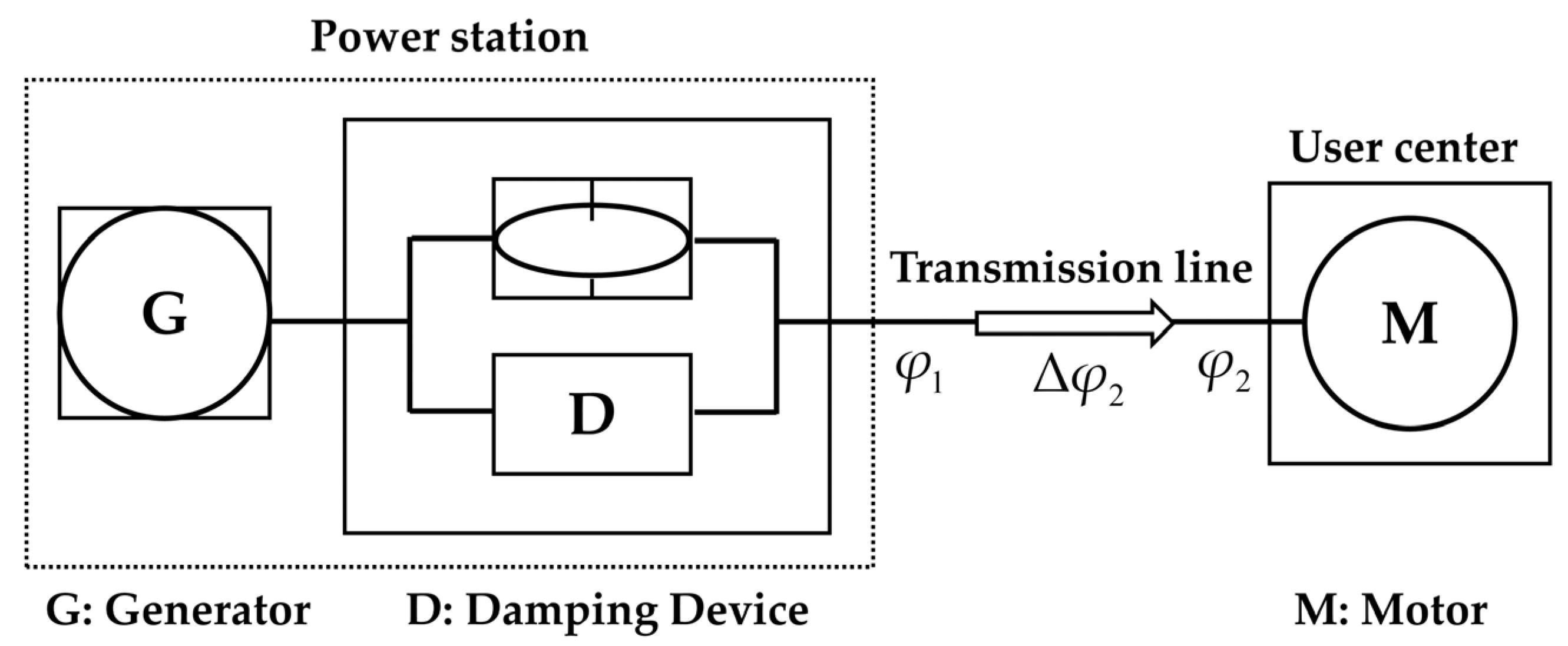
This section investigates wind turbine systems based on DFIGs, with their grid-connected model illustrated in Figure 3. Utilizing the mathematical model of DFIGs in the dq-axis synchronous rotating coordinate system [25], the active power output P_e of the DFIG can be calculated as follows:

$$P_e={\displaystyle \frac{3}{2}}{\omega }_r{L}_m(i_{rq}{i}_{sd}-i_{rd}{i}_{sq}),$$

(30)

where ${\omega }_r$ is the rotational angular velocity of the rotor; L_m is the equivalent mutual inductance between the stator and rotor windings in the dq-axis coordinate system; and i_rq, i_rd, i_sq, i_sd, represent the dq-axis current components of the stator and rotor.

By using stator vector control for rotor-side converter, the decoupling control of active and reactive output power of DFIG is realized, and then the stator and rotor currents are obtained as follows:

$$\left\{\begin{array}{l}{i}_{sd}={\displaystyle \frac{{\psi }_s-L_m{i}_{rd}}{L_s}}\\ i_{sq}={\displaystyle \frac{-L_m{i}_{rq}}{L_s}}\end{array}\right.,$$

(31)

where ${\psi }_s$ is the stator flux linkage; L_s is the self-inductance of stator winding in dq-axis coordinate system.

The active power output P_e of the DFIG is regulated by controlling the rotor q-axis current I_qr and the grid-side frequency ω_g. Substituting Equation (31) into Equation (30), the active power P_e of the DFIG is derived as expressed in Equation (32):

$$P_e={\displaystyle \frac{{\omega }_r{L}_m{I}_{qr}{U}_s}{L_s{\omega }_g}},$$

(32)

where U_s is the stator voltage.

For wind-integrated power systems employing the Maximum Power Point-Tracking (MPPT) control strategy, the output active power P_e matches the active power reference P$P_e^{ref}$. Consequently, the q-axis component of the rotor current I_qr aligns with its reference value $I_{qr}^{ref}$, as formulated in Equation (33):

$$I_{qr}=I_{qr}^{ref}={\displaystyle \frac{P_e^{ref}{L}_s{\omega }_s}{U_s{L}_m{\omega }_r}},$$

(33)

where ${\omega }_s$ is the natural frequency.

Based on Equations (32) and (33), the following relationships are derived:

$$P_e={\displaystyle \frac{P_e^{ref}{\omega }_s}{{\omega }_g}}.$$

(34)

When a system fault occurs, the frequency deviation relative to the nature frequency can be expressed by the following formula:

$${\omega }_g={\omega }_s+\Delta \omega ={\omega }_s+\dot{\theta },$$

(35)

where $\theta$ is the phase angle of the terminal voltage of the wind turbine generator, $\Delta \omega =d\theta /dt$.

Combining Equations (34) and (35), the active power output of the wind turbine generator is formulated as

$$P_e=P_e^{ref}-{\displaystyle \frac{P_e^{ref}}{{\omega }_s}}\dot{\theta }.$$

(36)

Wind turbine systems exchange electrical power with the grid via inverter interfaces, which inherently lack inertial characteristics. Consequently, a power system integrated with wind power can be represented by a hybrid first- and second-order Kuramoto-like model, as shown in the following formula:

$$\left\{\begin{array}{l}{M}_i{\ddot{\delta }}_i+D_i{\dot{\delta }}_i=P_i-{\displaystyle \sum _{j\in I_g}{P}_{max,ij}\sin ({\delta }_i-{\delta }_j)},i\in V_1\\ {\displaystyle \frac{P_{eh}^{ref}}{{\omega }_s}}{\dot{\theta }}_h=P_{eh}^{ref}-U_h^2{G}_{hh}-{\displaystyle \sum _{j=1}^n\left|U_h\right|\left|E_j\right|\left|Y_{hj}\right|\sin ({\theta }_h-{\theta }_j-{\phi }_{hj})},h\in V_2\end{array}\right..$$

(37)

4.3. Power System Transient Stability Criterion and Attraction Region Estimation

Based on the network model obtained in Section 4.1, the attraction region of transient stability equilibrium point is estimated by using the mathematical analysis method of non-uniform second-order Kuramoto model. Assuming a uniform damping-to-inertia ratio across all nodes in Equation (29), that is, D_i/M_i = α, the following simplified equation is obtained:

$${\ddot{\delta }}_i+\alpha {\dot{\delta }}_i={\displaystyle \frac{P_i}{M_i}}+{\displaystyle \frac{1}{M_i}}{\displaystyle \sum _{j\ne i}^N{P}_{ij}\sin ({\delta }_j-{\delta }_i)}.$$

(38)

Considering that when the system is running stably, ${\displaystyle {\sum }_{i=1}^N{P}_i}=0$, and the phase of each node changes with time t. The average phase ${\delta }_q$ is defined, and ${\delta }_q$ satisfies the following formula:

$$\left\{\begin{array}{l}{\ddot{\delta }}_q+\alpha {\dot{\delta }}_q=0\\ {\delta }_q={\displaystyle \frac{1}{N}}{\displaystyle \sum _{i=1}^N{M}_i{\delta }_i}\end{array}\right..$$

(39)

By solving the above formula, we can get

$${\delta }_q(t)={\delta }_q(0)+{\displaystyle \frac{1}{\alpha }}{\dot{\delta }}_q(0)(1-e^{-\alpha t}).$$

(40)

As the state quantity (δ₁(t), δ₂(t), …, δ_n(t)) of the generator power angle represents the spatial relative position between the rotors of each generator, and the difference in the maximum power angle of the generator reflects the transient stability of the power system, the O(δ) is defined to reflect the power angle characteristics, and the following formula is calculated:

$$O\left(\delta \right)=\max \left\{\Delta {\delta }_{\max },\Delta {\delta }_{\max }+{\displaystyle \frac{1}{\alpha }}\Delta {{\delta }^{\prime }}_{\max }\right\},$$

(41)

where Δδ_max is the maximum power angle difference between any two generators.

In addition, according to the maximum deviation of P_i/M_i reflecting the inherent force in the system that prevents the system from maintaining transient stability, the difference in the maximum power inertia ratio R(P) and the network topology parameter X reflecting the coupling strength of the system are defined as follows:

$$R(P)=\max \left\{{\displaystyle \frac{P_i}{M_i}}\right\}-\min \left\{{\displaystyle \frac{P_i}{M_i}}\right\},$$

(42)

$$X=\min \left\{\left({\displaystyle \frac{1}{M_i}}+{\displaystyle \frac{1}{M_j}}\right)P_{ij}+{\displaystyle \sum _{v\ne ij}\min \left\{\frac{P_{iv}}{M_i},\frac{P_{jv}}{M_j}\right\}}\right\}.$$

(43)

Among them, the values of O(δ) and R(P) change with time, and when the network structure of power system does not change, the value of network topology parameter X remains unchanged. By deduction, the differential inequality of Δδ_max is as follows:

$${\displaystyle \frac{d{\left(\Delta {\delta }_{\max }\right)}^2}{dt}}+{\displaystyle \frac{d\left(\Delta {\delta }_{\max }\right)}{dt}}\le R\left(P\right)-X\sin \Delta {\delta }_{\max }.$$

(44)

The condition of the above formula is X > 0, $\Delta {\delta }_{\max }\in \left(0,\pi \right)$. Based on the above formula, the properties of attraction region of power system network model are generalized: let X > R(P), and define $\gamma \in \left(0,\pi /2\right)$ as $\gamma =\arcsin \left(R(P)/X\right)$, assuming that

$$\gamma +{\displaystyle \frac{1}{\alpha }}\sqrt{2\left[\gamma R(P)-X(1-\cos \gamma )\right]}<\pi -\gamma ,$$

(45)

and the initial conditions of the system are satisfied $0<O\left({\delta }_0\right)<\pi -\gamma$, then $\Delta {\delta }_{\max }\le O\left({\delta }_0\right)$.

Based on the above formula, we can know that $\sqrt{2R(P)}/\alpha \times \sqrt{\gamma -\tan \gamma /2}/\left(\pi -2\gamma \right)=1$ has a unique solution γ_s in $\gamma \in \left(0,\pi /2\right)$ through the monotonicity analysis of the function, so the prerequisite of the nature of this attraction region can be written as $X>{R(P)/\sin \gamma }_s$.

Based on the above, the parameter definitions and stability criteria used to determine the transient stability state of the system after disturbance are proposed as follows:

$$\left\{\begin{array}{l}a:O\left(\delta \right)=\max \left\{\Delta {\delta }_{\max },\Delta {\delta }_{\max }+{\displaystyle \frac{1}{\alpha }}\Delta {{\delta }^{\prime }}_{\max }\right\}\\ b:R(P)=\max \left\{{\displaystyle \frac{P_i}{M_i}}\right\}-\min \left\{{\displaystyle \frac{P_i}{M_i}}\right\}\\ c:{\displaystyle \frac{\sqrt{2R(P)}}{\alpha }}{\displaystyle \frac{\sqrt{\gamma -\tan \gamma /2}}{\pi -2{\gamma }_s}}=1\\ d:X>{\displaystyle \frac{R(P)}{\sin {\gamma }_s}}\\ e:\gamma =\arcsin \left({\displaystyle \frac{R(P)}{X}}\right),\gamma \in \left(0,{\gamma }_s\right)\\ f:0<O\left(\delta \right)<\pi -\gamma \end{array}\right..$$

(46)

When the system parameters meet the criteria c and d, according to the definition of γ in e, if the disturbance elimination moment O(δ) meets the criterion f, the system can restore transient stability after being disturbed, otherwise it will be unstable. If the precondition is not met, the criterion becomes invalid.

The network topology parameter X reflects the strength of network coupling connection, and the larger X is, the stronger the system’s ability to resist transient instability; R(P) represents the inherent ability to interfere with the transient stability of each generator, and the smaller R(P) is, the stronger the system’s transient stability is. The criterion requires that X > R(P)/sinγ_s is conservative, and the smaller γ_s is, the more conservative it is.

In order to study the limit time t_n of fault removal, the transient stability of the system after fault removal is judged according to whether the system state variable O(δ) is in the attractive region $\pi -\gamma$ at the time of fault removal: if O(δ) is in this region, the system can maintain transient stability; otherwise, it will experience transient instability.

5. Case Study

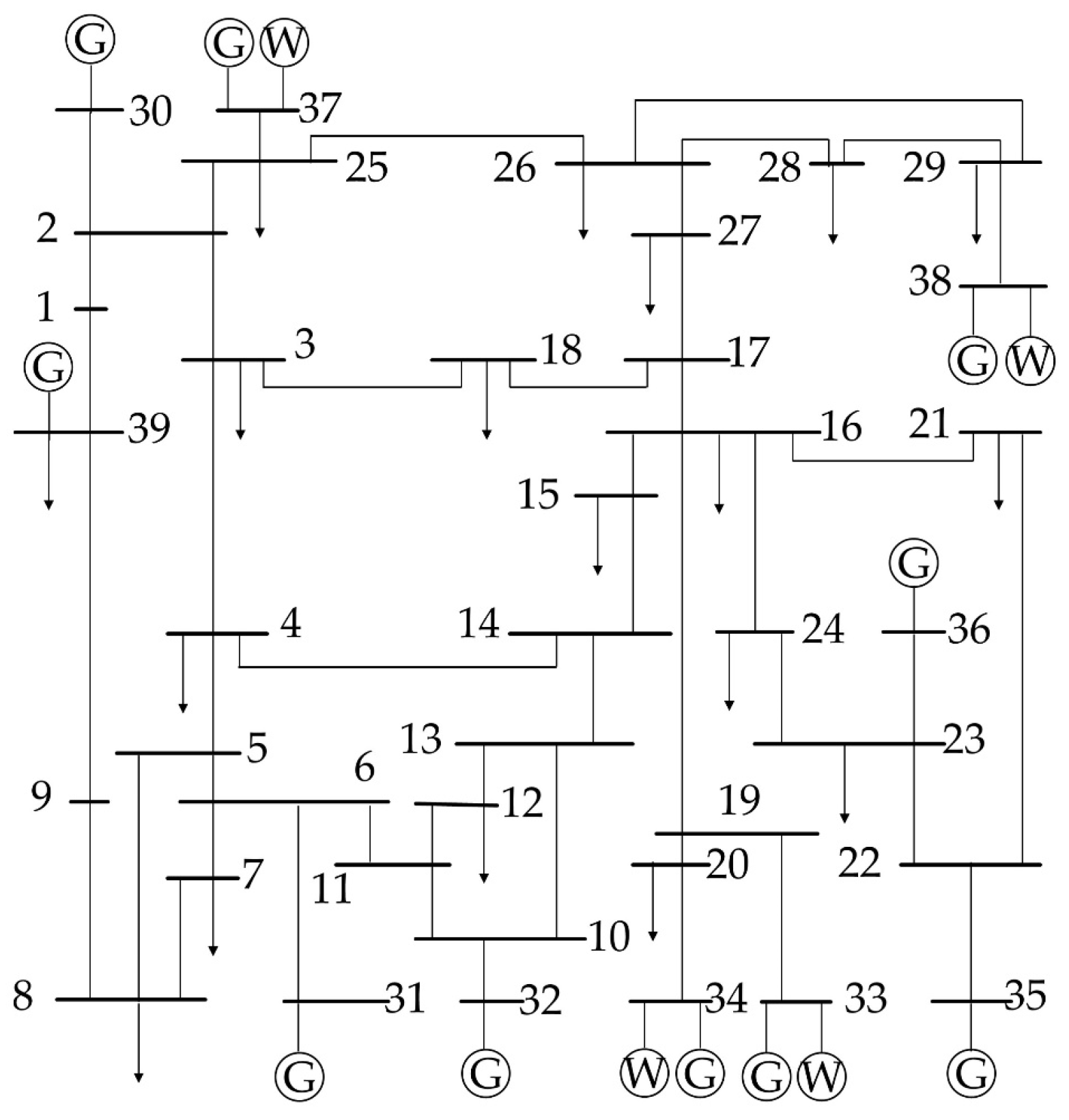
This paper verifies the effectiveness of the proposed model and algorithm by improving the IEEE 39-bus test system, and the system structure diagram is shown in Figure 4. The capacities of the wind turbines at nodes 33, 34, 37, and 38 are 500 MW, 350 MW, 450 MW, and 300 MW, respectively. At this point, the installed wind power capacity accounts for 20% of the total capacity.

5.1. Critical Node Identification

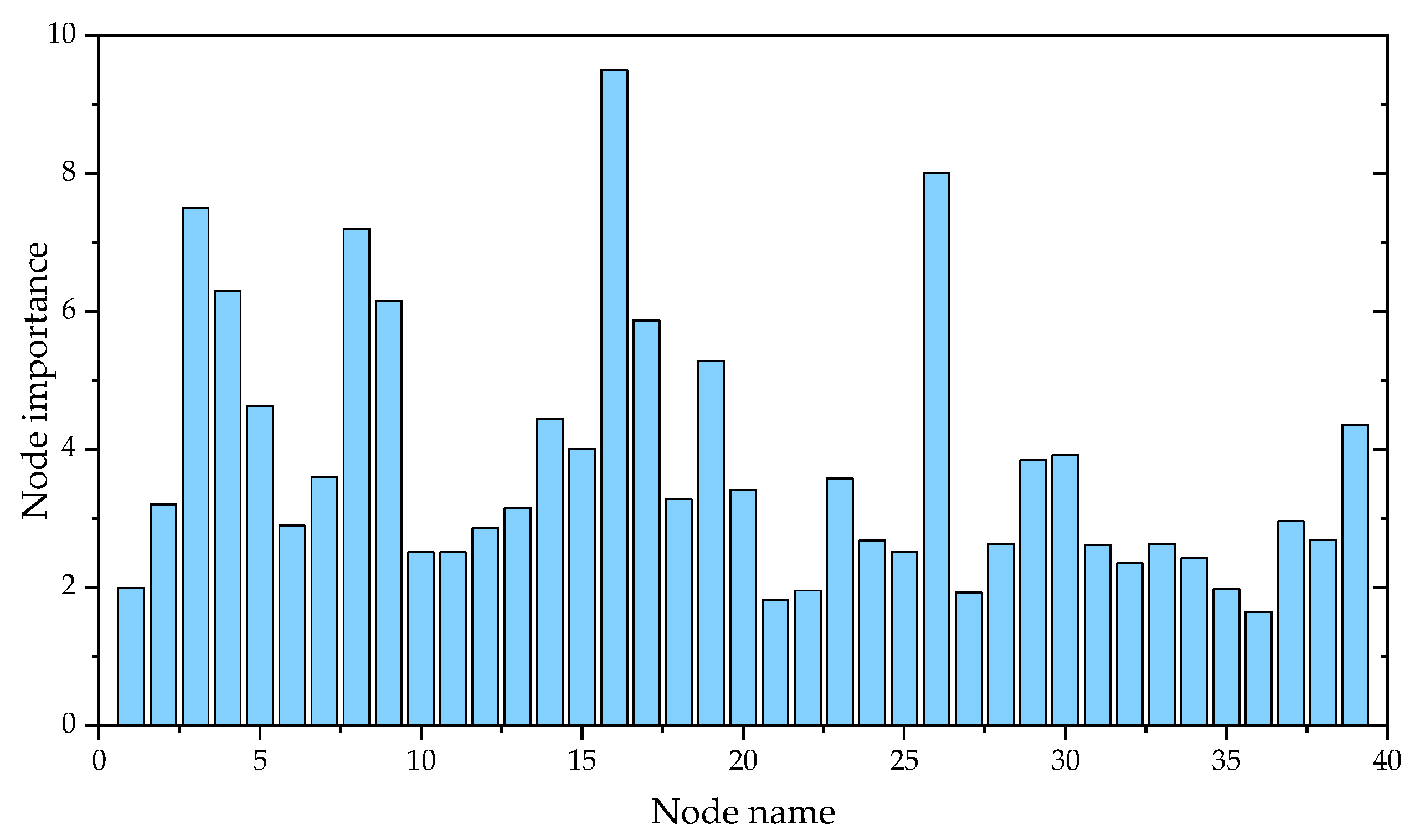
Comprehensively improve the iterative results of the PageRank algorithm and the voltage influence index to assess the importance of system nodes, as illustrated in Figure 5.

Node 16 is connected to five transmission lines and simultaneously handles the power output from six generators. The line 16–19 is the only path for the power output from generators 33 and 34. If node 16 is disconnected, the power grid will be separated into three parts. The islanding power balance and the flow transfer process will cause difficulties in power delivery from the generators and lead to significant load losses. Therefore, when considering the transmission efficiency of the power system for node importance ranking, node 16 ranks the highest. Nodes 26, 3, and 8 are important hubs for power exchange in the system, responsible for power aggregation and distribution, and are also significant load nodes. Additionally, removing nodes 4, 9, 17, 19, 5, and 14 may impact the power delivery from some generators, leading to power imbalance in the system. These nodes also have higher importance. Moreover, node 39, which is both a generator and a load node, has the highest generator output and load size. Therefore, in the process of quantifying node transmission efficiency, node 39 is considered more important than other generator nodes.

To further verify the effectiveness of the proposed node importance ranking method, a comparison is made with the top 10 nodes in the studies of reference [26], which considers load supply identification, and reference [27], which uses graph theory-based identification methods. The results are shown in

Table 1. Comparison results of node importance of improved IEEE 39-bus system.

Rank	The Method in This Paper	The Method in Reference [26]	The Method in Reference [27]
1	16	39	16
2	26	6	17
3	3	16	3
4	8	38	4
5	4	29	14
6	9	8	18
7	17	20	15
8	19	4	5
9	5	10	6
10	14	22	24

.

5.2. Influence of Coupling Mode on Synchronization Performance of Power System

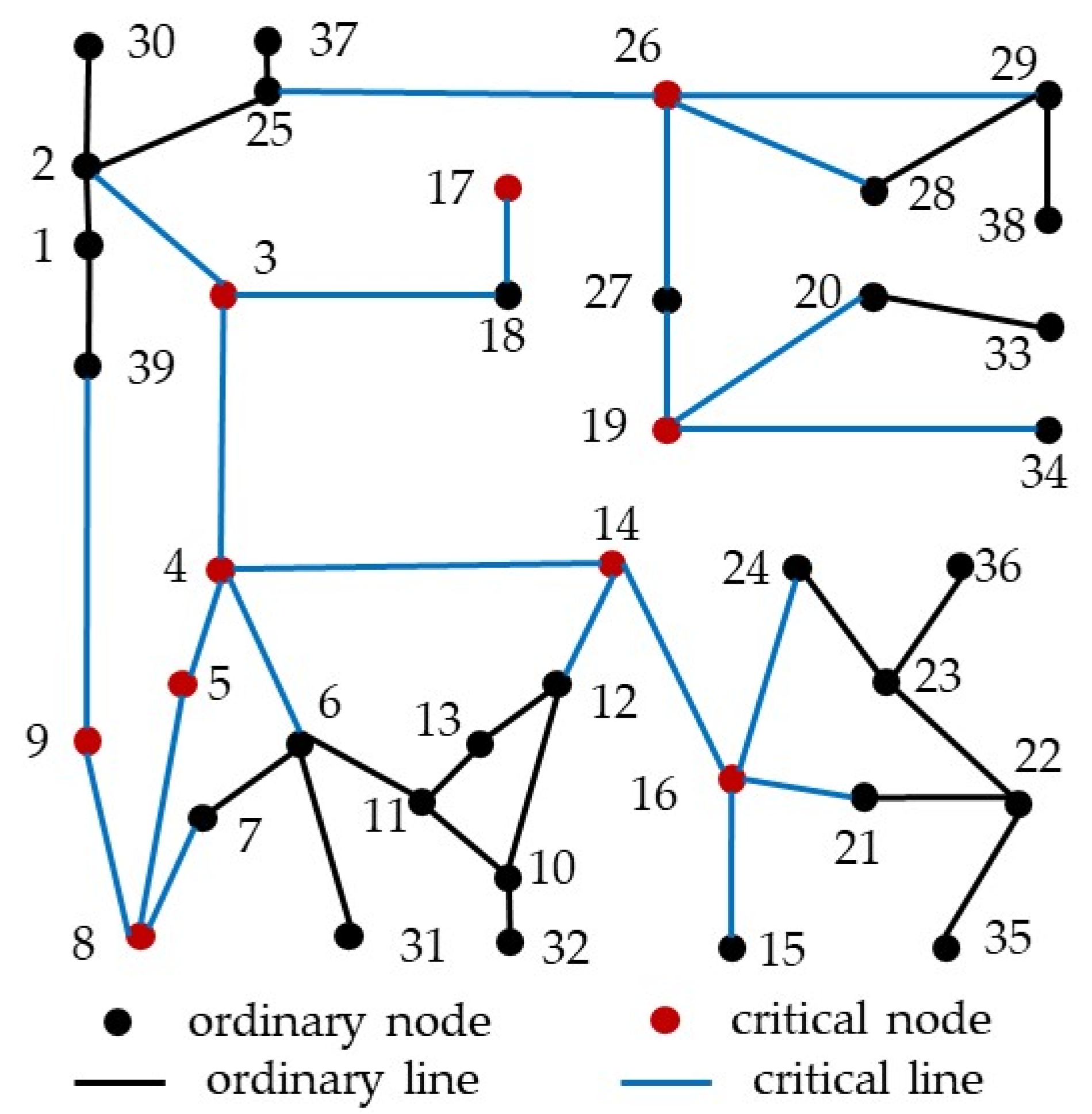
To verify the impact of node importance on the synchronization performance of the power system, the IEEE 39-bus network model constructed in the previous section is used, and a simulation analysis is conducted. The topology of the system is shown in Figure 6, where the red nodes represent the critical nodes of the system, and the blue lines highlight the edges connecting the critical nodes to their direct neighboring nodes, with a total of 23 edges. Additionally, to quantitatively analyze the synchronization level of the system, the following order parameter is defined:

$$r(t)e^{j\psi (t)}={\displaystyle \frac{1}{N}}{\displaystyle \sum _{i=1}^N{e}^{j{\theta }_i(t)}},$$

(47)

where $\psi (t)$ is the average value of the phases of all phase oscillators in the system.

After the power system reaches a steady state, the average order parameter can be defined as the average value of the ordered parameter modulus in a period of time under a steady operation state, as shown in the following formula:

$$r=\underset{t_1\to \infty }{\lim }{\displaystyle \frac{1}{t_2}}{\displaystyle {\int }_{t_1}^{t_1-t_2}\left|r(t)\right|dt},$$

(48)

where t₁ is the time when the system enters the synchronous state; t₂ is a time after the system is in synchronous operation.

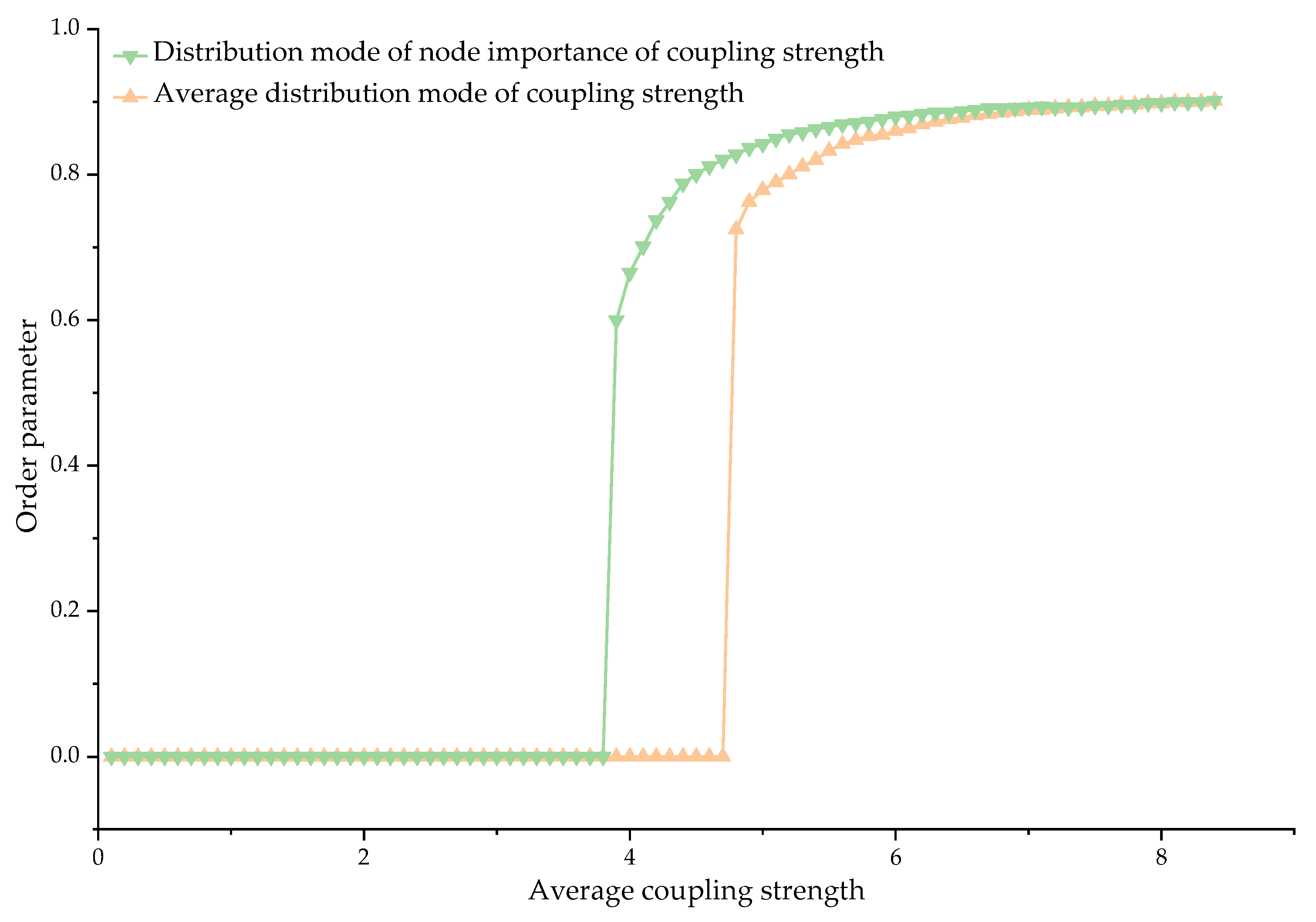
The coupling strength is distributed according to node importance, with the coupling strength between the system’s critical nodes and their neighboring nodes being increased, while the coupling strength of other lines is correspondingly decreased. This results in the coupling strength of the lines shown in blue in the diagram accounting for 70% of the total coupling strength. Two approaches are used for this distribution: one with a uniform distribution of coupling strength and the other with coupling strength distributed according to node importance. By continuously increasing the system’s average coupling strength, the relationship between the order parameter r and the system’s average coupling strength is observed, as shown in Figure 7.

By comparing the synchronization performance differences in the system under the two coupling methods shown in Figure 7, it can be concluded that the average critical coupling strength of the system is smaller and the synchronization performance of the system is better than that of the uniform distribution of coupling strength and the distribution of coupling strength according to the importance of nodes. In the Kuramoto-like model of power system, the coupling strength between nodes is directly proportional to the transmission line capacity. Therefore, this conclusion can guide the distribution of transmission line capacity to improve the performance of power system.

5.3. Transient Performance Analysis of Power System After Fault

For the improved IEEE 39-bus system, three fault scenarios are set up and the fault limit removal time is calculated. The results are compared and analyzed to verify the rationality of this method. Let the initial fault removal time t₁ = h = 0.0 ls, in which the fault scenario 1 is a three-phase short circuit in the node 7 of test system. By using the calculation method of fault limit removal time in this paper, the limit removal time of scenario 1 is obtained. Relevant parameters and resection time are shown in

Table 2. Scenario 1 Estimation parameters of fault limit removal time.

Parameter	X	R(P)	γ	$\mathit{\pi }-\mathit{\gamma }$	γs	tn	O(δ)
Value	62.522	18.732	0.304	2.838	1.243	1.09 s 1.10 s	2.835 2.842

.

Fault Scenario 2 involves a three-phase short circuit fault occurring at node 26 in the test system and uses the method described in this paper to calculate the fault limit removal time of scenario 2.

Table 3. Scenario 2 estimation parameters of fault limit removal time.

Parameter	X	R(P)	γ	$\mathit{\pi }-\mathit{\gamma }$	γs	tn	O(δ)
Value	62.522	30.203	0.502	2.640	1.152	0.65 s 0.66 s	2.632 2.645

shows the estimation results of corresponding system parameters and resection time.

Fault Scenario 3 involves a three-phase short circuit fault occurring at node 21 in the test system. After solving for the critical fault clearing time, the results are presented in

Table 4. Scenario 3 Estimation parameters of fault limit removal time.

Parameter	X	R(P)	γ	$\mathit{\pi }-\mathit{\gamma }$	γs	tn	O(δ)
Value	62.522	25.622	0.421	2.721	1.195	0.89 s 0.90 s	2.716 2.730

.

At the same time, the standard test system is simulated in time domain, and the fault removal time is constantly modified under the above three fault scenarios, and the fault removal time is selected with the same step size h = 0.01s as above, and the time domain simulation results of the maximum power angle difference in the generator are observed. If the maximum power angle difference in the system generator is less than or equal to 180°, the system is considered to be transient stable; If the maximum power angle difference in the system generator is greater than 180°, the system is transient unstable, so as to determine the fault limit removal time under the time domain simulation calculation. The comparison between the method in this paper and the time domain simulation results is shown in

Table 5. Comparison of the results of fault limit removal time between this method and time domain simulation.

Fault Scenario	The Method in This Paper	Time Domain Simulation Results	Efficiency
Scenario 1	1.09 s	1.17 s	6.84%
Scenario 2	0.65 s	0.75 s	13.33%
Scenario 3	0.89 s	0.98 s	9.18%

.

The fault limit removal time is used to reflect the transient stability of power system. The shorter the limit removal time, the worse the system stability will be, and it shows that the system is more prone to transient instability. Comparing the estimation method of fault limit removal time proposed in this paper with the time domain simulation results, it is found that the relative error of the two methods is small, thus verifying the rationality of this method. At the same time, the fault limit removal time obtained by this method is short, which shows that the stability margin of the actual system is larger than the estimated result, so this method is conservative and can ensure the safe and stable operation of the system. By comparing the results in Table 2, Table 3, Table 4 and Table 5, it can be found that the closer the γ_s is to π/2, the smaller the relative error of the estimation result of fault limit removal time, and the parameters reflect the conservatism of this method, which is consistent with the parameter analysis result of transient stability criterion in Section 4.3. The analysis error is mainly caused by the introduction of a large number of inequalities in the mathematical derivation of the range estimation of the attraction region of the equilibrium point. Due to the gradual amplification of the inequalities, the derived transient stability criterion is conservative, resulting in a small estimation result of the fault limit removal time.

6. Conclusions

This study addresses the transient stability challenges in wind-integrated power systems through a novel node importance-based Kuramoto-like model. The key contributions include the following:

(1)

Critical node identification: An improved PageRank algorithm incorporates electrical metrics (transmission efficiency, voltage influence) and virtual nodes to quantify node importance. Critical nodes are identified as hubs for suppressing fault propagation and maintaining grid coherence.

(2)

Hybrid oscillator model: A hybrid Kuramoto-like model integrates second-order synchronous generators and first-order wind turbines. By dynamically redistributing coupling strengths based on node importance, local synchronization robustness is enhanced, reducing the system’s vulnerability to disturbances.

(3)

Stability criterion and validation: Using attraction region theory, stability criteria are derived by balancing network topology parameters X and maximum power inertia ratio R(P). The proposed method estimates fault limit removal time with conservative margins, validated by time-domain simulations showing less than 10% error.

Compared with the existing methods, the advantages of the framework proposed in this paper are shown in

Table 6. Comparison of advantages between this method and other methods.

Comparison Dimension	The Method in This Paper	Traditional Time Domain Simulation	Extended Equal Area Criterion	Pure Kuramoto Model (Uniform Coupling)
Core Advantages	Non-uniform coupling, hybrid modeling	Accurate nonlinear component modeling	Rapid analytical assessment suitable for online applications	Simple model with high computational efficiency
Input Data	Grid topology parameters, node importance metric, wind turbine dynamic parameters	Detailed parameters for all components	Synchronous machines inertia, damping, and electromagnetic power parameters	Topology connections, uniform coupling strength
Computational Efficiency	Medium: Kron reduction reduces the dimension	Low: High computational load for complex systems	High: Rapid analytical derivation, limited by multiple equilibria	High: Simple first-order model but with dynamic characteristic distortion
Topology Change Adaptability	Strong: Coupling strength reallocation for topology changes	Medium: Requires full-system remodeling	Medium: Equilibrium point calculation affected by topology	Weak: Uniform coupling ignores topological heterogeneity

:

The proposed methodology offers a foundational tool for designing resilient power grids in the era of renewable energy dominance. Future work might extend this approach to multi-energy systems and incorporate real-time data-driven adjustments for adaptive stability control. It should be noted that the proposed model is currently optimized for transient stability analysis under synchronous frequency conditions. While its node importance-based coupling mechanism and hybrid-order modeling provide a theoretical foundation for topological analysis, explicit consideration of sub-synchronous frequency components, shaft torsional dynamics, and stochastic process modeling is required to enable applications in sub-synchronous oscillation studies.