Abstract
Load forecasting plays a crucial role in power system planning and operational dispatch management. Accurate load prediction is essential for enhancing power system reliability and facilitating the local integration of renewable energy. This paper proposes a hybrid approach combining traditional time series models (ARIMA) with machine learning models (SVR). The particle swarm optimization (PSO) algorithm is improved by adjusting its elastic momentum, and the enhanced APSO algorithm is employed to optimize the adaptive weights of the hybrid model. Consequently, an elastic momentum-enhanced adaptive weighted load forecasting model (APSO-ARIMA-SVR) is developed. Numerical simulations using real-world datasets validate the model’s effectiveness. Results demonstrate that the proposed APSO-ARIMA-SVR model achieves optimal fitting performance, with prediction errors of 274.23 (MAE) and 321.50 (RMSE), representing the lowest errors among all comparative models.
1. Introduction
The primary objectives of power load forecasting are to enhance electricity utilization efficiency, balance power supply and demand, and provide accurate information support for formulating electricity trading strategies and dispatch planning. Particularly in modern power systems with high penetration of renewable energy, the accuracy of load forecasting significantly impacts grid planning, electricity trading, system maintenance, and energy dispatch. Both economic operations and dispatch management heavily rely on precise load forecasting. As a critical determinant of power system reliability and cost-effectiveness, load forecasting has become a pivotal concern for power system operators and researchers [1]. Therefore, improving the accuracy of power load forecasting holds substantial significance for power systems.
Load forecasting can be categorized into four types based on temporal resolution: ultra-short-term, short-term, medium-term, and long-term forecasting [2]. Long-term and medium-term forecasts are critical for strategic planning in power system development, while the accuracy of short-term load forecasting directly impacts generation scheduling, power system dispatch, economic operations, and electricity markets [3]. The primary distinction between long-term and short-term forecasting models lies in their input variables. Long-term forecasting typically employs historical annual consumption data as primary inputs [4], supplemented by macroeconomic indicators such as Gross Domestic Product (GDP), per capita GDP, and population demographics [5]. In contrast, short-term and ultra-short-term forecasting models integrate weather conditions, seasonal patterns, and real-time operational data alongside historical load profiles [6]. The growing penetration of renewable energy has elevated the importance of short-term forecasting for mitigating operational risks, reducing management costs, and enhancing reliability in modern power systems [7]. Given its pivotal role in ensuring economic viability, operational security, and electricity market efficiency, short-term load forecasting has emerged as a primary research focus for global scholars in recent years.
Currently, commonly used forecasting models mainly include statistical methods [8], time series forecasting models [9], and soft computing techniques [10,11]. Statistical models encompass multiple regression [12,13] and autoregressive (AR) models [14]. The most commonly used time series models primarily include the autoregressive integrated moving average (ARIMA) framework [15,16] and grey system methods (GMs) [17]. ARIMA is a renowned time series forecasting method proposed by Box and Jenkins [18] in the early 1970s. Its fundamental principle involves transforming a non-stationary time series into a stationary one, and then regressing the dependent variable solely on its lagged values, as well as the current and lagged values of the random error term. ARIMA is very suitable for capturing the correlation between short-term data. The model principle is relatively simple and has a wide range of applications in energy forecasting [19,20,21]. GMs, proposed by Chinese scholar Professor Deng Julong in 1982 [22], focuses on the analysis, modeling, prediction, decision-making, and control of systems with incomplete information. The grey prediction model (GM), as a core component of this theory, demonstrates strong performance in time series forecasting with limited data samples [23,24,25].
In recent years, with the advancement of artificial intelligence (AI) research, soft computing techniques such as neural networks and machine learning based on AI have gradually been introduced into the field of energy management [26,27]. Compared with conventional statistical methods and time series forecasting approaches, soft computing techniques demonstrate superior capability in handling complex nonlinear variations while achieving enhanced fitting accuracy [28,29]. AI models such as artificial neural networks (ANNs) [30,31], support vector machines (SVMs) [32,33], federated learning (FL) [34,35,36], and deep learning (DL) methods [37,38,39] have gained prominence, with ANNs being widely adopted due to their universal approximation capability when configured with sufficient hidden layers and nodes. However, ANNs suffer from challenges including parameter initialization sensitivity, slow convergence, undesirable local minima, and scalability limitations [40]. SVM represent a robust methodology that effectively balances model learning capacity and complexity under limited sample sizes while demonstrating strong generalization performance. Characterized by their small-sample training requirements and high interpretability, SVMs have been extensively applied in the domain of electric load forecasting [41]. DL architectures like deep belief networks (DBNs) [42,43] and recurrent neural networks (RNNs) [44,45], Long Short-Term Memory (LSTM) [46,47] and Transformer [48,49,50], while widely adopted in predictive research, require substantial training samples and may suffer from overfitting issues [51]. Singh et al. [52] proposed a novel hybrid model that integrates wavelet transform with SVM to construct an electric load forecasting framework. This approach calculates and further decomposes the error terms of sub-sequences within the combined model, thereby enhancing its overall predictive capability. Zeng [53] questioned the performance of Transformer in long-term series prediction and introduced a set of single-layer linear models, LTSF Linear, to compare with Transformer. It was found that the performance was better than that of complex LTSF models based on Transformer. We have summarized several commonly used prediction models, as shown in Table 1.

Table 1.
Summary of several models commonly used for prediction.
Compared to single-model approaches in load forecasting, hybrid models integrate the strengths of individual predictors to achieve superior prediction accuracy [54], typically combining two or more methodologies where each component enhances precision and operational effectiveness [55]. The selection of individual methods within a composite model must be determined by the characteristics of the data type, the applicable scope of the models, and the prediction objectives [56]. Among the challenges in model construction, one of the most critical is the appropriate determination of weighting schemes. Currently, widely adopted weighting methodologies include inverse variance weighting [57], standard deviation-based allocation [58], entropy-based weighting [59], and optimization-driven approaches [60]. Yang et al. [61] proposed an ensemble model integrating Rank-based Set Pair Analysis (R-SPA), radial basis function (RBF) networks, and AR components to enhance precipitation forecasting accuracy, with optimal weight allocation achieved through genetic algorithm optimization. Wang et al. [62] developed a multivariate ensemble model and employed an improved multi-objective coati optimization algorithm (IMOCOA) to determine optimal weight coefficients for constituent models, thereby enhancing the hybrid model’s predictive performance. Wang et al. [63] proposed a hybrid PSO-SVM-ARMA forecasting model for wind power prediction, ARMA with PSO-SVM. The optimal weight coefficients were determined through covariance minimization and PSO algorithms to enhance prediction accuracy and stability.
Therefore, based on analyzing the characteristics and application scopes of commonly used time series prediction models and support vector machines, this paper addresses the short-term power load forecasting problem by constructing a hybrid prediction model using the Rolling Grey Model (RGM), ARIMA, and Support Vector Regression (SVR). Additionally, elastic momentum is introduced to optimize the inertia weight in the particle swarm optimization (PSO) algorithm, proposing an improved PSO referred to as APSO. The APSO is then employed to optimize the weights of the hybrid prediction model, thereby establishing an adaptive hybrid forecasting model with high accuracy and strong generalization capability, named APSO-ARIMA-SVR. Subsequently, the proposed hybrid forecasting model was benchmarked against three established methods—ARIMA, RGM, and SVR—through practical case studies to validate its effectiveness. More specifically, the contributions of our work are as follows:
- (1)
- We propose an adaptive inertia weight adjustment method for PSO. Since inertia weight is the predominant factor governing the search capability of particle swarm in PSO, we develop an adaptive inertia weight adjustment mechanism to enhance the algorithm’s self-adaptation in optimization processes. Comprehensive comparative experiments conducted on benchmark functions validate the effectiveness of the proposed improvement method.
- (2)
- We conducted a comparative analysis of commonly used single prediction models, examining the characteristics and applicable scenarios of different model types. Through case studies, we validated the prediction performance and identified an optimal short-term load forecasting model with superior accuracy and efficiency.
- (3)
- We propose a hybrid forecasting model with adaptive momentum based on an improved PSO. By employing an enhanced particle swarm optimization approach with adaptive inertia weights, the model dynamically determines the optimal combination weights for two forecasting sub-models. This architecture enables autonomous weight adjustment based on individual model predictions and target objectives, thereby significantly improving load forecasting accuracy.
The remainder of this paper is structured as follows: Section 2 introduces the fundamental methodologies of RGM, ARIMA, and SVR. Section 3 details the construction of the hybrid forecasting model. In Section 4, a case study is presented, followed by model simulation and comprehensive feasibility analysis based on the simulation results. Finally, Section 5 concludes the paper and outlines potential future research directions.
In future research, we will conduct comparative experiments with state-of-the-art models from the literature while continuously refining and enhancing the proposed forecasting framework.
2. Model Framework and Theoretical Principles
2.1. Model Framework
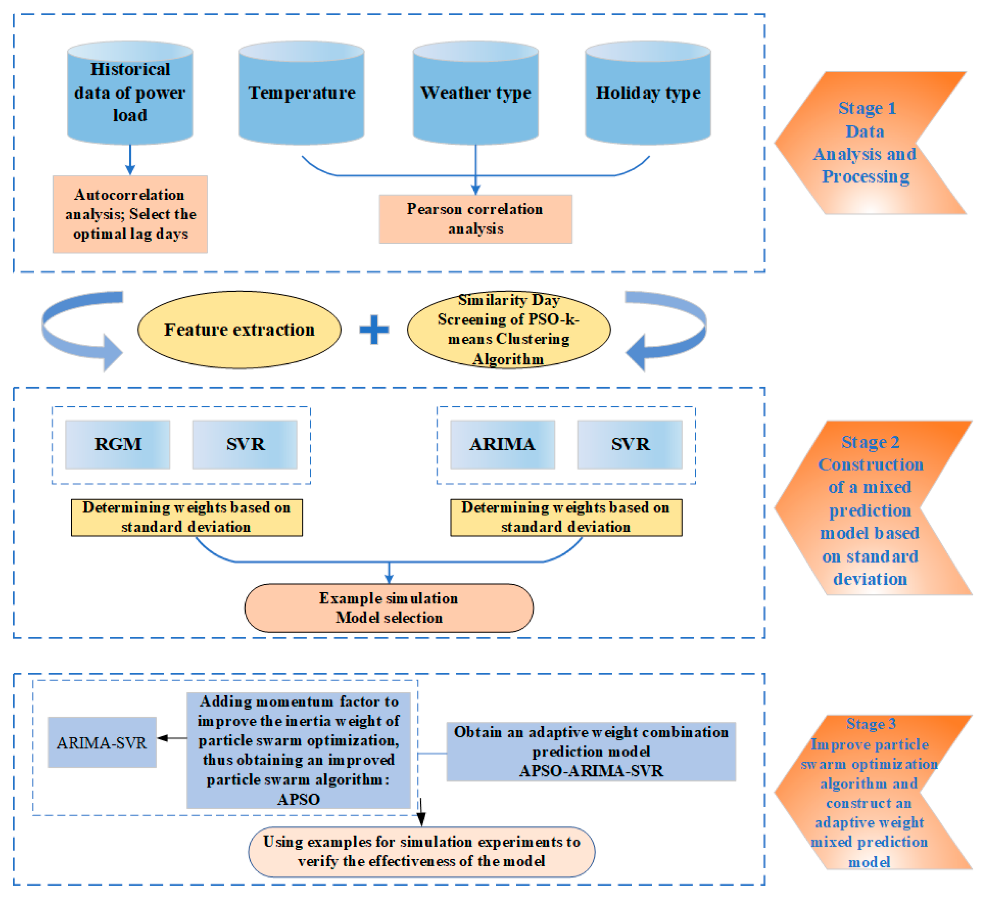
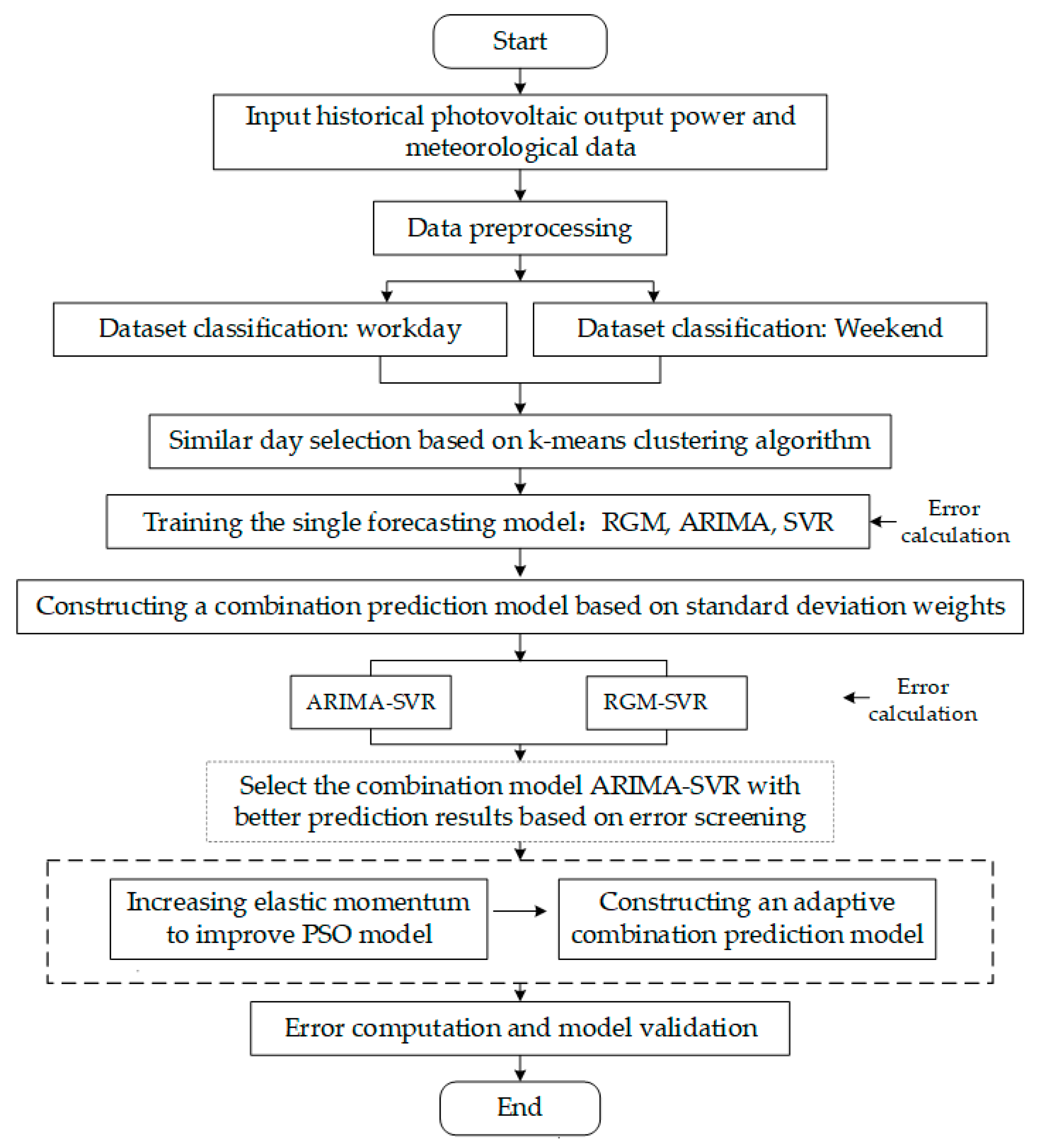
This study organically integrates grey prediction models, regression models, and machine learning models to construct a hybrid forecasting framework for power load prediction. Notably, an innovative adaptive weighting mechanism is introduced by incorporating elastic momentum into the PSO to optimize the weight allocation within the hybrid forecasting framework. The improved PSO synergistically combines GMs and machine learning models, establishing an adaptive weighted hybrid forecasting model to enhance prediction accuracy. The detailed modeling architecture is illustrated in Figure 1.
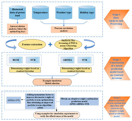
Figure 1.
Modeling framework.
Stage 1: Data Collection and Preprocessing
Multi-source datasets are collected, cleaned, and preprocessed. Autocorrelation analysis is applied to historical power load data to determine optimal lag days, while Pearson correlation analysis identifies critical meteorological features from weather data.
Stage 2: Standard Deviation-based Hybrid Forecasting Model
A dual-model hybrid framework is constructed by strategically combining ARIMA and RGM with SVR. Model weights are dynamically calculated through standard deviation analysis of prediction residuals, establishing a deviation-optimized hybrid forecasting architecture tailored for ultra-short-term load characteristics.
Stage 3: Adaptive Hybrid Model with Enhanced PSO
The PSO is enhanced with elastic momentum mechanisms to overcome local optima limitations. The improved Adaptive PSO (APSO) algorithm optimizes weight allocation in the hybrid model, forming an adaptive hybrid forecasting framework (APSO-ARIMA-RGM-SVR) with validated high accuracy and enhanced generalization capability across diverse operational scenarios.
2.2. Single Prediction Model
2.2.1. Rolling Grey Model
The simplest GM (1,1) model requires only four historical data points for training to generate predictions, making it particularly advantageous in forecasting domains where industrial datasets often suffer from limited sample sizes. This model enables reliable predictions in small-sample scenarios or fields with partial data missing. The construction of the GM (1,1) model involves three key steps: the Accumulated Generating Operation (AGO), the Inverse Accumulated Generating Operation (IAGO), and the establishment of the GM (1,1) prediction model. The detailed modeling procedure is as follows [64]:
Step 1:
Set a as the original sequence,
where perform the first-order Accumulated Generating Operation (1-AGO) on the original sequence to obtain the generated sequence,
Step 2:
Assume the sequence is continuously differentiable and satisfies the following first-order linear differential equation,
where Parameters a, u are undetermined coefficients to be solved.
Step 3: Discretize Equation (3) to transform the differential equation into the following difference equation:
where , is a background value sequence constructed by ,
generally, is set to 0.5.
Step 4: Solve for parameters a and u:
By applying the least squares method, we can solve for parameters a and u in Equation (3).
Step 5: The prediction formula is established as follows:
With parameters a and u obtained, solving Equation (7) yields:
A cumulative deduction is generated on the above formula, and the prediction formula is obtained:
In theory, as the prediction interval increases, future uncertainties may exert certain influences on the forecasting system. For the GM (1,1) prediction model, the initial few data points following are relatively accurate and less affected by uncertain factors. However, as the prediction timeline extends further, the forecasted data can only serve as planning-oriented reference values.
Accordingly, an enhanced forecasting methodology is proposed: Initially, a GM (1,1) model is constructed based on the known data sequence to predict a grey value, which is subsequently incorporated into the original sequence to form an updated information set. With each newly added data point, an updated GM (1,1) model is established. To address the diminishing representational capacity of historical data in reflecting emerging trends, an iterative replacement mechanism is implemented to maintain a fixed sequence length while refreshing the dataset. Through this rolling update approach, model parameters undergo continuous refinement at each prediction step, thereby achieving progressive model improvement. The resultant predictions are generated dynamically within this adaptive framework. This advanced methodology is formally designated as the “Grey Prediction Model with Rolling Mechanism (RGM)”. The specific modeling procedure is as follows:
Step 1: The GM (1,1) model is established based on the original dataset.
Step 2: Prediction results in a new predicted value, denoted as , which is added to the original data while the oldest original data point is removed to maintain the constant dimension of the original data. The newly formed sequence is recorded as .
The GM (1,1) model is established by .
Step 4: The next value is predicted and recorded as . It is then appended to , and the oldest datum is discarded to generate the new sequence .
2.2.2. ARIMA
Non-stationary time series exhibit strong stochastic characteristics. In 1970, Box and Jenkins proposed a stochastic theory-based time series analysis approach, which effectively addresses forecasting challenges for non-stationary series [65]. The fundamental models include: Autoregressive (AR) models, Moving Average (MA) models, and ARIMA models. The ARIMA model specifically employs AR components, Integration terms, and MA components to analyze and model the disturbance terms in the series. This modeling methodology utilizes an extrapolation mechanism to characterize temporal patterns, while incorporating historical values, current values, and error terms of the predictive variables, thereby significantly enhancing forecasting accuracy.
For an integrated series Yt, stationarity is achieved via d-th order differencing, producing a stationary series Xt that admits an ARMA (p, q) representation.
where represents the model parameter, cc is a constant term, and ut denotes a white noise sequence.
The MA (q) model, denoting a moving average model of order q, can be expressed as:
where is the model parameter, denotes the expected value of Xt (typically assumed to be zero), and represents the error term of the white noise sequence.
The ARMA (p, q) model is formally expressed as:
The ARIMA (p, d, q) model is derived by applying d-th order differencing to an process, formally expressed as:
The ARMA (p, q) model extends to an ARIMA (p, d, q) model after applying d-th order differencing. In the ARIMA (p, d, q) specification: p denotes the order of the autoregressive component AR (p); d represents the degree of differencing; q indicates the order of the moving-average component MA (q).
The establishment of an ARIMA (p, d, q) model and its parameter determination can be summarized into four key steps:
(i) First, the stationarity of the time series must be verified, as a stationary time series represents the fundamental requirement for model construction. For non-stationary series, appropriate differencing transformations should be performed.
(ii) Subsequently, the model parameters need to be determined. The differencing order d can be identified through unit root tests, while the optimal autoregressive order p and moving average order q can be determined by examining the autocorrelation function (ACF) and partial autocorrelation function (PACF).
(iii) Following parameter specification, diagnostic checking should be conducted to verify the statistical significance of all estimated parameters and ensure the model’s adequacy through residual analysis.
(iv) Finally, the model should be validated through in-sample fitting to confirm the appropriateness of the selected ARIMA (p, d, q) specification.
2.2.3. SVR
SVM was first proposed by Vapnik and Cortes in 1995 [66]. SVM is designed to analyze the information contained in limited sample data while reducing model complexity and enhancing learning capability, thereby optimizing predictive performance. Moreover, SVM is not affected by challenges such as high dimensionality or overfitting, demonstrating superior generalization ability in addressing small-sample, high-dimensional, and nonlinear problems.
SVR is an extension of SVM for regression analysis, which introduces an -insensitive loss function to adapt classification methods for predictive regression tasks. Similarly to SVM in classification, SVR seeks an optimal regression hyperplane in the feature space that minimizes the total deviation of all training data points from this hyperplane.
The fundamental principle of SVR involves mapping input variables x into a high-dimensional feature space via a nonlinear transformation , where linear regression is performed to derive the target function f (x). The modeling procedure consists of the following steps:
Step 1: Given a dataset , where xi represents the input features, yi denotes the corresponding target values, and n indicates the total number of data points, the regression function to be determined is expressed as follows:
where and b are the parameters to be identified.
The parameters and b are estimated based on the structural risk minimization principle.
where is the confidence risk, C the penalty parameter, the insensitivity coefficient (for fitting accuracy control), with and being slack variables.
Step 3: To facilitate the solution, Equation (14) is transformed into its dual problem, yielding the nonlinear function:
where and are support vector parameters, and denotes the kernel function.
Step 4: According to Mercer’s condition, the kernel function is defined. Since the radial basis function (RBF) serves as a versatile kernel capable of achieving nonlinear projection, the RBF kernel is selected as follows:
The substitution of Equation (16) into Equation (15), followed by equivalent transformation, gives rise to Equation (17):
where represents the parameter values corresponding to support vectors; denotes the training input data vectors; signifies the prediction input data vector; and constitutes the set of output vectors. Through computational operations, Equation (17) yields the predicted parameters and b, thereby establishing the predictive model.
3. Formulation of the Hybrid Prediction Model
3.1. Hybrid Forecasting Model Based on Standard Deviation Method
For user load forecasting, typical time series models such as ARIMA and RGM from grey prediction theory demonstrate superior performance in short-term forecasting. Additionally, among artificial intelligence methods, SVR model exhibits strong learning capability and generalization ability. Therefore, this study proposes a hybrid forecasting approach integrating ARIMA, RGM, and SVR with a standard deviation-based weighting strategy to establish a hybrid prediction model for short-term load forecasting.
3.1.1. Combination Weight Determination via Standard Deviation Method
The standard deviation-based weighting method represents a prevalent approach for determining combination weights, whose computational formulation is expressed as follows:
Let represent the standard deviations of the forecasting methods, where
where m denotes the number of models.
3.1.2. RGM-SVR Hybrid Model
Step 1: SVR model construction
The historical data of factors influencing user load were preprocessed and utilized as input to train SVR model for parameter estimation. Through iterative experimentation, the optimal SVR hyperparameters were determined as Csvr = 10,000 and = 0.01, which yielded the best-fitting results.
Step 2: RGM (1,1) model development
RGM (1,1) was established, with historical load data serving as the training set for parameter estimation. Since the training dataset remained unchanged, the estimated parameters of the SVR model were fixed. Notably, the RGM (1,1)—an enhanced GM (1,1) model incorporating a rolling mechanism—exhibited adaptive parameter adjustments during the process. The estimated parameters are summarized in Table 2.
Table 2.
Model parameter.
Step 3: Hybrid forecasting model integration
The predictions from the RGM (1,1) and SVR models were combined using a standard deviation-based weighting approach. The resultant hybrid model assigned weights of ωRGM (1,1) = 0.2201, ωSVR = 0.7799, respectively.
Step 4: Performance evaluation
The predictive accuracy of the RGM-SVR hybrid model was quantitatively assessed using two metrics: Mean Absolute Error (MAE) and Root Mean Square Error (RMSE).
3.1.3. ARIMA-SVR Hybrid Model
Step 1: Construct the SVR by preprocessing historical data of factors influencing user load, which are then used as inputs to train the SVR for estimating model parameters. Through iterative experimentation, the optimal SVR parameters are determined as Csvr = 10,000 and = 0.01, yielding the best fitting results.
Step 2: Establish an ARIMA (p, d, q) model for load forecasting and test whether the input sample constitutes a stationary time series.
Step 3: Perform time series differencing on the sample to determine the differencing order d: First-order differencing is applied initially, and the series is observed. The differencing process is repeated until the series stabilizes after d steps, with the final differencing order serving as the parameter d in the ARIMA.
Step 4: Estimate parameters p and q: Examine the autocorrelation and partial autocorrelation plots of the stationary time series to determine p and q, respectively. The identified ARIMA model parameters are summarized in Table 3.
Table 3.
Model parameter ARIMA.
Step 5: Determine the combined weights of the ARIMA and SVR model predictions using the standard deviation method. The hybrid forecasting model is constructed with assigned weights of ωSVR = 0.2201 and w2 = 0.7799.
Step 6: Evaluate the prediction accuracy of the ARIMA-SVR hybrid forecasting model using two performance metrics: MAE and RMSE.
3.2. Adaptive Weighted Hybrid Forecasting Model with Flexible Momentum
Traditional hybrid forecasting methods typically employ linear or nonlinear combination approaches. However, when handling systems with unstable prediction accuracy, fixed-weight combinations demonstrate limited adaptability to dynamic system variations, leading to suboptimal generalization performance. To address this limitation, an adaptive weighting mechanism is proposed to dynamically adjust individual model weights, thereby enhancing both the prediction accuracy and generalization capacity of the hybrid system. In this section, we first improve the conventional PSO algorithm by incorporating an elastic momentum mechanism to mitigate its tendency to converge to local optima [67]. The enhanced Adaptive PSO (APSO) algorithm is subsequently employed to optimize our hybrid forecasting framework, resulting in a high-performance adaptive hybrid model (APSO-ARIMA-SVR) with superior accuracy and generalization capabilities.
3.2.1. Improved Particle Swarm Optimization Algorithm
First proposed by Kennedy and Eberhart [68], PSO is a population-based evolutionary computation technique. The algorithm initiates with randomized solutions and iteratively converges toward optimal solutions through collaborative particle interactions. Distinguished by its implementation simplicity, high precision, and rapid convergence, PSO demonstrates significant advantages in solving real-world optimization problems. The fundamental procedure can be summarized as follows:
PSO abstracts the potential solution of an optimization problem as a particle in a D-dimensional search space, with each particle having a fitness value set according to the objective function, and adjusting its position s based on its flight velocity v. Assuming that the search space has a population of P particles, where the position of the i-th particle is a D-dimensional vector , the rate of change in particle position (i.e., particle velocity) at time t is , and the current optimal position of particle i is represented as , denoted as ; the optimal position of the population searched by the particle swarm at time t is represented as , often denoted as ; the position of the particles will be updated according to the following formula.
where ω denotes the inertia weight, controlling momentum preservation, d = 1, 2, …, D represents the particle dimension index in the D-dimensional search space, t indicates the current iteration count in the optimization process, vid ∈ [vmin, vmax] is the velocity vector governing particle, The acceleration coefficients c1 and c2 are non-negative constants, the random variables r1 and r2 are uniformly distributed over the interval [0, 1].
The standard PSO algorithm suffers from two primary limitations: (1) significantly slower convergence in later iterations; (2) a propensity to become trapped in local optima. Consequently, research on enhancing PSO primarily focuses on two key aspects: (1) improving the adaptive capabilities of the inertia weight to boost global optimization performance; (2) incorporating elastic momentum to accelerate the convergence rate during later stages.
The inertia weight is a primary factor governing the search capability of the particle swarm in PSO. Standard PSO implementations utilize either a fixed or linearly decreasing inertia weight ω, which exhibits insufficient adaptability to evolving search dynamics. This limitation often results in slow convergence during later stages or premature convergence. To enhance the adaptive optimization performance of conventional PSO, we propose an innovative dynamic inertia weight adjustment mechanism, designated as the Adaptive PSO (A-PSO) algorithm. The fundamental concept and key components are outlined below:
where f (αi (t)) represents the fitness value of the i-th particle, i =1, 2, 3, …, P, and fmin (α (t)) and fmax (α (t)) are the minimum and maximum fitness values of the particle at time t, respectively.
The diversity function Fd(t) quantitatively characterizes the spatial distribution characteristics of the particle swarm, effectively describing their exploration–exploitation dynamics. Based on this metric, we define a nonlinear mapping function to autonomously regulate the inertia weight. We construct a nonlinear transformation function δ (t) to dynamically modulate the inertia weight ω, achieving adaptive optimization control:
where L is the initialization constant, and L ≥ 2.
The inertia weight ω is dynamically adjusted according to the following rules:
In Equation (24), the minimum inertia weight and the maximum inertia are conventionally set to 0.4 and 0.9 in the literature. is a custom-defined slack variable represents the distance between particle i and the global best particle, defined as follows:
where and denote the position vector of particle i and the global best position vector of the swarm at iteration t, respectively.
Fd(t) quantifies the dispersion degree of population fitness, where a high Fd(t) value indicates high population diversity and dispersion, while a low Fd(t) value signifies population aggregation. The introduction of a distance term , in conjunction with the diversity function Fd(t), enables individualized adaptive adjustment.
To address premature convergence, when population aggregation occurs (indicated by low Fd(t)), increases. The distance term amplifies the weighting for distant particles, thereby elevating the adaptive inertia weight and accelerating particle escape from local optima. For slow convergence in later stages, as particles approach the global best solution , . This results in a relative reduction in , promoting refined local search while mitigating oscillations.
Subsequently, concurrently with the proposal of the adaptive weight, an elastic momentum term is incorporated into the velocity update rule to enhance convergence efficiency during later iterations:
In the equation, denotes the introduced elastic momentum term, represents the momentum hyperparameter, and , while and correspond to the particle’s velocity vectors at iterations t and t − 1, respectively. When shares the same directional sign as the preceding velocity , the formulation amplifies , thereby accelerating convergence. Conversely, when exhibits an opposite sign to its predecessor, this indicates algorithmic oscillations. Under such conditions, the velocity correction magnitude is attenuated to suppress oscillations and expedite convergence.
The improved particle position update rule is formulated as follows:
3.2.2. Comparison of APSO with Competing Algorithms
PSO demonstrates distinct advantages through its minimal parameter requirements and structurally simple framework. However, this algorithm inherently suffers from local optima entrapment, a well-documented limitation in the optimization literature. The recent decade has witnessed significant developments in swarm intelligence methodologies, with notable advancements including Grey Wolf Optimizer (GWO), Moth-Flame Optimization (MFO), and Whale Optimization Algorithm (WOA). While these contemporary algorithms exhibit superior solution precision in specific scenarios, their susceptibility to local extremum convergence persists as a fundamental constraint across optimization paradigms.
Based on comprehensive algorithmic analysis, we strategically selected PSO for enhancement due to its
- Reduced parametric complexity.
- Inherent structural efficiency.
- Competitive solution accuracy relative to newer alternatives.
Our proposed modifications specifically target the augmentation of global exploration capabilities while preserving these intrinsic advantages. The experimental validation framework incorporates rigorous benchmarking against state-of-the-art optimization techniques to quantitatively demonstrate performance improvements.
Table 4 compares the GWO, MFO, WOA, PSO, and APSO algorithms based on their standard deviation and mean values over 40 independent runs. As shown in Table 5, for the six benchmark test functions, the APSO algorithm achieves significantly higher optimization accuracy than PSO by several orders of magnitude on most functions. APSO exhibits the most stable performance on F1, F3, and F6, outperforming traditional algorithms such as GWO, MFO, and WOA.
Table 4.
Functions.
Table 5.
Comparison of experimental results.
Specifically,
- For unimodal continuous functions, APSO attains the highest precision in optimizing F1.
- In optimizing F2 and F3, APSO slightly surpasses the other algorithms.
- For multimodal functions with multiple local optima (F4, F5, F6), APSO demonstrates significantly superior accuracy compared to the alternatives.
Meanwhile,
- The WOA algorithm performs better than the other methods (excluding APSO) on F2, F4, and F5.
- GWO shows moderate performance on some functions (e.g., F1 and F3), but its stability is inferior to APSO and WOA.
- PSO and MFO exhibit poor performance on complex functions (F2 and F4), frequently trapping in local optima.
3.2.3. Construction of a Hybrid Adaptive Weighting Prediction Model with Elastic Momentum
Since load data exhibit periodic characteristics, historical user load data provide valuable references for load forecasting. To leverage the respective advantages of different prediction models while accommodating the features of the load data in this study, we integrate ARIMA and SVR. The improved PSO algorithm with adaptive inertia weight is employed to determine the optimal combination weights for these two models, thereby establishing an adaptive optimal-weight hybrid forecasting model. This section details the modeling principles and methodological workflow of the proposed adaptive inertia weight-based hybrid forecasting model, as illustrated in Figure 2.
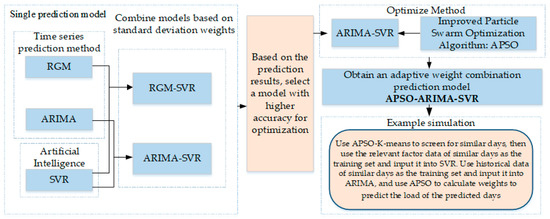
Figure 2.
The overall framework of load forecasting based on the hybrid forecasting model of adaptive inertial weights.
Modeling Procedure:
Step 1: Individual load forecasting models are constructed using both SVR and ARIMA methodologies. The sample training set is incorporated to determine the optimal parameters for each model.
Step 2: The sum of absolute prediction errors is adopted as the cost function for adaptive weight allocation in the hybrid forecasting model, expressed as follows:
Step 3: An improved PSO algorithm with adaptive inertia weight is employed to determine the optimal weighting coefficients for the hybrid forecasting model, ultimately yielding the optimized hybrid prediction model.
Step 3: The optimal weights for model combination are identified using adaptive inertia weight-based PSO, generating the final optimized hybrid predictor:
Step 4: The prediction accuracy of the APSO-ARIMA-SVR hybrid forecasting model is evaluated using two performance metrics: MAE and RMSE.
4. Case Study
4.1. Data Processing
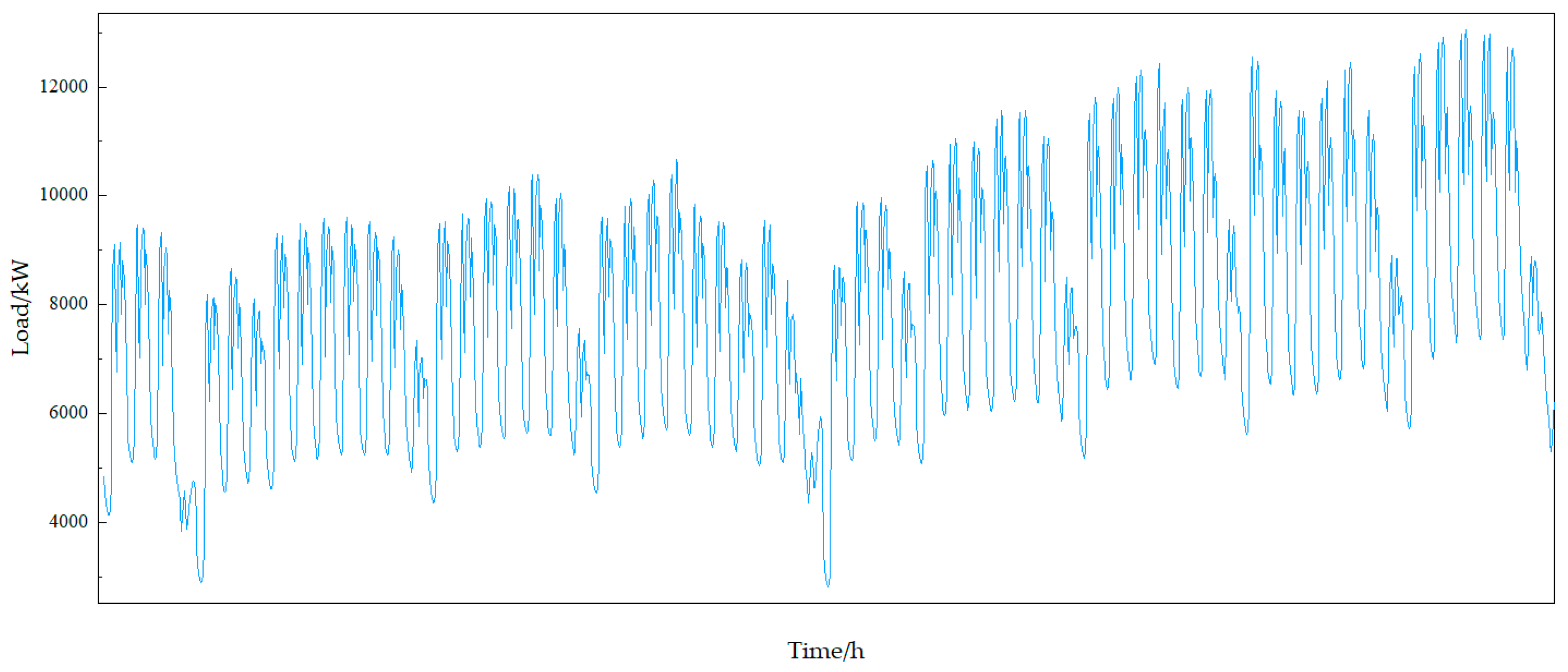
User load is influenced by external factors, exhibiting certain inherent patterns. The intrinsic patterns of user load mainly refer to the periodicity caused by the alternation between workdays and rest days, while the external influences such as ambient temperature, humidity, and weather types contribute to its continuity. Therefore, in load forecasting research, we should first analyze the variation patterns of user load and investigate its influencing factors, then normalize the historical data used as model inputs, and finally perform cluster analysis on the load data to select similar days. The dataset consists of 1464 load data points (with 1 h sampling interval) from the user side of a microgrid demonstration project in northwest China, covering the period from 1 May to 30 June 2015, along with recorded weather conditions and types in the region. The load fluctuation profile is illustrated in Figure 3.
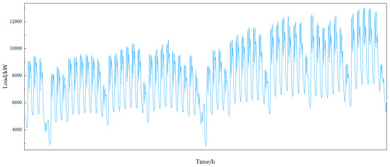
Figure 3.
User load profile from May to June.
4.1.1. Temporal Influencing Factors
Load fluctuation patterns are predominantly governed by residential activities and work schedules, exhibiting distinct periodicity corresponding to workday–weekend alternations. Weekly load variations demonstrate two characteristic patterns: workdays dominated by industrial and commercial operational loads resulting in higher and more stable demand profiles, and weekends showing reduced industrial contribution (though remaining predominant over residential loads) with consequently lower overall consumption levels. This systematic variation confirms the consistent elevation of workday loads compared to weekend demand, establishing fundamental periodicity in load characteristics.
4.1.2. Temperature Influencing Factors
User load profiles are significantly affected by environmental parameters and holiday patterns, where fluctuations in ambient temperature, precipitation, and snowfall directly influence electricity consumption, albeit with varying degrees of impact across different meteorological variables. These weather conditions primarily alter load characteristics by modulating human thermal comfort perceptions, which subsequently triggers adjustments in heating, cooling, and humidification equipment usage. This study specifically focuses on apparent temperature as the dominant meteorological determinant for load forecasting due to its proven correlation with residential and commercial energy consumption patterns.
The human body’s thermally neutral zone occurs at approximately 27 °C when considering ambient temperature alone, while additional environmental parameters including air humidity and wind speed collectively influence perceived comfort levels, necessitating the use of comprehensive apparent temperature indices for accurate environmental impact assessment. The mathematical formulation of this integrated comfort metric is presented below:
where k represents the apparent temperature index, Ta denotes ambient temperature (°C), Rh indicates relative humidity, and v signifies wind speed (m/s). The quantitative relationship between calculated apparent temperature values and corresponding thermal comfort levels is systematically classified in Table 6.
Table 6.
Human somatosensory index and comfort level.
The apparent temperature index demonstrates a strong correlation between perceptual indicators and ambient temperature, humidity, and wind speed, indicating that these meteorological parameters are critical factors influencing user load. Therefore, weather conditions—particularly ambient temperature, humidity, and wind speed—should be incorporated into predictive models for user load analysis.
4.1.3. Weather Type Influencing Factors
Weather classification, including sunny, cloudy, rainy, and snowy conditions, directly correlates with distinct combinations of ambient temperature and relative humidity that collectively influence electricity demand patterns. These meteorological variations systematically affect load fluctuations through multiple pathways. Given the inherent challenges in qualitative assessment of weather–load relationships, this study implements a quantitative weather classification framework as presented in Table 7.
Table 7.
Weather type.
4.1.4. Data Preprocessing
(1) Normalization
The min-max normalization method was employed to rescale all features to a fixed range [0, 1] using the formula
where x is the original value, and xmin and xmax represent the minimum and maximum values of the feature, respectively.
(2) Standardization
Z-score Standardization:
The z-score standardization was applied to transform the data to have zero mean and unit variance according to
where μ denotes the mean, and σ represents the standard deviation of the feature values.
4.1.5. Evaluation Method
(1) Mean Absolute Error (MAE)
(2) Mean Absolute Error (MAE)
where yi is the observed value, denotes the predicted value, ei represents the deviation between observed and predicted values, and m represents the sample size.
4.2. Adaptive Inertia-Weighted Hybrid Model for Short-Term Load Forecasting
Based on the characteristics of user load data and relevant influencing factors, this study constructs a short-term load forecasting model by employing K-means clustering analysis and the adaptive weighted hybrid prediction model. The specific implementation process is as follows:
- (1)
- The characteristics of historical user load and meteorological data were analyzed, followed by data preprocessing.
- (2)
- The dataset was classified into workdays and non-workdays, and then K-means clustering was applied to identify similar days.
- (3)
- Based on the forecasted meteorological conditions of the prediction day, corresponding historical load and weather data were selected from similar days as the training set, while using the predicted workday and non-workday as test sets.
- (4)
- Individual prediction models (RGM, ARIMA, and SVR) were employed for short-term load forecasting. The prediction errors were quantitatively calculated, followed by comprehensive model evaluation using standardized metrics.
- (5)
- Two hybrid models were developed by combining time series methods (RGM and ARIMA) with the machine learning approach (SVR) using standard deviation-based weighting. The RGM-SVR and ARIMA-SVR models were constructed for short-term load forecasting.
- (6)
- Prediction errors were computed, and based on the evaluation results, the more accurate and stable ARIMA-SVR hybrid model was selected for weight optimization.
- (7)
- The inertia weight of the PSO algorithm was improved by introducing elastic momentum, enhancing its search capability. The modified PSO (APSO) was then used to optimize the weights of the ARIMA-SVR model, ultimately establishing an adaptive hybrid forecasting model with elastic momentum, APSO-ARIMA-SVR.
- (8)
- The proposed adaptive weighted hybrid forecasting model APSO-ARIMA-SVR was trained and compared against individual prediction models (ARIMA, RGM, SVR), standard deviation-based combination models (ARIMA-SVR, RGM-SVR), and commonly used deep learning models (Transformer, LSTM) to verify its effectiveness. Prediction errors were calculated and evaluated using MAE, RMSE, and Diebold-Mariano test metrics. The comparative results demonstrated that the APSO-ARIMA-SVR model with adaptive weight optimization significantly outperformed all benchmark models in terms of both prediction accuracy and stability, as confirmed by rigorous statistical testing. This comprehensive validation establishes the proposed model as a robust solution for short-term load forecasting applications, combining the strengths of time series analysis, machine learning, and optimized ensemble techniques.
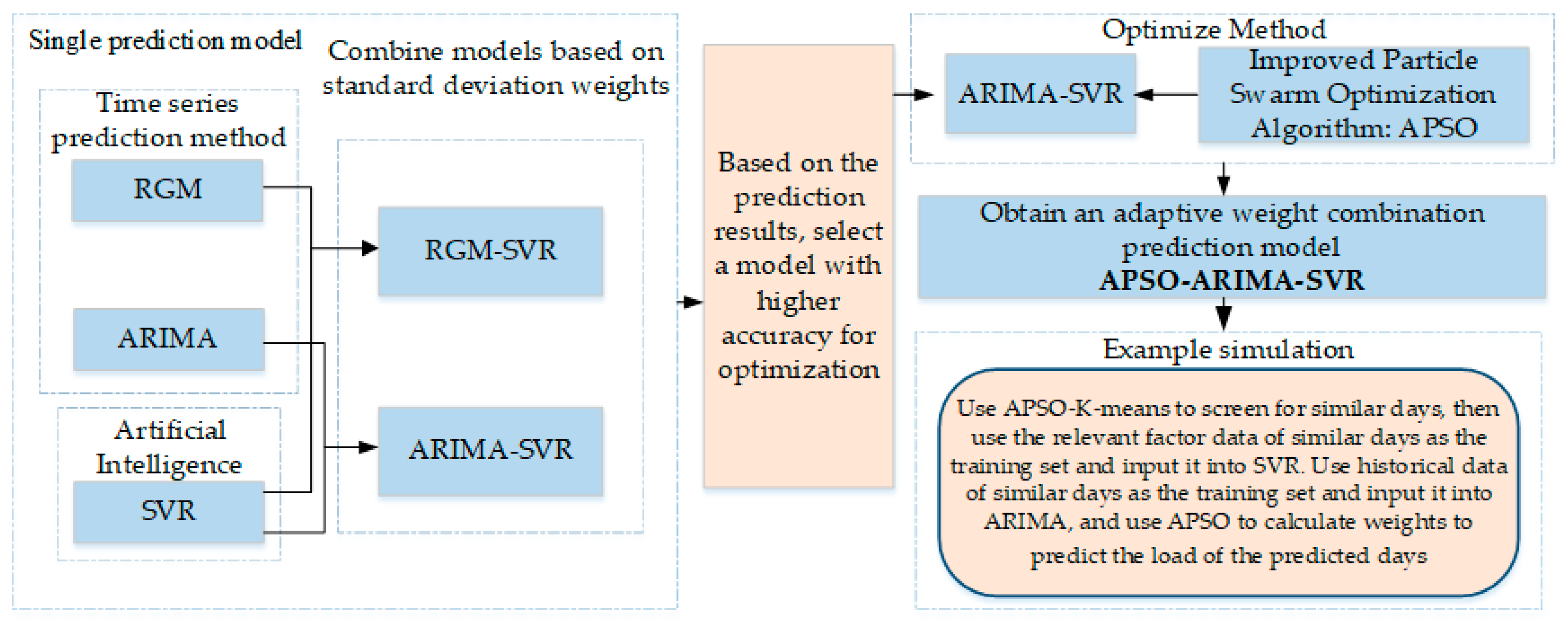
Figure 4 shows that the workflow of user load forecasting using the proposed adaptive weight hybrid model (APSO-ARIMA-SVR).
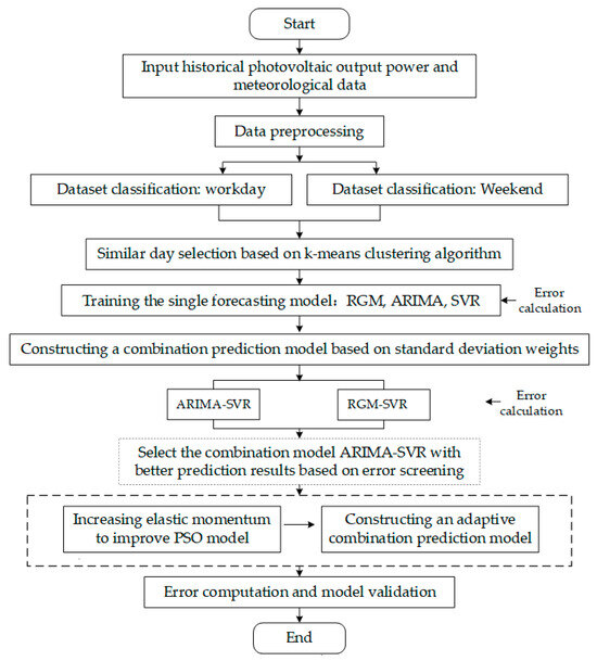
Figure 4.
Load forecasting process based on APSO-ARIMA-SVR model.
4.3. Results Analysis
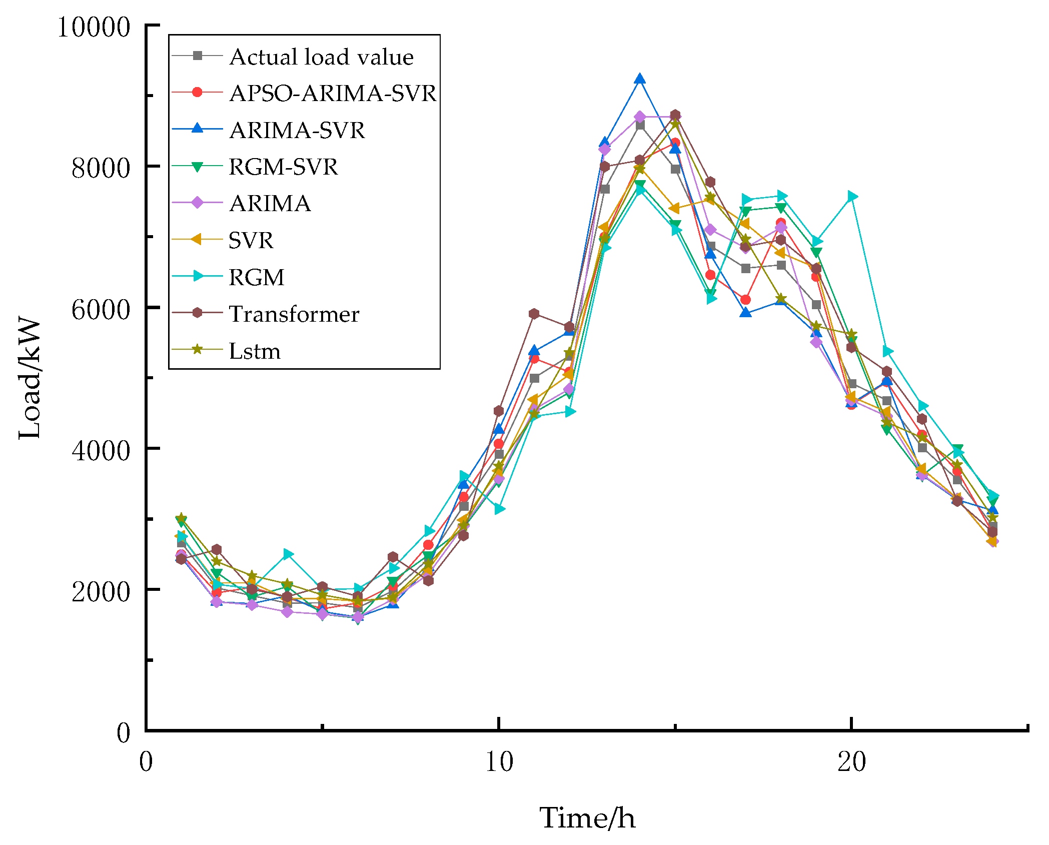
This study first classified the dataset into workdays and rest days and then selected the most similar days for prediction through cluster analysis. For the RGM and ARIMA model, historical load data from the five most similar days were used as training sets. For SVR, both historical load data and relevant meteorological factors from the five most similar days were selected as training inputs. The load data for prediction days (both workdays and rest days) served as test sets for the combined forecasting model. The prediction results are shown in Figure 5 and Figure 6, with model evaluation metrics presented in Table 8.
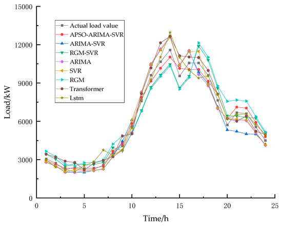
Figure 5.
Load forecasting results on weekdays.
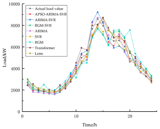
Figure 6.
Load forecasting results on weekend.
Table 8.
Model evaluation results.
This study further employed the APSO-ARIMA-SVR model as the benchmark and other comparative models as reference predictors for Diebold–Mariano (DM) testing, aiming to investigate whether statistically significant differences exist between the forecasting performance of the proposed APSO-ARIMA-SVR model with elastic momentum-based adaptive weighting and conventional approaches. The DM test results are summarized in Table 9.
Table 9.
The results of Diebold–Mariano test.
Figure 5 and Figure 6 show that the proposed hybrid forecasting model based on adaptive inertia weight (APSO-ARIMA-SVR) generates load predictions that most closely match the actual load data. The model shows superior performance compared to both standard deviation-based combination models (ARIMA-SVR, RGM-SVR) and individual models (ARIMA, RGM, SVR). Among the standard deviation-based approaches, the ARIMA-SVR model yields relatively better forecasting results.
As shown in Table 8, the proposed APSO-ARIMA-SVR model achieves the lowest prediction error and best fitting performance for workday load data. For weekend load data, while APSO-ARIMA-SVR still exhibits the smallest error, its prediction accuracy is relatively lower compared to workdays. The RGM demonstrates relatively high prediction accuracy during the initial three forecasting points. However, its prediction error increases significantly with extended forecasting horizons. For the small-sample dataset employed in this study, the RGM shows limited capability in capturing the fluctuation patterns of power load, rendering it unsuitable for power load forecasting applications.
As evidenced in Table 9, all forecasting models yielded p-values ≤ 0.05, demonstrating statistically significant differences between the proposed APSO-ARIMA-SVR model and each comparator model. The DM test results confirm that APSO-ARIMA-SVR achieves significantly superior forecasting performance at the 95% confidence level when compared against alternative approaches.
The dataset used in this study exhibits certain periodicity, resulting in relatively small weekend samples after similar-day screening. While the ARIMA model is suitable for periodic forecasting, SVR demonstrates stronger generalization capability and accommodates multi-factor samples without strict size limitations. Both Transformer and LSTM represent state-of-the-art deep learning models for forecasting applications. However, their performance is highly dependent on large-scale training datasets. The limited sample size employed in this study proved insufficient for these models to achieve adequate learning convergence, resulting in unstable predictions with significant error margins (MAE: 566.83, 511.72, RMSE: 633.56, 611.29). Therefore, the proposed APSO-ARIMA-SVR method is particularly appropriate for short-term load forecasting with small-sized, periodic datasets containing multiple relevant factors.
5. Conclusions
Accurate power load forecasting is crucial for power system dispatch, planning, and the construction of new-type power systems. This study proposes a hybrid short-term load forecasting method based on APSO-ARIMA-SVR, incorporating model optimization, parameter tuning, and training procedures. We conducted validation through simulation experiments using actual load measurement data from a microgrid demonstration project in northwest China, covering the operational period from 1 May to 30 June, the following conclusions:
- (1)
- Comparative simulations demonstrate that combined models (both standard deviation-based and adaptive weight-based) achieve superior generalization capability and higher accuracy compared to individual models.
- (2)
- The inertia weight in the particle swarm optimization algorithm is adaptively adjusted to propose an improved A-PSO model. Comparative experiments with other optimization algorithms demonstrate that the standard deviations of the optimization results for functions F1, F3, F4, F5, and F6 by the APSO algorithm are 1.00 × 10⁻¹⁰, 5.27 × 10⁻⁵, 2.39 × 10, 0.04 × 100, and 8.25 × 10⁻⁹, respectively. For most functions, the optimization accuracy of the APSO algorithm surpasses that of the PSO algorithm by several orders of magnitude, and it also outperforms traditional GWO, MFO, and WOA algorithms in terms of optimization precision. Notably, in solving continuous unimodal functions, the optimization accuracy of APSO is significantly superior to that of other algorithms.
- (3)
- We propose an adaptive weight hybrid forecasting model (APSO-ARIMA-SVR) by employing the APSO algorithm to optimize the parameter configuration and weight allocation of the ARIMA-SVR framework. Simulation case studies demonstrate that compared to the combined forecasting models RGM-SVR and ARIMA-SVR (based on standard deviation) as well as the single models ARIMA, RGM, and SVR, the adaptive weight combined forecasting model APSO-ARIMA-SVR achieves the best fitting performance and the lowest prediction error. The DM statistical test results indicate that, at a 95% confidence level, APSO-ARIMA-SVR significantly outperforms all other comparative models. Due to the small sample size of the dataset selected in this study, Transformer and LSTM may fail to fully learn the data patterns, resulting in relatively higher prediction errors. While the RGM model shows acceptable precision in initial prediction points, its performance deteriorates significantly with extended forecasting horizons due to inherent limitations in handling complex dataset characteristics, thus proving unsuitable for this application. The developed APSO-ARIMA-SVR framework effectively balances linear and nonlinear components through adaptive weight adjustment, demonstrating robust performance across varying load conditions while maintaining computational efficiency, thereby establishing itself as a recommended solution for short-term load forecasting tasks. In subsequent research, the model will be further optimized and trained/validated on more diverse types of datasets.
Author Contributions
Conceptualization, W.Z.; Funding acquisition, W.Z.; Formal analysis, W.Z., H.X. and J.Z.; Methodology, W.Z. and P.C.; Project administration, W.Z.; Writing—original draft: W.Z.; Writing–review and editing, W.Z.; Data curation, J.L.; Supervision, T.C. All authors have read and agreed to the published version of the manuscript.
Funding
This study is funded by the Humanities and Social Science Fund of Ministry of Education of China (No. 23YJCZH315), Natural Science Foundation for Young Scientists of Shanxi Province (No. 202303021212076), and National Natural Science Foundation of China (No. 72473104).
Data Availability Statement
The original contributions presented in the study are included in the article, further inquiries can be directed to the corresponding author.
Conflicts of Interest
The authors declare no conflicts of interest.
References
- Niu, D.; Wang, Y.; Wu, D. Power load forecasting using support vector machine and ant colony optimization. Expert Syst. Appl. 2010, 37, 2531–2539. [Google Scholar] [CrossRef]
- Hong, T.; Fan, S. Probabilistic electric load forecasting: A tutorial review. Int. J. Forecast. 2016, 32, 914–938. [Google Scholar] [CrossRef]
- Friedrich, L.; Afshari, A. Short-term Forecasting of the Abu Dhabi Electricity Load Using Multiple Weather Variables. Energy Procedia 2015, 75, 3014–3026. [Google Scholar] [CrossRef]
- Hamzacebi, C.; Es, H.A. Forecasting the annual electricity consumption of Turkey using an optimized grey model. Energy 2014, 70, 165–171. [Google Scholar] [CrossRef]
- Xiong, D.L.; Zhang, X.Y.; Yu, Z.W.; Zhang, X.F.; Long, H.M.; Chen, L.J. Development and application of an intelligent thermal state monitoring system for sintering machine tails based on cnn-lstm hybrid neural networks. J. Iron Steel Res. Int. 2025, 32, 52–63. [Google Scholar] [CrossRef]
- Wang, H.; Huang, S.; Yin, Y.; Gu, T. Short-term load forecasting based on pelican optimization algorithm and dropout long short-term memories–fully convolutional neural network optimization. Energies 2024, 17, 6115. [Google Scholar] [CrossRef]
- Singh, P.; Dwivedi, P. Integration of new evolutionary approach with artificial neural network for solving short term load forecast problem. Appl. Energy 2018, 217, 537–549. [Google Scholar] [CrossRef]
- Koen, R.; Holloway, J. Application of multiple regression analysis to forecasting South Africa’s electricity demand. J. Energy South. Afr. 2014, 25, 48–58. [Google Scholar] [CrossRef]
- Bianco, V.; Manca, O.; Nardini, S. Electricity consumption forecasting in Italy using linear regression models. Energy 2009, 34, 1413–1421. [Google Scholar] [CrossRef]
- Zhu, J.; Dong, H.; Zheng, W.; Li, S.; Huang, Y.; Xi, L. Review and prospect of data-driven techniques for load forecasting in integrated energy systems. Appl. Energy 2022, 321, 119269. [Google Scholar] [CrossRef]
- Xiong, P.P.; Dang, Y.G.; Yao, T.X. Optimal modeling and forecasting of the energy consumption and production in China. Energy 2014, 77, 623–634. [Google Scholar] [CrossRef]
- Xiong, X.; Hu, X.; Guo, H. A hybrid optimized grey seasonal variation index model improved by whale optimization algorithm for forecasting the residential electricity consumption. Energy 2021, 234, 121127. [Google Scholar] [CrossRef]
- Zeng, S.; Su, B.; Zhang, M.; Gao, Y.; Liu, J.; Luo, S.; Tao, Q. Analysis and forecast of China’s energy consumption structure. Energy Policy 2021, 159, 112630. [Google Scholar] [CrossRef]
- Karlsson, S. Forecasting with Bayesian vector autoregression. Handb. Econ. Forecast. 2013, 2, 791–897. [Google Scholar]
- Khan, S.; Alghulaiakh, H. ARIMA model for accurate time series stocks forecasting. Int. J. Adv. Comput. Sci. Appl. 2020, 11, 524–528. [Google Scholar] [CrossRef]
- Contreras, J.; Espinola, R.; Nogales, F.J.; Conejo, A.J. ARIMA models to predict next-day electricity prices. IEEE Trans. Power Syst. 2003, 18, 1014–1020. [Google Scholar] [CrossRef]
- Zhao, H.; Guo, S. An optimized grey model for annual power load forecasting. Energy 2016, 107, 272–286. [Google Scholar] [CrossRef]
- Box, G.E.P.; Jenkins, G. Time Series Analysis, Forecasting and Control; Holden-Day, Incorporated: San Francisco, CA, USA, 1990; pp. 238–242. [Google Scholar]
- Sen, P.; Roy, M.; Pal, P. Application of ARIMA for forecasting energy consumption and GHG emission: A case study of an Indian pig iron manufacturing organization. Energy 2016, 116, 1031–1038. [Google Scholar] [CrossRef]
- Abdel-Aal, R.E.; Al-Garni, A.Z. Forecasting monthly electric energy consumption in eastern Saudi Arabia using univariate time-series analysis. Energy 2014, 22, 1059–1069. [Google Scholar] [CrossRef]
- Wang, Q.; Li, S.; Li, R. China’s dependency on foreign oil will exceed 80% by 2030: Developing a novel NMGM-ARIMA to forecast China’s foreign oil dependence from two dimensions. Energy 2018, 163, 151–167. [Google Scholar] [CrossRef]
- Deng, J. Control problems of grey systems. J. Huazhong Inst. Technol. 1982, 10, 9–18. [Google Scholar]
- Wang, Q.; Song, X. Forecasting China’s oil consumption: A comparison of novel nonlinear-dynamic grey model (GM), linear GM, nonlinear GM and metabolism GM. Energy 2019, 183, 160–171. [Google Scholar] [CrossRef]
- Wang, Z.X.; Hao, P. An improved grey multivariable model for predicting industrial energy consumption in China. Appl. Math. Model. 2016, 40, 5745–5758. [Google Scholar] [CrossRef]
- Ding, S.; Hipel, K.W.; Dang, Y. Forecasting China’s electricity consumption using a new grey prediction model. Energy 2018, 149, 314–328. [Google Scholar] [CrossRef]
- Abisoye, B.O.; Sun, Y.; Zenghui, W. A survey of artificial intelligence methods for renewable energy forecasting: Methodologies and insights. Renew. Energy Focus 2024, 48, 100529. [Google Scholar] [CrossRef]
- Onwusinkwue, S.; Osasona, F.; Ahmad, I.A.I.; Anyanwu, A.C.; Dawodu, S.O.; Obi, O.C.; Hamdan, A. Artificial intelligence (AI) in renewable energy: A review of predictive maintenance and energy optimization. World J. Adv. Res. Rev. 2024, 21, 2487–2499. [Google Scholar] [CrossRef]
- Huang, X.; Li, Q.; Tai, Y.; Chen, Z.; Liu, J.; Shi, J.; Liu, W. Time series forecasting for hourly photovoltaic power using conditional generative adversarial network and Bi-LSTM. Energy 2022, 246, 123403. [Google Scholar] [CrossRef]
- Zhao, E.; Sun, S.; Wang, S. New developments in wind energy forecasting with artificial intelligence and big data: A scientometric insight. Data Sci. Manag. 2022, 5, 84–95. [Google Scholar] [CrossRef]
- Raza, M.Q.; Khosravi, A. A review on artificial intelligence based load demand forecasting techniques for smart grid and buildings. Renew. Sustain. Energy Rev. 2015, 50, 1352–1372. [Google Scholar] [CrossRef]
- Azadeh, A.; Babazadeh, R.; Asadzadeh, S.M. Optimum estimation and forecasting of renewable energy consumption by artificial neural networks. Renew. Sustain. Energy Rev. 2013, 27, 605–612. [Google Scholar] [CrossRef]
- Liu, M.; Cao, Z.; Zhang, J.; Wang, L.; Huang, C.; Luo, X. Short-term wind speed forecasting based on the Jaya-SVM model. Int. J. Electr. Power Energy Syst. 2020, 121, 106056. [Google Scholar] [CrossRef]
- Mengshu, S.; Yuansheng, H.; Xiaofeng, X.; Dunnan, L. China’s coal consumption forecasting using adaptive differential evolution algorithm and support vector machine. Resour. Policy 2021, 74, 102287. [Google Scholar] [CrossRef]
- Manzoor, H.U.; Khan, A.R.; Flynn, D.; Alam, M.M.; Akram, M.; Imran, M.A.; Zoha, A. Fedbranched: Leveraging federated learning for anomaly-aware load forecasting in energy networks. Sensors 2023, 23, 3570. [Google Scholar] [CrossRef]
- Fekri, M.N.; Grolinger, K.; Mir, S. Distributed load forecasting using smart meter data: Federated learning with Recurrent Neural Networks. Int. J. Electr. Power Energy Syst. 2022, 137, 107669. [Google Scholar] [CrossRef]
- Ba Dri, A.; Ameli, Z.; Birjandi, A.M. Application of Artificial Neural Networks and Fuzzy logic Methods for Short Term Load Forecasting. Energy Procedia 2012, 14, 1883–1888. [Google Scholar] [CrossRef]
- Wang, H.; Lei, Z.; Zhang, X.; Zhou, B.; Peng, J. A review of deep learning for renewable energy forecasting. Energy Convers. Manag. 2019, 198, 111799. [Google Scholar] [CrossRef]
- Aslam, S.; Herodotou, H.; Mohsin, S.M.; Javaid, N.; Ashraf, N.; Aslam, S. A survey on deep learning methods for power load and renewable energy forecasting in smart microgrids. Renew. Sustain. Energy Rev. 2021, 144, 110992. [Google Scholar] [CrossRef]
- Mamun, A.A.; Sohel, M.; Mohammad, N.; Sunny, M.S.H.; Dipta, D.R.; Hossain, E. A Comprehensive Review of the Load Forecasting Techniques Using Single and Hybrid Predictive Models. IEEE Access 2020, 8, 134911–134939. [Google Scholar] [CrossRef]
- Dedinec, A.; Filiposka, S.; Dedinec, A.; Kocarev, L. Deep belief network based electricity load forecasting: An analysis of Macedonian case. Energy 2016, 115, 1688–1700. [Google Scholar] [CrossRef]
- Dong, X.; Deng, S.; Wang, D. A short-term power load forecasting method based on k-means and SVM. J. Ambient. Intell. Humaniz. Comput. 2022, 13, 5253–5267. [Google Scholar] [CrossRef]
- Hu, S.; Xiang, Y.; Huo, D.; Jawad, S.; Liu, J. An improved deep belief network based hybrid forecasting method for wind power. Energy 2021, 224, 120185. [Google Scholar] [CrossRef]
- Wei, Y.; Zhang, H.; Dai, J.; Zhu, R.; Qiu, L.; Dong, Y.; Fang, S. Deep belief network with swarm spider optimization method for renewable energy power forecasting. Processes 2023, 11, 1001. [Google Scholar] [CrossRef]
- Chaturvedi, S.; Rajasekar, E.; Natarajan, S.; McCullen, N. A comparative assessment of SARIMA, LSTM RNN and Fb Prophet models to forecast total and peak monthly energy demand for India. Energy Policy 2022, 168, 113097. [Google Scholar] [CrossRef]
- Fang, W.; Chen, Y.; Xue, Q. Survey on research of RNN-based spatio-temporal sequence prediction algorithms. J. Big Data 2021, 3, 97. [Google Scholar] [CrossRef]
- Abumohsen, M.; Owda, A.Y.; Owda, M. Electrical load forecasting using LSTM, GRU, and RNN algorithms. Energies 2023, 16, 2283. [Google Scholar] [CrossRef]
- Sun, L.; Qin, H.; Przystupa, K.; Majka, M.; Kochan, O. Individualized short-term electric load forecasting using data-driven meta-heuristic method based on LSTM network. Sensors 2022, 22, 7900. [Google Scholar] [CrossRef]
- Kim, J.; Obregon, J.; Park, H.; Jung, J.Y. Multi-step photovoltaic power forecasting using transformer and recurrent neural networks. Renew. Sustain. Energy Rev. 2024, 200, 114479. [Google Scholar] [CrossRef]
- Giacomazzi, E.; Haag, F.; Hopf, K. Short-term electricity load forecasting using the temporal fusion transformer: Effect of grid hierarchies and data sources. In Proceedings of the 14th ACM International Conference on Future Energy Systems, Orlando, FL, USA, 20–23 June 2023; pp. 353–360. [Google Scholar]
- Galindo Padilha, G.A.; Ko, J.; Jung, J.J.; de Mattos Neto, P.S.G. Transformer-based hybrid forecasting model for multivariate renewable energy. Appl. Sci. 2022, 12, 10985. [Google Scholar] [CrossRef]
- Xu, H.; Hu, F.; Liang, X. A framework for electricity load forecasting based on attention mechanism time series depthwise separable convolutional neural network. Energy 2024, 299, 131258. [Google Scholar] [CrossRef]
- Singh, S.N.; Mohapatra, A. Data driven day-ahead electrical load forecasting through repeated wavelet transform assisted SVM model. Appl. Soft Comput. 2021, 111, 107730. [Google Scholar]
- Zeng, A.; Chen, M.; Zhang, L.; Xu, Q. Are transformers effective for time series forecasting? In Proceedings of the AAAI Conference on Artificial Intelligence, Washington, DC, USA, 7–14 February 2023; Volume 37, pp. 11121–11128. [Google Scholar]
- Wang, J.; Wang, Y.; Li, Z. A combined framework based on data preprocessing, neural networks and multi-tracker optimizer for wind speed prediction. Sustain. Energy Technol. Assess. 2020, 40, 100757. [Google Scholar] [CrossRef]
- Zheng, J.; Du, J.; Wang, B.; Klemeš, J.J.; Liao, Q.; Liang, Y. A hybrid framework for forecasting power generation of multiple renewable energy sources. Renew. Sustain. Energy Rev. 2023, 172, 113046. [Google Scholar] [CrossRef]
- Hajirahimi, Z.; Khashei, M. Hybridization of hybrid structures for time series forecasting: A review. Artif. Intell. Rev. 2023, 56, 1201–1261. [Google Scholar] [CrossRef]
- Song, C.; Fu, X. Research on different weight combination in air quality forecasting models. J. Clean. Prod. 2020, 261, 121169. [Google Scholar] [CrossRef]
- Wang, Y.M.; Luo, Y. Integration of correlations with standard deviations for determining attribute weights in multiple attribute decision making. Math. Comput. Model. 2010, 51, 1–12. [Google Scholar] [CrossRef]
- Qu, W.; Li, J.; Song, W.; Li, X.; Zhao, Y.; Dong, H.; Qi, Y. Entropy-weight-method-based integrated models for short-term intersection traffic flow prediction. Entropy 2022, 24, 849. [Google Scholar] [CrossRef]
- Raziani, S.; Ahmadian, S.; Jalali, S.M.J.; Chalechale, A. An efficient hybrid model based on modified whale optimization algorithm and multilayer perceptron neural network for medical classification problems. J. Bionic Eng. 2022, 19, 1504–1521. [Google Scholar] [CrossRef]
- Yang, S.S.; Yang, X.H.; Jiang, R.; Zhang, Y.C. New optimal weight combination model for forecasting precipitation. Math. Probl. Eng. 2012, 1, 376010. [Google Scholar] [CrossRef]
- Wang, C.; Lin, H.; Hu, H.; Yang, M.; Ma, L. A hybrid model with combined feature selection based on optimized VMD and improved multi-objective coati optimization algorithm for short-term wind power prediction. Energy 2024, 293, 130684. [Google Scholar] [CrossRef]
- Wang, Y.; Wang, D.; Tang, Y. Clustered hybrid wind power prediction model based on ARMA, PSO-SVM, and clustering methods. IEEE Access 2020, 8, 17071–17079. [Google Scholar] [CrossRef]
- Tang, T.; Jiang, W.; Zhang, H.; Nie, J.; Xiong, Z.; Wu, X.; Feng, W. GM (1, 1) based improved seasonal index model for monthly electricity consumption forecasting. Energy 2022, 252, 124041. [Google Scholar] [CrossRef]
- Box, G.E.; Pierce, D.A. Distribution of residual autocorrelations in autoregressive-integrated moving average time series models. J. Am. Stat. Assoc. 1970, 65, 1509–1526. [Google Scholar] [CrossRef]
- Cortes, C.; Vapnik, V. Support vector machine. Mach. Learn. 1995, 20, 273–297. [Google Scholar] [CrossRef]
- Aburomman, A.A.; Reaz, M.B.I. A novel SVM-kNN-PSO ensemble method for intrusion detection system. Appl. Soft Comput. 2016, 38, 360–372. [Google Scholar] [CrossRef]
- Kennedy, J.; Eberhart, R. Particle swarm optimization. In Proceedings of the IEEE International Conference on Neural Networks, Perth, WA, Australia, 27 November–1 December 1995; Volume 4, pp. 1942–1948. [Google Scholar]

Disclaimer/Publisher’s Note: The statements, opinions and data contained in all publications are solely those of the individual author(s) and contributor(s) and not of MDPI and/or the editor(s). MDPI and/or the editor(s) disclaim responsibility for any injury to people or property resulting from any ideas, methods, instructions or products referred to in the content. |
© 2025 by the authors. Licensee MDPI, Basel, Switzerland. This article is an open access article distributed under the terms and conditions of the Creative Commons Attribution (CC BY) license (https://creativecommons.org/licenses/by/4.0/).