Techno-Economic Assessment of Hydrogen-Based Power-to-Power Systems: Operational Strategies and Feasibility Within Energy Communities

Abstract

In the context of the evolving energy landscape, the need to harness renewable energy sources (RESs) has become increasingly imperative. Within this framework, hydrogen emerges as a promising energy storage vector, offering a viable solution to the flexibility challenges caused by the inherent variability of RESs. This work investigates the feasibility of integrating a hydrogen-based energy storage system within an energy community in Barcelona, using surplus electricity from photovoltaic (PV) panels. A power-to-power configuration is modelled through a comprehensive methodology that determines optimal component sizing, based on high-resolution real-world data. This analysis explores how different operational strategies influence the system’s cost-effectiveness. The methodology is thus intended to assist in the early-stage decision-making process, offering a flexible approach that can be adapted to various market conditions and operational scenarios. The results show that, under the current conditions, the combination of PV generation, energy storage, and low-cost grid electricity purchases yield the most favourable outcomes. However, in a long-term perspective, considering projected cost reductions for hydrogen technologies, strategies including energy sales back to the grid become more profitable. This case study offers a practical example of balancing engineering and economic considerations, providing replicable insights for designing hydrogen storage systems in similar energy communities.

1. Introduction

The rapid expansion of variable renewable energy sources (RESs)—i.e., solar photovoltaics and wind—has been decisive for achieving national and European decarbonization targets. Yet the intrinsic intermittency of these assets intensifies the need for flexible resources that can balance generation and demand across multiple time-scales and grid levels. Renewable energy communities (RECs) have therefore emerged as a promising framework in which groups of consumers and prosumers cooperatively generate, share and manage electricity within a defined area. By increasing local RES penetration, lowering network losses and fostering public acceptance of clean energy projects, RECs can accelerate the energy transition and democratize its benefits [1,2]. Nevertheless, high self-consumption targets and peak-shaving requirements oblige RECs to adopt effective storage- or demand-side measures; without them, surplus production is curtailed or exported at unfavourable tariffs, eroding economic viability. Conventional battery storage delivers high round-trip efficiencies but becomes costly and bulky for multi-day or seasonal balancing. This limitation has stimulated growing interest in long-duration, modular storage options that can couple electricity with other energy vectors.

Against this backdrop, hydrogen has emerged as a versatile energy carrier capable of supporting deep decarbonization across power, mobility, industry and heating sectors [3,4,5,6]. Ambitious national and regional roadmaps [7] aim to accelerate the deployment of renewable (“green”) hydrogen produced by electrolysis. Because of its high specific energy and long storage duration, hydrogen complements batteries by shifting surplus electricity across days or seasons; it can also serve as feedstock, transport fuel or a thermal source, thereby extending the sector-coupling potential of RECs.

A typical power-to-power (PtP) hydrogen chain comprises an electrolyzer that converts excess renewable electricity into H₂, a compressed gas storage vessel and a fuel cell that reconverts the gas into electricity during deficit periods. Although its round-trip efficiency is lower than that of batteries, modelling studies confirm that hydrogen-based PtP storage can substantially raise REC self-sufficiency and unlock flexibility revenues, especially where surplus generation would otherwise be curtailed. For instance, Raimondi and Spazzafumo [8] simulated a grid-connected hydrogen-based PtP scheme in an Italian REC and showed how the system increased users’ autarchy from 69% to 84%, albeit with current technology costs constraining economic viability. Ferrara et al. [9] optimized the scheduling of PV, battery, electrolyzer and fuel cell assets to maximize self-consumption, hydrogen production for external sale and distribution-network services. Further contributions examined risk-aware operation [10], anion exchange membrane electrolyzer optimization for distributed communities [11] and participation of PtP assets in Italy’s UVAM (Virtually Aggregated Mixed Units) flexibility program [12]. While these contributions highlight hydrogen’s technical potential, they also underline that its profitability depends on continued cost reductions, favourable incentives, and adequate access to energy markets.

Hydrogen storage becomes particularly attractive in remote or off-grid microgrids, where grid reinforcement is impractical. Aydin and Dincer [13] developed a life cycle assessment model for remote communities in Canada, showing that hydrogen-based renewable systems reduce global warming potential by up to 98.7% compared to diesel-only systems. Focusing on island contexts, Superchi et al. [14] demonstrated that seasonal green hydrogen storage coupled with batteries can reduce the levelized cost of required energy compared to battery-only energy storage. A conceptual study by Uyar and Beşikci [15] discussed how hydrogen and electricity production from renewable resources will contribute to the transition to 100% renewable energies. Complementing these works, Jin et al. [16] integrated a small-hydropower plant with battery and hydrogen storage, revealing that batteries’ levelized cost of storage could be 10 times higher than hydrogen, highlighting the need for hybrid storage solutions.

Finally, Garner and Dehouche [17] optimized the component sizes of a hybrid H₂–battery system for a Spanish island, finding an optimal design able to deliver 94–96% self-consumption while cutting the carbon intensity by 72% compared to the grid. Furthermore, their sensitivity analysis shows the hybrid battery-plus-hydrogen layout outperforms battery-only or H₂-only options in the cost vs. emissions Pareto space, confirming the complementarity of short- and long-duration storage. Together, these studies confirm that hydrogen’s high energy density and seasonal capability make it indispensable, coupled with short-term battery storage, for achieving energy autonomy and diesel displacement in isolated microgrids. Nastasi and Mazzoni [18] further showed that introducing self-consumption incentives and updated (post-COVID) electricity tariffs in a hydrogen–battery renewable energy community enables positive net present value for both storage solutions. Hydrogen storage is found to be optimal by 2030–2040, becoming cost-competitive with batteries in most scenarios due to lower investment cost per kWh. Analyses from the REMOTE project likewise demonstrate that hydrogen paired with batteries attains near 100% renewable supply without excessive oversizing of PV–wind capacity [19,20].

Novelty and Contribution of This Work

Despite growing interest in hydrogen storage for renewable energy communities, current research still exhibits critical shortcomings. First, most operational studies rely on hourly time-steps, a resolution that does not capture the fast dynamics of Proton Exchange Membrane (PEM) electrolyzers and fuel cells. Second, many techno-economic assessments treat the electrolysis and fuel cell as static blocks with fixed efficiencies, overlooking part-load penalties. Third, studies that integrate plant simulation with economic analysis often adopt a single control strategy, offering limited insight into how alternative operating logics influence profitability under real-world conditions.

In this context, this study presents a comprehensive simulation framework that couples dynamic electrochemical models of a PEM electrolyzer and fuel cell with a high-level techno-economic module able to test multiple operating strategies within an REC. Calibrated on second-resolution solar generation and load data from an industrial energy community in Barcelona, the model captures the full power-to-hydrogen-to-power chain—electrolysis, hydrogen storage and reconversion—in realistic operating conditions.

The framework pursues a dual objective: (i) to provide an energetically accurate representation of PEM-based PtP systems and (ii) to assess their economic feasibility under real consumption patterns and market signals. By bridging detailed technical behaviour with cost-optimization analysis, the tool delivers practical guidance for the sustainable deployment of hydrogen storage in urban and industrial communities and can be readily replicated in similar settings.

The paper is organized as follows. Section 2 details the case study, the dynamic modelling approach and the techno-economic formulation, including data sources and scenario definitions. Section 3 and Section 4 present the energetic and economic results, discuss sensitivity analyses on component sizing and costs, and compare the proposed control strategies. Finally, Section 5 summarizes the principal findings, acknowledges model limitations and outlines directions for future research.

2. Materials and Methods

The initial part of the work presents a simplified model of a power-to-power system, including an electrolyzer, a hydrogen storage tank and a fuel cell. The entire model is developed within a MATLAB/Simulink^® (R2024a) environment, which enables the simulation of the dynamic behaviour of the system’s components. This modelling approach provides a detailed and accurate representation of the time-dependent interactions among the various elements, offering a flexible framework for system design, analysis and performance optimization.

The chosen simulation time step has been deliberately chosen to capture the natural fluctuations in PV generation and load demand. These short-term variations are critical for accurately reflecting the behaviour of key components such as the electrolyzer and fuel cell, particularly their start-up events and dispatch dynamics. A coarser resolution (e.g., hourly) would smooth out these fluctuations, potentially introducing errors in the energy balance and masking important system behaviours like surplus peaks or deficit spikes. The one-second resolution strikes a good balance between accuracy and computational cost, ensuring that both technical performance and economic comparisons across control strategies are realistically represented.

The following chapter is divided into five sections. The first three sections describe the key components of the system (the electrolyzer, the hydrogen tank and the fuel cell). Each section explains the function of the respective component within the system and its operational characteristics. Section 2.4 outlines the main assumptions and datasets employed in the simulation. Finally, the last subsection introduces and discusses the different operational strategies considered for the hydrogen-based energy storage system.

2.1. Electrolyzer Model

The focus is placed exclusively on the Proton Exchange Membrane (PEM) electrolyzer technology. After comparing this with an alkaline electrolyzer model, it was concluded that the PEM electrolyzer offers higher efficiency and better dynamic behaviour. As a result, the alkaline electrolyzer model has been excluded from further discussion in this work.

Model assumptions are listed as follows:

• A steady-state electrochemical mechanism for the electrolyzer is used, implying that the system exhibits an instantaneous response to input changes, with no time delays. This assumption is supported by the fact that typically, the response time of PEM electrolyzers is rapid, approximately 50 ms for a PEM stack [21]; thus, this simplified approach is justified.
• The electrolyzer is assumed to be isothermal (average cell temperature is considered); thus, the thermodynamic model is considered static as well.
• Gases are approximated as ideal gases.

Thermodynamic and electrochemical [22] considerations are discussed below.

The minimum voltage needed to be applied between the electrodes of each cell is the reversible voltage, and it is calculated taking into consideration the partial pressures of hydrogen, oxygen and water ($p_{H_2}$, $p_{O_2}$, $p_{H_{2}O}$).

$$V_{rev}=V_{rev,T}°+{\displaystyle \frac{R\cdot T}{z\cdot F}}\ln \left({\displaystyle \frac{p_{H_2}\cdot p_{O_2}^{\frac{1}{2}}}{p_{H_{2}O}}}\right)$$

(1)

The first term $V_{rev,T}°$ is also obtained as a function of temperature ($T$):

$$V_{rev,T}°=1.5241-1.2261\cdot {10}^{-3}\cdot T+1.1858\cdot {10}^{-5}\cdot T\cdot \mathit{ln}T+5.6692\cdot {10}^{-7}\cdot T^2$$

(2)

$R$, $z$ and $F$ are the universal gas constant, the number of electrons transferred per reaction and the Faraday constant, respectively.

The cell voltage is given by the sum of the reversible voltage, the activation, the ohmic and the concentration overvoltages. The last term will be neglected since it is not significant at moderate current densities [22].

The activation overvoltage (${\mathsf{\eta }}_{act},\mathrm{i}\mathrm{n}\mathrm{V}$) is calculated, respectively, for the anode and the cathode through the Butler–Volmer equation:

$${\mathsf{\eta }}_{act}={\displaystyle \frac{R\cdot T}{\alpha \cdot F}}\cdot \mathrm{arcsinh}\left({\displaystyle \frac{i}{2\cdot i_0}}\right)$$

(3)

where $\alpha$ is the charge transfer coefficient, $i$ corresponds to the current density and $i_0$ represents the exchange current density. The final values used in the model are listed in Table 1.

The ohmic overpotential (${\mathsf{\eta }}_{ohm},\mathrm{i}\mathrm{n}\mathrm{V}$) is calculated as the product between the ohmic resistance of each cell in the stack ($R_{cell},\mathrm{i}\mathrm{n}\mathsf{\Omega }$) and the current ($I,\mathrm{i}\mathrm{n}\mathrm{A}$). Since the cell is composed of plates and a membrane, the equivalent resistance can be defined as the sum of the resistance of electrodes and the one due to the membrane as follows:

$${\mathsf{\eta }}_{ohm}=R_{cell}\cdot I=\left(R_{an}+R_{cat}+R_{mem}\right)\cdot I$$

(4)

The ohmic resistance of the membrane ($R_{mem},\mathrm{in}\mathsf{\Omega }$) is bigger than the one measured at the electrodes [23]; so in this model, only the former is considered using the expression below:

$$R_{mem}={\displaystyle \frac{{\delta }_{mem}}{{\sigma }_{mem}}}$$

(5)

The ${\delta }_{mem}$ term represents the thickness of the electrolyte membrane, and its value is reported in Table 1, while the ${\sigma }_{mem}$ is the conductivity of the membrane itself, which can be calculated through the following expression [22,23]:

$${\sigma }_{mem}=\left(0.00514\cdot \lambda -0.00326\right)\cdot \exp \left[1268\cdot \left({\displaystyle \frac{1}{303}}-{\displaystyle \frac{1}{T}}\right)\right]$$

(6)

The $\lambda$ term is the degree of humidification of the membrane, which is generally assumed to be in the range 14–21 [23] in the case of an electrolyzer. For this study, a value of 20 is chosen.

The model employed in this study builds upon the foundational work of H. Görgun [24], which was later subjected to dynamic testing by Yigit et al. [22]. Each module—anode, cathode and membrane—is developed independently, but they are tightly interconnected, as the output from one module often serves as the input for another. The model adheres to the principle of mass (or mole) conservation at both the anode and cathode, while the membrane is characterized by water transport mechanisms, including electro-osmotic drag and diffusion processes. These interactions ensure an accurate representation of the physical processes occurring within the system.

2.1.1. Anode Module

The anode module is responsible for water separation and the half-reaction of oxidation, where oxygen is generated and water is consumed. The system dynamics are accurately captured by the governing Equations (7) and (9), which, respectively, describe the rate of oxygen generation ($F_{O_2}$) and the rate of water consumption ($F_{H_{2}O,a}$). These equations reflect the mass balances and reaction kinetics occurring within the anode, ensuring that the behaviour of key species, such as oxygen and water, is properly quantified under dynamic operating conditions.

$$F_{O_2}=F_{O_2,ai}-F_{O_2,ao}+F_{o_2,g}$$

(7)

where

$F_{O_2,ai}$—inlet molar flow of oxygen, $\mathrm{m}\mathrm{o}\mathrm{l}{\mathrm{s}}^{-1}$, which is assumed to be equal to zero since water is the only input on the anode side;

$F_{O_2,ao}$—outlet molar flow of oxygen, $\mathrm{m}\mathrm{o}\mathrm{l}{\mathrm{s}}^{-1}$;

$F_{o_2,g}$—rate of oxygen generated, $\mathrm{m}\mathrm{o}\mathrm{l}{\mathrm{s}}^{-1}$, obtained through the general Faraday law:

$$F_{o_2,g}={\displaystyle \frac{n_c\cdot I}{4\cdot F}}$$

(8)

where $n_c$ corresponds to the number of cells. The dynamic flow of water in anode is described through the equation of mass conservation:

$$F_{H_{2}O,a}=F_{H_{2}O,ai}-F_{H_{2}O,ao}-F_{H_{2}O,eod}-F_{H_{2}O,diff}-F_{H_{2}O,conv}$$

(9)

where

$F_{H_{2}O,ai}$—inlet molar flow of water, $\mathrm{m}\mathrm{o}\mathrm{l}{\mathrm{s}}^{-1}$;

$F_{H_{2}O,ao}$—outlet molar flow of water, $\mathrm{m}\mathrm{o}\mathrm{l}{\mathrm{s}}^{-1}$;

$F_{H_{2}O,eod}$—electro-osmotic drag, since the water is dragged to the cathode by the hydrogen ions, $\mathrm{m}\mathrm{o}\mathrm{l}{\mathrm{s}}^{-1}$;

$F_{H_{2}O,diff}$—diffusion flow due to water concentration gradient across the membrane;

$F_{H_{2}O,conv}$—pressure gradient (convection) flow.

The inlet molar flow of water is a defined value that is continuously provided to the anode, and it is assumed to be proportional to the water required to make the reaction possible through the Faraday law:

$$F_{H_{2}O,ai}={\displaystyle \frac{n_c\cdot I}{2\cdot F}}$$

(10)

The partial pressures of oxygen and water in the anode can be calculated through the ideal gas law. Finally, the total anode pressure is given by the sum of the partial pressures.

Oxygen and water mole fractions at the anode outlet are obtained, respectively, as

$$y_{O_2}={\displaystyle \frac{p_{O_2}}{P_a}}$$

(11)

$$y_{H_{2}O,a}={\displaystyle \frac{p_{H_{2}O,an}}{P_a}}$$

(12)

Molar fractions are needed to compute the outlet flows of oxygen and water on the anode side, that, respectively, are

$${F_{O_2,ao}=y}_{O_2}\cdot F_{ao}$$

(13)

$${F_{H_{2}O,ao}=y}_{H_{2}O,a}\cdot F_{ao}$$

(14)

where $F_{ao}\left(\mathrm{m}\mathrm{o}\mathrm{l}{\mathrm{s}}^{-1}\right)$ is the total amount of out-flow, obtained by the difference between total pressure at anode and external standard pressure, multiplied by the anode outlet flow coefficient $k_{ao}$:

$$F_{ao}=k_{ao}\cdot \left(P_a-P_{a,0}\right)$$

(15)

2.1.2. Cathode Module

The second module is the one that regards the cathode electrode, where the half-reaction of hydrogen reduction occurs. Consequently, the species present are hydrogen and water. The balance of flows is analyzed in the following equations, which show the rate of generation of hydrogen and the water hold-ups:

$$F_{H_2}=F_{H_2,ci}-F_{H_2,co}+F_{H_2,g}$$

(16)

where

$F_{H_2,ci}$—inlet molar flow of hydrogen, $\mathrm{m}\mathrm{o}\mathrm{l}{\mathrm{s}}^{-1}$, which is assumed to be equal to zero since there is no inlet flow on the cathode side;

$F_{H_2,co}$—outlet molar flow of hydrogen, $\mathrm{m}\mathrm{o}\mathrm{l}{\mathrm{s}}^{-1}$;

$F_{H_2,g}$—rate of hydrogen generated, $\mathrm{m}\mathrm{o}\mathrm{l}{\mathrm{s}}^{-1}$, obtained through the general Faraday law:

$$F_{H_2,g}={\displaystyle \frac{n_c\cdot I}{2\cdot F}}$$

(17)

The dynamic flow of water in the cathode is described similarly to (9), again through the equation of mass conservation:

$$F_{H_{2}O,c}=F_{H_{2}O,ci}-F_{H_{2}O,co}+F_{H_{2}O,eod}+F_{H_{2}O,diff}+F_{H_{2}O,conv}$$

(18)

where

$F_{H_{2}O,ci}$—inlet molar flow of water, $\mathrm{m}\mathrm{o}\mathrm{l}{\mathrm{s}}^{-1}$, which is assumed to be equal to zero, since there is no inflow on the cathode side;

$F_{H_{2}O,co}$—outlet molar flow of water, $\mathrm{m}\mathrm{o}\mathrm{l}{\mathrm{s}}^{-1}$;

$F_{H_{2}O,eod}$—electro-osmotic drag, since the water is dragged to the cathode by the hydrogen ions, $\mathrm{m}\mathrm{o}\mathrm{l}{\mathrm{s}}^{-1}$;

$F_{H_{2}O,diff}$—diffusion flow;

$F_{H_{2}O,conv}$—convection.

The partial pressures of hydrogen and water in the cathode can be calculated again through the ideal gas law, and the total cathode pressure is then obtained.

Equations (11)–(15) are also implemented for the cathode, where the oxygen is substituted by hydrogen.

2.1.3. Membrane Module

The last module is the one related to the membrane, where the hydrogen ions pass through. However, the water can also cross the membrane because it is transported by convection, diffusion and the electro-osmotic drag. The convection is generated by a difference in pressure between the two electrodes, but since, in this case, the anode and cathode are assumed to be at the same pressure, it will be neglected.

Water diffusion is given from Fick’s first law as follows:

$$F_{H_{2}O,diff}=D_w\cdot {\displaystyle \frac{\left(C_{wc}-C_{wa}\right)}{t_m}}\cdot A\cdot n_{cells}$$

(19)

where $D_w$ is the water diffusion coefficient, $C_{wc}$ and $C_{wa}$ are the water concentrations for the cathode and anode surfaces of the membrane and $t_m$ is the thickness of the membrane. However, the hypothesis about the equilibrium of the membrane with the liquid water on both sides of the cell has been established, so the difference between water concentrations is assumed to be null and, consequently, the $F_{H_{2}O,diff}$ can also be neglected.

The last contribution that has to be taken into consideration within the membrane is related to the phenomenon of the electro-osmotic drag [25], which is obtained through the following equation:

$$F_{H_{2}O,eod}=n_d\cdot {\displaystyle \frac{n_{cells}\cdot I}{F}}$$

(20)

In fact, it has been tested that every proton is able to transport some molecules of water from the anode to the cathode, and this is represented by the electro-osmotic drag coefficient $n_d\left(\mathrm{m}\mathrm{o}{\mathrm{l}}_{{\mathrm{H}}_2\mathrm{O}}\mathrm{m}\mathrm{o}{\mathrm{l}}_{{\mathrm{H}}^{+}}^{-1}\right)$, whose value can be calculated in different ways as explained by Li et al. [25]. The one used in this work is given by Equation (21), which shows a linear dependence on the temperature (in K).

$$n_d=0.016\cdot T-2.89556$$

(21)

2.1.4. Model Implementation

The model described up to now shows a molar balance in the anode and cathode without specifying the state of the water inside. In fact, using the equations already mentioned, it is understandable that the total water is considered to be vapour by Yigit et al. [22]. This is a common approach in the literature, as shown also by Correa et al. [26]. However, this strong simplification does not take into account the fact that the PEM electrolyzer actually works with liquid water, since the relatively low temperature and pressure do not allow it to reach full gasification. For this reason, changes are applied to the previous model, applying some changes to the equations mentioned above.

Starting again from the anode side, the molar balance, Equation (9), of water in the anode becomes

$$F_{H_{2}O,a}=F_{H_{2}O,ai,liq}-F_{H_{2}O,ao,liq}-F_{H_{2}O,ao,gas}-F_{H_{2}O,eod}-F_{H_{2}O,diff}-F_{H_{2}O,conv}$$

(22)

It is worth underlining that the inlet water is provided as liquid, while the water exiting can be distinguished between liquid and vapour. Indeed, when the saturation pressure is reached, the water becomes liquid, so the amount of liquid water exiting the anode also has to be established. On the cathode side, the same assumptions are made, and the molar balance equation described in (18) changes into

$$F_{H_{2}O,c}=F_{H_{2}O,ci}-F_{H_{2}O,co,liq}-F_{H_{2}O,co,gas}+F_{H_{2}O,eod}+F_{H_{2}O,diff}+F_{H_{2}O,conv}$$

(23)

The main assumptions are related to the input parameters needed. Table 1 shows the values chosen for the electrolyzer model.

Table 1. Input parameters for the electrolyzer model.

Symbol	Parameter	Value	Ref.
Anode
$P_{an}$	Anode total pressure	$7\mathrm{b}\mathrm{a}\mathrm{r}$	[23]
$i_{0,an}$	Anode exchange current	${10}^{-12}\mathrm{A}{\mathrm{c}\mathrm{m}}^{-2}$	[23,27]
${\alpha }_{an}$	Anode charge transfer coefficient	$2$	[23,27]
$k_{ao}$	Anode outlet flow coefficient	$2.5\cdot {10}^{-7}$
Cathode
$i_{0,cat}$	Cathode exchange current	${10}^{-3}\mathrm{A}{\mathrm{c}\mathrm{m}}^{-2}$	[23,27]
${\alpha }_{cat}$	Cathode charge transfer coefficient	$0.5$	[23,27]
$k_{co}$	Cathode outlet flow coefficient	$2\cdot {10}^{-6}$
Other parameters of the electrolyzer
$F$	Faraday constant	96,485.3 $\mathrm{A}{\mathrm{m}\mathrm{o}\mathrm{l}}^{-1}$	[28]
$R$	Universal gas constant	$8.314\mathrm{J}{\mathrm{m}\mathrm{o}\mathrm{l}}^{-1}{\mathrm{K}}^{-1}$	[28]
$N$	Number of cells	$380$
$T$	Temperature	80 °C
$p_0$	Standard atmospheric pressure	101,325 $\mathrm{b}\mathrm{a}\mathrm{r}$
${\delta }_{mem}$	Thickness of electrolyte membrane (Nafion 117 PFSA DuPont)	$78\cdot {10}^{-4}\mathrm{c}\mathrm{m}$	[29]

Table 1. Input parameters for the electrolyzer model.

Symbol	Parameter	Value	Ref.
Anode
$P_{an}$	Anode total pressure	$7\mathrm{b}\mathrm{a}\mathrm{r}$	[23]
$i_{0,an}$	Anode exchange current	${10}^{-12}\mathrm{A}{\mathrm{c}\mathrm{m}}^{-2}$	[23,27]
${\alpha }_{an}$	Anode charge transfer coefficient	$2$	[23,27]
$k_{ao}$	Anode outlet flow coefficient	$2.5\cdot {10}^{-7}$
Cathode
$i_{0,cat}$	Cathode exchange current	${10}^{-3}\mathrm{A}{\mathrm{c}\mathrm{m}}^{-2}$	[23,27]
${\alpha }_{cat}$	Cathode charge transfer coefficient	$0.5$	[23,27]
$k_{co}$	Cathode outlet flow coefficient	$2\cdot {10}^{-6}$
Other parameters of the electrolyzer
$F$	Faraday constant	96,485.3 $\mathrm{A}{\mathrm{m}\mathrm{o}\mathrm{l}}^{-1}$	[28]
$R$	Universal gas constant	$8.314\mathrm{J}{\mathrm{m}\mathrm{o}\mathrm{l}}^{-1}{\mathrm{K}}^{-1}$	[28]
$N$	Number of cells	$380$
$T$	Temperature	80 °C
$p_0$	Standard atmospheric pressure	101,325 $\mathrm{b}\mathrm{a}\mathrm{r}$
${\delta }_{mem}$	Thickness of electrolyte membrane (Nafion 117 PFSA DuPont)	$78\cdot {10}^{-4}\mathrm{c}\mathrm{m}$	[29]

2.2. Hydrogen Storage Tank Model

The hydrogen storage tank has been modelled through a molar balance equation, considering the hydrogen flow as follows:

$$F_{H_2,tank}=F_{H_2,i}-F_{H_2,o}$$

(24)

where $F_{H_2,i}\left(\mathrm{m}\mathrm{o}\mathrm{l}{\mathrm{s}}^{-1}\right)$ is the amount of inlet hydrogen from the electrolyzer, while $F_{H_2,o}\left(\mathrm{m}\mathrm{o}\mathrm{l}{\mathrm{s}}^{-1}\right)$ is the flow exiting the tank and then entering the fuel cell.

The pressure is also calculated to fully characterize the storage tank, and it is obtained through the ideal gas law:

$$P_{tank}={\displaystyle \frac{N_{H_2,tank}\cdot R\cdot T}{V}}$$

(25)

The temperature $T\left(\mathrm{K}\right)$ inside the tank and the volume are shown in

Table 2. Input parameters for the hydrogen tank model.

Symbol	Parameter	Value
$T$	Temperature of the tank	$340 \mathrm{K}$
$V$	Volume of the tank	$3 {\mathrm{m}}^3$

.

2.3. Fuel Cell Model

The fuel cell was developed starting from a block already present in the Simulink library. As the Matlab documentation explains, the fuel cell stack block implements a generic model between the most popular types of fuel cell stacks fed with hydrogen and air. Inside the block, many equations are implemented and, between them, the one related to Nernst’s voltage when $T\le 100$ °C is reported below:

$$E_{cell}=1.229+\left(T-298\right)-{\displaystyle \frac{44.43}{zF}}+{\displaystyle \frac{RT}{zF}}ln\left(p_{H_2}\cdot p_{O_2}^{{\displaystyle \frac{1}{2}}}\right)$$

(26)

where the partial pressures of oxygen $p_{O_2}$ and hydrogen $p_{H_2}$ are determined as follows:

$$P_{O_2}=\left(1-{U_f}_{0_2}\right)\cdot y\%\cdot P_{air}$$

(27)

$$P_{H_2}=\left(1-{U_f}_{H_2}\right)\cdot x\%{\cdot P}_{air}$$

(28)

${U_f}_{0_2}$ and ${U_f}_{H_2}$ are the rates of utilization of oxygen and hydrogen; $y\%$ and $x\%$ are the percentage of oxygen in the oxidant and hydrogen in the fuel, respectively.

The PEMFC was chosen starting from the Preset model of PEMFC—6 kW—45 Vdc. The parameters were scaled and the values were set in order to be automatically changed based on the nominal power.

2.4. Case Study

This work presents a methodology for determining the optimal sizing of the hydrogen-based energy storage system integrated into a microgrid with PV generation and a connection to the electrical grid. The case study simulates a power-to-power system that utilizes surplus electricity produced by photovoltaic panels. This approach offers a preliminary assessment of component sizing and enables an evaluation of how different economic strategies can influence the system’s design and overall cost.

The analysis is based on the selection of representative production and load profiles from a typical day in April 2023, which is considered a reference for the entire month. In Barcelona, solar PV generation exhibits a seasonal pattern: Summer months deliver the highest yields thanks to longer daylight hours and a higher solar altitude, whereas winter months record the lowest output because of shorter days and a shallower sun angle. April, therefore, lies in an intermediate band, with irradiance levels that closely track the annual mean [30]. The data used in this study was sourced from Dexma Energy Intelligence software [31], which provides historical electricity generation data from photovoltaic panels in Catalunya and detailed energy consumption information. Specifically, the PV production data (Figure 1) was obtained from a 167 kW photovoltaic system installed at the Campus Nord of Universitat Politècnica de Catalunya (UPC), located near the industrial zone where the system is intended to be implemented. This proximity ensures that the production data accurately reflects the solar generation potential of the actual site.

The electricity power consumption profile (Figure 1) was also obtained from the same software. The selected profile corresponds to the Biblioteca Rector Gabriel Ferratè, a university library characterized by relatively stable energy demand throughout the year. By selecting a typical day in April as a representative sample, this approach captures typical consumption patterns while minimizing the influence of seasonal variability, under the assumption that demand remains nearly constant during the year.

Using real-world production and consumption data enhances the realism of the simulation and improves the accuracy of system performance assessments.

While actual electricity consumption can vary significantly from day to day, this analysis adopts a simplified approach by using a single reference day. This allows for a clearer understanding of the fundamental operation of the power-to-power system. Electricity price data was obtained from the Esios—Red Eléctrica de España website [32], using a typical April 2023 day as a reference.

The main techno-economic parameters are summarized in Table 3. The cost of solar panels is based on the current market price of 0.9 EUR/W, applied to the system size of 167 kW.

The electrolyzer cost is assumed to be 1188 EUR/kW. Its sizing is determined using a simplified approach: it is set equal to the maximum power input it may receive, defined as the highest positive difference between PV production and electricity demand. The efficiency of the DC/DC converter, assumed to be 95% [33], is also taken into account in this calculation.

For the fuel cell, the cost is estimated at 1520 EUR/kW. Its sizing corresponds to the maximum power shortfall between energy demand and PV generation—effectively, the peak power the fuel cell must deliver. Both the DC/DC (95%) and DC/AC (94%) conversion efficiencies [33] are included in the sizing process to account for power electronics losses.

The overall round-trip efficiency of the power-to-power system is assumed to be constant at 0.35. This is derived from the average electrolyzer efficiency (0.64) and the nominal fuel cell efficiency (0.55), both evaluated from the simulation model. As a result, any PV surplus energy that is stored and later recovered through the hydrogen cycle is adjusted according to this round-trip efficiency, capturing the energy losses inherent in the electrolysis and fuel cell conversion processes.

Table 3. Main techno-economic assumptions.

Parameter	Value	Reference
PV price	$0.9\mathrm{E}\mathrm{U}\mathrm{R}/\mathrm{W}$	Given by the PV producer [34]
PV lifetime	$30\mathrm{y}\mathrm{e}\mathrm{a}\mathrm{r}\mathrm{s}$	[35]
Electrolyzer price	$1188\mathrm{E}\mathrm{U}\mathrm{R}/\mathrm{W}$	[36]
Electrolyzer lifetime	$15\mathrm{y}\mathrm{e}\mathrm{a}\mathrm{r}\mathrm{s}$	[37]
Fuel cell price	$1520\mathrm{E}\mathrm{U}\mathrm{R}/\mathrm{W}$	[38]
Fuel cell lifetime	$15\mathrm{y}\mathrm{e}\mathrm{a}\mathrm{r}\mathrm{s}$	[39]
DC/DC converter efficiency	$95\%$	[33]
DC/AC converter efficiency	$94\%$	[33]

Table 3. Main techno-economic assumptions.

Parameter	Value	Reference
PV price	$0.9\mathrm{E}\mathrm{U}\mathrm{R}/\mathrm{W}$	Given by the PV producer [34]
PV lifetime	$30\mathrm{y}\mathrm{e}\mathrm{a}\mathrm{r}\mathrm{s}$	[35]
Electrolyzer price	$1188\mathrm{E}\mathrm{U}\mathrm{R}/\mathrm{W}$	[36]
Electrolyzer lifetime	$15\mathrm{y}\mathrm{e}\mathrm{a}\mathrm{r}\mathrm{s}$	[37]
Fuel cell price	$1520\mathrm{E}\mathrm{U}\mathrm{R}/\mathrm{W}$	[38]
Fuel cell lifetime	$15\mathrm{y}\mathrm{e}\mathrm{a}\mathrm{r}\mathrm{s}$	[39]
DC/DC converter efficiency	$95\%$	[33]
DC/AC converter efficiency	$94\%$	[33]

Several studies (e.g., [36,40]) have forecasted potential changes in the costs of these components, as illustrated in

Table 4. Forecasts of electrolyzer and fuel cell costs.

	2020	2050
Electrolyzer	1188 EUR/kW	314 EUR/kW
Fuel cell	1520 EUR/kW	500 EUR/kW

below. The projected costs of the electrolyzer and fuel cell are expected to decrease over time. These cost reductions are taken into account to assess the economic feasibility of the power-to-power system with adjusted component prices, considering the forecasts in 2050, thus 314 EUR/kW [36] and 500 EUR/kW [40] for the electrolyzer and fuel cell, respectively.

2.5. Control Strategies

The objective of the following chapter is to determine the most economically viable operating strategy for the hydrogen-based storage system, taking into account fluctuations in electricity market prices. The analysis adopts a step-by-step approach, beginning with a base case scenario and progressively incorporating additional features or variables across successive strategies.

Multiple system configurations are assessed, and for each, the total weekly costs (and revenues, where applicable) are calculated. These include the capital costs of photovoltaic (PV) panels, electrolyzers, fuel cells and expenditures related to electricity purchases. Operational and maintenance costs are excluded from the analysis, as they are assumed to be consistent across all configurations and thus do not influence the comparative evaluation. Similarly, the cost of the hydrogen storage tank is not considered, given that its physical size is fixed for all strategy variants. The optimal configuration within each strategy is identified as the one that yields the lowest total weekly cost.

A weekly hydrogen-mass balance is enforced for Strategy 1, where the system operates off-grid; the tank must finish the week at the same state of charge it started with to avoid long-term drift. In the grid-connected Strategies 2, 3, and 4, the electrical grid acts as a buffer: surplus PV or grid imports automatically prevent the tank from emptying or over-filling, so the hydrogen inventory is monitored as well to remain within safe limits.

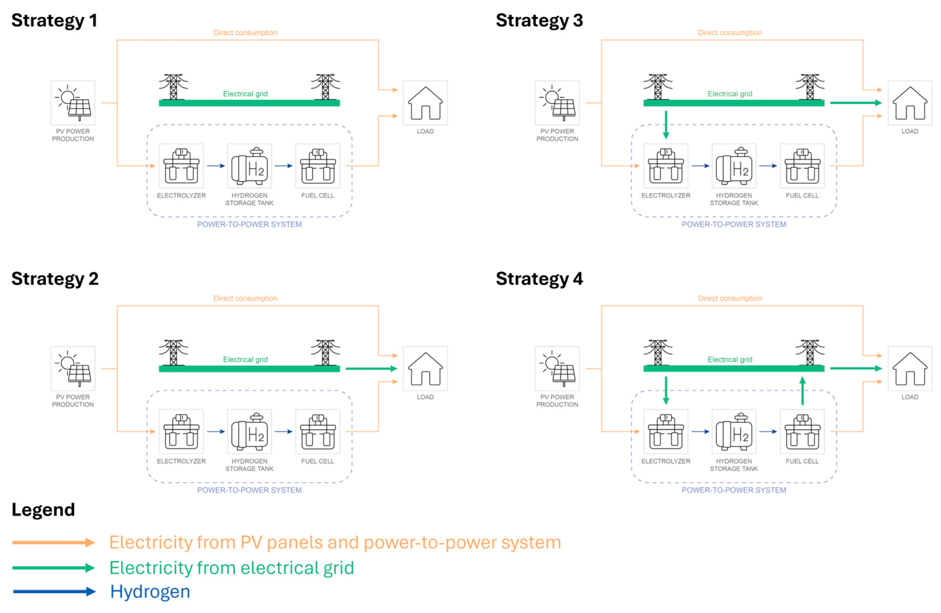
The four operating strategies (Figure 2) developed under these assumptions are presented in the following sub-chapters.

2.5.1. Strategy 1

The first strategy replicates a basic power-to-power system designed to meet the electricity demand exclusively through solar energy, without any connection to the electrical grid. When the PV generation exceeds the load, the surplus energy is directly used to operate the electrolyzer, producing hydrogen that is stored in a dedicated tank. Conversely, during periods of insufficient PV production, hydrogen is drawn from storage and converted back into electricity via the fuel cell to cover the deficit. A schematic representation of this configuration is provided in Figure 2 to facilitate an understanding of the system’s operation.

The design approach focuses on determining the optimal PV panel size required to fully meet the energy demand. Specifically, the PV production profile is scaled by a constant multiplier (k), thereby increasing the effective installed capacity and corresponding energy output. The system must ensure complete energy self-sufficiency, either by meeting demand directly from PV production or by storing excess energy for later use. A series of simulations were conducted using the full model described in the previous chapter. The methodology involves manually adjusting the k value and monitoring the hydrogen storage levels to avoid depletion or overfilling. For each value of k, the optimal solution is identified as the configuration in which the hydrogen mass at the end of each day matches the level recorded at the beginning of the week, ensuring system balance over the analysis period.

2.5.2. Strategy 2

This enhanced strategy builds upon the previous configuration by introducing the possibility of purchasing electricity from the grid to directly satisfy the power demand, thereby reducing reliance on the fuel cell. Under this scheme, the user’s energy needs can be met through three distinct pathways. First, when solar generation is sufficient, direct consumption is prioritized. If solar output is inadequate, the system can either draw electricity from the grid or activate the fuel cell to convert stored hydrogen—produced during periods of PV surplus—into electricity. A schematic representation of these operating modes is provided in Figure 2.

To determine the most cost-effective and operationally sustainable strategy, a price threshold is defined. This threshold represents the electricity price below which purchasing from the grid is economically favourable. When the market price exceeds this threshold, the system prioritizes the use of hydrogen via the fuel cell. This control parameter, referred to as Threshold 2, is calibrated to maintain a consistent hydrogen storage level over a daily cycle. By ensuring that the mass of hydrogen in the tank remains stable from day to day, the strategy prevents depletion and supports balanced energy management across the simulation period.

The value of Threshold 2 is not fixed a priori: during the simulation, it is swept from 25 to 105 EUR/MWh in 1 EUR/MWh increments.

For each candidate value, the model runs a one-week simulation, computes the total weekly cost, and selects the Threshold 2 that minimizes $C_{tot}$.

$$C_{tot}=C_{PV}+C_{ELY}+C_{FC}+C_{grid,buy}$$

(29)

By enforcing this cost-optimal set-point, a stable daily hydrogen inventory is maintained, avoiding both tank depletion and overfilling. This allows for a consistent evaluation of the resulting PV, electrolyzer and fuel cell costs. Since the optimization horizon is limited to one representative week, the total cost is expressed in EUR/week as the sum of all weekly contributions.

2.5.3. Strategy 3

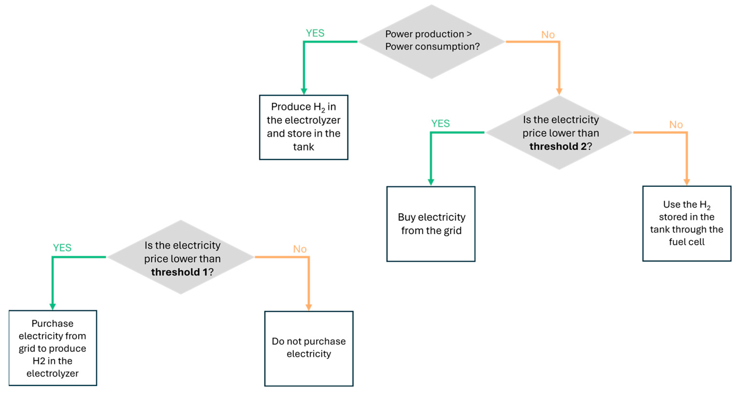
This strategy builds upon the previous one by introducing an additional feature: not only does it allow electricity purchases from the grid to meet energy demand—as in Strategy 2—but it also actively promotes electricity procurement specifically for hydrogen production via the electrolyzer, as illustrated in Figure 2. This approach takes advantage of periods with low electricity prices to increase hydrogen generation, which is subsequently stored and utilized by the fuel cell during high-price periods. In doing so, the system enhances overall efficiency and economic viability. Electricity purchases for hydrogen production are permitted only when the market price falls below a defined threshold.

From this point onward, Threshold 1 refers to the price limit below which electricity is purchased for hydrogen production, while Threshold 2 denotes the threshold below which electricity is directly used to meet the load demand (as in Strategy 2). The decision-making logic is depicted in the flowchart shown in Figure 3.

The methodology involves combining different combinations of Threshold 1 and Threshold 2 values.

Threshold 1 and Threshold 2 were first pre-selected by analyzing the hourly electricity prices, focusing on the most significant price fluctuations. These values reflect key points in the pricing trend, which should ensure cost-effective use of grid electricity for both load satisfaction and hydrogen production.

The optimization proceeds in three nested loops. First, a value of k is chosen to scale the nominal PV output, so that several possible array sizes can be assessed. For that specific k, we explore a grid of price limits: Threshold 1, which defines when cheap grid electricity is diverted to the electrolyzer, and Threshold 2, which defines when cheap grid electricity is taken directly to meet the load. Threshold 1 and Threshold 2 are varied independently from 25 to 100 EUR/MWh in 10 EUR/MWh increments. For every pair, the model runs a full-week simulation. During each run, it determines the extra grid energy required to keep the hydrogen storage quasi-steady, allocates this energy between hydrogen production and direct consumption according to the two thresholds and converts the result into a constant purchase power. The PV, electrolyzer and fuel cell sizes follow directly from the peak powers observed, and their annualized capital costs are added to the week-specific cost of the electricity purchased for hydrogen production and for load supply. The sum of these components yields the total weekly cost for that configuration. Keeping k fixed, Threshold 2 is then stepped through its entire range while Threshold 1 is held constant; once all Threshold 2 values have been evaluated, Threshold 1 is incremented and the process repeats. After the full grid has been scanned, the entire procedure is restarted with the next k value. The global optimum is simply the combination of k, Threshold 1 and Threshold 2 that produces the minimum total cost among all simulations.

$$C_{tot}=C_{PV}+C_{ELY}+C_{FC}+C_{grid,buy}$$

(30)

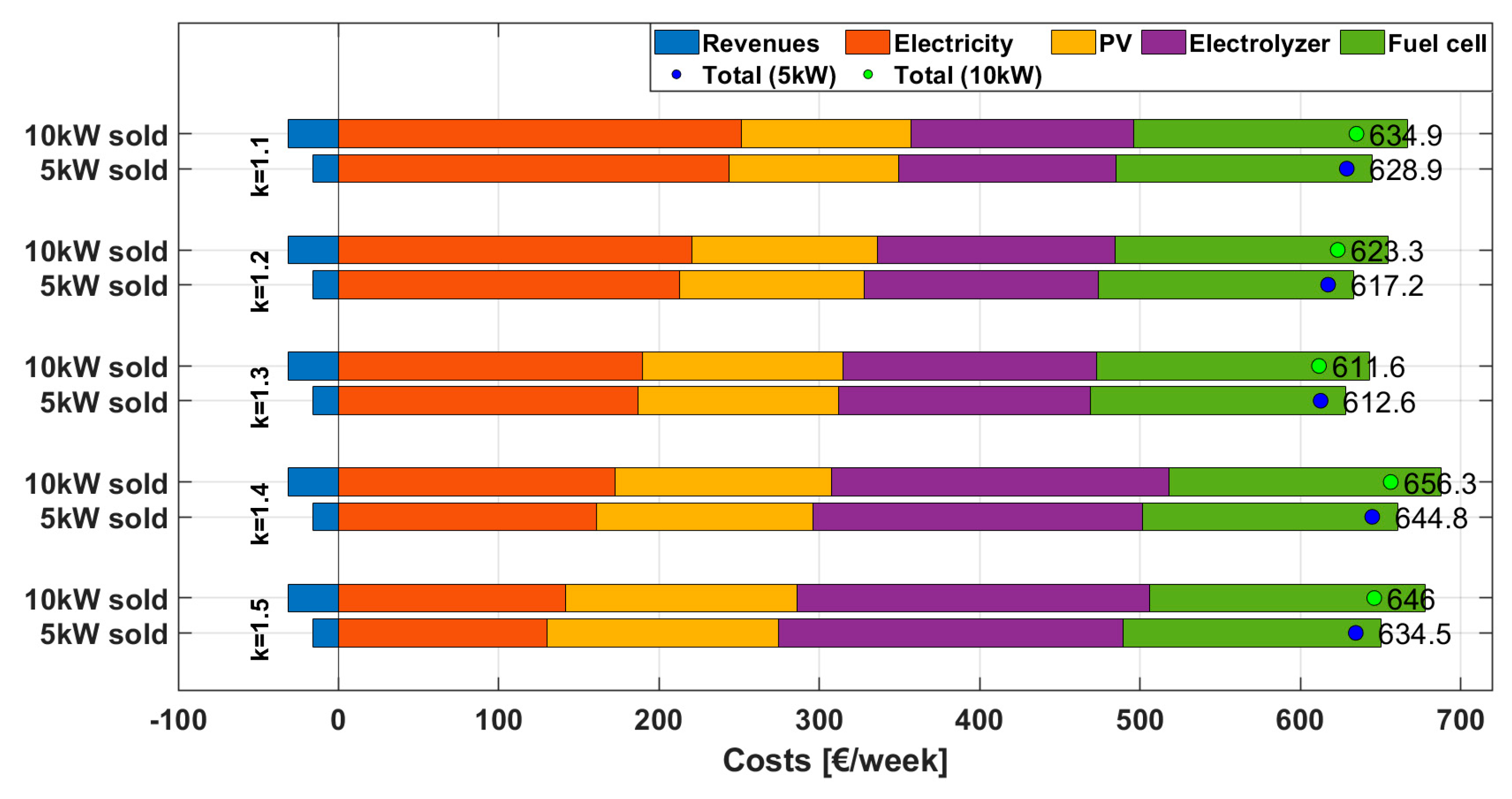
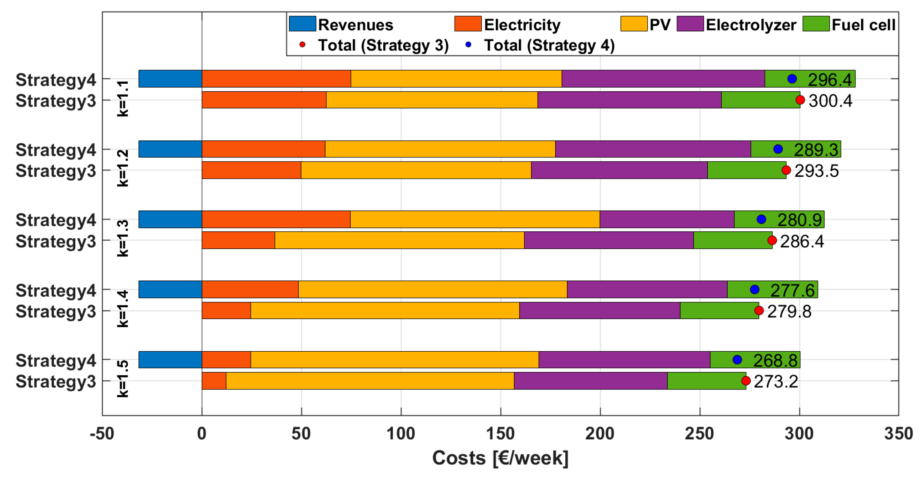
2.5.4. Strategy 4

A power-to-power system can serve not only for self-consumption purposes but also offers an attractive alternative opportunity for energy trading. Strategy 4 introduces this concept by enabling electricity purchases from the grid when prices are low and selling electricity back to the grid during high-price periods, thereby offering the potential for profit generation. The operational logic largely mirrors that of the previous strategy, using the same values for Threshold 1 and Threshold 2. However, as depicted in Figure 2, the key innovation in this strategy lies in the incorporation of bidirectional energy exchange, allowing the system to act as both a consumer and supplier of electricity, thereby optimizing both energy use and financial return based on market fluctuations. To maximize revenues, electricity export is scheduled during the period from 20:00 to 24:00, which is typically characterized by peak market prices. Two constant power levels—5 kW and 10 kW—are considered for each hour within this evening window. This configuration introduces variability in system performance and cost-effectiveness, depending on the selected power export level.

The methodology for purchasing electricity to generate hydrogen through the electrolyzer remains consistent with that used in Strategy 3 but now includes the additional energy required for export. As in previous strategies, the total energy to be purchased is divided by the number of hours when the electricity price is below Threshold 1 in order to determine the power input needed.

The electrolyzer size is then calculated based on the combined energy contributions from both PV surplus and electricity purchased from the grid. However, in contrast to earlier strategies, fuel cell sizing requires further consideration due to the added export requirement. Since peak electricity demand and export both occur during the night, when solar generation is unavailable, the fuel cell must be sized to cover both load demand and the fixed export power during the 20:00–24:00 period. As such, the fuel cell’s rated power is defined as the maximum of the net power deficit (demand minus PV contribution) plus the scheduled export power.

Finally, revenue from grid sales is calculated. For the sake of simplicity, the selling price is assumed to be equal to the purchasing price, although this assumption may differ in practical applications. This parity assumption represents an intentional upper-bound test: the most favourable feed-in tariff is adopted so that, if the export strategy proves uneconomic even under these conditions, any realistic reduction in the selling price can only further increase its cost disadvantage.

Finally, all cost components—including PV costs, fuel cell costs and revenues from electricity sales—are combined for various combinations of Threshold 1 and Threshold 2 to identify the configuration that minimizes the total cost for each selected size of the photovoltaic system. This holistic approach allows for optimizing the entire system, considering both the cost of purchased energy and the potential financial benefits of selling energy during low-demand periods, as shown in the following equation:

$$C_{tot}=C_{PV}+C_{ELY}+C_{FC}+C_{grid,buy}-R_{grid,sell}$$

(31)

Table 5. Variables and affected costs for each strategy.

Strategy	Variable	Definition	Cost Affected
Strategy 1	k *	PV size to completely meet the load	Cost of PV (↑)
Strategy 2	k	PV size	Cost of PV (↑), cost of electrolyzer (↑)
	Threshold 2 *	Amount of electricity purchased for direct consumption from the grid	Cost of electricity (↑), cost of electrolyzer (↓)
Strategy 3	k	PV size	Cost of PV (↑), cost of electrolyzer (↑)
	Threshold 2	Amount of electricity purchased for direct consumption from the grid	Cost of electricity (↑), cost of electrolyzer (↓)
	Threshold 1	Amount of electricity purchased for additional production of H2 in electrolyzer	Cost of electricity (↑), cost of electrolyzer (↑)
Strategy 4	k	PV size	Cost of PV (↑), cost of electrolyzer (↑)
	Threshold 2	Amount of electricity purchased for direct consumption from the grid	Cost of electricity (↑), cost of electrolyzer (↓)
	Threshold 1	Amount of electricity purchased for additional production of H2 in electrolyzer	Cost of electricity (↑), cost of electrolyzer (↑), revenues (↑)

Legend: ↑ An increase in the cost in relation to an increasing variable. ↓ A decrease in the cost in relation to an increasing variable. * Regulation parameter to stabilize the amount of hydrogen inside the tank. For Strategies 3 and 4, the regulation parameter is given by the amount of power bought from the electrical grid to produce H₂ to be used in the electrolyzer.

provides a summary of the key variables, their definitions and their relationships with system costs for each operating strategy. The table uses arrows to indicate how changes in each variable impact the overall cost.

3. Results

3.1. Strategy 1

Different trials have been carried out, and the optimal constant multiplier found is the one which multiplies the PV production by 2 (k = 2). In this way, the tank is never empty, and, at the same time, the mass of hydrogen is not increasing day by day.

However, this strategy cannot be considered a sustainable long-term solution because, being an off-grid system, the optimal PV size depends entirely on the specific energy production and demand profiles. If either of these input profiles—solar energy availability or energy demand—changes, the previously determined optimal PV size will no longer be valid, requiring recalibration. As a result, the system’s performance would fluctuate, making this approach highly sensitive to variations in weather conditions or load patterns and thus impractical for consistent operation.

3.2. Strategy 2

The second strategy introduces the option of purchasing electricity from the grid to meet energy demand directly, which becomes particularly advantageous when electricity prices are low.

The lowest total cost and associated component costs for each PV size are summarized in the Supplementary Materials. The configuration that finally allows reaching the lowest cost is the one using the k factor equal to 1.6. However, repeating the same process with different PV panel sizes results in weekly total costs that do not differ significantly from one another, as can be observed in Figure 4 (from 604 to 651 EUR/week). As a result, during the system design phase, this strategy will prioritize only the optimal threshold value based on the electricity cost profile. This approach simplifies decision-making by focusing on the most efficient operational balance rather than marginal cost differences between PV sizes.

3.3. Strategy 3

The third strategy introduces an additional feature: the option to purchase electricity specifically for hydrogen production via the electrolyzer. The best configuration for each size of PV selected is the one that minimizes the total cost, and details can be found in the Supplementary Materials. For each analyzed k value, the lowest costs are obtained when the highest value of Threshold 2 is selected (90 EUR/MWh for Strategies 4 and 5, 105 EUR/MWh for Strategies 1, 2 and 3). This finding is noteworthy, as it suggests that the most cost-effective configuration involves purchasing electricity over a longer period to directly meet the load demands, despite the associated higher electricity cost. However, this strategy allows for a minimal amount of energy to be purchased, which is then spread over a moderate number of hours, ensuring system stability. In fact, as Threshold 1 increases, the energy can be spread over more hours, reducing the required power. However, raising Threshold 1 does not necessarily lower costs, as electricity prices can become prohibitively high, depending on the threshold set.

In particular, the optimal value for Threshold 1 across all cases is 55 EUR/MWh, indicating that both the associated electricity costs and the cost of the electrolyzer are relatively low. Among the various k values analyzed, the lowest total cost is observed for k=1.2, with a weekly total cost of 611.20 EUR/week. The total costs for other PV sizes are shown in Figure 5. This outcome highlights the importance of balancing electricity purchases and system sizing to minimize overall costs while ensuring the operational efficiency of the power-to-power system.

3.4. Strategy 4

The optimal costs resulting from the analysis of Strategy 4 for each size of PV are summarized in the tables in the Supplementary Materials, distinguishing the amount of power sold.

The analysis reveals that the best results are achieved when using a Threshold 1 of 75 EUR/MWh. This threshold is optimal because it allows energy to be spread over several hours, reducing the required size of the electrolyzer. However, even though this configuration optimizes costs, it does not outperform Strategy 3 in terms of cost-effectiveness for any of the k values.

The most favourable configuration is with k = 1.3, both when 5 kW and 10 kW of power are sold (Figure 6). The total costs for these configurations are 612.58 EUR/week and 611.57 EUR/week, respectively, making them the most cost-efficient options in this strategy. The results suggest that the selling strategy is not more convenient than Strategy 3, since the final optimal cost is almost the same. It is important to recall that these figures already assume the most optimistic sell/buy price ratio (1.0). A more realistic reduction in the feed-in tariff would widen the cost gap in favour of Strategy 3, confirming that an export-oriented approach is not economically viable under present or foreseeable market conditions.

In addition, Strategy 4 results in higher utilization rates and duty cycles for both the electrolyzer and fuel cell due to the need to sustain export during non-solar hours. This increased operational stress may accelerate component degradation and further reduce the economic attractiveness of electricity selling under current cost assumptions.

All four control strategies rely on fixed values of Threshold 1 and Threshold 2 that are optimized based on a reference week. In reality, the economically optimal thresholds vary daily with the forecasted PV output, load profile and spot–price curve. By not adapting them in real time, the current model may over- or underestimate the value of arbitrage and hydrogen production, especially on days with atypical weather or price spikes. An obvious extension is to replace the static thresholds with an adaptive dispatcher (e.g., model-predictive control or a reinforcement-learning agent) that recalculates the buy/sell set-points each day (or hour) based on updated forecasts and system states. Such a controller could capture additional savings and reveal whether dynamic thresholding changes the ranking of the proposed strategies.

4. Discussion

Forecast Analysis

The findings from the preceding sections indicate that implementing a power-to-power system with the option to sell excess electricity is not economically favourable with these profiles of PV production, demand and electricity. As shown in the previous chapter, the lowest cost obtained from Strategy 3 is 611.20 EUR/week, compared to 611.57 EUR/week with 10 kW of power sold from Strategy 4. The revenue generated from selling the surplus electricity does not sufficiently cover the additional costs associated with upscaling the system components. Therefore, an alternative analysis has been conducted by considering variations in the costs, referring to 2050 forecasts of the electrolyzer and fuel cell. Figure 7 presents the comparison between Strategy 3 and Strategy 4 for each PV size coefficient. It is evident that, in the case of Strategy 3, the lowest cost is achieved when using a high PV size coefficient (k = 1.5). Despite the higher initial cost of the larger PV system, this choice results in reduced electricity purchases for both additional hydrogen production and direct load satisfaction. This cost-saving effect justifies the preference for a higher PV size coefficient in this optimization strategy.

Strategy 4 also includes electricity selling, relying on weekly patterns. The lowest costs obtained for each selected k value are noticeably lower with respect to Strategy 3. The optimal cost is again obtained with the same PV size coefficient (k = 1.5). As a consequence, it can be concluded that with the decrease in cost components, the selling strategy becomes more advantageous. Despite the need for larger electrolyzers and fuel cell sizes to cater to the production of additional electricity, the increased revenues generated from selling the surplus electricity outweigh the additional capital expenditure required for the larger components.

In other words, the selling strategy proves to be financially more feasible due to the overall reduction in costs. The higher initial investment in larger equipment is compensated by the greater income derived from selling the excess electricity. As a result, this approach becomes a more cost-effective and profitable solution, considering the cost forecast in 2050.

5. Conclusions

In this study, a comprehensive configuration of a hydrogen-based power-to-power system was developed and modelled using the Matlab/Simulink^® environment. The simulation aimed to assess the feasibility of implementing such a system within an energy community. The second phase of the research shifted focus towards the economic evaluation of various operational strategies. The first and simplest strategy involved meeting the energy demand solely through solar generation and the power-to-power system, with no reliance on electricity from the grid.

In contrast, the second strategy introduced the option of purchasing electricity from the grid when prices fell below a predefined threshold. This approach proved to be more practical than the previous one, as it ensured that energy demands were consistently met. Although it occasionally required purchasing electricity at higher prices during peak periods, the overall reliability of supply was enhanced, making this strategy more feasible for continuous load fulfillment.

The third strategy also included the possibility to purchase electricity specifically for the electrolyzer, enabling additional hydrogen production and storage for future use. This approach increased the system’s operational flexibility. The fourth and final strategy expanded the system’s functionality further by incorporating the ability to sell surplus electricity back to the grid, aiming to generate revenue.

In conclusion, when considering the round-trip efficiency of the power-to-power system and the associated equipment costs, the analysis indicates that electricity selling is not currently economically viable. The costs involved outweigh the potential revenue from selling excess electricity. However, with advancements in technology, reductions in equipment costs and improvements in system efficiency, electricity selling could become a financially attractive strategy in the future.

Future developments may explore the use of adaptive and forecast-based controllers to dynamically adjust the energy management strategy in response to daily or hourly variations in PV generation, electricity prices and demand profiles. This could improve the system’s responsiveness and further enhance its economic performance.