Abstract
The analysis and accurate identification of DC-side grounding faults in grid-connected photovoltaic (PV) inverters is a critical step in enhancing operation and maintenance capabilities and ensuring the safe operation of PV grid-connected systems. However, the characteristics of DC-side grounding faults remain unclear, and effective methods for identifying such faults are lacking. To address the need for leakage characteristic analysis and fault identification of DC-side grounding faults in grid-connected PV inverters, this paper first establishes an equivalent analysis model for DC-side grounding faults in three-phase grid-connected inverters. The formation mechanism and frequency-domain characteristics of residual current under DC-side fault conditions are analyzed, and the specific causes of different frequency components in the residual current are identified. Based on the leakage current mechanisms and statistical characteristics of grid-connected PV inverters, a multi-type DC-side grounding fault identification method is proposed using the light gradient-boosting machine (LGBM) algorithm. In the simulation case study, the proposed fault identification method, which combines mechanism characteristics and statistical characteristics, achieved an accuracy rate of 99%, which was significantly superior to traditional methods based solely on statistical characteristics and other machine learning algorithms. Real-time simulation verification shows that introducing mechanism-based features into grid-connected photovoltaic inverters can significantly improve the accuracy of identifying grounding faults on the DC side.
1. Introduction
Grid-connected photovoltaic (PV) power generation has become one of the primary methods of energy supply [1,2]. As the core component of PV systems, the performance of grid-connected inverters directly impacts the reliability and efficiency of the entire system [3]. Compared to traditional isolated inverters, non-isolated grid-connected PV inverters have gained significant attention and application in the market due to their advantages of compact size, lower cost, and higher efficiency [4]. However, a notable drawback of non-isolated inverters is the absence of transformer isolation, which leads to high-frequency common-mode voltage variations that induce leakage current issues, resulting in DC-side grounding faults [5]. Additionally, various factors, such as insulation damage, environmental conditions, and temperature fluctuations, contribute to the diversity of DC-side grounding faults, increasing potential safety hazards, including risks of electric shock and equipment damage. According to the VDE-0126-1-1 standard [6], PV systems must disconnect from the grid when the leakage current exceeds 300 mA. Similarly, technical specifications for grid-connected PV inverters [7] require inverters with a rated output not exceeding 30 kVA to disconnect within 0.3 s and issue a fault signal if the residual current continuously exceeds 300 mA. Thus, for non-isolated grid-connected inverters, accurately identifying DC-side grounding faults is critical to improving system safety and reliability.
Based on fault occurrence locations, PV inverter faults can be categorized into three main types: DC-side faults, AC-side faults, and inverter body faults. DC-side faults include overvoltage, undervoltage, and grounding faults, while AC-side faults encompass overvoltage, overcurrent, and frequency abnormalities. Inverter body faults include power switch failures, module overheating, and sensor malfunctions [8,9]. At present, the methods for diagnosing inverter faults are relatively mature. However, the types of fault detection are rather concentrated, mostly targeting open-circuit and short-circuit faults of passive components in photovoltaic inverters, faults of the AC power grid connected to the inverters, and faults of power switches in inverters [10,11,12,13]. For example, ref. [14] discusses commutation failures caused by AC faults on the rectifier side and proposes a fault diagnosis method that combines wavelet transform and wavelet neural networks. The authors of [15] identify power electronic switch faults under open-circuit and low-level conditions for a cascaded H-bridge five-level inverter using a high-performance diagnostic system. However, research on DC-side grounding faults is primarily concentrated on suppressing and detecting common-mode currents induced by parasitic capacitance grounding on the DC side [16]. While these studies explore various fault diagnosis methods, identifying DC-side grounding faults is crucial for efficient PV inverter operation and maintenance. This study aims to investigate DC-side grounding fault identification methods to achieve accurate fault classification and improve fault-handling efficiency in PV systems.
Extensive research has been conducted on fault diagnostic feature selection for non-isolated grid-connected PV inverters. Early studies focused on parameters such as voltage, current amplitude, frequency, and phase [17,18,19]. Subsequently, statistical features such as the mean, root mean square, peak value, slope, and kurtosis of these signals were used for fault diagnosis [20]. Such methods are simple to calculate and do not require complex hardware. However, the problem of feature overlap (such as the similarity of statistical features for different faults) leads to low diagnostic accuracy and sensitivity to noise. Although simple and intuitive, these methods often suffer from feature overlap, leading to low accuracy. Some references [21,22] have proposed non-invasive fault diagnosis methods using electromagnetic characteristics and common-mode signals from the DC bus. However, these methods are limited to power device faults and do not provide comprehensive fault diagnosis for PV inverters. To ensure the accuracy of DC-side grounding fault identification, it is necessary to fully explore the differences in residual current mechanism-based features under various fault conditions.
The development of inverter fault diagnosis methods has been quite rapid. Currently, fault detection methods based on artificial intelligence (AI) have high accuracy and strong generalization ability and are important tools for fault diagnosis in inverter systems [23]. Typical AI algorithms used in fault monitoring include support vector machines (SVMs), random forest (RF), convolutional neural networks (CNNs), recurrent neural networks (RNNs), gradient-boosting decision trees (GBDTs), and extreme gradient boosting (XGBoost) [14,24,25,26]. Among these, the light gradient-boosting machine (LGBM) has demonstrated significant advantages in classification and regression tasks, including support for sparse data, built-in regularization to avoid overfitting, efficient parallel processing, and robustness to missing values. The authors of [27] applied an LGBM to diagnose the faults of belt conveyors, achieving the accurate identification of faults in coal production processes. In addition, ref. [28] developed an LGBM-based fault diagnosis model for high-dimensional fault features in analog circuits, demonstrating superior fault diagnosis accuracy compared to CNN, RNN, and GBDT models. Regarding the grounding faults on the DC side of inverters, there has been no systematic analysis of the differences in the mechanism characteristics of residual current. Moreover, traditional AI models face difficulties in balancing the requirements of real-time performance and accuracy. This paper combines the lightweight advantages of an LGBM and the fusion of multi-physical quantity features to fill this gap.
This paper is structured as follows: Section 1 introduces the research background and significance. Section 2 constructs an equivalent model for the grounding fault on the DC side of the grid-connected inverter. Section 3 analyzes the specific causes of leakage current generation and verifies the results. Section 4 conducts a mechanism analysis of the leakage current characteristics under the grounding fault on the DC side. Section 5 proposes an LGBM-based method for leakage fault classification, effectively addressing the challenge of DC-side fault identification through the fusion of mechanistic and statistical features. Section 6 conducts comprehensive testing on the proposed method using a test dataset, demonstrating its effectiveness and high accuracy. Section 7 verifies the effectiveness and accuracy of the DC-side grounding fault discrimination method proposed in this paper through real-time simulation. Section 8 presents the conclusions and future research directions.
2. Equivalent Model of DC-Side Grounding Faults in Grid-Connected Inverters
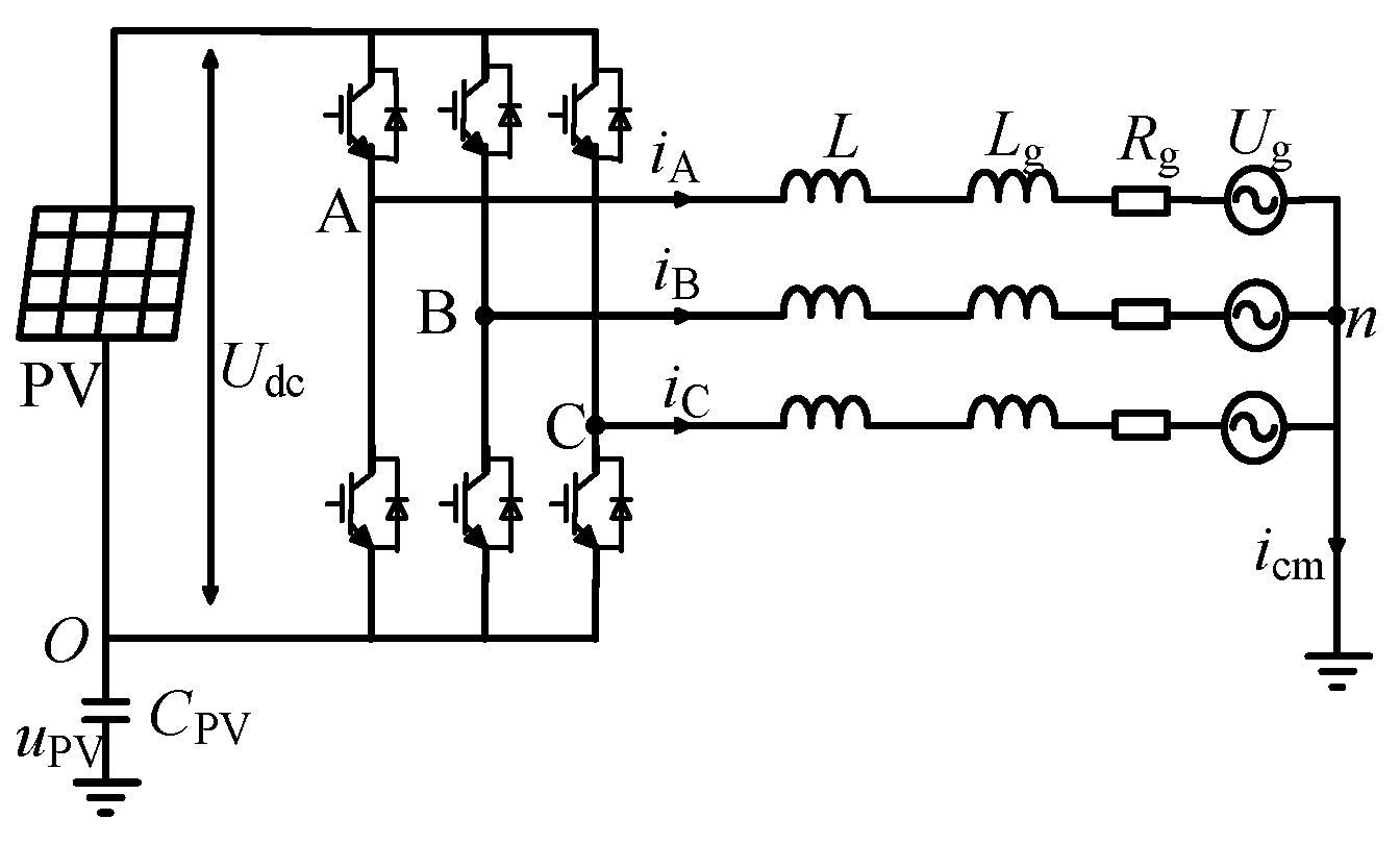
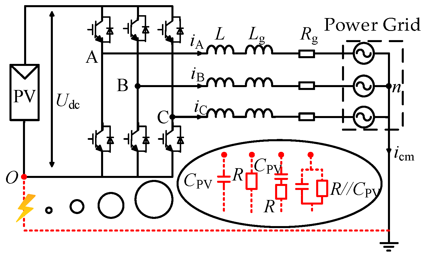
The structure of a non-isolated three-phase grid-connected photovoltaic (PV) inverter is shown in Figure 1. Due to environmental factors, the parasitic capacitance Cpv between the PV panels and the ground inherently exists, where upv represents the voltage across the parasitic capacitance. In the L-type filter, L denotes the three-phase filter inductance, Lg represents the grid-side inductance, Rg represents the grid-side resistance, and Ug is the grid voltage. O refers to the negative terminal of the DC side. The current icm, flowing from n to the ground, is the common-mode current. Udc is the equivalent input voltage of the PV panels.

Figure 1.
Non-isolated three-phase PV grid-connected inverter.
The three-phase circuit equations based on Kirchhoff’s Voltage Law (KVL) are established as follows:
In these equations, UJO represents the output voltage of the J-phase bridge arm; iJ denotes the current of the J-phase bridge arm; ej is the grid voltage of phase J; J = A,B,C; and j = a,b,c. Considering the grid as a three-phase symmetrical system, Equation (1) can be simplified as follows:
The expression for the common-mode current icm can be derived as follows:
In this equation, upv represents the average voltage across the parasitic capacitance of the bus. From Equation (3), the following can be derived:
The expression for the voltage difference unO between the grid neutral point n and the DC-side negative terminal O is given as:
Substituting Equations (3) to (5) into Equation (2) yields the following:
Taking point O as the reference node, the voltages at points A, B, and C relative to point O are denoted as UAO, UBO, and UCO, respectively. In a three-phase non-isolated photovoltaic grid-connected system, the formulas for common-mode voltage UCM and differential-mode voltage UDM are as follows:
Under the condition LA = LB = LC = L, the total common-mode voltage can be expressed as:
Substituting Equation (9) into Equation (6), the total excitation ucm of the leakage circuit is obtained as [29]:
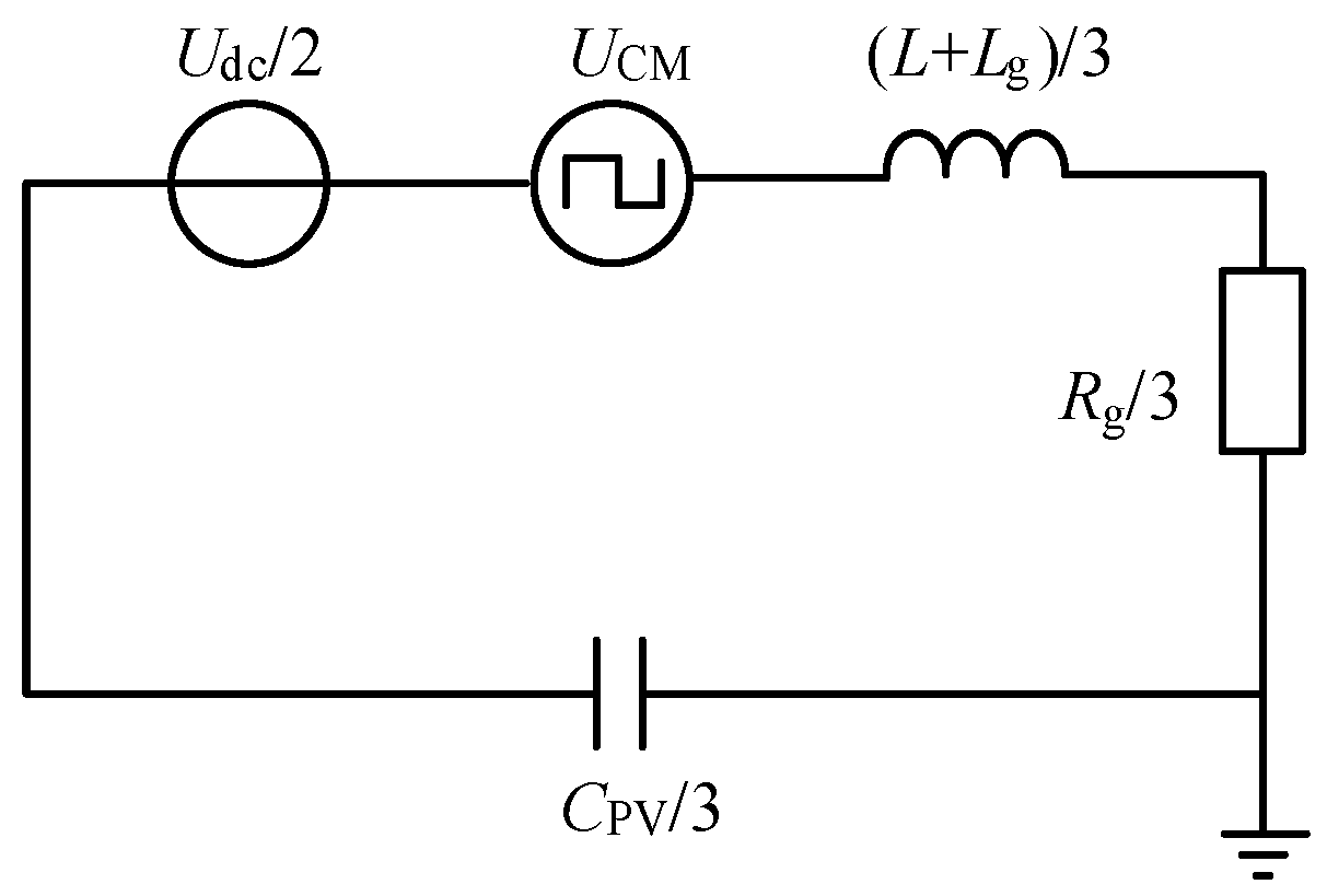
From Equation (10), the leakage equivalent model of the non-isolated three-phase grid-connected photovoltaic inverter can be derived, as shown in Figure 2.
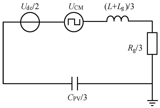
Figure 2.
Equivalent model of DC-side grounding faults in grid-connected inverters.
As shown in Figure 2, the equivalent model of DC-side grounding faults in non-isolated three-phase grid-connected photovoltaic inverters includes two excitation sources:
- DC voltage of 0.5Udc:
This voltage is determined by the operating principle of the bridge inverter and the characteristics of PWM control. The voltage at the negative terminal of the inverter’s DC side, relative to the neutral point, measures half of the DC source voltage.
- Common-mode voltage (UCM):
This voltage is determined by the output voltages UAO, UBO, and UCO of each bridge arm. Investigating the modulation effect and dead-time effect of the three-phase inverter and analyzing the voltage spectrum characteristics generated by these effects are critical steps in understanding the causes of residual current components under different conditions.
3. Formation Mechanism of the Wide-Band Residual Current in Grid-Connected Inverters
3.1. The Cause of the Generation of the DC Component
The voltage at the negative terminal of the inverter’s DC side, measured relative to the neutral point, equals half of the DC source voltage. This phenomenon arises primarily from the grounding configuration of the DC source and the principles of voltage distribution. In typical inverter designs, the negative terminal of the DC source (such as a battery or photovoltaic panels) is often grounded and used as a reference point, i.e., the neutral point. As a result, the total voltage between the positive and negative terminals of the DC source is Udc, with the negative terminal relative to the neutral point being −Udc/2 and the positive terminal being Udc/2. This symmetrical voltage distribution is a direct outcome of the grounded reference point and the symmetry of the DC source voltage [30].
The symmetrical voltage configuration helps reduce electromagnetic interference (EMI) since symmetric voltage waveforms can minimize electromagnetic noise, thereby improving the inverter’s efficiency and reliability. Additionally, the symmetric power configuration effectively balances current loads, preventing load imbalances caused by extreme voltage levels at a single terminal. This contributes to load distribution and enhances the system’s long-term reliability. Therefore, the voltage at the negative terminal of the DC side, being half of the DC source voltage relative to the neutral point, is a direct result of the symmetric power configuration.
3.2. The Cause of the Generation of the Low-Frequency Component
An ideal photovoltaic inverter’s output voltage contains almost no low-order harmonics, with harmonics primarily related to the carrier frequency. However, the existence of a dead time introduces a series of low-frequency harmonic voltage components. When considering the dead-time effect, the low-frequency harmonic voltage of phase A in a three-phase inverter can be expressed as:
In this equation, ω0 = 2πf0, where f0 represents the fundamental frequency, Udc is the DC-side voltage, N1 is the carrier ratio, td is the dead-time delay, and φA is the initial phase of phase A.
From Equation (11), it can be observed that the amplitude of each harmonic is proportional to f0 or td. As f0 or td increases, the amplitude of the harmonic components in the output voltage also increases proportionally. In the actual output voltage waveform of a PWM inverter, odd-order harmonics also exist, distorting the output voltage waveform.
Since the phase voltages of phases A, B, and C in the inverter are phase-shifted by 2π/3 relative to each other, the low-frequency harmonic voltage expressions for phases B and C can be similarly derived. For harmonics with a frequency of 3nf0 (where n is an integer), the initial phases of phases φB and φC, denoted as φA − 2π/3 and φA + 2π/3, respectively, cause the harmonics at 3nf0 in phases B and C to have the same phase as those in phase A. This phase alignment generates a zero-sequence voltage, which in turn forms a zero-sequence current. The harmonic orders of the zero-sequence voltage are odd multiples of three, with frequencies such as 3f0, 9f0,…, (6n − 3)f0. Therefore, the dead-time effect of the inverter generates a zero-sequence leakage current at frequencies of 3f0, 9f0,…, (6n − 3)f0. Due to the rapid attenuation of high-frequency components, this type of leakage current is primarily composed of low-frequency components in the frequency spectrum.
3.3. The Cause of the Generation of the High-Frequency Component
Due to the modulation effect of the three-phase inverter, voltage components corresponding to switching harmonics are generated. Taking bipolar modulation as an example, the high-frequency voltage harmonics of phase A in the three-phase inverter can be expressed as:
In this equation, ωs = 2πfs, where fs is the carrier frequency; Udc is the DC supply voltage; M is the modulation index; N is the carrier ratio; m is the harmonic order relative to the carrier; n is the harmonic order relative to the modulation wave; φ is the initial phase of the modulation wave; and J0 and Jn are the first-kind Bessel functions.
Since the phase voltages of phases A, B, and C in the three-phase inverter are phase-shifted by 2π/3, the high-frequency voltage harmonic expressions for phases B and C can also be derived. In the expression, the first term corresponds to the m-th harmonic of the carrier, while the second term represents the upper and lower sideband harmonics of the m-th carrier harmonic.
For the m-th carrier harmonic in the first term, it is important to note that the voltage components of the odd-order carrier harmonics generated by phases A, B, and C do not contain the initial phase. Consequently, the phase components of the voltages in phases A, B, and C are identical, resulting in a certain amount of zero-sequence voltage and, therefore, zero-sequence current. The harmonic order of this current corresponds to odd multiples of the carrier frequency, i.e., odd-order switching harmonics. Since the switching frequency is typically in the kilohertz range, the leakage current manifests as a high-frequency zero-sequence leakage current at odd multiples of the switching frequency. Specifically, the switching effect of the inverter generates a high-frequency zero-sequence leakage current with frequencies of fs, 3fs,…, (2n − 1)fs, where fs is the switching frequency.
3.4. Model Validation
To validate the specific causes of residual current generation in the aforementioned non-isolated three-phase grid-connected photovoltaic inverter, the three excitation sources in the leakage equivalent model were tested. A leakage equivalent validation model for the non-isolated three-phase grid-connected photovoltaic inverter was constructed, as shown in Figure 3.
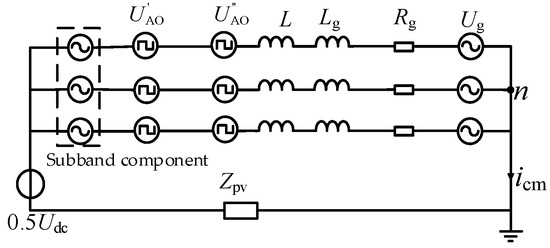
Figure 3.
Leakage equivalent verification model of a non-isolated three-phase PV grid-connected inverter.
Residual current validation was conducted based on the inverter equivalent validation model shown in Figure 3, using the equivalent parameters listed in Table 1. Among these, 0.5Udc represents the equivalent voltage source equal to half of the DC source voltage, U’AO corresponds to the equivalent harmonic voltage source generated by the inverter’s dead-time effect, and U″AO represents the equivalent harmonic voltage source generated by the inverter’s switching effect.

Table 1.
Parameters of the leakage current verification simulation model.
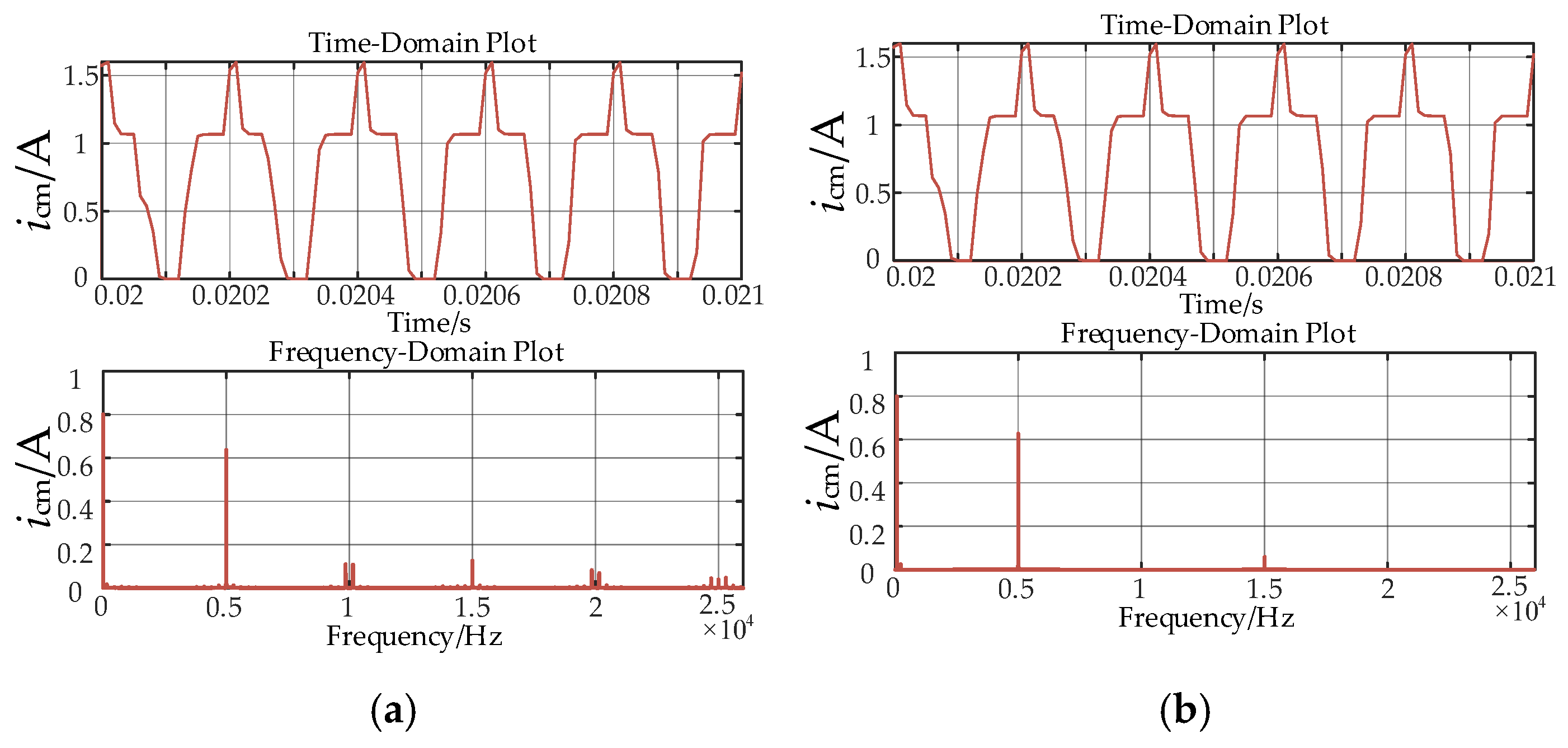
The detailed simulation model and the equivalent model’s resistive fault residual current FFT analysis comparison results are shown in Figure 4 and Table 2.
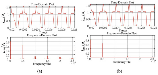
Figure 4.
Time-domain and frequency-domain curve diagrams. (a) The residual current of the simulation model; (b) the residual current of the equivalent model.
Table 2.
Amplitude and phase of residual current verification.
Figure 4a represents the FFT harmonic component analysis of the residual current before the equivalent voltage sources, while Figure 4b shows the FFT harmonic component analysis after the equivalent voltage sources. FAs can be seen from Figure 4a, where the leakage current mainly consists of DC components, odd multiples of the switching frequency high-frequency components, and odd multiples of the fundamental frequency low-frequency components. Comparing Figure 4b with Figure 4a, it is evident that the equivalent model closely reproduces the spectral components of the residual current, as observed in the actual simulation results. Notably, the differences in amplitude for each frequency component between the simulation and the model are minimal, demonstrating the high accuracy of the equivalent model.
Table 2 provides a detailed comparison of the amplitudes and phases of the main components between the simulation results and the equivalent circuit calculation results. From Table 2, it can be observed that the differences in amplitude and phase between the actual simulation and the equivalent model are minimal. This indicates that the model accurately reproduces the simulation results, demonstrating that the equivalent model effectively validates the residual current mechanism features investigated in this study.
Table 2 provides a detailed comparison of the amplitude and phase of major components between simulation results and equivalent circuit calculations. From Table 2, it can be observed through amplitude and phase comparison that the differences in amplitude and phase between actual simulations and the equivalent model are very small. The model accurately reproduces the simulation results, confirming the validity of the equivalent model in investigating the mechanism characteristics of the leakage current. According to the simulation data, it is evident that the low-frequency zero-sequence leakage current caused by the dead-time effect is relatively small and can be neglected. The high-frequency zero-sequence voltage generated by the switching effect has a relatively large residual current, which is the main factor causing leakage current. Moreover, the leakage current mainly consists of the DC component leakage current and the zero-sequence leakage current under the switching frequency harmonics. Therefore, based on the current characteristics of the DC component of the residual current and the high-frequency component under the switching frequency harmonics, different fault discrimination methods for leakage circuits can be studied.
4. Leakage Characteristics Analysis Under DC-Side Grounding Faults in Grid-Connected Inverters
Due to factors such as the parasitic capacitance of PV panels to the ground and insulation damage, the grounding impedance in the inverter’s DC-side leakage circuit may exhibit various configurations, including resistance, capacitance, or combinations of both in series or in parallel. These configurations lead to multiple fault scenarios, such as pure resistive leakage faults, pure capacitive leakage faults, resistive–capacitive series leakage faults, and resistive–capacitive parallel leakage faults.
This study takes these four typical fault types as examples to analyze their leakage characteristics. The structure of the non-isolated three-phase grid-connected photovoltaic inverter under different fault types is shown in Figure 5.

Figure 5.
Non-isolated three-phase PV grid-connected inverter under different fault types.
The red dotted line in the figure represents the short-circuit path on the DC side of the inverter, and the lightning symbol indicates that a short-circuit fault has occurred. The circuit parameters are consistent with those in Table 1, with a grounding resistance of 500 Ω and a grounding capacitance of 1 μF. Based on the models of the non-isolated three-phase grid-connected photovoltaic inverter under different fault types, constructed as shown in Figure 5, the current signal icm was analyzed for its spectral distribution, phase characteristics, and wavelet features under the fault scenarios. The results are illustrated in Figure 6, Figure 7, Figure 8 and Figure 9.

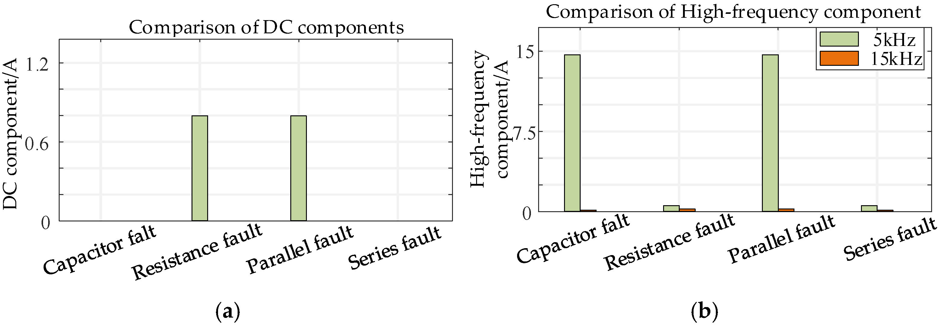
Figure 6.
Comparison of harmonic components under different fault types. (a) DC component comparison diagram; (b) high-frequency component comparison diagram.

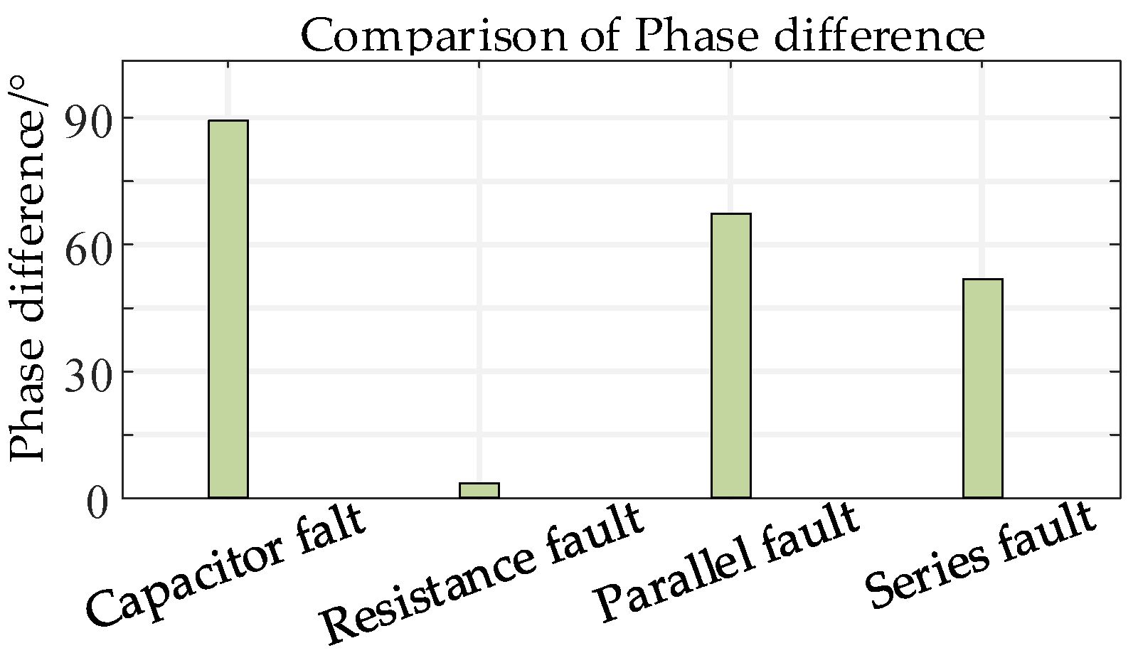
Figure 7.
Phase difference between the leakage current and voltage unO under different fault types.
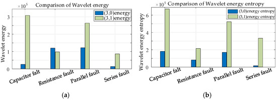
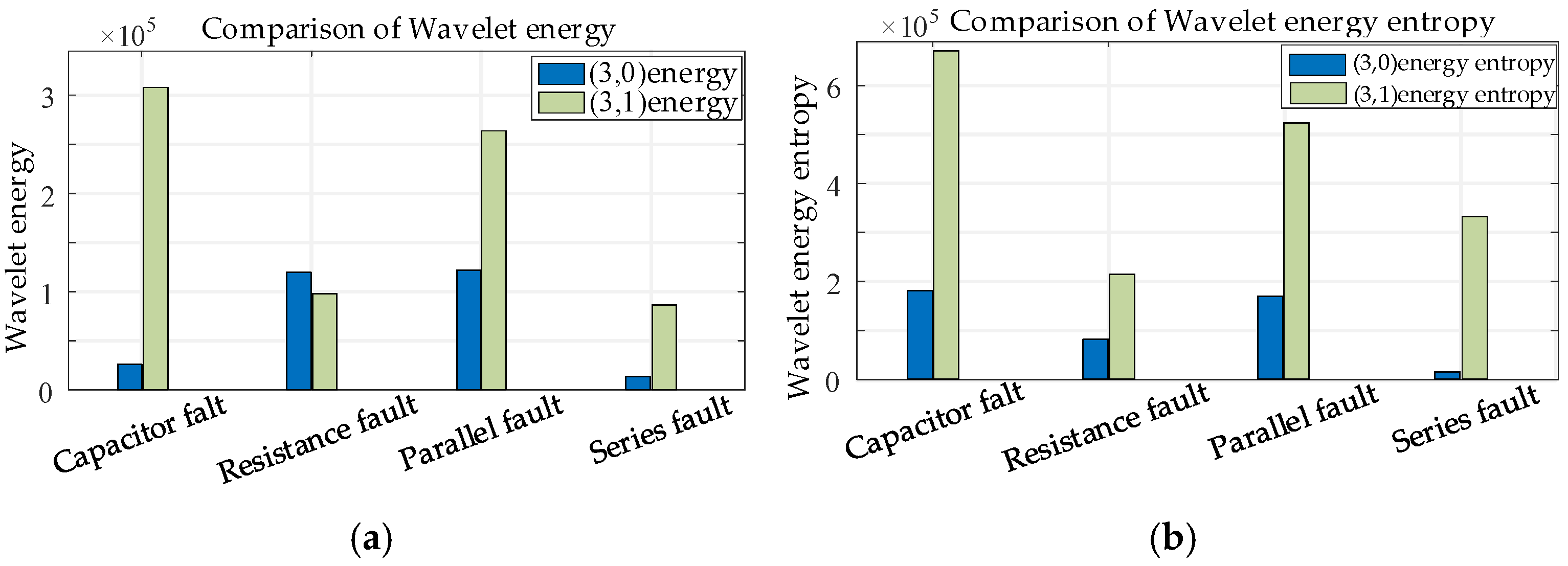
Figure 8.
Comparison of wavelet features under different fault types. (a) Wavelet energy comparison diagram; (b) wavelet energy entropy comparison diagram.
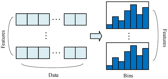
Figure 9.
Histogram algorithm schematic.
It can be observed that these features vary significantly under different fault conditions. Therefore, the above three types of features can be utilized to identify and distinguish the types of DC-side leakage faults in the inverter. The following provides an analysis of the leakage characteristics for the four fault types:
① Different fault types exhibit varying sensitivities to frequency characteristics. By analyzing these frequency components, specific types of faults can be identified. The harmonic components of the four different fault types, as derived from the FFT results, are shown in Figure 6.
Figure 6a illustrates the DC components for the four fault types. Among these, since no capacitor is directly connected in series within the leakage circuit, pure resistive faults and resistive–capacitive parallel faults result in more significant DC components during leakage.
Figure 6b depicts the harmonic components at specific frequencies for the four fault types. As shown in Table 2 and Figure 6b, the residual current components are primarily concentrated at 5 kHz and 15 kHz, corresponding to odd multiples of the switching frequency. It can be observed that pure capacitive faults and resistive–capacitive parallel faults generate higher values of high-frequency residual currents, which are the primary contributors to the residual current components.
② Phase variations are closely related to changes in impedance. Different faults (e.g., pure capacitive faults or pure resistive faults) result in varying degrees of phase shifts in the signal. The phase differences between the residual current icm and the voltage unO under the DC component for the four fault types are extracted, and the results are shown in Figure 7.
Figure 7 shows the phase differences between the residual current and the voltage unO for the four fault types. As observed in Figure 7, the phase difference between the residual current and unO is minimal, approximately 0, under pure resistive faults. In contrast, for resistive–capacitive parallel faults, the phase difference between the residual current and unO is significantly larger.
③ Wavelet analysis can decompose a signal into different frequency bands, enabling the analysis of energy distribution within each band to detect anomalies in specific bands. By analyzing wavelet entropy, changes in circuit complexity under different fault conditions can be revealed, aiding in more precise classification.
In this study, the db40 wavelet and Shannon entropy were selected as the optimal wavelet packet basis for extracting and decomposing the residual current data of the inverter leakage circuit. The original residual current signal icm (sampling frequency of 50,000 Hz) was subjected to a three-level wavelet packet decomposition. After the three-level decomposition, the frequency band was divided into eight regions, each with a bandwidth of 3125 Hz. Considering the disordered frequency band sequence problem in wavelet packet decomposition, the frequency range and harmonic components corresponding to the wavelet packet decomposition nodes (3,0) to (3,7) are shown in Table 3.
Table 3.
Frequency band division of wavelet packet decomposition.
Based on the wavelet packet transformation, the energy and Shannon entropy of different nodes under the four fault types can be obtained, as shown in Figure 8.
Figure 8a shows the energy comparison for the four fault types. According to Table 3, node (3,0) contains the DC component, and node (3,1) contains the harmonic components at the switching frequency. These are the primary components of the residual current. Thus, these two nodes are selected as references. From Figure 8a, it can be observed that by examining the distribution of “Energy31” and “Energy30”, certain faults exhibit stronger energy in specific frequency bands. This frequency band characteristic is highly effective for distinguishing between parallel and series faults.
Figure 8b presents the wavelet entropy comparison for the four fault types. The figure reveals that certain faults have significantly higher entropy values, indicating that the signal is more complex or random under these fault conditions. By analyzing changes in entropy, normal signals can be effectively distinguished from fault signals. Differences in energy values reflect the concentration of the signal in specific frequency bands, while entropy provides information about the complexity of the signal within those bands. This combination of characteristics helps us to more clearly differentiate between various fault types.
5. LGBM-Based Identification Method for DC-Side Grounding Faults in Inverters
5.1. Principle of the LGBM Algorithm
The light gradient-boosting machine (LightGBM), introduced by Microsoft in 2017, is an ensemble algorithm that uses decision trees as base classifiers. It leverages the histogram-based algorithm to overcome the limitations of traditional gradient-boosting decision tree (GBDT) methods, such as slow training speeds and susceptibility to overfitting. As a result, LightGBM has been widely applied in fields such as classification, regression, and feature importance ranking.
Leakage fault classification involves a variety of complex features with nonlinear relationships, and the distribution of different fault types (e.g., parasitic resistance and parasitic capacitance) may be imbalanced. LightGBM employs ensemble learning to approximate the objective function effectively through multiple iterations of learners. It not only captures the nonlinear relationships among features but also efficiently handles high-dimensional and sparse features using its histogram algorithm, significantly improving training efficiency and memory utilization. Furthermore, LightGBM’s unique leaf-wise growth strategy prioritizes splitting the node with the largest gain, enhancing the model’s classification capability and sensitivity to minority classes. Given the high accuracy and efficiency requirements for leakage fault classification, LightGBM can avoid overfitting through hyperparameter tuning (e.g., tree depth, learning rate, and number of trees) and early stopping mechanisms, ensuring the stability and accuracy of the classification model.
Thus, in leakage fault classification tasks, LightGBM proves to be an efficient and reliable classification method due to its exceptional performance and robust feature handling capabilities.
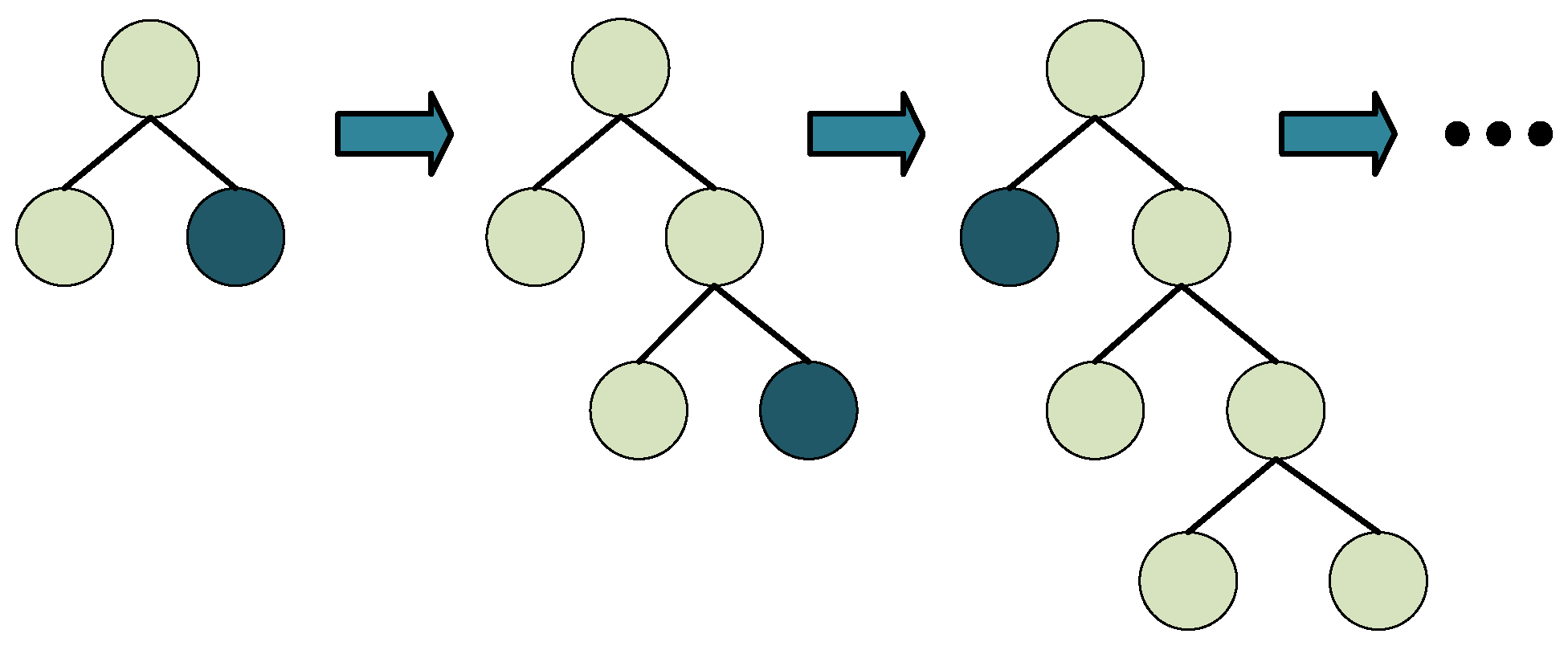
Figure 9 intuitively illustrates the histogram-based algorithm principle of LightGBM in leakage fault classification. The histogram algorithm adopts a discretization process, converting continuous floating-point feature values into k integers and constructing a histogram with a width of k. For the input continuous leakage feature data, LightGBM first discretizes the data into a fixed number of intervals (bins). By analyzing the feature distribution within each interval, it quickly computes the split gain to identify the optimal split point, optimizing the decision tree’s node division.
Figure 10 illustrates the principle of the leaf-wise tree growth strategy in LightGBM. In leakage fault classification, LightGBM prioritizes splitting the leaf node with the highest current gain, rather than splitting nodes evenly by levels (level-wise). For leakage feature data, this strategy enables the model to quickly capture key features associated with fault types, improving the classification capability while avoiding unnecessary splits. This approach maintains model efficiency and generalization by minimizing the value of the loss function and ensuring the tree depth does not exceed a predefined limit.

Figure 10.
Leaf-wise tree growth schematic.
The leaf-wise strategy is particularly suitable for handling the nonlinear relationships among complex features, ensuring the efficiency and accuracy of fault classification.
5.2. Fault Feature Selection
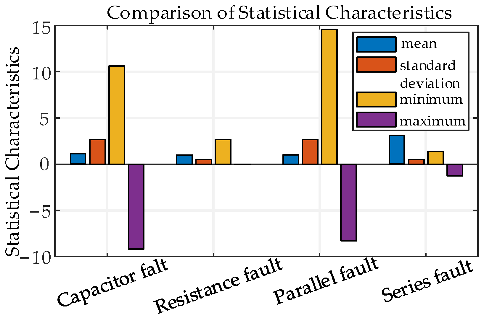
Traditional fault model classification primarily uses statistical features as input features. The mean, standard deviation, maximum, and minimum are fundamental statistical features of a signal, effectively describing its overall trend and variability. These features are simple to compute and do not require complex processing steps, making them highly suitable as basic features for fault diagnosis.
These features can quickly capture the fundamental changes in the signal, providing an intuitive basis for subsequent fault classification. A comparison of the basic statistical features for the four fault types is shown in Figure 11.
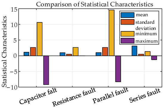
Figure 11.
Comparison of basic statistical features under different fault types.
From Figure 11, it can be observed that different fault types exhibit significant differences in mean, standard deviation, maximum, and minimum values. These differences provide valuable support for fault classification. Based on the leakage mechanism features of inverters explored in Section 3, the following conclusions can be drawn:
- The magnitude and presence of the DC component are strongly associated with different fault types, making it an effective criterion for fault type identification;
- The magnitude of high-frequency harmonic components at the switching frequency is also strongly correlated with fault types;
- The comparison of phase differences reveals the impact of these faults on circuit phase characteristics, helping to identify fault types;
- The energy and entropy extracted through wavelet analysis exhibit stable differences among different fault types, enhancing the accuracy of fault discrimination and enabling the model to more clearly distinguish between fault types.
In summary, the above mechanism-based and statistical features of the current signal are used as input variables for model training. The specific feature variables selected are listed in Table 4.
Table 4.
Parameter description for feature selection.
In Table 4, x1–x8 represent the signal mechanism features investigated in this study, while x9–x12 are the basic signal features typically used in classification models. y1–y4 correspond to the four different fault types.
5.3. LGBM Hyperparameter Optimization
Bayesian optimization is an essential technique for improving the performance of the LGBM model, especially when dealing with a complex hyperparameter space. Since the performance of the LGBM model largely depends on the choice of hyperparameters, Bayesian optimization intelligently searches the hyperparameter space, allowing for the identification of the optimal hyperparameter combination with fewer evaluations. This approach avoids the inefficiency and high computational cost of traditional grid searches while mitigating overfitting and underfitting, thus enhancing the model’s accuracy and generalization capability.
Bayesian optimization offers significant advantages in tuning LGBM models, making it an effective tool for boosting model performance. The hyperparameters of the LGBM model can be categorized into four main groups: parameters that affect the structure and learning of decision trees, parameters that influence training speed, parameters that improve accuracy, and parameters that prevent overfitting. Based on the impact of different hyperparameters on the model and the desired optimization direction, the search ranges for the parameters are defined. The meanings and optimization ranges for each parameter are listed in Table 5.
Table 5.
Hyperparameter optimization range for the LGBM model.
5.4. Grounding Fault Identification Process for Grid-Connected Inverters
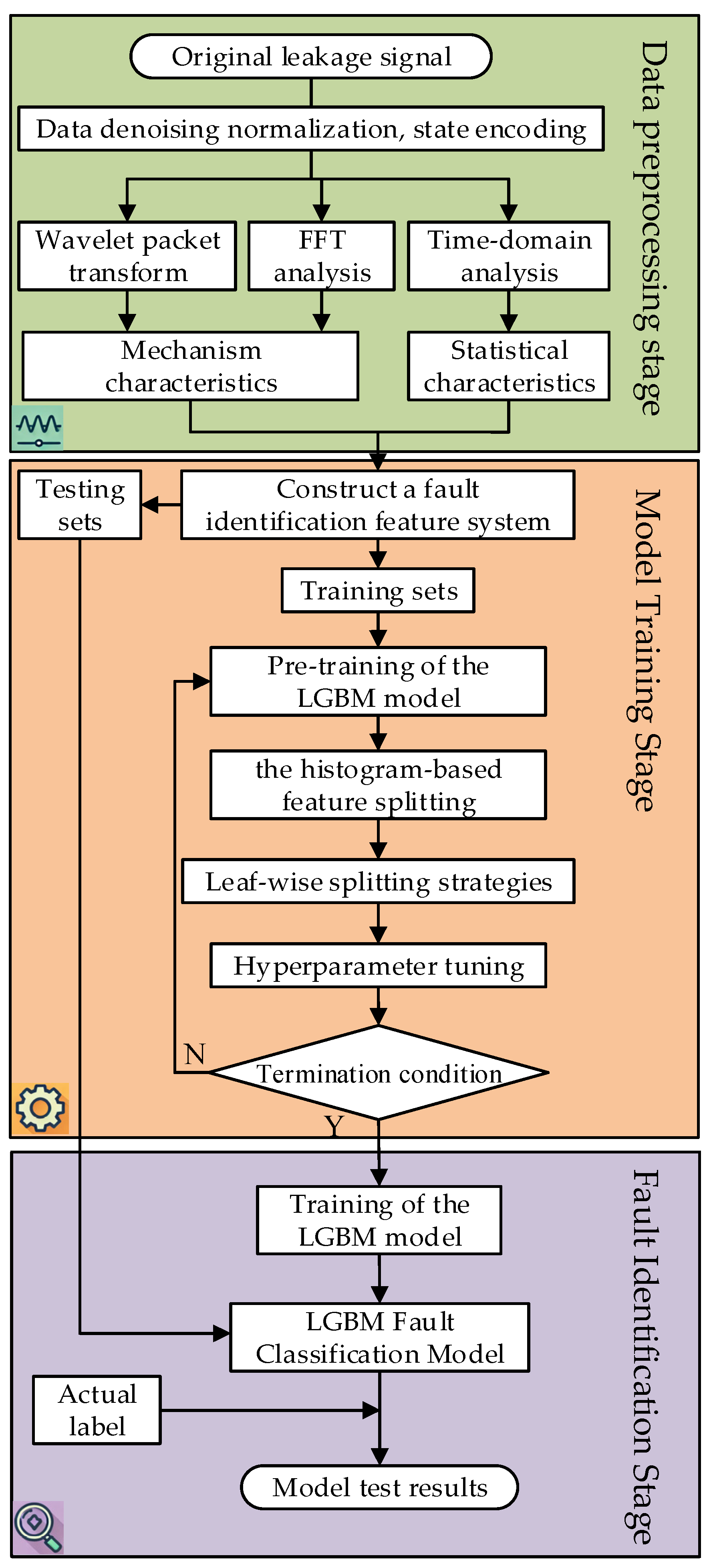
The fault type identification process for DC-side grounding faults in inverters based on LGBM is shown in Figure 12. The identification process mainly consists of the following three stages:
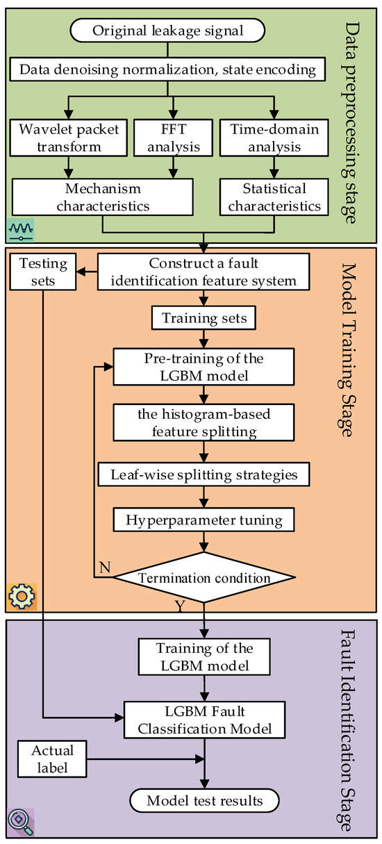
Figure 12.
Flowchart of DC-side grounding fault type identification in grid-connected inverters based on the LGBM model.
- Data Preprocessing Stage:
- ①
- Collect residual current data and preprocess it by denoising, normalization, and state encoding.
- ②
- Use wavelet packet transformation to reconstruct effective fault signals and extract residual current mechanism features through FFT analysis.
- ③
- Extract residual current statistical features through time-domain analysis.
- Model Training Stage:
- ④
- Construct a fault identification feature system, divide the dataset into training and testing sets by proportion, select a 12-dimensional feature vector as the model input, and use state encoding of different fault types as the model output.
- ⑤
- Perform initial hyperparameter configuration for pretraining based on model performance, utilizing the histogram-based feature splitting and leaf-wise splitting strategies to optimize the loss function through multiple iterations and constructing an efficient classification model.
- ⑥
- Use Bayesian optimization to simultaneously optimize multiple hyperparameters of the model, with the minimum training loss value as the termination condition, outputting the optimal hyperparameter values.
- Fault Identification Stage:
- ⑦
- Test the LGBM classification model using the test set and output the classification results.
- ⑧
- Combine the actual labels of the original dataset to obtain the final model testing results (classification accuracy).
6. Simulation Case Studies
6.1. Simulation Results
As shown in Table 6, two fault diagnosis models were designed in this study. LGBM1 is used to diagnose whether a leakage fault has occurred, while LGBM2 is used to identify the type of leakage fault in the inverter and determine the current fault type. Both LGBM1 and LGBM2 use eight mechanism features and four statistical features as input features.
Table 6.
Sample distribution and target output.
The output of LGBM1 is the diagnosis result, with target labels of 1 for “normal” and 0 for a “fault”. The output of LGBM2 corresponds to the four fault types, with target labels of 1, 2, 3, and 4, respectively.
An insufficient or excessive number of samples may lead to overfitting or impact the model’s performance, thereby reducing the accuracy of diagnosis and classification [31]. In this study, a total of 2500 samples were selected for the fault identification system’s training and testing. In order to improve the accuracy of the model, in this experiment, the five-fold cross-validation method was selected to process the training samples, avoiding the occurrence of overfitting during model training. The selected samples adequately represent the characteristics of all fault types. The samples were allocated using the following ratio: 80% for training and 20% for testing. Taking into account the complex working conditions under the irrational situation of the inverter grid-connected system, a small amount of fifth and seventh harmonic disturbances are added to the grid-connected power supply. Fault discrimination is carried out under such circumstances.
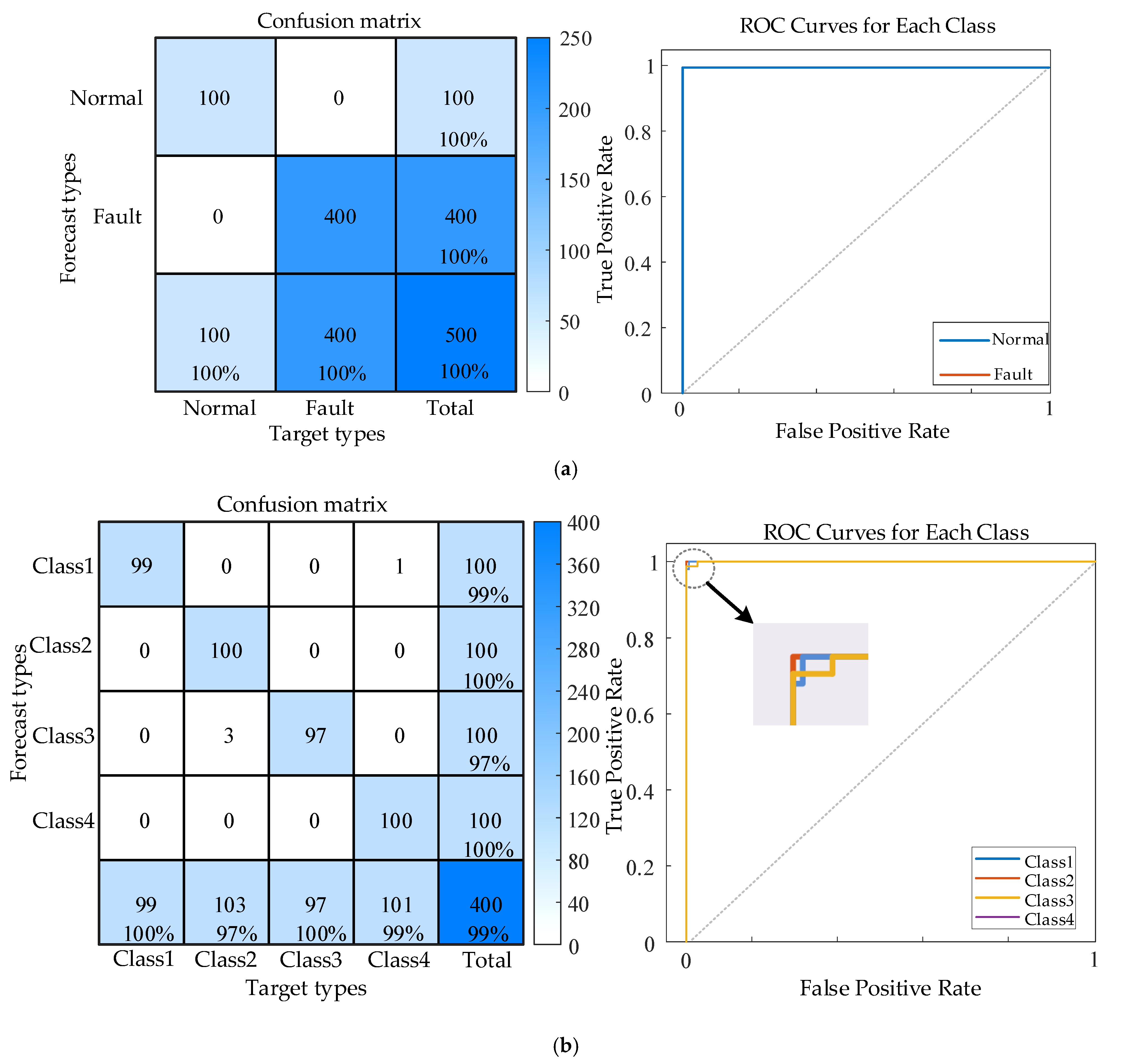
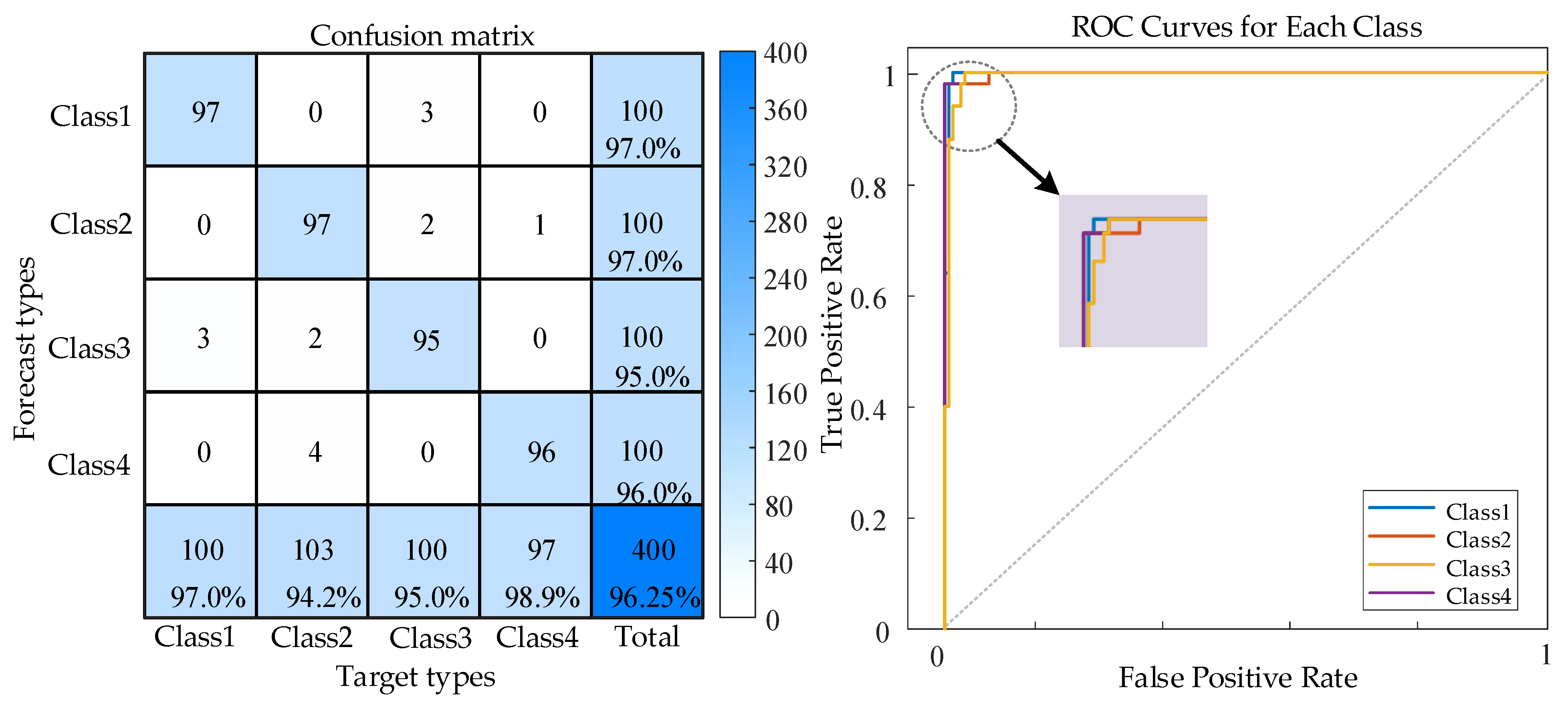
Since the test samples are entirely independent of the network training process, they can be used to verify whether the training results of the LGBM fault identification system meet expectations. By continuously optimizing the algorithm’s parameters, the best training performance was achieved, as shown in Figure 13. Figure 13 illustrates the model’s confusion matrix for testing and its receiver operating characteristic curve (ROC).
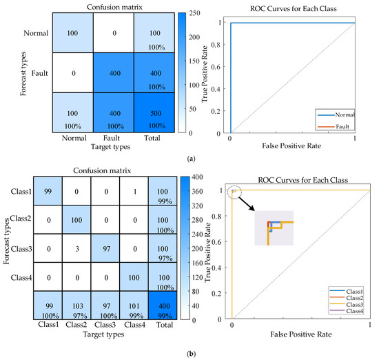
Figure 13.
Training results of the LGBM models. (a) Training results of LGBM1; (b) training results of LGBM2.
Figure 13a shows the results of leakage fault identification using statistical features and mechanism features as input parameters for the model. Among the 500 test samples, the fault identification accuracy reached 100%, and the ROC curve closely aligns with the top left corner, indicating extremely high accuracy in fault identification.
Figure 13b shows the classification results of leakage faults using statistical and mechanism features as input parameters for the model. In the 400 test sets, only four misclassifications occurred, and the fault classification accuracy rate reached 99.0%. This indicates that the combination of all features provides sufficient information to correctly distinguish each type of fault. The ROC curve is close to the upper left corner, suggesting that the classifier has extremely strong predictive ability for each category and that the error is very small. It shows that the combination of statistical features and mechanism features provides the richest information for fault identification and achieves the best classification effect.
To quantify the statistical uncertainty of the model’s predictions and verify the reliability of the results, this study introduces three quantitative indicators with a 95% confidence level: prediction interval coverage probability (PICP) to evaluate the confidence level of the diagnostic results, prediction interval normalized average width (PINAW) to characterize the prediction accuracy, and coverage width-based criterion (CWC) to comprehensively assess the quality of the intervals. The results are shown in Table 7.
Table 7.
Uncertainty quantification results of the fault identification model (at a 95% confidence level).
The results show that the PICP reaches 95.02%, fully meeting the requirements of a 95% confidence level, indicating that the model can reliably cover the actual fault characteristics. The PINAW is 0.097, suggesting that the prediction interval has high accuracy. The CWC value is 1.109851, close to the ideal value of 1, indicating that the model maintains a good interval width while ensuring coverage. These results collectively prove that our fault classification model not only can achieve accurate fault classification but also provides precise calibrated uncertainty estimation.
6.2. Comparison of Results for Different Feature Models
To validate the effectiveness and accuracy of the proposed method for identifying DC-side leakage faults in photovoltaic inverters based on mechanism features and statistical features, two different feature sets were used as input parameters for the model. These include the residual current mechanism features investigated in this study and the basic statistical features commonly used for fault type identification. The models were fitted using the same training dataset, and deep testing was conducted on the same test dataset. The testing results are shown in Figure 14 and Figure 15.

Figure 14.
Fault identification results using mechanism features with LGBM.
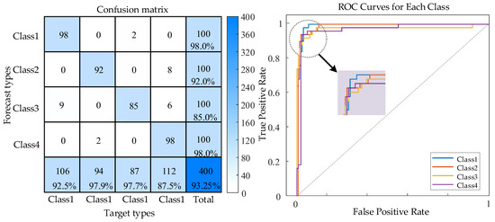
Figure 15.
Fault identification results using statistical features with LGBM.
Figure 14 shows the results of leakage fault classification when only mechanism features are used as input parameters for the model. The classification accuracy is 96.25%, with an increased misclassification rate for some categories, particularly between categories 3 and 4, where more confusion occurs. This results in a slight decline in accuracy compared to the proposed method. Although the overall trend of the ROC curve remains good, it exhibits slight fluctuations near the top left corner compared to Figure 12. The test results indicate that mechanism features can effectively represent fault types, but without the support of statistical features, the distinction between certain features is insufficient, leading to misclassification in some categories.
Figure 15 shows the results of leakage fault classification when only statistical features are used as input parameters for the model. The classification accuracy drops to 93.25%, significantly lower than the previous two cases, with more frequent misclassification, especially between categories 3 and 4, where the decline in recognition accuracy is more pronounced. The ROC curve performs noticeably worse than in the previous cases, with the curve being farther from the top left corner and exhibiting larger fluctuations, indicating weakened classification capability. When used alone, statistical features cannot sufficiently reflect the characteristics of different fault types. Therefore, relying solely on statistical features is insufficient to achieve high accuracy in leakage fault identification.
Table 8 presents a detailed comparison of the overall accuracy rate, AUC (area under the receiver operating characteristic curve), and training time of the algorithm under three different feature input scenarios. The results indicate that using both mechanism features and statistical features as model inputs yields the best leakage fault classification performance, with an accuracy of 99% and an AUC value of 0.988.
Table 8.
Comparison of indicators under different characteristics.
When only mechanism features are used, the leakage fault classification accuracy is 96.25%, and the AUC value is 0.981. However, there is more confusion in identifying fault types 3 and 4. When only statistical features are used, the leakage fault classification accuracy decreases significantly to 93.25%, with an AUC value of 0.958. This suggests that statistical features alone, without the support of mechanism features, struggle to effectively distinguish complex fault types. Meanwhile, in terms of the computational time of the algorithm, the differences among the three different feature selection methods are not significant. Therefore, choosing the fault classification method that combines mechanism features and statistical features will not affect the computational burden.
6.3. Model Feature Importance Visualization Analysis
The LGBM model, based on the gradient-boosting decision tree (GBDT) model, improves predictive performance by progressively optimizing decision trees. The LGBM model evaluates the importance of each feature by calculating its information gain, split frequency, and coverage in tree splits. The information gain reflects a feature’s contribution to optimizing the objective function, while the split frequency and coverage measure the frequency of a feature’s occurrence across all trees and its representativeness.
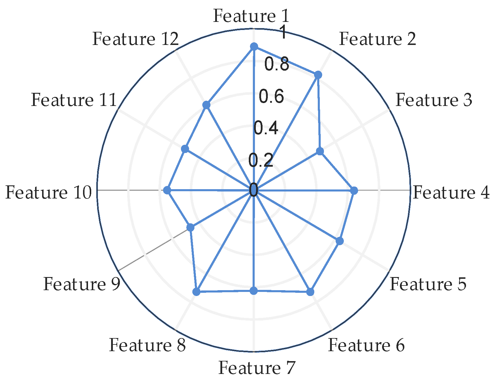
Using these metrics, the LGBM generates a feature importance distribution, enhancing the model’s interpretability. A radar chart can be used to quickly identify key features that critically impact the model and less important features, guiding feature selection and model optimization. Additionally, analyzing the significance of selected important features in the context of the leakage mechanism can validate the model’s predictions and enhance its interpretability, further supporting the reasoning behind the predictions. Figure 16 is a radar chart of the feature importance distribution.
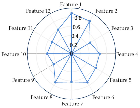
Figure 16.
Radar chart of the feature importance distribution.
Figure 17 presents the analysis results of the importance of each feature for the model output. The horizontal axis represents the normalized and averaged SHAP values, which are the comprehensive importance of the 12 features in contributing to the classification of the four fault types; the features are sorted from highest to lowest based on the average absolute SHAP value, with the features further up having a greater impact on the model’s prediction; in Figure 15, the color of each point represents the magnitude of the feature value (red for high values, blue for low values).
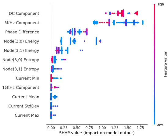
Figure 17.
SHAP summary plot for features.
As detailed in Table 4, the meanings of the 12 features are linked to their roles in leakage fault identification. Figure 16 and Figure 17 visually illustrate the distribution of feature importance within the model. Mechanism features (x1–x8) dominate the feature importance evaluation, highlighting their core role in the model’s classification and predictive capabilities. Among them, the DC component (x1) contributes the most and has an extremely strong ability to distinguish certain faults (such as capacitor series circuit faults); the high-frequency component (x2) reflects the high-frequency leakage current information caused by the switching effect and is of high importance. The wavelet information (x5–x8) and phase information (x4) capture local changes and the complex dynamics of the signal and are crucial for leakage fault identification.
The statistical features (x9–x12) rank lower and have a weak distinguishing effect. This might be due to the small distribution differences among different fault types, resulting in limited contributions to the classification task. These features reflect the overall statistical properties of the signal and are more suitable as supplementary features. Therefore, compared with statistical features, mechanism features have a higher importance, reflecting their physical significance and identification capabilities in power signal classification and better explaining the basis of model prediction.
6.4. Multi-Model Comparative Analysis
To demonstrate the effectiveness of the proposed model in identifying DC-side grounding faults in inverters, four mainstream classification and prediction models—BP, SVM, KNN, and XGBoost—were selected for comparison with the proposed model. These models were fitted using the same training dataset, and deep testing was conducted on the same test dataset. The feature selection for all models included the mechanism and statistical features listed in Table 4. The testing results are presented in Table 9.
Table 9.
Comparison of indicators under different algorithms.
Based on the test results in Table 9, the performance of different classification models in the task of DC-side grounding fault classification for inverters can be evaluated. The overall accuracy of the LGBM model is 99%, achieving perfect identification for all fault types and demonstrating outstanding performance. In comparison, other models such as BP (92.25%), SVM (81.5%), KNN (85.0%), and XGBoost (96.75%) show lower overall accuracies than LGBM, with SVM and KNN exhibiting particularly low classification accuracies for capacitive faults and resistive–capacitive series faults.
Beyond accuracy, the LGBM model also excels in efficiency, with a training time of just 1.161 s, which is faster than BP and comparable to XGBOOST, despite its higher complexity. This combination of high accuracy, balanced precision–recall, and computational efficiency makes LGBM the optimal choice for this fault classification task, outperforming traditional models (SVM and KNN) and even other boosting methods (XGBOOST).
Therefore, the superiority of LGBM lies in its ability to ensure 99% accuracy while maintaining relatively short training times, demonstrating high efficiency and stability. This makes it particularly suitable for inverter fault detection tasks that demand both high precision and efficiency.
7. Real-Time Simulation
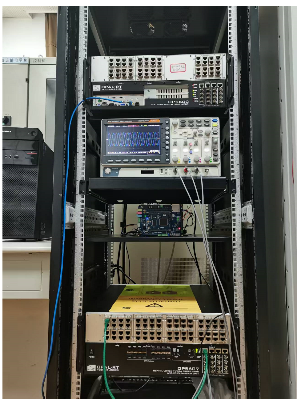
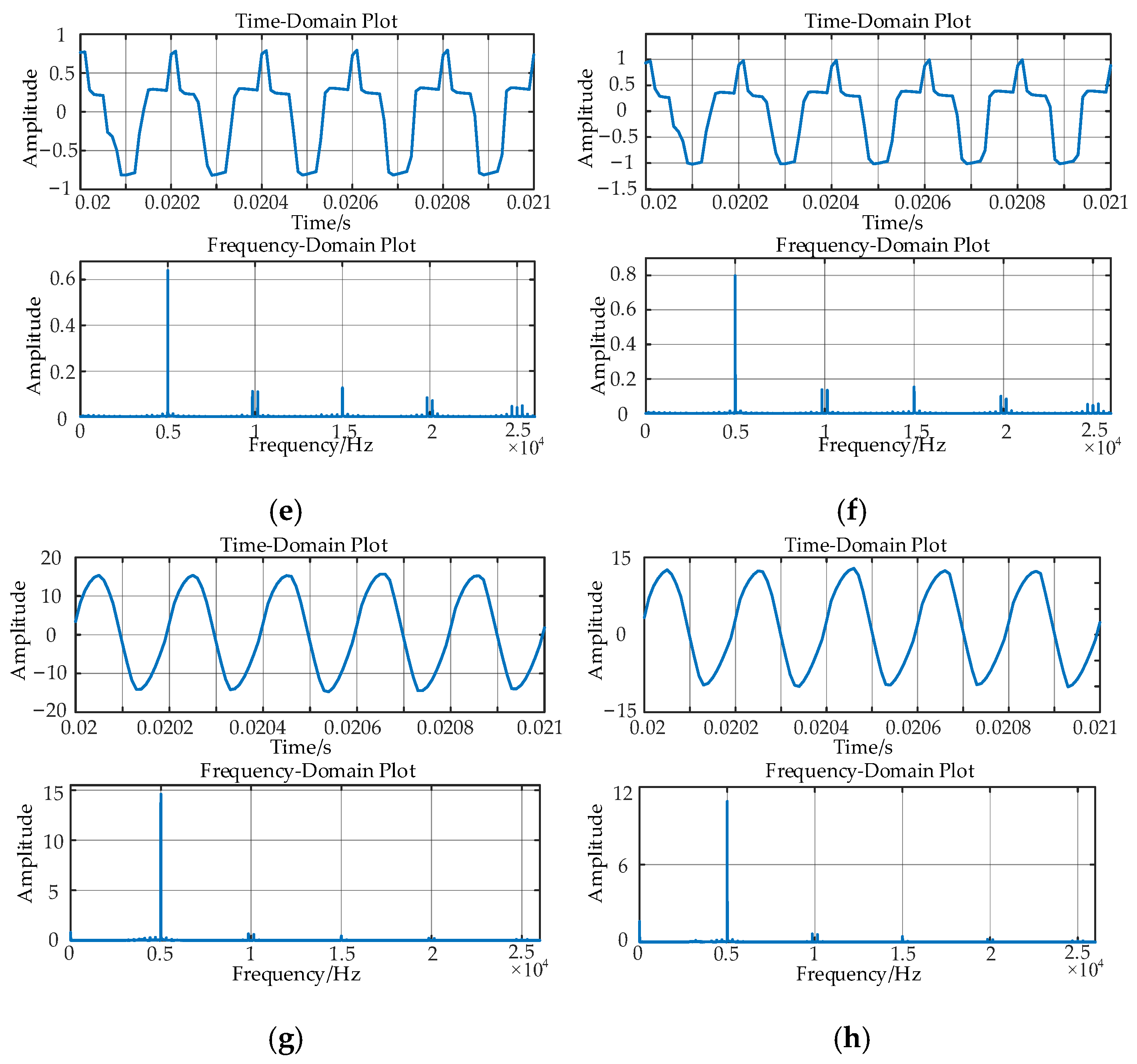
In order to further verify the validity and accuracy of the DC-side grounding fault discrimination method proposed in this paper, an RTLAB simulation experiment platform was constructed under the above-mentioned four different fault conditions. One case of each fault type was selected for fault discrimination experiments. The specific device is shown in Figure 18. The main circuit, including DC lines, capacitors, inductors, resistors, and power supplies, was constructed on the RTLAB platform. The specific parameters of the system are shown in Table 1. The parameters for pure resistance faults are as follows: (a) 500 Ω and (b) 300 Ω. For pure capacitance faults, the parameters are (c) 1 μF and (d) 1.5 μF. The parameters for series faults of resistance and capacitance are as follows: (e) 500 Ω, 1 μF; (f) 400 Ω, 1.2 μF. The parameters for parallel faults of resistance and capacitance are as follows: (e) 500 Ω, 1 μF; (f) 250 Ω, 1.3 μF.

Figure 18.
RTLAB experimental platform.
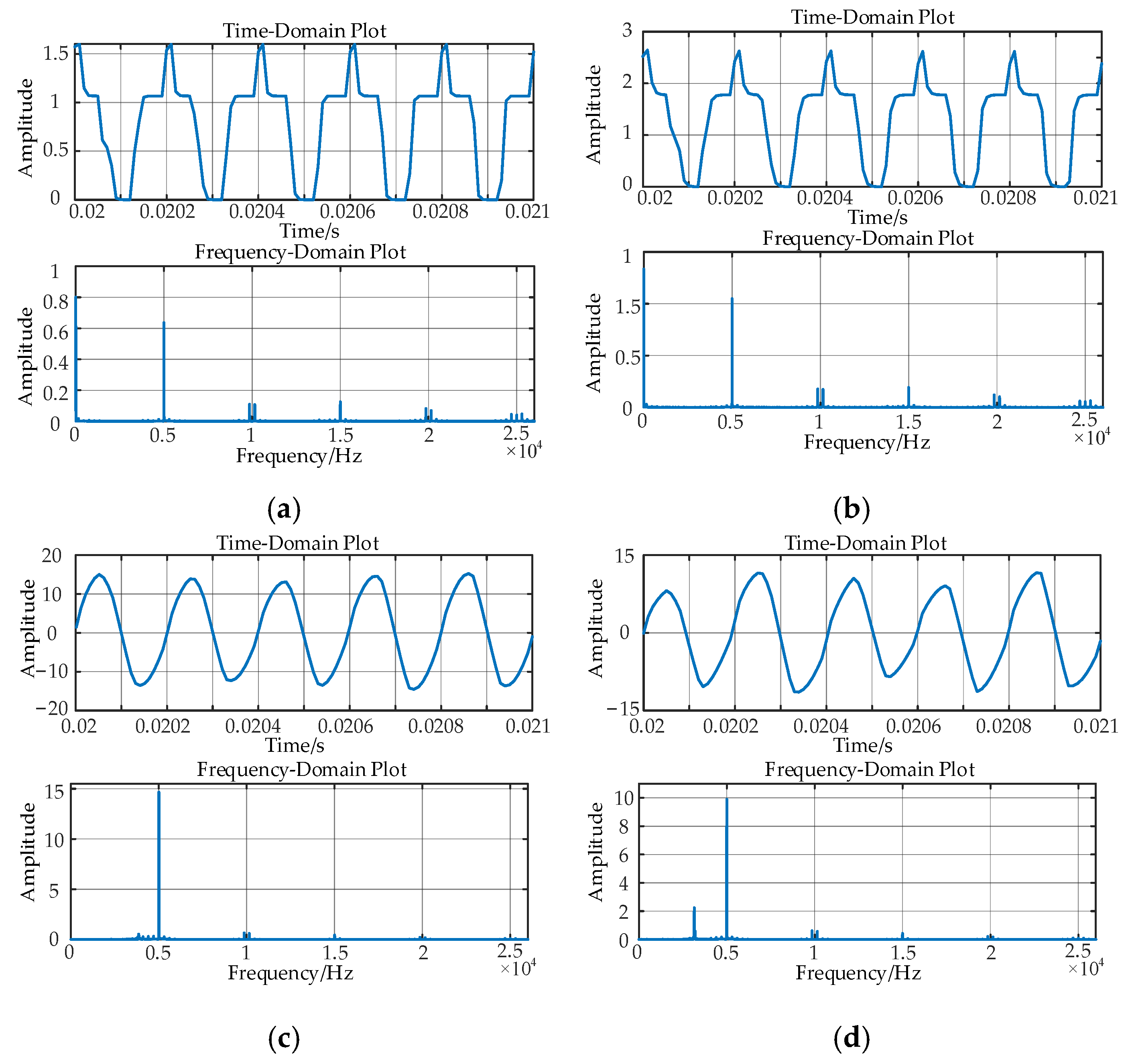
Figure 19 shows the time-domain and frequency-domain curves of the residual current under four fault types.
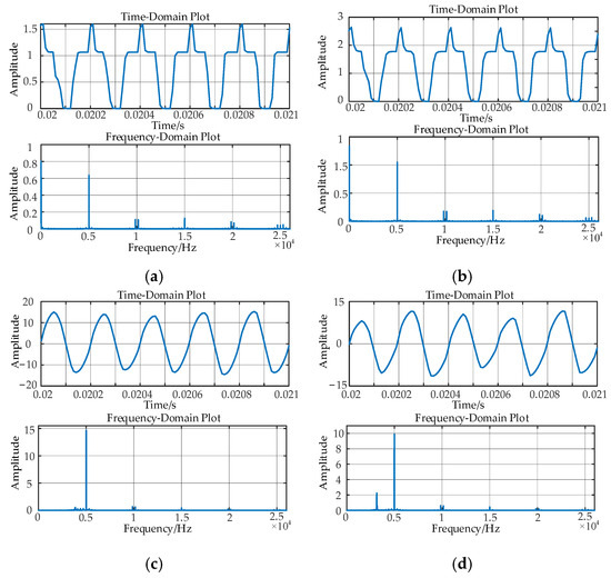
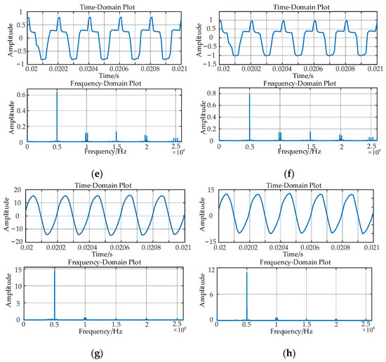
Figure 19.
Time-domain and frequency-domain curve diagrams of the residual current under four types of faults: (a,b) residual current waveform diagram under a resistance fault; (c,d) residual current waveform diagram under a capacitance fault; (e,f) residual current waveform diagram under a series connection of resistance and capacitance faults; and (g,h) residual current waveform diagram under a parallel connection of resistance and capacitance faults.
It can be clearly seen from Figure 19 that the frequency domain characteristics of the residual current for each fault type vary greatly. For example, in Figure 19a, where the fault is a resistance fault, the DC component and the 5KHz high-frequency component of the residual current are relatively large, while in Figure 19c, where the fault is a capacitance fault, the residual current has no DC component and the 5KHz high-frequency component has a very large value. Based on the verification of the experimental platform, it can be found that the four types of faults can be correctly identified. The specific results are shown in Table 10.
Table 10.
Fault type discrimination results.
8. Conclusions
This study focuses on a non-isolated three-phase grid-connected photovoltaic inverter, establishing an equivalent model for DC-side faults in the inverter system. The residual current generation mechanism and spectral characteristics were analyzed in depth, revealing the specific causes of different frequency components in the residual current. A fault identification method based on an LGBM was proposed by combining the mechanism features and statistical features of the residual current. This method provides theoretical and technical support for the rapid detection and identification of DC-side grounding faults in photovoltaic systems for practical engineering applications. The main conclusions are as follows:
- An equivalent leakage current model for the DC side of a non-isolated three-phase photovoltaic grid-connected inverter was constructed, revealing the characteristic that the leakage current is mainly formed by the combined action of two excitation sources (DC voltage and common-mode voltage).
- The residual current’s frequency domain, phase, and wavelet characteristics were analyzed under DC-side grounding faults in non-isolated three-phase photovoltaic inverters, uncovering the mechanism features of different leakage fault types. The results demonstrate significant differences in DC components, high-frequency components, phase characteristics, and wavelet information under various faults. These features effectively characterize the dynamic changes in residual current signals, offering reliable feature selection for fault type identification.
- A fault classification and identification method combining mechanism features and statistical features was proposed, along with a grounding fault identification process based on the LGBM algorithm. This method extracts mechanism features such as DC components, high-frequency harmonic components, phase information, and wavelet information, as well as commonly used statistical features, as model input variables. Bayesian optimization was employed to tune the LGBM model parameters. In simulation cases, the proposed method achieved a 99% accuracy rate for DC-side grounding fault identification and fault classification. Additionally, the feature importance visualization results indicate that mechanism features play a dominant role in model predictions, while statistical features enhance the model’s robustness as supplementary features. Compared with mainstream classification algorithms such as BP, SVM, KNN, and XGBoost, the proposed model demonstrates higher identification accuracy, stronger generalization ability, and shorter computation times. Experimental verification shows that introducing mechanism-based features into grid-connected photovoltaic inverters can significantly improve the accuracy of identifying grounding faults on the DC side.
- Future research directions can simulate more complex grid operation conditions to conduct fault discrimination on the DC side of inverters. For instance, factors such as sudden load changes, partial shading effects, three-phase imbalance, frequency deviation, and voltage fluctuation can be incorporated to enable the research in this paper to accurately identify faults on the DC side of inverters in more complex grid environments.
Author Contributions
Methodology, L.S.; Resources, C.K. and C.L.; Data curation, W.F.; Writing—review & editing, W.F. and C.L.; Visualization, M.W. All authors have read and agreed to the published version of the manuscript.
Funding
This research was supported by the National Grid Science and Technology Project, with the project number 521532240029.
Data Availability Statement
The original contributions presented in this study are included in the article. Further inquiries can be directed to the corresponding author.
Conflicts of Interest
The authors declare no conflict of interest.
References
- Khan, M.Y.A.; Liu, H.; Yang, Z.; Yuan, X. A Comprehensive Review on Grid-Connected Photovoltaic Inverters, Their Modulation Techniques, and Control Strategies. Energies 2020, 13, 4185. [Google Scholar] [CrossRef]
- Singh, T.S.D.; Shimray, B.A.; Meitei, S.N. Performance Analysis of a Rooftop Grid-Connected Photovoltaic System in North-Eastern India, Manipur. Energies 2025, 18, 1921. [Google Scholar] [CrossRef]
- Vodapally, S.N.; Ali, M.H. Overview of Intelligent Inverters and Associated Cybersecurity Issues for a Grid-Connected Solar Photovoltaic System. Energies 2023, 16, 5904. [Google Scholar] [CrossRef]
- Mumtaz, F.; Yahaya, N.Z.; Meraj, S.T.; Singh, B.; Kannan, R.; Ibrahim, O. Review on non-isolated DC-DC converters and their control techniques for renewable energy applications. Ain Shams Eng. J. 2021, 12, 3747–3763. [Google Scholar] [CrossRef]
- Yao, Z.; Zhang, Y.; Hu, X. Transformerless Grid-Connected PV Inverter Without Common Mode Leakage Current and Shoot-Through Problems. IEEE Trans. Circuits Syst. II Express Briefs 2020, 67, 3562–3566. [Google Scholar] [CrossRef]
- DIN VDE 0126-1-1-2006; Automatic Disconnection Device Between a Generator and the Public Low-Voltage Grid. DKE: Frankfurt, Germany, 2008.
- NB/T 32004-2013; Technical Specification of Grid-Connected PV Inverter. China Electric Power Press: Beijing, China, 2013.
- Ling, F.; Ma, M.; Sun, Y.; Long, H.; Li, F. Design of general framework for multi-fault diagnosis based on photovoltaic grid-connected inverter system. In Proceedings of the 8th Renewable Power Generation Conference (RPG 2019), Shanghai, China, 24–25 October 2019. [Google Scholar] [CrossRef]
- Zhao, D.; He, S.; Huang, H.; Han, Z.; Cui, L.; Li, Y. Strategy for Suppressing Commutation Failures in High-Voltage Direct Current Inverter Station Based on Transient Overvoltage. Energies 2024, 17, 1094. [Google Scholar] [CrossRef]
- Khodja, M.E.A.; Aimer, A.F.; Boudinar, A.H.; Benouzza, N.; Bendiabdellah, A. Bearing fault diagnosis of a PWM inverter fed-induction motor using an improved short time Fourier transform. J. Electr. Eng. Technol. 2019, 14, 1201–1210. [Google Scholar] [CrossRef]
- Mishra, M.; Rout, P.K. Detection and classification of micro-grid faults based on HHT and machine learning techniques. IET Gener. Transm. Distrib. 2018, 12, 388–397. [Google Scholar] [CrossRef]
- Iglesias-Rojas, J.C.; Velázquez-Lozada, E.; Baca-Arroyo, R. Online Failure Diagnostic in Full-Bridge Module for Optimum Setup of an IGBT-Based Multilevel Inverter. Energies 2022, 15, 5203. [Google Scholar] [CrossRef]
- Wang, B.; Feng, X.; Wang, R. Open-Circuit Fault Diagnosis for Permanent Magnet Synchronous Motor Drives Based on Voltage Residual Analysis. Energies 2023, 16, 5722. [Google Scholar] [CrossRef]
- Liu, C.; Zhuo, F.; Wang, F. Fault Diagnosis of Commutation Failure Using Wavelet Transform and Wavelet Neural Network in HVDC Transmission System. IEEE Trans. Instrum. Meas. 2021, 70, 1–8. [Google Scholar] [CrossRef]
- Kumar, G.K.; Parimalasundar, E.; Elangovan, D.; Sanjeevikumar, P.; Lannuzzo, F.; Holm-Nielsen, J.B. Fault Investigation in Cascaded H-Bridge Multilevel Inverter through Fast Fourier Transform and Artificial Neural Network Approach. Energies 2020, 13, 1299. [Google Scholar] [CrossRef]
- Wang, L.; Wu, Z.; Zhou, L.; Kang, J. Analysis of DC bus overvoltage in parallel photovoltaic systems. In Proceedings of the 18th International Conference on Electrical Machines and Systems (ICEMS), Pattaya, Thailand, 25–28 October 2015; pp. 1074–1079. [Google Scholar] [CrossRef]
- Lee, J.; Lee, K. Open-Switch Fault Detection Method of a Back-to-Back Converter Using 72 NPC Topology for Wind Turbine Systems. IEEE Trans. Ind. Appl. 2015, 51, 325–335. [Google Scholar] [CrossRef]
- Jia, K.; Christopher, E.; Thomas, D. Advanced DC zonal marine power system protection. IET Gener. Transm. Distrib. 2014, 8, 301–309. [Google Scholar] [CrossRef]
- Farnesi, S.; Fazio, P.; Marchesoni, M. A new fault tolerant NPC converter system for high power induction motor drives. In Proceedings of the 8th IEEE Symposium on Diagnostics for Electrical Machines, Power Electronics & Drives (SDEMPED), Bologna, Italy, 5–8 September 2011; pp. 337–343. [Google Scholar] [CrossRef]
- Hu, C.; Jiang, Y.; Ling, Z. Research on Fault Diagnosis of Three-Level Photovoltaic Inverter. Sci. Technol. Vis. 2014, 82. [Google Scholar] [CrossRef]
- Abari, I.; Hamouda, M.; Slama, J.B.H. Open-switch fault detection in three-phase symmetrical cascaded multilevel inverter using conducted disturbances. In Proceedings of the 15th International Multi-Conference on Systems, Signals & Devices (SSD), Hammamet, Tunisia, 19–22 March 2018; pp. 77–82. [Google Scholar] [CrossRef]
- Abari, I.; Lahouar, A.; Hamouda, M. Fault detection methods for three-level NPC inverter based on DC-bus electromagnetic signatures. IEEE Trans. Ind. Electron. 2018, 65, 5224–5236. [Google Scholar] [CrossRef]
- Amaral, T.G.; Pires, V.F.; Cordeiro, A.; Foito, D.; Martins, J.F.; Yamnenko, J.; Tereschenko, T.; Laikova, L.; Fedin, I. Incipient Fault Diagnosis of a Grid-Connected T-Type Multilevel Inverter Using Multilayer Perceptron and Walsh Transform. Energies 2023, 16, 2668. [Google Scholar] [CrossRef]
- Khomfoi, S.; Tolbert, L.M. Fault diagnosis and reconfiguration for multilevel inverter drive using AI-based techniques. IEEE Trans. Ind. Electron. 2007, 54, 2954–2968. [Google Scholar] [CrossRef]
- Cui, J.; Shi, G.; Gong, C. A fast classification method of faults in power electronic circuits based on support vector machines. Metrol. Meas. Syst. 2017, 24, 701–720. [Google Scholar] [CrossRef]
- Guo, Y.; Wu, W.; Lin, Q.; Cai, F.; Chai, Q. Fault diagnosis for power converters based on optimized temporal convolutional network. IEEE Trans. Instrum. Meas. 2020, 70, 1–10. [Google Scholar] [CrossRef]
- Wang, M.; Shen, K.; Tai, C.; Zhang, Q.; Yang, Z.; Guo, C.; Gupta, B.B. Research on fault diagnosis system for belt conveyor based on internet of things and the LightGBM model. PLoS ONE 2023, 18, e0277352. [Google Scholar] [CrossRef] [PubMed]
- Li, G.; Li, W.; Wen, T.; Sun, W.; Tang, X. High-Dimensional Feature Fault Diagnosis Method Based on HEFS-LGBM. J. Electron. Test. 2024, 40, 557–572. [Google Scholar] [CrossRef]
- Jahan, S.; Kibria, M.F.; Biswas, S.P.; Islam, M.R.; Rahman, M.A.; Muttaqi, K.M. H9 and H10 Transformer-Less Solar Photovoltaic Inverters for Leakage Current Suppression and Harmonic Current Reduction. IEEE Trans. Ind. Appl. 2023, 59, 2446–2457. [Google Scholar] [CrossRef]
- Morales-Caporal, R.; Pérez-Cuapio, J.F.; Martínez-Hernández, H.P. Design and hardware implementation of a H-bridge sub-module for single-phase 5-level cascaded voltage source inverters. In Proceedings of the IECON 2021—47th Annual Conference of the IEEE Industrial Electronics Society, Toronto, ON, Canada, 13–16 October 2021; pp. 1–6. [Google Scholar] [CrossRef]
- He, C.M.; Li, X.G.; Xia, Y.; Tang, J.; Yang, J.; Ye, Z. Addressing the Overfitting in Partial Domain Adaptation With Self-Training and Contrastive Learning. IEEE Trans. Circuits Syst. Video Technol. 2024, 34, 1532–1545. [Google Scholar] [CrossRef]


Disclaimer/Publisher’s Note: The statements, opinions and data contained in all publications are solely those of the individual author(s) and contributor(s) and not of MDPI and/or the editor(s). MDPI and/or the editor(s) disclaim responsibility for any injury to people or property resulting from any ideas, methods, instructions or products referred to in the content. |
© 2025 by the authors. Licensee MDPI, Basel, Switzerland. This article is an open access article distributed under the terms and conditions of the Creative Commons Attribution (CC BY) license (https://creativecommons.org/licenses/by/4.0/).