Impact of Daylight Saving Time on Energy Consumption in Higher Education Institutions: A Case Study of Portugal and Spain

Abstract

Daylight Saving Time (DST), involving clock shifts forward in spring and backward in autumn, was introduced to promote energy savings. However, its effectiveness remains controversial, especially in buildings with temporary occupancy like academic institutions, which have high daytime use but low summer occupancy. This study investigates the impact of DST transitions on energy consumption across seven campuses of two higher education institutions (HEIs) in northern Portugal and Spain, located in different time zones, using measured data from 2023. The analysis accounted for the structural and operational characteristics of each campus to contextualize consumption patterns. Weekly electricity consumption before and after DST changes were compared using independent samples t-tests to assess statistical significance. Results show that the spring transition to DST led to an average energy saving of 1.7%, while the autumn return to standard time caused an average increase of 1.2%. Significant differences (p < 0.05) were found in five of the seven campuses. Descriptive statistics and confidence intervals indicated that only sites with intervals excluding zero exhibited consistent changes. Seasonal energy demand appeared more influenced by academic schedules and thermal comfort needs—particularly heating—than by DST alone. Higher consumption coincided with periods of intense academic activity and extreme temperatures, while lower demand aligned with holidays and longer daylight months. Although DST yielded modest energy savings, its overall impact on academic campus energy use is limited and highly dependent on local conditions. The findings highlight the need to consider regional climate, institutional policies, user behavior, and smart technology integration in future energy efficiency analyses in academic settings.

1. Introduction

Daylight Saving Time (DST) has been implemented in many countries as a strategy to reduce energy consumption during summer months by shifting daylight to later hours of the day. The rationale is that increased evening daylight decreases the need for artificial lighting. However, the actual effectiveness of DST remains debated, with mixed evidence from the literature and ongoing policy discussions—such as the 2018 proposal by the European Union to abolish seasonal time changes [1,2]. The impact of DST on energy use is influenced by various contextual factors, including regional climate, building characteristics, social routines, and sector-specific activity profiles. Higher Education Institutions (HEIs) are particularly relevant for investigation due to their complex infrastructures and substantial energy demands driven by strict requirements for indoor air quality, thermal comfort, and energy certification standards [3]. Despite their significance, research focusing specifically on DST’s effect within HEIs is limited and inconclusive. Some studies report modest energy savings, while others observe increased consumption resulting from compensatory heating or cooling needs, especially in regions with pronounced seasonal climate variation. Factors such as latitude, occupancy schedules, and building thermal inertia contribute to these divergent results. Moreover, most existing research tends to focus on residential or commercial buildings, with few studies examining educational campuses, and even fewer comparing adjacent regions with differing time zone policies but similar climatic conditions. This gap leaves unclear how DST affects energy consumption in HEIs operating under different time regimes but comparable environmental settings.

This study addresses the identified research gap—the limited and inconclusive analysis of Daylight Saving Time (DST) effects within Higher Education Institutions (HEIs)—by analyzing electricity consumption data from university buildings across two geographically close HEIs in Northern Portugal and Spain. These institutions share similar climatic conditions but operate under different time zone policies, offering a unique opportunity to assess the real-world impact of DST transitions on energy consumption in academic settings.

2. Literature Review

The literature review supporting this work was based on publications indexed in the SCOPUS database, which was selected due to its extensive coverage in the areas of energy, environmental sciences, and engineering, as well as for institutional access and consistency with prior research methodologies. Although other databases such as Web of Science (WOS) were not included in the search, existing comparative studies have shown a high degree of overlap between SCOPUS and WOS in these disciplines. As such, we believe the coverage achieved is sufficiently representative for this study. The relationship between Daylight Saving Time (DST) and energy consumption has been extensively studied, yet results remain inconclusive and highly dependent on contextual variables. Originally proposed as a policy measure to better align human activity with daylight hours and reduce the need for artificial lighting, DST was expected to offer substantial benefits in terms of energy efficiency. However, empirical findings show that actual energy savings are often modest, inconsistent, or even negative, with some regions experiencing an increase in overall consumption. This paradox arises due to various interacting factors, such as geographic latitude, climate conditions, daylight availability, social behavior, energy pricing, and infrastructure characteristics. For instance, while the extension of daylight hours in the evening may reduce the need for lighting, it can simultaneously increase demand for air conditioning during hotter periods or for heating during colder mornings. Moreover, changes in peak demand profiles may have complex implications for grid stability and energy costs. Despite the policy relevance of DST, especially in light of global energy sustainability goals, there remains a limited body of research focused specifically on its effects within the context of Higher Education Institutions (HEIs), which often exhibit distinctive energy consumption patterns due to their diverse spaces (e.g., laboratories, lecture halls, dormitories), high occupancy variability, and seasonally driven academic calendars.

To address this gap and assess the scientific discourse on DST and energy consumption, a bibliometric review was conducted using data extracted from the Scopus database. The analysis was carried out with the Bibliometrix package in RStudio, version 2024.04.2+764, a robust tool designed for quantitative exploration of academic literature. A total of 48 documents were retrieved using the keywords “daylight saving time” and “energy”, covering a span from 1977 to 2024. After filtering for peer-reviewed articles, 36 studies were selected for deeper analysis. The data were exported in BIB format and processed to extract metadata, citation patterns, and thematic structures.

The temporal distribution of scientific output on daylight saving time (DST) and its impact on energy consumption reveals a sporadic pattern in the early decades, with isolated publications in the 1970s and 1990s. A noticeable increase in research activity began in the mid-2000s, coinciding with growing global interest in energy efficiency and climate policy. A significant peak occurred in 2020, potentially reflecting heightened public debate and policy review processes related to DST.

Figure 1 presents the annual scientific production on this topic from 1976 to 2024.

Other years with notable outputs include 2008, 2011, 2018, 2021, and 2024, indicating consistent interest over time. Citation analysis revealed that the most influential article was by ARIES MBC (2008), published in Energy Policy, followed by other significant contributions appearing in journals from fields as diverse as neuroscience, public safety, and environmental science—demonstrating the interdisciplinary nature of DST research.

Thematic mapping enabled a clearer understanding of how the field is structured conceptually. Using measures of centrality (relevance within the field) and density (development of the topic), themes were categorized into four quadrants. “Motor themes”, such as energy efficiency, electricity consumption, and energy conservation, emerged as central and well-developed, indicating their foundational importance to the field. “Niche themes”, including physiological effects and traffic-related outcomes, were specialized but less connected to broader debates. “Basic themes”, like demographic categorizations and regional analyses, were central yet underdeveloped, suggesting room for deeper theoretical grounding. Meanwhile, “emerging or declining themes”, such as simulation models and computational methods, reflected newer directions in the literature that may gain prominence as analytical tools evolve and as policy interest in energy modeling increases. Keyword co-occurrence analysis further revealed the conceptual interlinkages in the literature, identifying clusters of terms that frequently appear together, thus illustrating the major research threads and suggesting potential integration points between currently disconnected subfields.

Numerous empirical studies were reviewed to evaluate the real-world impact of DST on energy consumption across different geographical and economic contexts. For instance, Kudela et al. (2020) reported a modest 0.5% annual electricity saving in Slovakia [3]. Flores et al. (2019) used a difference-in-differences econometric approach to analyze Mexican residential consumption, revealing a 0.6% reduction, though the effect was uneven over time [4]. In Brazil, Petterini et al. (2018) found that DST yielded notable savings in Bahia but minimal changes in Tocantins, illustrating the role of regional characteristics in mediating DST’s effects [5]. In Western Australia, Choi et al. (2017) observed no significant reduction in overall electricity use, despite reductions during peak demand periods [6]. Ahuja and SenGupta (2012) proposed a year-round DST model for India, hypothesizing energy gains by shifting the national time zone to UTC+6:00, while Guven et al. (2021) highlighted the crucial role of local temperature and climate in determining the outcome of DST policies [7,8]. In colder regions such as Norway and Sweden, Mirza and Bergland (2011) reported consistent, albeit small, energy reductions concentrated during evening hours, echoing findings from Havranek et al. (2018), whose meta-analysis estimated global average savings at just 0.34%, with stronger effects in higher latitudes [9,10].

Simulation-based analyses also present contrasting perspectives. Rock (1997), through residential building models in the U.S., found that DST slightly increased energy usage due to HVAC demand [11]. Similarly, studies by López (2020) in Spain and Chen et al. (2024) in China demonstrated that while DST can influence daily load profiles, the net effect depends heavily on the policy scenario and regional climatic conditions [12,13]. Krarti and Hajiah (2011) analyzed buildings in Kuwait and found mixed outcomes: minor savings in commercial sectors but increased residential consumption [14]. Meanwhile, Eggimann et al. (2023) reported that office buildings in the U.S. benefitted from decreased cooling loads during DST, which outweighed the slight increase in heating requirements [15].

In conclusion, although DST can provide energy savings under specific conditions, its overall effectiveness remains variable and highly context-specific. While countries at higher latitudes and with particular usage profiles might benefit modestly, the impacts in equatorial or warmer climates can be negligible or counterproductive. The literature also indicates that the nature of energy savings has shifted over time: whereas earlier policies primarily aimed to reduce lighting loads, modern energy demands are increasingly driven by heating, cooling, and electronics, which complicates the efficacy of simple clock shifts. The role of social habits, building technologies, and policy enforcement further adds to the complexity. Within this landscape, HEIs represent a particularly underexplored yet promising context for analysis, given their structural complexity, long daily operating hours, and diverse energy uses. Expanding research in this area is essential for understanding the nuanced effects of DST and for informing more precise, data-driven energy policies tailored to institutional settings.

Summary of Bibliographic Review on DST Effect on Energy Consumption

Numerous studies have explored the impact of Daylight Saving Time (DST) on electricity consumption, employing diverse methodologies and focusing on various geographic and climatic contexts. Kudela et al. (2020) examined DST’s effect in Slovakia and concluded that DST results in modest electricity savings of around 0.5% of annual consumption [3]. Similarly, Flores et al. (2019) utilized a difference-in-differences econometric approach to evaluate residential electricity consumption in Mexico and found a reduction of 0.6%, although the effect was not consistent throughout the analyzed period [4]. Petterini et al. (2018) analyzed state-level energy consumption in Brazil and found that DST led to significant energy savings in Bahia but minimal effects in Tocantins [5]. In contrast, Choi et al. (2017) studied data from Western Australia and concluded that DST did not significantly reduce overall electricity consumption, despite reducing demand during peak hours [6]. Ahuja and SenGupta (2012) proposed a year-round DST policy for India, arguing that aligning the clock with UTC+6:00 would yield substantial energy savings [7]. Similarly, Rock (1997) utilized simulation models for U.S. residential buildings and found that DST slightly increased energy consumption due to heightened HVAC use [11]. López (2020) focused on Spain, showing that DST impacts daily load profiles, and savings vary based on policy scenarios [12]. In the Middle East, Krarti and Hajiah (2011) assessed the building sector in Kuwait and found mixed effects, with slight energy savings in commercial sectors but increased consumption in private residences [14]. Momami et al. (2009) observed marginal reductions in electricity consumption in Jordan, primarily in lighting loads [16]. Studies in higher latitudes, such as those by Mirza and Bergland (2011) in Norway and Sweden, reported annual reductions of up to 1% in electricity use, with savings concentrated during evening hours [9]. Similarly, Havranek et al. (2018) conducted a meta-analysis and highlighted that savings were greater in regions farther from the equator, though overall reductions were modest at 0.34% [10]. In Australia, Kellogg and Wolff (2008) and Guven et al. (2021) both highlighted the nuanced effects of DST [8,17]. While the former noted limited overall reductions, the latter emphasized the importance of weather conditions and cooling usage in determining DST’s energy-saving potential [8,17]. In Turkey, Karasu (2010) and Bircan and Wirsching (2023) demonstrated that adopting DST or similar policies could yield small but measurable reductions in electricity demand, especially in lighting [18,19]. Similarly, Eggimann et al. (2023) studied office buildings across the United States and found that DST reduces cooling energy demand more than it increases heating [15]. Finally, studies in Europe, such as Bellia et al. (2020), emphasized that DST’s effectiveness depends on latitude and luminous climate [20], while Chen et al. (2024) demonstrated modest reductions in household lighting energy in China, particularly in northern cities [13]. Other studies have examined the complex relationship between daylight saving time (DST), building energy use, and contextual factors such as climate, building typology, and occupant behavior. While the results remain inconclusive, there is growing recognition that behavioral patterns and passive design features play a crucial role in energy dynamics, especially in educational settings. For instance, Niima Essakali et al. (2025) investigated energy use in rural schools through multi-objective passive design optimization strategies, including bio-based insulation, shading, and vegetative roofing, to improve thermal performance under climatic constraints [21]. Although their work focused on rural schools rather than higher education buildings, it highlights the importance of integrating climate-responsive strategies and occupant-driven usage patterns—elements also relevant to understanding DST-related impacts in institutional buildings.

In summary, while DST generally results in small energy savings, its effectiveness depends on geographic, climatic, and policy factors [13]. Savings are typically higher in regions farther from the equator and during specific periods, though they may be offset by increased demand for heating or cooling. These articles and results are summarized in

Table 1. Summary of DST bibliographic review.

Reference	Title	Country	Key Findings
Kudela et al. (2020) [3]	Does daylight saving time save electricity? Evidence from Slovakia	Slovakia	DST led to a modest reduction in electricity consumption, estimated at about 0.8% of annual electricity use.
Daniel Flores et al. (2019) [4]	An Econometric Evaluation of Daylight Saving Time in Mexico	México	DST leads to modest electricity savings, amounting to around 0.6% of total national electricity consumption.
Francis Petterini et al. (2018) [5]	The Limitation of Daylight Saving Time: Quasi-Experimental Analyses of Electricity Consumption in Bahia and Tocantins	Brazil	DST may have minimal impact on reducing electricity consumption in these states.
Choi et al. (2017) [6]	How does daylight saving time affect electricity demand? An answer using aggregate data from a natural experiment in Western Australia	Australia	DST did not significantly reduce overall electricity consumption.
Ahuja and SenGupta (2012) [7]	Year-round Daylight Saving Time Will Save More Energy In India Than Corresponding DST Or Time Zones	India	DST could result in greater energy savings compared to seasonal DST or altering the country’s time zones for India.
Brian Rock (1997) [11]	Impact of daylight saving time on residential energy consumption and cost	U.S.	DST results in a slight increase, rather than a decrease, in total residential energy consumption.
Miguel López (2020) [12]	Daylight Effect on the electricity Demand In Spain And Assessment of Daylight Saving Time Policies	Spain	Changes in sunrise and sunset times affect daily load profiles.
Krarti and Hajiah (2011) [14]	Analyses Of The Impact Of Daylight Time Savings On Energy Use Of Buildings In Kuwait	Kuwait	DST reduces the demand for lighting and air conditioning during the longer daylight hours.
Tomas Havranek yet al. (2018) [10]	Does Daylight Saving Save Electricity? A Meta-Analysis	Various	DST does result in small reductions in electricity consumption and might be offset by increased energy use elsewhere (e.g., heating or air conditioning).
Mirza and Bergland (2011) [9]	The Impact Of Daylight Saving Time On Electricity Consumption: Evidence From Southern Norway And Sweden	Norway and Sweden	Limited or modest reductions in electricity consumption due to DST, primarily in the evening hours.
Momami et al. (2009) [16]	The impact of the Daylight Saving Time On Electricity Consumption - A Case Study From Jordan	Jordan	Marginal reductions in electricity consumption, especially in terms of lighting demand during the longer daylight hours in the evening.
Kellogg and Wolff (2008) [17]	Daylight Time and Energy: Evidence from an Australian Experiment	Australia	Small reduction in electricity consumption, mainly due to decreased lighting needs during the extended daylight hours in the evening.
Servet Karasu (2010) [18]	The Effect of Daylight Saving Time Options On The Electricity Consumption Of Turkey	Turkey	DST reduces the demand for electricity, especially for lighting, during the extended daylight hours in the evening.
Guven et al. (2021) [8]	When Does Daylight Saving Time Save Electricity? Weather and Air-Conditioning	Australia	DST impact on electricity savings is highly dependent on weather conditions.
Bircan and Wirsching (2023) [19]	Daylight saving all year round? Evidence from a national experiment	Turkey	Adopting DST year-round could lead to small but sustained energy savings.
Eggimann et al. (2023) [15]	Climate change shifts the trade-off between lower cooling and higher heating demand from daylight saving time in office buildings	U.S.	Maximum savings of up to 5.9% for cooling and a 4.4% increase in heating.
Bellia et al. (2020) [20]	Impact of daylight saving time on lighting energy consumption and on the biological clock for occupants in office buildings	Europe	DST leads to a decrease in lighting energy consumption in office buildings by extending daylight into the evening, reducing the need for artificial lighting.
Chen et al. (2024) [13]	Evaluation of the effect of daylight saving time on household	China	DST leads to modest energy savings for households, primarily due to a reduction in lighting usage during extended evening daylight hours.

.

3. Materials and Methods

3.1. Analyzed Consumption Data

This study employs a quantitative approach to analyze energy consumption data from multiple school buildings in the North of Portugal and Spain, during periods with and without daylight saving time enforcement, allowing for the systematic measurement, comparison, and evaluation of consumption patterns across different buildings and time periods. The data are obtained directly from the load diagrams of each delivery point and correspond to the year 2023. Typically produced by energy suppliers, these load diagrams record electricity consumption at regular one-hour intervals throughout the year, providing high-resolution insight into the temporal patterns of energy demand.

3.2. Case Study

This case study aims to analyze the annual consumption of seven buildings belonging to two higher education institutions: Polytechnic University of Viana do Castelo, in Portugal, and University of Vigo, in Spain. Six of the buildings studied are located in the district of Viana do Castelo, Portugal, and one in Vigo, in the province of Pontevedra, Galicia, Spain, as shown in Figure 2. Although they have a similar geography and are separated by a very short distance, the time difference between the two countries is one hour, as continental Spain has Central European Time (CET) and continental Portugal has one hour less, both in summer and in winter.

Table 2. Summary of main characteristics of the buildings under analysis.

Building	Year of Construction	Total Floor Area (m2)	Users	Energy Certificate	PV System	Consumption (PV + GRID) kWh
ESCEV	2016	5990	751	B-	na	170,377
ESDLM	2013	5430	526	na	na	108,548
ESAPL	1989; 1992	9458	764	A	54.7 kWp	358,113
ESEVC	1986; 1999; 2003	9510	1002	C	na	210,612
ESSVC	1995; 2011	6915	554	A	57.8 kWp	198,963
ESTGVC	1992	12,610	3178	A	102.8 kWp	429,549
UVEM	2005	9000	600	na	102 kWp	322,402

provides a comparative overview of the seven buildings analyzed, highlighting differences in building size, campus population, building energy certification level, installed photovoltaic (PV) system power, and total energy consumption. The age of the buildings varies from 1986 to 2016, reflecting a range of construction types and potentially different architectural and energy efficiency standards. The floor areas vary from 5430 m² to 12,610 m², and the number of occupants ranges from 526 to 3178. Energy certification ratings range from Class A (indicating high energy performance) to Class C, although certification data are not available for some facilities. PV systems are installed in four of the seven school buildings, with capacities ranging from 54.7 kWp to 102.8 kWp. Total annual energy consumption, including both PV and grid sources, shows significant variability, ranging from 108,548 kWh to 429,549 kWh, influenced by building size, occupant density, and the presence of PV systems. These data provide a baseline understanding for assessing energy performance and for promoting a range of sustainability initiatives within the school buildings to promote energy efficiency.

3.2.1. School of Business Sciences of Valença, Portugal (ESCEV)

The School of Business Sciences of Valença (ESCEV) is part of the Polytechnic University of Viana do Castelo (UPVC), located in the northwest of Portugal, close to the Spanish border. With a focus on business studies, it offers undergraduate and postgraduate programs in areas such as management, marketing, and accounting, and maintains strong links with companies to promote professional integration. Located in the I2–V2 climate zone, with temperate winters and summers, according to the climate zone scale—where winters are represented by the letter I, divided into I1, I2, and I3, with I3 indicating the harshest winters, and summers are represented by the letter V, again divided into V1, V2, and V3, with V3 indicating the harshest summers—the campus, at an altitude of 52 m, has a ring-shaped building made up of interconnected blocks, with a total surface area of 5990.80 m² on three floors. The basement houses technical areas; the ground floor contains social areas, administrative offices, and auditoriums; and the upper floor is dedicated to classrooms and study areas. Lighting is provided by T5 lamps and LED luminaires, with halogen projectors in certain areas. Heating is provided by water radiators fired by natural gas boilers, and cooling by a chiller supported by fan coils and air handling units. Hot water is provided by solar thermal collectors and boilers. The building also has mechanical ventilation and a lift. Figure 3 provides a schematic overview of the energy map of the ESCEV campus.

3.2.2. School of Sports and Leisure of Melgaço, Portugal (ESDLM)

The Melgaço School of Sport and Leisure (ESDLM) is also part of the Polytechnic University of Viana do Castelo (IPVC), located in the Melgaço Training Centre, 40 km east of Valença, near the Spanish border. The building is located in a sports and leisure complex, with facilities including classrooms, a library, an auditorium, laboratories, and social areas for students. The building’s heating and cooling systems vary according to the area: the auditorium is served by a heat pump and an air handling unit (AHU) with a heat exchanger and coil; the administrative offices use variable refrigerant volume (VRV) systems with direct expansion units; and the classrooms are equipped with AHUs with heat recovery and water-heated coils supplied by a natural gas boiler. Domestic hot water (DHW) is provided by thermal solar panels, supported by a gas boiler. Lighting is provided by T5 fluorescent lamps with electronic ballasts. Figure 4 provides a schematic overview of the ESDLM campus energy map.

3.2.3. Agrarian School of Ponte de Lima, Portugal (ESAPL)

The Agrarian School of Ponte de Lima (ESAPL) is part of the Polytechnic University of Viana do Castelo, located in the historic monastery of Refoios do Lima, declared a National Asset of Public Interest in 1992. The site combines heritage architecture from the Renaissance to the Baroque periods with a modern educational building that complements the original monastery. Located in the I2–V2 climatic zone at an altitude of 66 m, ESAPL comprises classrooms, laboratories, offices, auditoriums, and specialized facilities such as a gymnasium, olive press, and animal science laboratories. Recent energy efficiency upgrades include complete LED lighting replacement, roof insulation, installation of high-performance windows in the student residence, and pellet-based heating systems. In addition, a 58.55 kWp photovoltaic system and 30 solar hot water collectors have been installed to enhance sustainability. Figure 5 provides a schematic overview of the ESAPL campus energy map.

3.2.4. School of Education Sciences of Viana do Castelo, Portugal (ESEVC)

The School of Education Sciences of Viana do Castelo (ESEVC), part of the UPVC, is located in Viana do Castelo (I1–V2 climate zone), 65 Km south of Valença, at an altitude of 10 m, near the Atlantic Ocean. The campus consists of three buildings—academic, residential, and support facilities—with a total surface area of 9510.60 m². The facilities include classrooms, a gymnasium, a library, faculty offices, a cafeteria, and student residences. Heating is provided by water radiators fired by natural gas boilers, with limited cooling provided by split air conditioning units. Ventilation is mainly natural, except in the gymnasium, which has mechanical air treatment. Domestic hot water (DHW) is provided by gas water heaters and boilers. Lighting is obsolete and relies on fluorescent lamps with ferromagnetic ballasts. Figure 6 shows a schematic overview of the energy map of the ESEVC campus.

3.2.5. School of Health Sciences of Viana do Castelo, Portugal (ESSVC)

The Viana do Castelo School of Health Sciences (ESSVC), part of the UPVC, is located in Viana do Castelo, within the I2–V2 climatic zone, less than 5 km from the coast and at an altitude of 59 m. The institution occupies two interconnected buildings—the original and a newer structure—with a total usable area of 6880.12 m². These facilities support academic, administrative, and support functions and include classrooms, laboratories, offices, auditoriums, dining areas, and technical spaces. Recent energy efficiency upgrades include full LED lighting replacement, thermal insulation of roofs and exterior walls, installation of energy-efficient windows, and upgrading of HVAC systems with heat pumps. A 57.80 kWp photovoltaic system has also been installed for on-site consumption, increasing the use of renewable energy on campus. Figure 7 provides a schematic overview of the ESSVC campus energy map.

3.2.6. School of Technology and Management of Viana do Castelo, Portugal (ESTGVC)

The campus of the School of Technology and Management (ESTGVC) of the UPVC is located in Viana do Castelo. During the academic year, it is home to 2500 students and 181 staff members who support all teaching and research activities. The campus consists of a series of buildings dedicated to teaching, research, and workshops. There are two buildings: the main building, which consists of a four-story classroom block, and a two-story workshop building, which houses woodworking machinery and a laboratory. Most of these buildings have recently been refurbished to improve their energy efficiency, including thermal insulation of the building envelopes, replacement of window frames, and the introduction of shading systems for north, south, east, and west facing glazed openings. To improve energy efficiency, new high-performance equipment was installed, replacing two inefficient boilers with two high-efficiency, low-condensation units. In addition, a rooftop air conditioning system was installed to condition the school’s auditorium. All lighting systems were upgraded to LED technology, and a photovoltaic power generation system was installed on the campus in a carport configuration with a peak power of 102.8 kW. Figure 8 provides a schematic overview of the ESTGVC campus energy map.

3.2.7. School of Mines and Energy, University of Vigo, Spain (UVEM)

The School of Mining and Energy of the University of Vigo, Spain is a teaching unit located on the University Campus of “As Lagoas-Marcosende”, in the city of Vigo, Galicia, Spain. Founded in 1992, it is the only institution in Galicia that offers training in Mining and Energy Engineering. Inaugurated in 2005, the school’s building has a surface area of approximately 9000 square meters, divided into several modules that adapt to the orography of the terrain. Its industrial design houses classrooms, specialized laboratories, a library shared with other campus units, administrative areas, and common areas for students and teachers. The southeast wing contains the atrium on the ground floor and the library, administrative offices, and classrooms on the upper floors. The small northwest module consists of small faculty offices distributed over two floors. Meanwhile, the large northwest module houses teaching and research laboratories on both floors, as well as two computer rooms. The building has a photovoltaic system with a rated output of 100 kW. Figure 9 shows a schematic overview of the energy map of the UVEM campus.

3.3. Limitations

This study presents several limitations. First, the analysis focused only on the weeks immediately before and after the DST change, aiming to isolate its short-term impact. While this reduces interference from seasonal or academic calendar effects, it may miss broader DST-related trends, particularly around solstices, when daylight variation is more pronounced. Future studies should consider longer timeframes. Secondly, although the comparison focusing on two HEIs that share similar climatic conditions but operate in different time zones offers valuable insight, results may not be generalizable to other contexts. Including a wider range of institutions and climates would enhance external validity. In terms of climatic and architectural factors, the study included sunshine duration but not solar radiation intensity or building geometry. Additionally, variables such as envelope efficiency, shape coefficient, façade orientation, and surrounding obstructions were not controlled, despite their known impact on natural light and energy use. Energy consumption and photovoltaic production data were obtained directly from utility providers, without normalization by building size, HVAC system type, or daylight exposure. This limits comparability across buildings. Moreover, the analysis was limited to a single year (2023), which may not capture interannual variability in weather or operational conditions. Additionally, most sites had reduced or no occupancy during the summer, potentially limiting the representativeness of results during this period. Differences in HVAC configurations and energy systems across campuses, which were not fully accounted for, may also introduce variability in energy consumption patterns. Future research should incorporate detailed building-level data and modeling approaches to improve accuracy, account for architectural and climatic differences, and better isolate the effects of DST on energy use.

4. Results and Discussion

This section focuses on the analysis and discussion of the energy consumption results for a set of seven schools over the course of a full year. It examines the variation in consumption throughout the year and assesses the impact of the time changes in March and October due to Daylight Saving Time (DST). The correlation between the results and the energy efficiency of the schools is examined, together with an analysis of the influence of energy demand on the observed results. The impact of the time difference between border regions of Portugal and Spain, both with the same occupancy patterns but in different time zones, is assessed.

4.1. Energy Consumption

4.1.1. School of Business Sciences of Valença, Portugal (ESCEV)

Figure 10 presents the total monthly consumption (kWh) and average hourly consumption per month (kWh) for the School of Business Sciences of Valença, Portugal (ESCEV). The highest energy consumption occurs in March, with another significant peak in November, while the lowest consumption is observed in August, likely due to a reduced academic schedule or summer vacation. The average hourly consumption follows a similar trend, peaking in March and decreasing in August. There is a noticeable drop between March and April, followed by a relatively stable pattern until July. The peaks in March and November may correspond to academic periods with high campus activity, whereas the lower values in August likely reflect summer breaks when fewer students and staff are present. The gradual increase from September to November suggests growing energy use as the academic year resumes. The data indicate a clear seasonal variation in energy consumption, with academic schedules playing a significant role. Strategies for optimizing energy use should focus on reducing consumption during peak months while maintaining efficiency year-round.

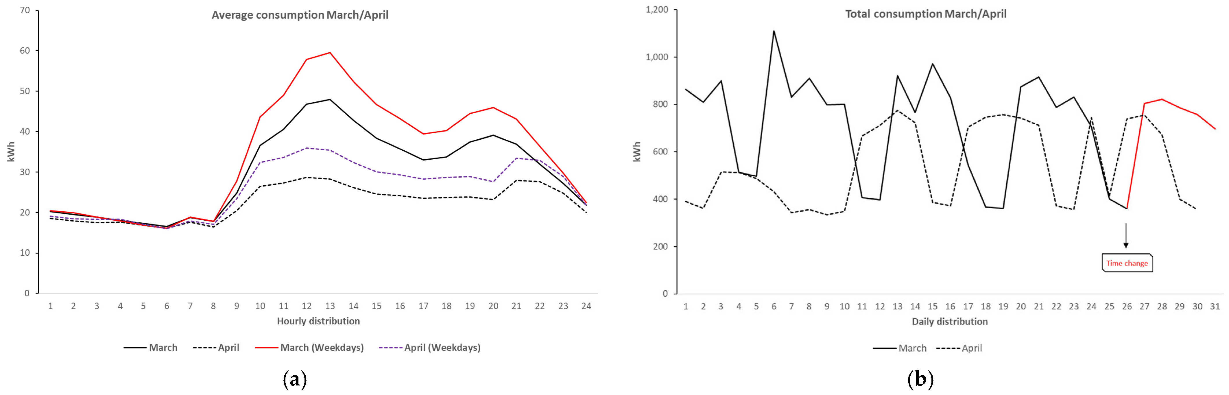
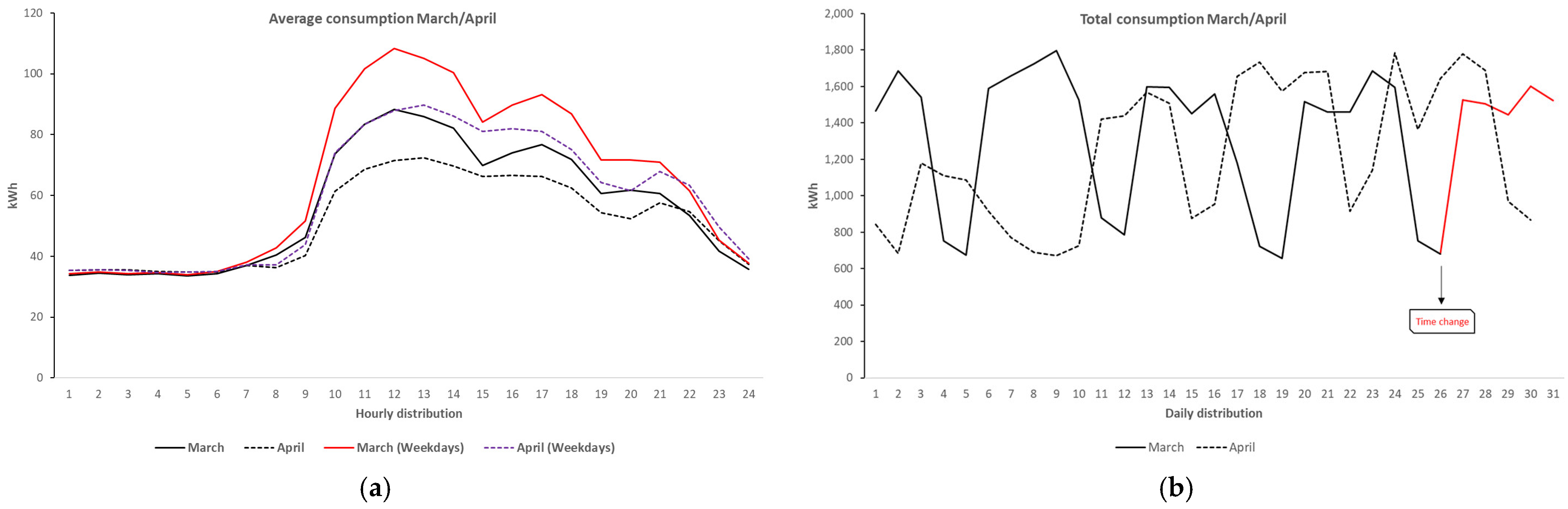
Figure 11 presents electricity consumption in March and April 2023 from both a daily (a) and hourly perspective (b). Our objective is to analyze consumption before and after the daylight saving time change. In the first graph (Figure 11a), which shows daily consumption, there is significant variation throughout the days, with well-defined peaks followed by sharp declines. March, represented by the solid line, exhibits more pronounced fluctuations, while April, indicated by the dashed line, shows a slightly more stable pattern but still with considerable variations. It is worth noting that at the beginning of April, consumption was lower due to the academic break for Easter.

The weekday consumption curve for March exhibits a pronounced and sharp peak between 10:00 AM and 12:00 PM, reaching approximately 62 kWh. This peak is substantially higher than the overall March average, which peaks at just above 50 kWh during the same timeframe. The steep rise beginning around 8:00 AM indicates a significant increase in activity, likely associated with the start of daily operations.

In contrast, the weekday consumption pattern for April also demonstrates a mid-morning increase, with the peak occurring around 12:00 PM and reaching slightly above 40 kWh. While this does represent an increase compared to the general April average, the difference is notably less pronounced than in March. The smaller variation between weekday and all-day consumption in April suggests a more consistent energy usage pattern, with reduced sensitivity to the type of day.

In the second graph (Figure 11b), which illustrates average hourly consumption, a characteristic pattern is observed throughout the day. During the early morning hours, consumption remains low and stable, starting to increase in the early morning. The peak occurs between 9 AM and 12 PM, followed by a gradual decline throughout the afternoon and evening. When comparing both months, a similar trend is observed, though slight differences in intensity may indicate variations in energy usage patterns.

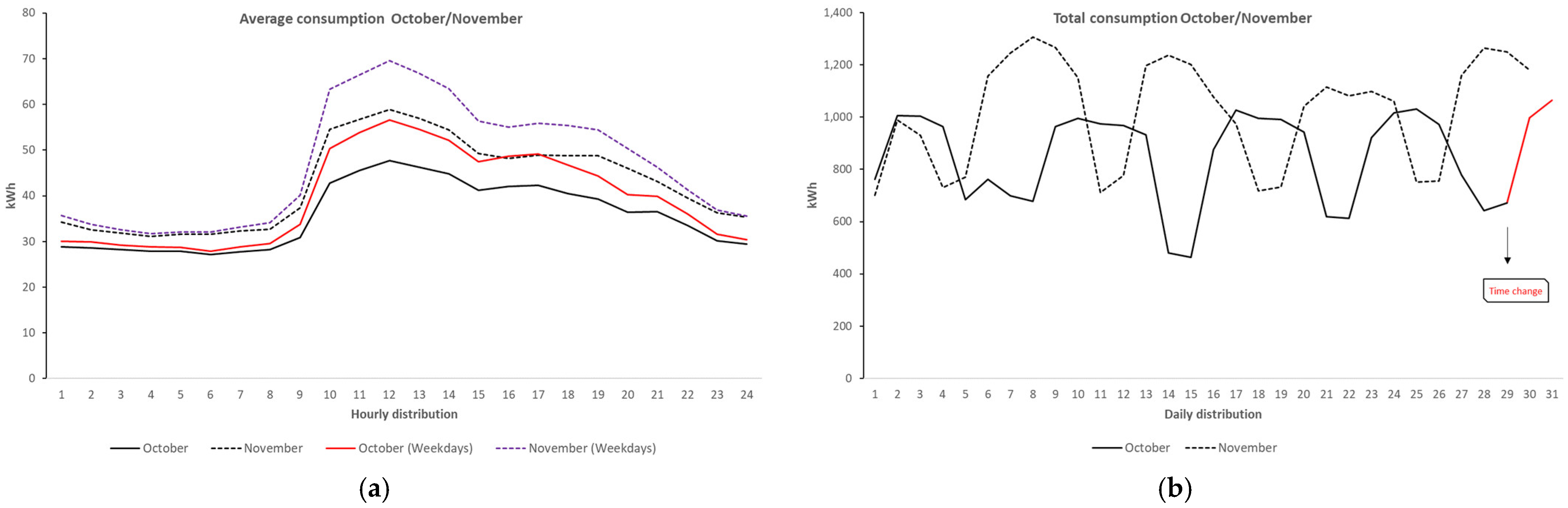
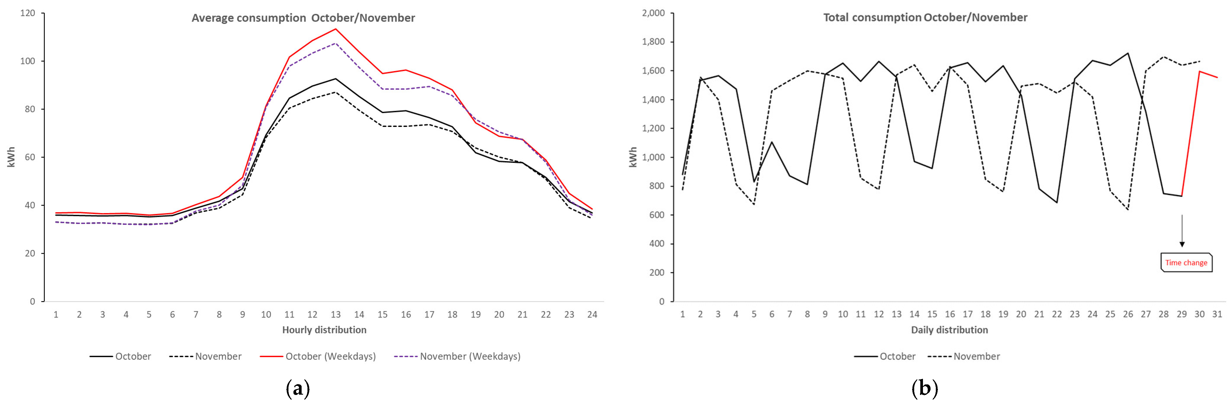
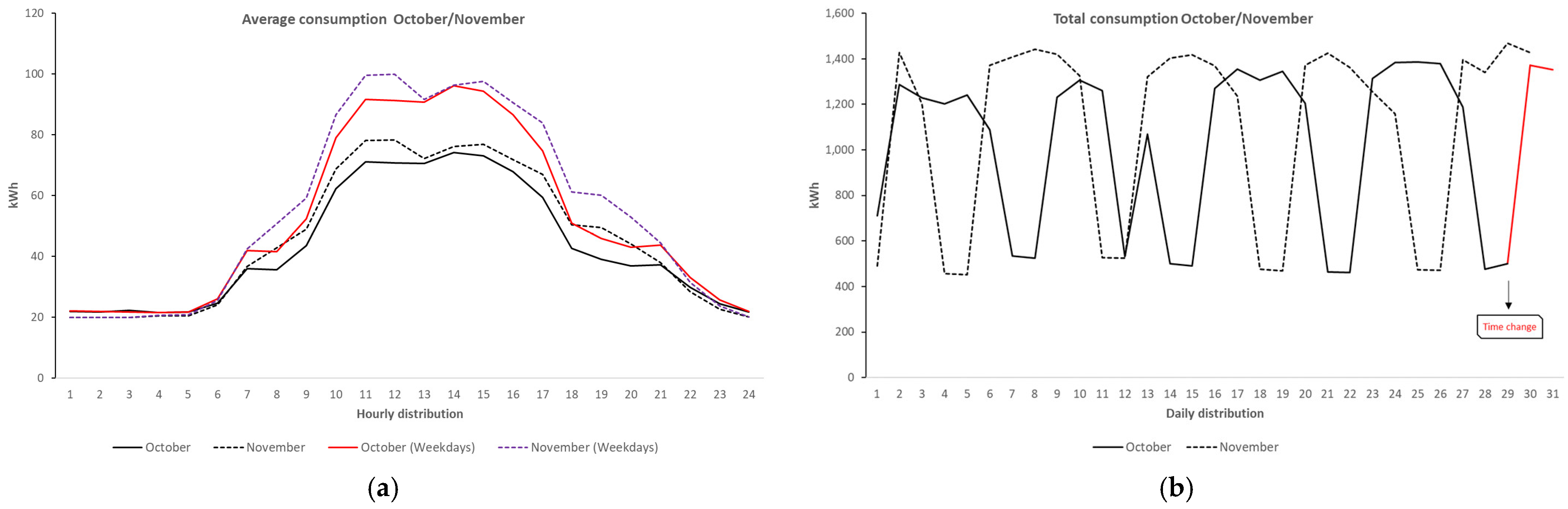
Figure 12 illustrates electricity consumption trends for October and November 2023 from both an hourly (a) and daily perspective (b). Figure 12a, representing average hourly consumption, shows a typical daily pattern, where energy usage remains low and stable during the early morning hours before rising sharply in the morning. A peak occurs between 10 AM and 1 PM, followed by a gradual decline throughout the afternoon and evening. The consumption pattern is similar for both months, but November, represented by the dotted line, shows slightly higher peak values compared to October, indicating increased energy demand.

The weekday consumption curve for October shows a clear and pronounced peak between 11:00 AM and 1:00 PM, reaching approximately 55 kWh. This value is notably higher than the overall October average, which peaks at just under 45 kWh during the same period. The steep increase beginning around 8:00 AM suggests a marked rise in activity associated with the start of the workday.

In November, the weekday pattern also demonstrates an elevated mid-morning to early afternoon consumption profile, peaking around 12:00 PM at just above 45 kWh. Compared to the general November trend, this represents a modest increase. However, the difference between weekday and all-day consumption in November is less pronounced than in October.

Figure 12b, representing daily consumption, reveals significant fluctuations throughout both months. Energy usage varies considerably from day to day, likely influenced by factors such as operational activities, weather conditions, or specific demand patterns. Notably, an anomaly is observed between 10 and 12 October. This increased consumption was caused by the use of a chiller for cooling, as temperatures exceeded 30 °C on those days. While both months exhibit similar trends, November appears slightly more stable, whereas October shows more pronounced peaks and drops. Overall, the graphs indicate a consistent pattern of energy usage, with peak demand occurring in the mid-morning to early afternoon and notable daily variations reflecting dynamic consumption behavior.

4.1.2. School of Sports and Leisure of Melgaço, Portugal (ESDLM)

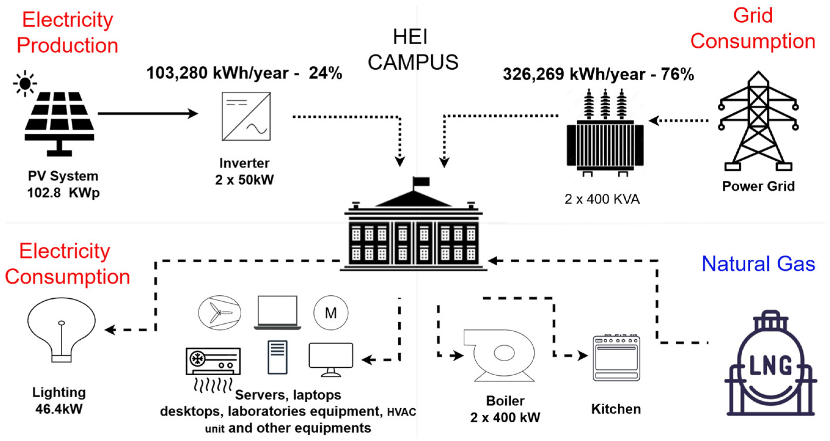
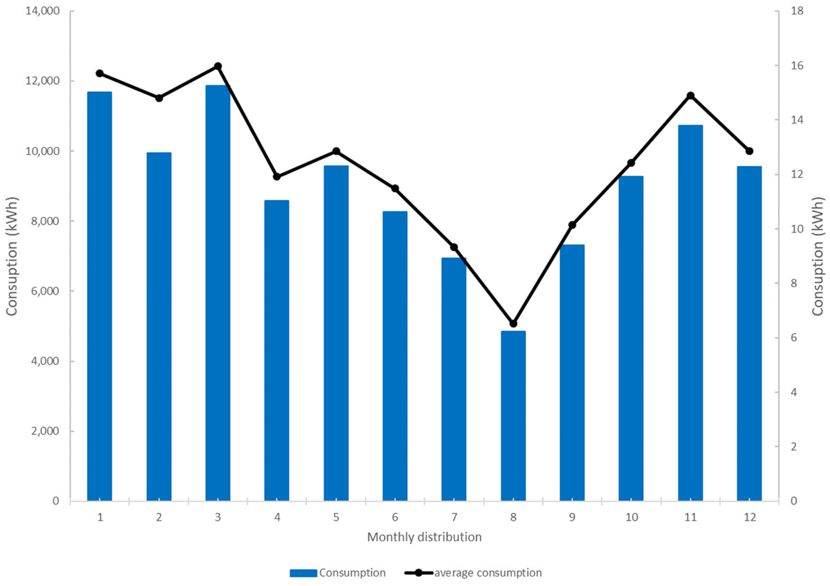
Figure 13 presents the total monthly energy consumption (in kWh) and the average hourly consumption per month for ESDLM. The blue bars represent the total consumption, while the black line indicates the average hourly consumption.

Observing the trend, energy consumption fluctuates throughout the year. The highest total consumption is recorded during the winter months, with peaks in the first and third months. In contrast, the lowest consumption occurs in August, showing a decrease of over 50%. This significant drop is directly related to the school’s summer break, as students are on vacation, and the institution remains closed for 15 days.

Similarly, the average hourly consumption follows a comparable trend. A noticeable decline is observed in February, which coincides with the exam period, when overall energy demand is lower. In December, consumption decreases compared to November, likely due to the Christmas holidays. Towards the end of the year, there is a rebound in energy usage, reflecting an increase in activity after the holiday break.

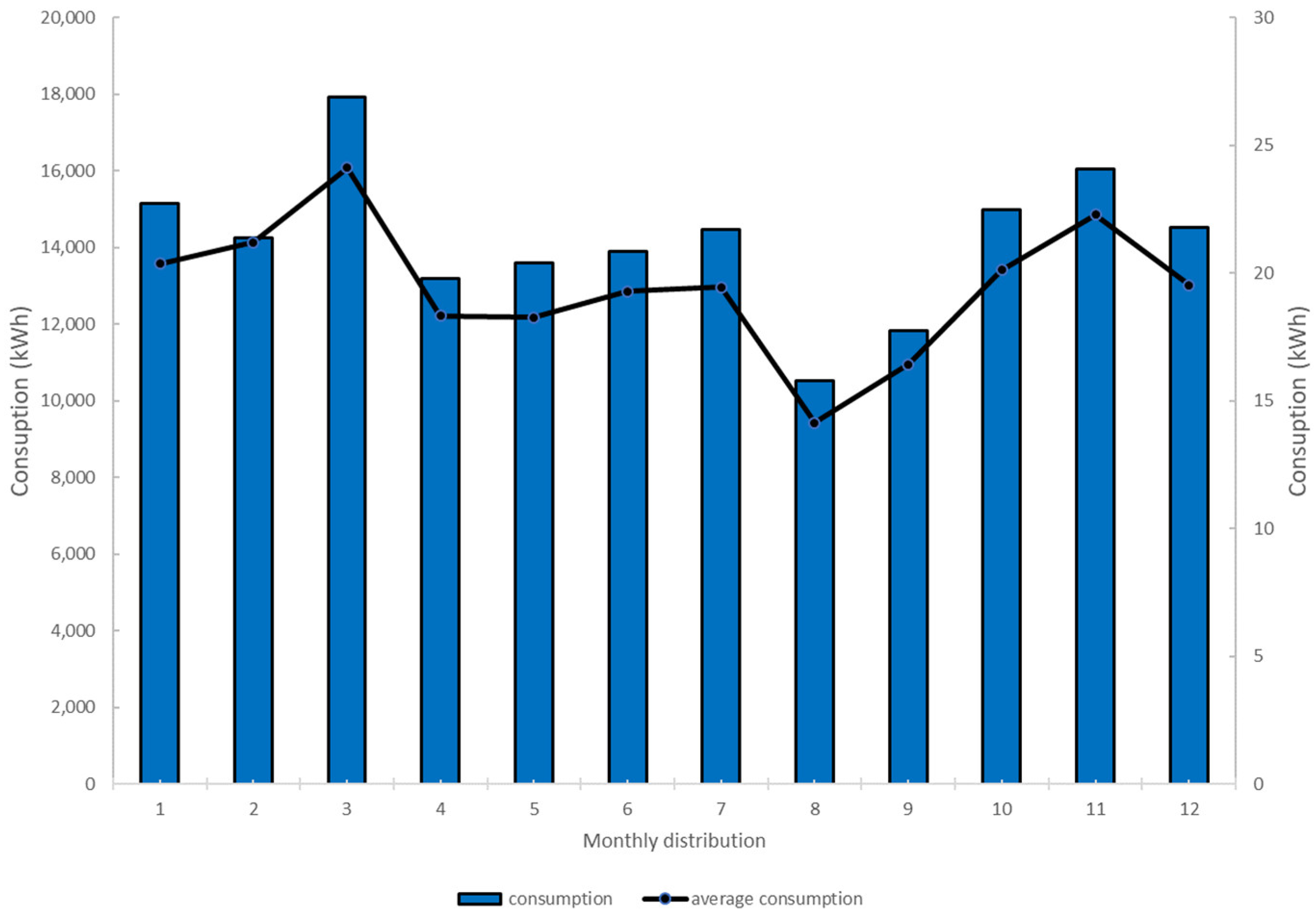
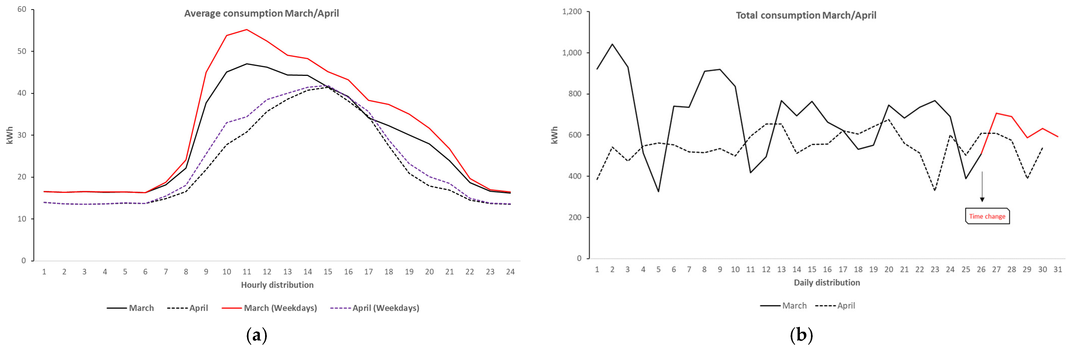
Figure 14 illustrates the average hourly consumption (left) and total daily consumption (right) for March and April 2023 at ESDLM. The hourly consumption graph represents the average electricity consumption (in kWh) during March and April, distributed throughout the hours of the day. Consumption remains low and relatively constant during the night (between 10 PM and 6 AM). From 7 AM onwards, there is a significant increase, reaching a peak between 10 AM and 12 PM. The peak in March is more pronounced, exceeding 35 kWh, whereas in April, it is slightly above 20 kWh. Additionally, April presents a more stable consumption profile between 10 AM and 2 PM, without the sharp decline observed in March. This reduction in April can be attributed to milder temperatures, leading to a lower need for heating or cooling.

The weekday consumption curve for March demonstrates a distinct and steep peak between 11:00 AM and 1:00 PM, reaching approximately 46 kWh. This is significantly higher than the overall March average, which peaks just above 35 kWh during the same time window. The sharp rise beginning around 9:00 AM suggests a rapid onset of operational or activity-related energy use, typical of a weekday working schedule.

In April, the weekday profile also shows a mid-morning increase, peaking around 12:00 PM at approximately 27 kWh. Compared to the general April curve, which peaks slightly above 21 kWh, the difference is present but more moderate.

The daily consumption graph represents the total electricity consumption (in kWh) for March and April, distributed by day. There is a cyclical pattern, with high-consumption days alternating with lower-consumption days. This behavior is influenced by the academic schedule, as classes take place from Monday to Friday, while on weekends, consumption remains low and constant. At the beginning of April, a noticeable drop in consumption is observed, which coincides with the Easter holiday break, when academic activities are paused.

Overall, the data highlight clear patterns influenced by school schedules. The peak consumption during the day aligns with academic hours, while the variations between March and April suggest seasonal or operational factors affecting energy demand.

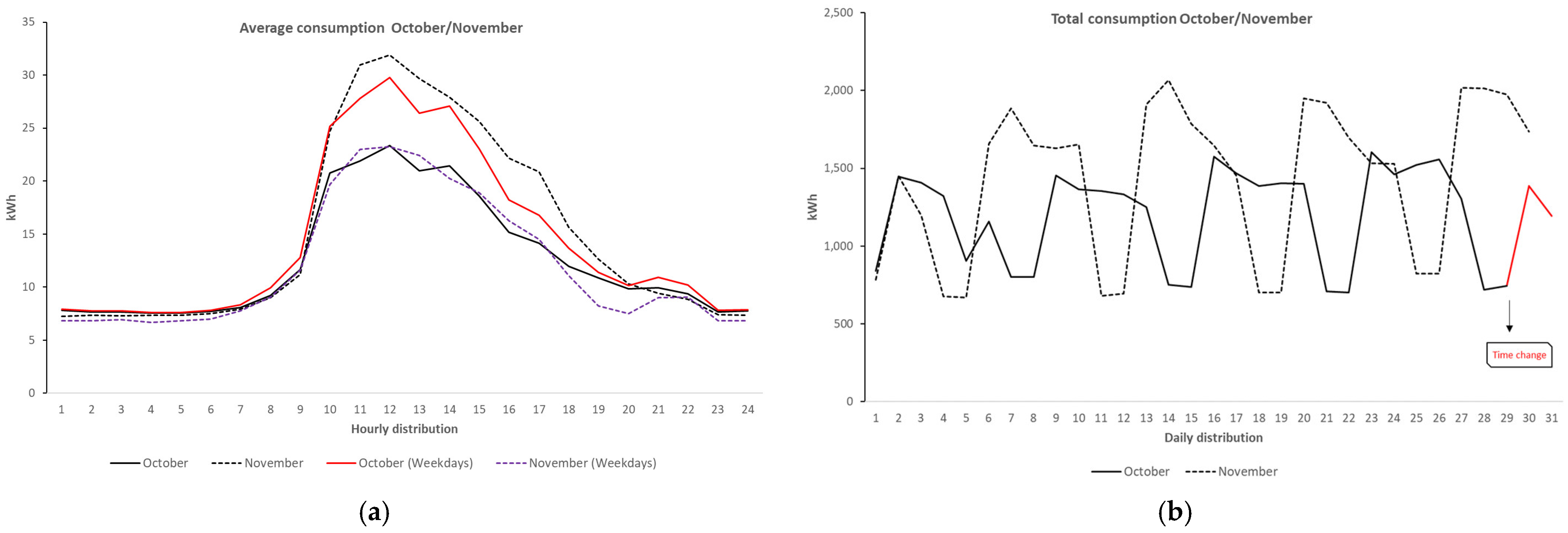
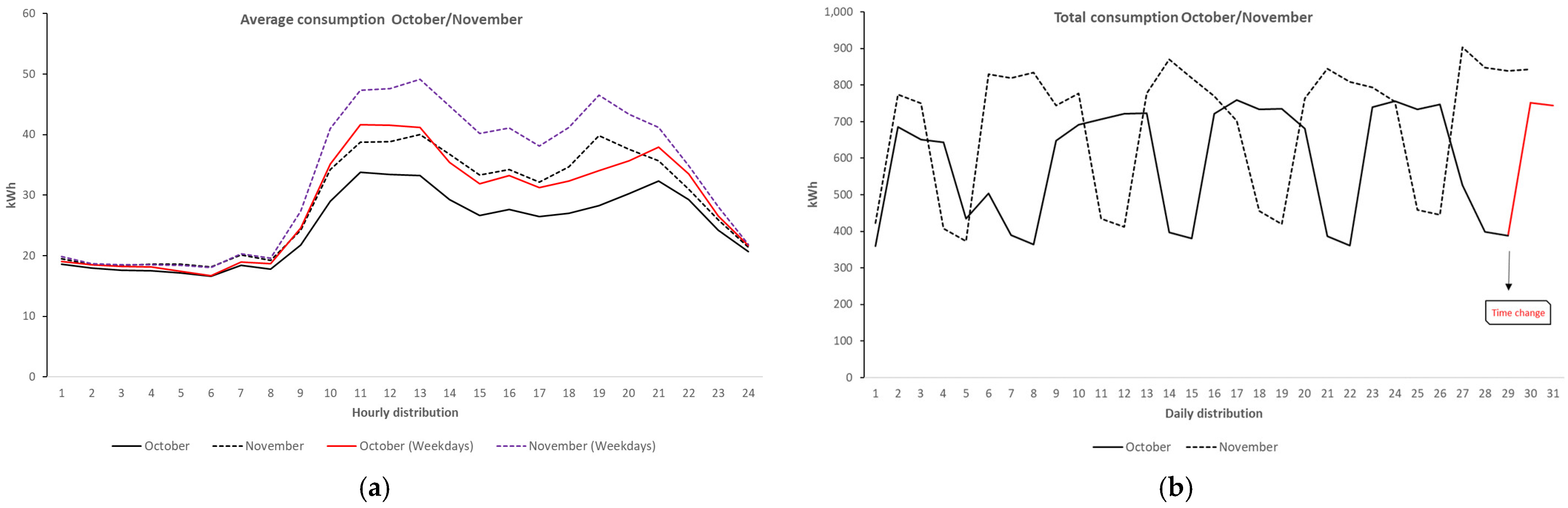
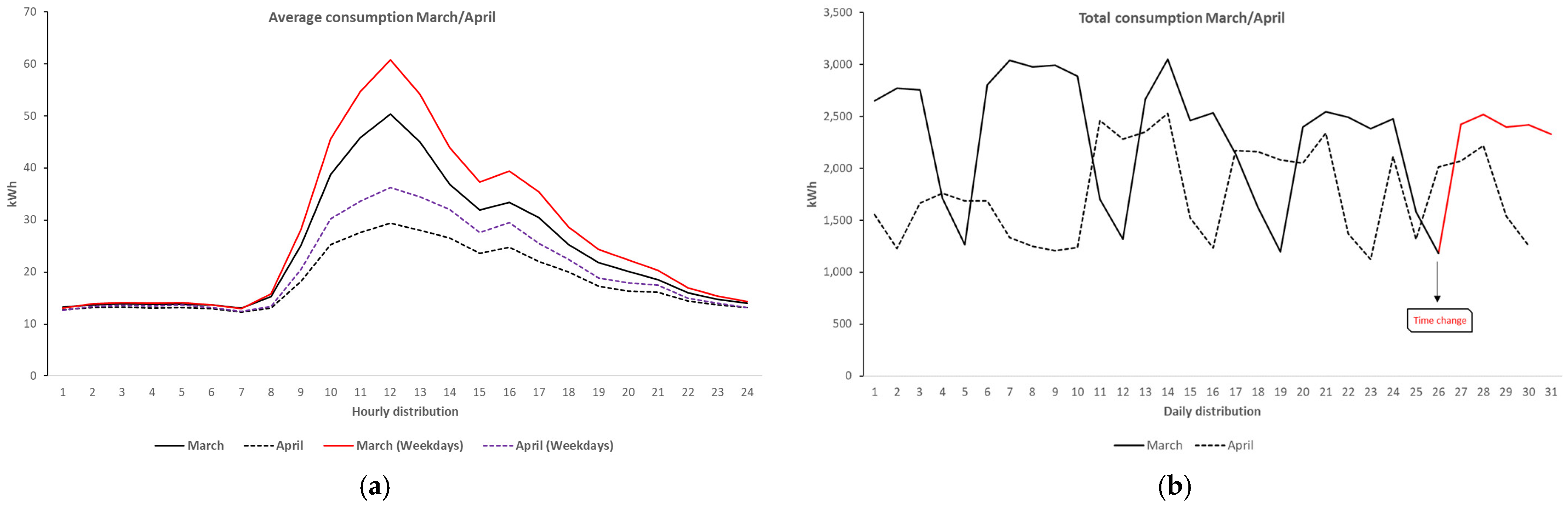
In Figure 15, the first graph (a) illustrates the average hourly energy consumption for October and November 2023, showing a clear peak between 10:00 and 14:00, with November reaching a higher peak than October. As expected, November’s consumption is higher than October’s; however, the facility reports stable consumption between 23:00 and 08:00 in both months. Additionally, in the hourly distribution graph, it is possible to observe low consumption on 5 October, which corresponds with a national holiday.

The weekday consumption profile for October exhibits a sharp increase starting around 9:00 AM, reaching a peak between 11:00 AM and 12:00 PM at approximately 30 kWh. This is notably higher than the overall October average, which peaks during the same timeframe but at a lower value of around 23 kWh.

In contrast, the November profile shows an even more pronounced surge in average consumption, peaking at roughly 33 kWh between 11:00 AM and 12:00 PM. Interestingly, the weekday-specific curve for November peaks at a lower value, just under 24 kWh.

The second graph (b) presents the total daily consumption, revealing a cyclical pattern likely related to weekly variations, with lower consumption on certain days, possibly weekends. This cyclical pattern remains consistent during the winter months. November generally exhibits higher consumption than October, with more pronounced peaks, indicating increased energy demand. Overall, both graphs suggest that energy usage in November was higher than in October, with significant variations in daily and hourly consumption patterns, likely influenced by operational or seasonal factors.

4.1.3. Agrarian School of Ponte de Lima, Portugal (ESAPL)

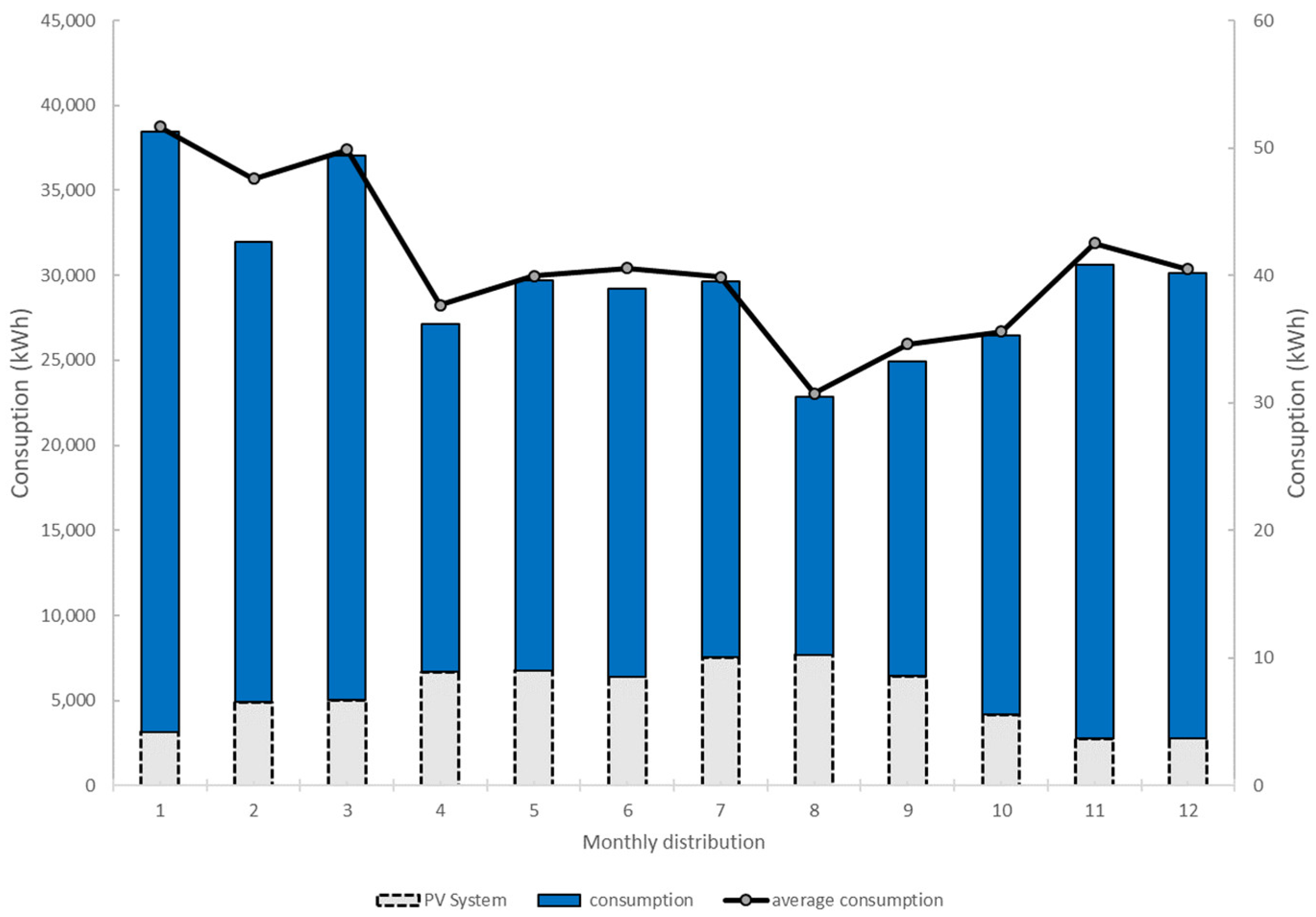
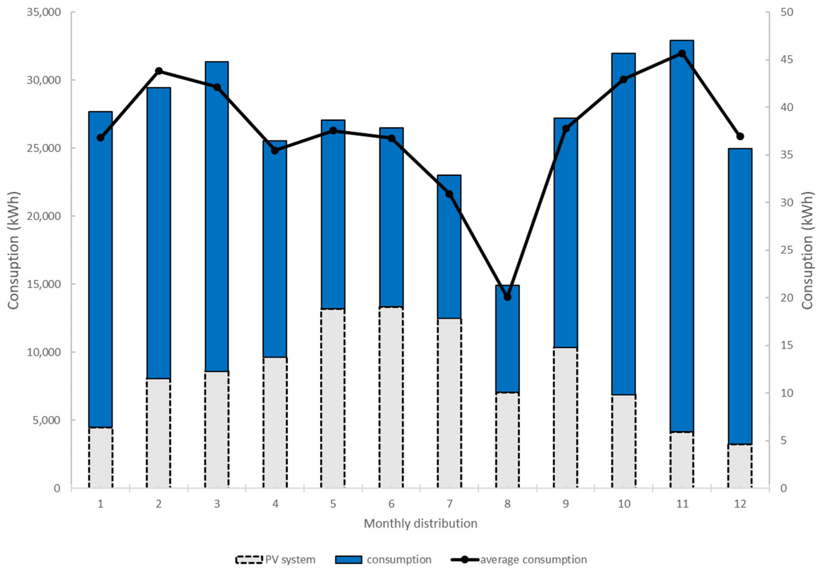
The graph presented in Figure 16 illustrates the total monthly electricity consumption and average hourly consumption per month for ESAPL. The blue bars represent the total monthly consumption (kWh), while the black line indicates the average hourly consumption (kWh). Additionally, the contribution from photovoltaic energy is depicted with a dashed line.

This installation is different, as it incorporates a photovoltaic system, which contributes to the total energy supply. However, as observed in the graph, the photovoltaic contribution remains relatively low compared to total consumption, indicating that a substantial portion of the energy demand is still met by external sources.

The data reveal seasonal variations in energy consumption, with higher values recorded in the first quarter of the year (January to March), peaking above 35,000 kWh. A sharp decline is observed in April, followed by a period of relative stability between May and July. The lowest total consumption is noted in August, after which there is a gradual recovery, leading to another peak in November and December. The average hourly consumption follows a similar pattern, with higher values during the beginning and end of the year and a decline in the middle months.

It is important to consider that this campus consists of both an academic building and a student residence, which may influence the observed consumption trends. The academic building’s energy demand is likely driven by class schedules, laboratory activities, and administrative operations, whereas the student residence exhibits a more continuous consumption profile, with possible variations during academic breaks and holiday periods. This distinction may help explain the reduction in consumption during August, when academic activities are minimal and student occupancy is lower.

The presence of the photovoltaic system, despite its relatively small contribution, suggests potential for greater renewable energy integration. Future research could investigate ways to optimize photovoltaic energy use, such as storage solutions or demand-side management strategies, to enhance self-sufficiency and sustainability in ESAPL’s energy consumption.

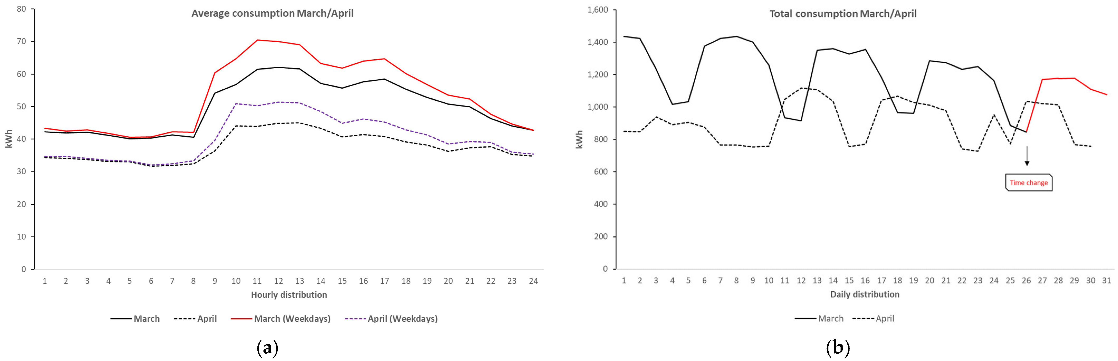
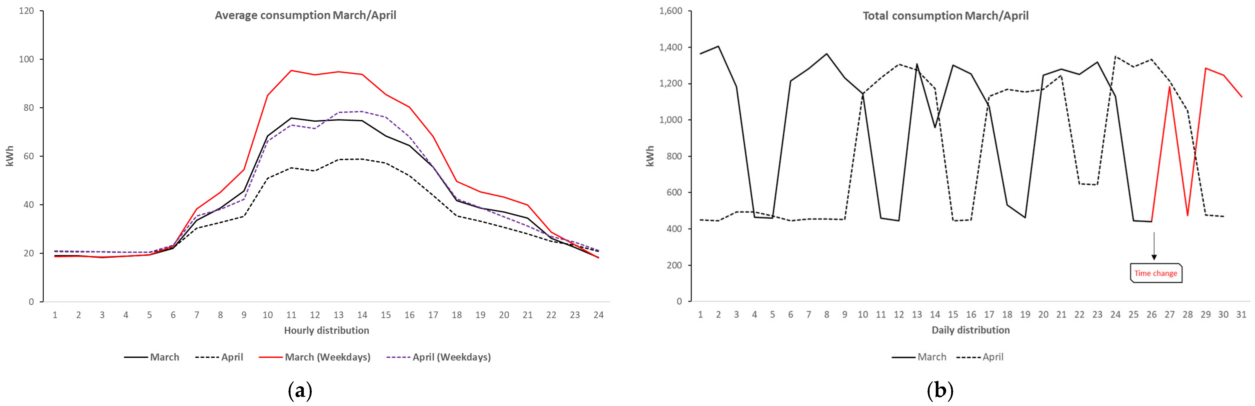
The graphs presented in Figure 17 illustrate the average hourly consumption (a) and total daily consumption (b) for March and April 2023 at ESAPL. The solid line represents March, while the dashed line corresponds to April.

In Figure 17a, the average hourly consumption in March is consistently higher than in April throughout the day. A notable increase in consumption begins at 8:00 AM, peaking between 10:00 AM and 2:00 PM, followed by another rise during dinner hours and a slower decline at night. This trend suggests that energy demand is strongly influenced by the academic building’s activities during the day and by the student residence at night. Additionally, the canteen operations at lunch and dinner contribute to peak consumption periods. April follows a similar pattern but with lower absolute values, potentially due to reduced academic activities or lower student occupancy during holiday periods.

The weekday consumption profile for March exhibits a pronounced peak between 10:00 AM and 12:00 PM, reaching nearly 70 kWh. This is noticeably higher than the general March average (black line), which peaks just above 60 kWh during the same period. The rapid increase beginning around 9:00 AM highlights the onset of intensive weekday operations.

For April, the weekday pattern also demonstrates an increase during the mid-morning to early afternoon period, peaking at approximately 50 kWh around 11:00 AM. Compared to the overall April curve, which peaks closer to 45 kWh, the difference is evident but less substantial than in March.

Figure 17b further supports this observation, showing that the total daily consumption in March is consistently higher than in April. Additionally, March exhibits greater daily consumption variability, with peaks exceeding 1400 kWh on certain days, whereas April displays a more stable curve, with lower fluctuations and values generally below 1200 kWh. A significant drop in consumption is observed on 25 April, corresponding to a national holiday, as well as during the Easter break, when academic activities and the student presence on campus are likely reduced.

These findings align with the seasonal consumption trends identified in Figure 17, where April showed a reduction in total energy demand compared to March. The decrease in consumption may be attributed to changes in campus occupancy, academic holiday periods, or operational adjustments.

Given that this facility integrates a photovoltaic system, a more detailed analysis could investigate the relationship between solar generation and hourly consumption, as well as potential strategies to optimize self-consumption of renewable energy. Approaches such as load management and energy storage could help reduce reliance on the grid and enhance the overall energy efficiency of the installation.

Figure 18 illustrates the average hourly consumption (a) and total daily consumption (b) for October and November 2023 at ESAPL. The first graph shows the hourly distribution of energy consumption, highlighting a noticeable increase in demand during daytime hours, particularly between 10:00 and 15:00. In November, energy usage appears consistently higher than in October, with a more pronounced peak around midday, indicating seasonal variations or increased activity during this period.

The weekday consumption curve for November displays a distinct and sharp increase starting around 9:00 AM, reaching a peak of nearly 70 kWh by midday. This is significantly higher than the general average for November, which remains below 60 kWh during the same period.

October’s weekday consumption also demonstrates a mid-morning increase, though to a lesser extent. The peak reaches just under 60 kWh, compared to approximately 50 kWh for the overall October average. Despite the visible weekday effect, the differential between weekday and overall values in October is less pronounced than in November.

The second graph presents the total daily consumption across both months. A recurrent pattern can be observed, with alternating peaks and troughs that suggest cyclical consumption trends. November exhibits higher overall energy demand, with more pronounced fluctuations compared to October, likely influenced by operational or environmental factors. These results provide insights into energy consumption behaviors, which can be useful for optimizing energy efficiency and planning future energy supply strategies.

4.1.4. School of Education Sciences of Viana do Castelo, Portugal (ESEVC)

Figure 19 illustrates the total monthly energy consumption and the average hourly consumption per month for ESEVC. The bar chart represents the total energy consumption (kWh) for each month, while the line graph indicates the corresponding average hourly consumption. A clear seasonal trend is observed, with higher consumption levels in the winter months (January, February, and December) and a decline during the summer period, particularly in July and August. This variation is likely influenced by seasonal factors, such as heating demands in winter and reduced activity during summer vacation months. Notably, the school closes for two weeks in August, which contributes to the significant drop in energy consumption during this period. Additionally, a strong correlation between total monthly consumption and average hourly consumption is evident, as the trends in both datasets follow a similar pattern. The peaks in consumption during the colder months suggest a significant dependency on climate-related energy usage, which should be considered for energy efficiency and sustainability planning.

Figure 20 presents the average hourly consumption (a) and total daily consumption (b) for March and April 2023 at ESEVC. The first graph demonstrates the hourly distribution of energy consumption, showing a clear peak in March between 10:00 and 14:00, which is more pronounced than in April. In contrast, April exhibits a more stable consumption pattern throughout the day, with lower overall energy usage compared to March. This suggests variations in operational activity, possibly influenced by differences in school schedules or external factors such as weather conditions.

The weekday consumption profile for March reveals a marked and rapid increase beginning around 9:00 AM, reaching a peak of approximately 60 kWh by midday. This value significantly exceeds the general March average, which peaks near 47 kWh in the same timeframe. In contrast, the weekday profile for April also shows a mid-morning increase, albeit more moderate, peaking at around 35 kWh.

The second graph highlights daily energy consumption trends for both months. March shows higher and more fluctuating consumption levels, whereas April follows a more regular pattern with periodic decreases, likely corresponding to weekends or holidays. These variations may reflect differences in academic schedules, operational demand, or external influences. The data indicate that March experiences higher overall energy demand, reinforcing the need to analyze the impact of academic activities and external conditions on energy consumption patterns.

On campus, they have an academic residence, classroom building, and football field. The graph clearly indicates the period during which the lighting of the football field is used, which is combined with the period of preparation of meals for dinner. The reduction in consumption during the Easter holiday period is noticeable.

The analysis of Figure 21 reveals significant patterns in both hourly and daily electricity consumption for October and November 2023 at ESEVC. The first graph (a), which depicts the average hourly consumption, shows a clear increase in demand starting at approximately 7:00, peaking between 10:00 and 12:00, and maintaining relatively high levels throughout the afternoon before gradually declining in the evening. Notably, November exhibits slightly higher consumption levels compared to October, particularly during peak hours, suggesting either increased activity or colder temperatures requiring additional energy use. The observed peaks likely correspond to meal production times and the lighting of the football field, contributing to higher consumption during specific periods.

The weekday consumption profile for November displays a marked increase beginning around 9:00 AM, culminating in a pronounced double peak—first between 11:00 AM and 12:00 PM, and again between 7:00 PM and 8:00 PM—both reaching values around 50 kWh. The overall November profile follows a similar trend but with slightly lower intensity, peaking at approximately 45 kWh.

October, in comparison, shows a more moderate pattern. The weekday profile increases steadily from 9:00 AM and plateaus around 11:00 AM, maintaining a level of approximately 40 kWh throughout the afternoon. The overall October curve is consistently lower, peaking just above 35 kWh.

The second graph (b), illustrating total daily consumption, highlights considerable fluctuations across both months. A recurring pattern emerges, where consumption tends to be higher on certain days, likely corresponding to weekdays, while a marked drop is observed on other days, possibly weekends. The impact of the October holiday is also visible, resulting in a significant decrease in consumption on that specific day. November generally shows higher total daily consumption than October, reinforcing the trend observed in the hourly data. The variations between consecutive days suggest dynamic energy usage, potentially influenced by operational schedules, climatic conditions, or institutional activities. These findings indicate the need for further investigation into specific factors influencing consumption patterns, which could be essential for optimizing energy efficiency and implementing demand-side management strategies.

4.1.5. School of Health Sciences of Viana do Castelo, Portugal (ESSVC)

Figure 22 illustrates the total monthly consumption and the average hourly consumption per month at ESEVC. The data reveal a clear seasonal trend, with the highest total consumption observed in the winter months (January, February, November, and December) and the lowest in August. This pattern likely reflects variations in institutional activity, with reduced operations during summer months leading to lower energy demand. Notably, the institution closes for 15 days in August, which significantly contributes to the sharp drop in consumption during that month.

The average hourly consumption, represented by the black line, follows a similar trend, decreasing steadily from January to August before increasing again towards the end of the year. The lowest values occur in August, reflecting the partial closure of the institution. From September onward, both total and average hourly consumption increase, reaching their peak in December, possibly due to extended heating and lighting requirements during colder months.

The PV system’s contribution, shown in the dashed bars, remains relatively constant throughout the year but only covers a fraction of the total energy demand. This suggests that while photovoltaic generation provides some energy savings, additional measures may be required to further optimize consumption, particularly during high-demand months.

Figure 23 presents the average hourly consumption (a) and total daily consumption (b) for March and April 2023 at ESEVC. The first graph (a) shows a clear difference in energy usage patterns between the two months. In March, there is a sharp increase in consumption starting around 7:00, reaching a peak between 9:00 and 12:00, and maintaining high levels until approximately 15:00 before gradually decreasing in the evening. In contrast, April exhibits a lower and more stable consumption pattern throughout the day, with a peak occurring slightly later and at a reduced magnitude compared to March. This suggests that March may have had higher institutional activity or additional energy demands during morning hours.

March (Weekdays) shows a significantly sharper peak between 9 AM and 12 PM, reaching nearly 60 kWh, compared to the general March average, which peaks just above 50 kWh. April (Weekdays) also shows a noticeable increase in the mid-morning to early afternoon period compared to the overall April data, though the differences are smaller than in March.

The second graph (b) illustrates total daily consumption, highlighting significant fluctuations in March, while April presents a more stable daily profile with lower overall consumption. The peaks in March indicate days with considerably higher energy demand, possibly due to specific events, increased occupancy, or operational factors. In contrast, April maintains a more uniform consumption pattern, suggesting reduced variability in institutional activities.

These results indicate that March had higher energy demands, particularly in the morning, whereas April displayed a more balanced and lower consumption trend. This Institution has only classes and does not serve dinners.

Figure 24 presents the average hourly consumption (a) and total daily consumption (b) for October and November 2023 at ESSVC. The left graph (a) illustrates the hourly energy consumption pattern, showing a marked increase in demand starting around 7:00 AM, peaking between 10:00 AM and 12:00 PM, and then gradually declining throughout the afternoon and evening. Notably, November exhibits slightly higher consumption during peak hours compared to October, suggesting a seasonal effect or increased activity during this period.

The weekday consumption curve for November reveals a sharp and early morning increase starting around 7:00 AM, peaking steeply between 10:00 AM and 11:00 AM at approximately 47 kWh. This peak significantly exceeds the overall November average, which reaches a lower maximum of around 38 kWh during the same time window.

In comparison, October presents a more moderate profile. The weekday curve shows a rapid increase beginning after 8:00 AM, peaking between 11:00 AM and 12:00 PM at just above 34 kWh. This is higher than the overall October curve, which plateaus at approximately 30 kWh during midday.

The right graph (b) displays the total daily energy consumption for both months. The data reveal significant day-to-day fluctuations, with peaks observed around the middle and end of the month, particularly in November. This variability may be attributed to operational changes, external temperature influences, or specific events that led to increased energy demand. Additionally, the general trend suggests that November had higher overall consumption than October, aligning with the hourly distribution analysis.

4.1.6. School of Technology and Management of Viana do Castelo, Portugal (ESTGVC)

Figure 25 illustrates the total monthly energy consumption and the average hourly consumption per month for ESTGVC, comparing data from March and April. The left graph (a) displays the average hourly energy consumption, showing a distinct increase in demand from early morning onwards, peaking between 9:00 AM and 12:00 PM. The consumption then remains relatively stable in the afternoon before gradually declining in the evening. Notably, March exhibits higher peak consumption levels compared to April, suggesting a possible decrease in energy demand during the latter month. This variation may be linked to external factors such as academic schedules, temperature differences, or operational adjustments within the facility. The right graph (b) presents the total daily energy consumption for both months, revealing significant fluctuations in demand across individual days. March shows higher peaks on several days compared to April, reinforcing the trend observed in the hourly distribution. The variability observed in both months suggests that energy consumption is influenced by specific operational or external conditions, leading to periodic spikes in demand. It is also important to note that ESTGVC closes for 15 days in August, which likely results in a significant reduction in energy consumption during that period.

The analysis of Figure 26, which presents the average hourly consumption (a) and total daily consumption (b) for March and April 2023 at ESTGVC, reveals significant variations in energy usage patterns. The first graph (a) indicates a marked increase in electricity demand during working hours, particularly from 8 AM to 2 PM, followed by a gradual decline in the evening. This pattern aligns with the operational schedule of the institution, which is the largest school within IPVC, hosting daytime and evening classes and providing lunch and dinner services. The higher consumption in March compared to April suggests seasonal or academic calendar influences, possibly linked to variations in class schedules or occupancy levels.

The weekday consumption profile for March reveals a pronounced and rapid increase beginning around 9:00 AM, culminating in a distinct peak at approximately 11:00 AM, reaching just above 105 kWh. This is substantially higher than the overall March average, which peaks at around 85 kWh during the same timeframe.

In April, the weekday curve also demonstrates a steep rise starting at 9:00 AM, with a peak of roughly 90 kWh around 12:00 PM. This contrasts with the overall April profile, which peaks lower, around 75 kWh.

The second graph (b), illustrating total daily consumption, presents a highly fluctuating pattern, reflecting variations in daily energy needs. The significant peaks and troughs suggest differences in activity levels on specific days, potentially influenced by the presence of exams, special events, or variations in student and staff attendance. March generally exhibits higher overall consumption than April, reinforcing the possibility of reduced activities or occupancy changes.

The analysis of Figure 27, which presents the average hourly consumption (a) and total daily consumption (b) for October and November 2023 at ESTGVC, highlights significant variations in energy usage patterns influenced by specific events. In graph (a), the hourly consumption follows a similar trend for both months, with a pronounced increase from 8 AM, peaking around noon, and gradually declining in the evening. However, October exhibits slightly higher values, which can be attributed to various organized events during this period, including the Sustainable Campus Conference, student festivities during nighttime hours, and other academic activities.

The weekday consumption profile for October shows a sharp and rapid increase beginning around 9:00 AM, peaking near 1:00 PM at just under 115 kWh. This level is significantly higher than the overall October average, which reaches a lower peak of approximately 95 kWh during the same period.

In November, the weekday profile also exhibits a marked rise starting around 9:00 AM, with a peak of about 105 kWh around 1:00 PM. This contrasts with the overall November average, which peaks at around 90 kWh.

In graph (b), daily consumption shows a fluctuating pattern, with October displaying higher overall consumption than November. This trend is unique among the studied entities, as all others exhibited higher energy usage in November. The increased activity in October explains this deviation, reinforcing the impact of events on electricity demand. Additionally, the significant drop in consumption observed on November 5 clearly marks a public holiday, further confirming the correlation between academic operations and energy usage patterns.

4.1.7. School of Mines and Energy, University of Vigo, Spain (UVEM)

The analysis of Figure 28, which presents the total monthly consumption and average hourly consumption per month for UVEM, reveals distinct seasonal variations in energy demand. The blue bars indicate total monthly consumption, while the black line represents the average hourly consumption. The data show higher energy consumption during the winter months (January, February, November, and December), with peaks in February and November, likely due to increased heating demands and operational intensity during these periods. A notable decline in energy consumption is observed during the summer months, particularly in August, which corresponds to a period of reduced activity due to academic breaks or lower occupancy levels. This trend is further supported by the simultaneous reduction in both total and average hourly consumption. The presence of a photovoltaic (PV) system, represented by the dashed bars, highlights the contribution of renewable energy to overall consumption, which remains relatively stable across the months.

The data underscore the importance of seasonal influences on energy consumption, demonstrating how institutional activity levels and climatic conditions impact overall demand. Understanding these variations is crucial for implementing effective energy management strategies, optimizing PV system utilization, and improving energy efficiency in educational and research facilities.

Figure 29 presents the average hourly consumption (a) and total daily consumption (b) for March and April 2023 at UVEM. The first graph shows a clear diurnal pattern, with energy consumption increasing sharply from around 6 to 7 AM, reaching its peak between 10 AM and 3 PM, and then gradually decreasing after 5 PM. This trend suggests a strong correlation with human activity, likely corresponding to operational hours. The comparison between March and April indicates similar overall behavior, although April exhibits slightly lower peak values, which could be attributed to seasonal variations, changes in operational schedules, or energy efficiency measures.

The weekday consumption profile for March exhibits a rapid increase starting around 7:00 AM, reaching a sharp and sustained peak of approximately 95–100 kWh between 10:00 AM and 1:00 PM. This is significantly higher than the overall March average, which peaks lower, at around 75 kWh during the same period.

In April, the weekday profile also shows a notable rise beginning at 7:00 AM, peaking around 11:00 AM to 12:00 PM at roughly 80 kWh. This contrasts with the overall April average, which peaks at approximately 60 kWh.

The second graph highlights the daily energy consumption, revealing significant fluctuations, particularly in March, where sharp peaks and drops suggest intermittent high-consumption events or irregular operational patterns. April, in contrast, presents a more stable trend with fewer extreme variations, indicating a potentially different load management approach or altered usage patterns. Despite these variations, the overall energy consumption for both months appears comparable. These trends provide valuable insights into energy usage at UVEM, emphasizing the importance of understanding load dynamics for potential optimization. Further analysis could explore external influencing factors such as temperature, occupancy, or operational constraints to identify strategies for improved energy efficiency and demand-side management.

Figure 30 presents the average hourly consumption (a) and total daily consumption (b) for October and November 2023 at UVEM. The first graph demonstrates a well-defined diurnal pattern, with energy consumption remaining low during early morning hours, followed by a sharp increase starting around 6–7 AM. The peak consumption occurs between 10 AM and 3 PM, after which there is a gradual decline. This trend suggests that energy use is primarily driven by daytime activities, likely associated with operational hours. The curves for October and November exhibit similar behavior, with November showing slightly higher values during peak hours, possibly due to increased demand or variations in environmental conditions affecting energy usage.

The weekday consumption profile for October reveals a pronounced and rapid increase starting at around 6:00 AM, with a sharp climb between 8:00 and 10:00 AM, reaching a peak of approximately 95 kWh by 12:00 PM. This value is noticeably higher than the overall October average, which peaks more modestly at around 75 kWh.

In November, the weekday profile shows an even steeper early morning ramp-up, beginning around 6:00 AM and peaking between 11:00 AM and 1:00 PM at just above 100 kWh. This contrasts with the overall November average, which peaks lower, around 80 kWh.

The second graph depicts daily energy consumption and reveals a periodic pattern with alternating high and low values. This fluctuation suggests a structured operational cycle, potentially influenced by weekdays and weekends or scheduled energy-intensive activities. The overall magnitude of consumption appears relatively stable across both months, though November exhibits a more consistent pattern with fewer extreme drops compared to October. This stability may indicate improved load distribution or fewer disruptions in energy usage.

4.1.8. Analysis of Energy Consumption with a Comparison to Sunlight Hours

To determine the hours of sunlight, sunrise, and sunset, times for the year 2023 were collected based on the region’s coordinates (sourced from https://www.sunrise-and-sunset.com, accessed on 19 December 2024). This information was then organized by month, and the monthly averages for sunrise and sunset times were calculated. The same method was applied to compute the average day length for each month.

Table 3. Variation in day length and monthly energy consumption in HEIs.

Month	Sunrise Time	Sunset Time	Day Length	ESCEV (kWh)	ESEVC (kWh)	ESAPL (kWh)	ESSVC (kWh)	ESTGVC(kWh)	ESDLM (kWh)	UVEM (kWh)
Jan	07:58	17:28	09:30	15,148	21,693	38,440	21,682	37,643	11,674	27,692
Feb	07:30	18:06	10:36	14,254	17,506	31,966	20,113	32,260	9,954	29,436
Mar	06:47	18:39	11:52	17,913	22,329	37,030	21,105	41,601	11,871	31,335
Apr	06:55	20:13	13:18	13,198	16,178	27,107	16,418	36,906	8,581	25,527
May	06:16	20:44	14:28	13,592	18,188	29,720	17,414	40,782	9,564	27,036
Jun	06:01	21:08	15:07	13,889	16,929	29,207	17,187	37,754	8,266	26,467
Jul	06:14	21:05	14:51	14,467	14,261	29,661	14,646	33,015	6,939	22,992
Aug	06:44	20:32	13:48	10,524	11,456	22,850	9,260	22,863	4,849	14,933
Sep	07:15	19:42	12:27	11,828	13,724	24,902	10,745	32,720	7,305	27,178
Oct	07:46	18:52	11:06	14,990	18,459	26,487	13,056	40,802	9,266	31,954
Nov	07:23	17:13	09:50	16,048	20,691	30,628	15,410	39,381	10,730	32,890
Dec	07:53	17:04	09:11	14,527	19,199	30,115	21,926	33,823	9,551	24,962

presents the variation in day length and monthly energy consumption in HEIs, considering a set of variables associated with sunrise and sunset times, day length, and the monthly energy consumption of the Higher Education Institutions (HEIs) under study. As expected, day length follows a seasonal pattern, being shorter in winter months—approximately 9 h in December and January—and longer during the summer, reaching around 15 h in June. Variations in energy consumption throughout the year reveal significant fluctuations, resulting from both academic dynamics, marked by the presence or absence of teaching activities, and climatic factors, particularly ambient temperature. In general, energy consumption increases during colder months, which can be attributed to the intensified use of heating systems in university facilities. A sharp decrease in consumption is observed in August, a period corresponding to the academic break and a high incidence of staff vacations. On the other hand, an increase in energy consumption is recorded in March in most institutions, reflecting the resumption of academic activities after the break for exams at the end of January and throughout February. In this context, April and August represent evident transition periods in the energy consumption pattern, reflecting the influence of holiday periods and changes in the dynamics of academic activities. These results highlight the importance of considering seasonality and the organization of the academic calendar in the management of energy efficiency in higher education institutions.

Table 4. Monthly percentage variation in energy consumption in HEIs.

Month	ESCE (%)	ESE (%)	ESA (%)	ESS (%)	ESTG (%)	ESDL (%)	VIGO (%)	Average (%)
Jan	4%	11%	22%	−1%	10%	18%	10%	11%
Feb	−6%	−24%	−20%	−8%	−17%	−17%	6%	−12%
Mar	20%	22%	14%	5%	22%	16%	6%	15%
Apr	−36%	−38%	−37%	−29%	−13%	−38%	−23%	−30%
May	3%	11%	9%	6%	10%	10%	6%	8%
Jun	2%	−7%	−2%	−1%	−8%	−16%	−2%	−5%
Jul	4%	−19%	2%	−17%	−14%	−19%	−15%	−11%
Aug	−37%	−24%	−30%	−58%	−44%	−43%	−54%	−42%
Sep	11%	17%	8%	14%	30%	34%	45%	23%
Oct	21%	26%	6%	18%	20%	21%	15%	18%
Nov	7%	11%	14%	15%	−4%	14%	3%	8%
Dec	−10%	−8%	−2%	30%	−16%	−12%	−32%	−7%

presents the monthly percentage variations in energy consumption across various Higher Education Institutions (HEIs), enabling a comparative analysis of consumption trends throughout the year. Each row represents a month, while each column corresponds to an institution, highlighting consumption patterns and variations associated with academic activity and seasonal factors. Positive values in the table indicate an increase in energy consumption compared to the previous month, whereas negative values reflect a reduction. Significant fluctuations are observed, such as the +45% increase recorded at UVEM, coinciding with the start of the academic year after the summer break, and sharp reductions, such as the −58% at ESS, reflecting a month in which the institution remains closed. Synchronized fluctuation patterns are evident during certain periods of the year. In April and August, all institutions show sharp negative variations, corresponding to academic breaks that lead to reduced activity and, consequently, lower energy consumption. However, inter-institutional discrepancies are also noted, particularly when UVEM reports a +6% increase, while other institutions register decreases. This divergence is due to differences in the academic calendar between Portugal and Spain. April stands out for pronounced negative variations (e.g., ESCEV −36%, ESEVC −38%, ESAPL −37%, ESDLM −38%), attributable to the Easter holiday period. In August, even steeper declines are recorded (ESSVC −58%, UVEM −54%, ESDLM −43%), associated with the summer holidays, which result in an almost total suspension of academic and administrative activities. In contrast, September exhibits a significant increase in consumption (UVEM +45%, ESDLM +34%, ESTGVC +30%), reflecting the resumption of academic activities and increased building occupancy.

4.1.9. Comparison of Energy Consumption Before and After the Time Change

Seasonal time changes occurred twice during 2023, on 26 March and 29 October. To assess their impact on energy consumption, data from periods before and after each transition were analyzed by day of the week. Percentage variations in energy consumption were calculated, followed by the determination of average values. A comparative analysis between the two periods—corresponding to summer and winter time—was conducted for each campus using an independent samples t-test. The resulting p-values are reported in

Table 5. Energy consumption variation (%) before and after time change—winter vs. summer.

	Monday	Tuesday	Wednesday	Thursday	Friday	Average	p-Value
ESE (WS)	−2.94%	−3.96%	−0.06%	−3.08%	−0.35%	−2.08%	0.039
ESE (SW)	0.52%	−0.51%	0.89%	1.15%	9.32%	2.27%
ESCE (WS)	0.24%	−0.03%	−0.98%	0.44%	−1.45%	−0.36%	0.033
ESCE (SW)	1.51%	1.15%	2.03%	0.67%	3.99%	1.87%
ESDL (WS)	−1.36%	−0.53%	0.11%	0.22%	1.98%	0.08%	0.040
ESDL (SW)	0.55%	4.43%	1.30%	0.76%	3.67%	2.14%
ESTG (WS)	0.40%	1.88%	−0.71%	−3.50%	−2.98%	−0.99%	0.916
ESTG (SW)	−3.61%	−5.75%	−1.65%	−5.92%	9.66%	−1.45%
VIGO (WS)	−2.65%	−2.86%	1.51%	−3.00%	−0.09%	−1.42%	0.319
VIGO (SW)	2.41%	−1.35%	−1.95%	2.08%	0.61%	0.36%
ESA (WS)	−4.81%	−3.29%	−2.35%	−5.73%	−3.60%	−3.96%	0.016
ESA (SW)	3.14%	2.00%	−1.53%	0.65%	6.28%	2.11%
ESS (WS)	−1.70%	0.33%	−6.15%	−5.65%	−4.04%	−3.44%	0.040
ESS (SW)	−0.41%	0.99%	−0.67%	1.19%	4.31%	1.08%

, with statistical significance considered at p < 0.05.

Table 6. Institution-level averages, standard deviations, and 95% confidence intervals.

	Average	SD	Size	Alpha	CI	95% CI Lower	95% CI Upper
ESE (WS)	−2.08%	1.57%	5	0.05	0.013758	−3.45%	−0.70%
ESE (SW)	2.27%	3.57%	5	0.05	0.031288	−0.86%	5.40%
ESCE (WS)	−0.36%	0.73%	5	0.05	0.006406	−1.00%	0.28%
ESCE (SW)	1.87%	1.15%	5	0.05	0.010097	0.86%	2.88%
ESDL (WS)	0.08%	1.10%	5	0.05	0.009672	−0.88%	1.05%
ESDL (SW)	2.14%	1.59%	5	0.05	0.013963	0.75%	3.54%
ESTG (WS)	−0.99%	2.02%	5	0.05	0.01774	−2.76%	0.79%
ESTG (SW)	−1.45%	5.77%	5	0.05	0.050577	−6.51%	3.61%
VIGO (WS)	−1.42%	1.81%	5	0.05	0.015878	−3.01%	0.17%
VIGO (SW)	0.36%	1.76%	5	0.05	0.015409	−1.18%	1.90%
ESA (WS)	−3.96%	1.19%	5	0.05	0.0104	−5.00%	−2.92%
ESA (SW)	2.11%	2.60%	5	0.05	0.022818	−0.17%	4.39%
ESS (WS)	−3.44%	2.44%	5	0.05	0.021423	−5.58%	−1.30%
ESS (SW)	1.08%	1.78%	5	0.05	0.015567	−0.47%	2.64%

presents the descriptive statistics of performance variations across different institutions during the two seasonal transitions: Winter to Summer (WS) and Summer to Winter (SW). For each institution and period, the table includes the mean percentage change (Average), standard deviation (SD), sample size (n), significance level (α), margin of error for the 95% confidence interval (CI), and the corresponding lower and upper bounds of the 95% CI.

Table 7. Seasonal comparison of institutional performance (WS vs. SW).

	Average (WS)	95% CI (WS)	Average (SW)	95% CI (SW)	p-Value
ESE	−2.08%	[−3.45%, −0.70%]	2.27%	[−0.86%, 5.40%]	0.039
ESCE	−0.36%	[−1.00%, 0.28%]	1.87%	[0.86%, 2.88%]	0.033
ESDL	0.08%	[−0.88%, 1.05%]	2.14%	[0.75%, 3.54%]	0.040
ESTG	−0.99%	[−2.76%, 0.79%]	−1.45%	[−6.51%, 3.61%]	0.916
VIGO	−1.42%	[−3.01%, 0.17%]	0.36%	[−1.18%, 1.90%]	0.319
ESA	−3.96%	[−5.00%, −2.92%]	2.11%	[−0.17%, 4.39%]	0.016
ESS	−3.44%	[−5.58%, −1.30%]	1.08%	[−0.47%, 2.64%]	0.040

provides a comparative analysis of the average percentage performance change observed across institutions during the two seasonal transitions: Winter to Summer (WS) and Summer to Winter (SW). For each institution, the table reports the mean percentage change for both transitions, along with the corresponding 95% confidence intervals (CIs) and the p-value associated with the difference between them. Negative average values indicate a reduction in energy consumption, while positive values represent an increase. Confidence intervals that do not include zero suggest that the average change is statistically significant. The p-values further support the assessment of whether the observed differences between WS and SW transitions are significant at conventional thresholds (typically p < 0.05). This analysis enables the identification of institutions with performance patterns significantly affected by seasonal time changes. Statistically significant differences (p < 0.05) were observed in institutions such as ESE, ESCE, ESDL, ESA, and ESS, whereas ESTG and VIGO did not exhibit significant seasonal variation.

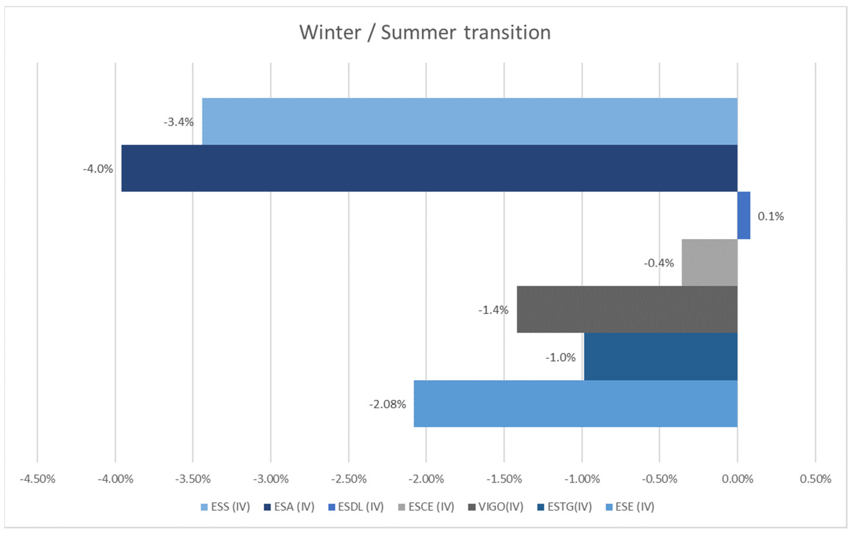
Figure 31 presents a horizontal bar chart illustrating the variation in energy consumption across Higher Education Institutions (HEIs) during the transition from winter time to summer time. The analysis considers data from the week before and the week after the time change, which occurred on 26 March 2023, ensuring comparability by evaluating the same weekdays in both periods. The results reveal an overall trend of reduced energy consumption, with a general average decrease of −1.7%, indicating a moderate impact of the time change. With the exception of ESDL, all analyzed institutions recorded a decline, suggesting that the transition to summer time positively influences energy efficiency. The most significant reduction was observed at ESA (−4.0%), followed by ESS (−3.4%) and ESE (−2.1%). The University of Vigo reported a variation of −1.4%, while ESTG and ESCE registered smaller reductions of −1.0% and −0.4%, respectively. On the other hand, ESDL stands out as the only institution with a slight increase in consumption (+0.1%), which may be associated with specific energy demand characteristics or operational patterns during the analyzed period. The prevailing trend of reduced consumption reinforces the correlation between the shift to summer time and the decrease in energy demand in HEIs.

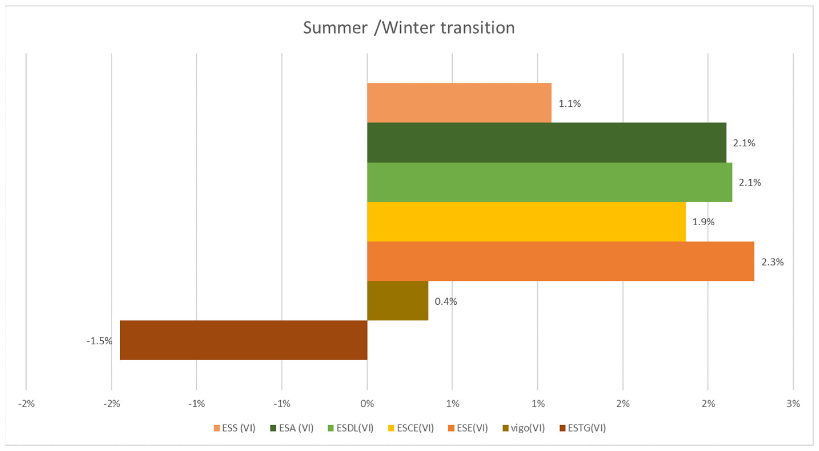
Figure 32 presents a horizontal bar chart analyzing the variation in energy consumption during the transition from summer time to winter time across various Higher Education Institutions (HEIs). The analysis is based on data from the week before and the week after the time change, which occurred on 29 October 2023, ensuring comparability by evaluating the same weekdays in both periods. The global average stands at +1.9%, indicating a moderate increase in energy consumption following the time change. With the exception of ESTG, all institutions recorded an increase, reflecting the impact of the transition to winter time on higher energy consumption. The highest increase was observed at ESE (+2.3%), followed by ESA and ESDL, both at +2.1%. The University of Vigo registered a more modest rise of +0.4%, while ESS showed a variation of +1.1%, close to the average. ESTG stands out as the only institution with a negative variation (−1.5%), a trend that may be explained by a high number of events held in the week prior to the time change, leading to atypically high energy consumption before the transition. The predominantly positive trend in the observed variations reinforces the correlation between the shift to winter time and increased energy consumption, suggesting that the reduction in natural daylight at the end of the day results in greater reliance on artificial lighting and potentially higher use of heating systems.

5. Conclusions

This study evaluates the impact of Daylight Saving Time (DST) transitions on energy consumption in Higher Education Institutions (HEIs), taking into account the importance of building characteristics, occupancy schedule, and operating conditions that influence energy consumption variability. The literature review highlights that the implementation of DST can contribute to energy savings in certain types of buildings; however, the overall effectiveness is highly dependent on local conditions, such as building occupancy, climate, and usage patterns.

The results showed that the transition to DST (winter to summer) led to an average reduction in energy consumption of 1.7%, while the return to standard time (summer to winter) led to an average increase of 1.2%. However, these effects varied considerably between institutions, highlighting the role of specific campus infrastructure, user density, and academic activity schedules. The highest consumption levels were associated with peak academic periods and extreme weather conditions, particularly due to heating and cooling loads. Conversely, lower consumption was recorded in months such as August and April, coinciding with holidays and reduced occupancy.

Weekly analysis before and after the time changes supported these trends, confirming the 1.7% average reduction in consumption during the DST transition. This was further validated by a t-test comparing the pre- and post-transition periods for each campus. Statistically significant changes (p < 0.05) were observed in several institutions—namely, ESEVC, ESCEV, ESDLM, ESAPL, and ESSVC—while others, such as ESTGVC and UVEM, did not show significant seasonal effects.

In addition, descriptive statistics and confidence intervals revealed that institutions with confidence intervals excluding zero showed significant seasonal variation, indicating a noticeable effect of DST transitions. This comparative analysis confirms that, although small, shifts in energy performance do occur in response to DST, with notable variability, depending on the institutional context.

While these results reinforce that DST may lead to modest reductions in electricity consumption, they also indicate that its overall effectiveness in HEIs is limited and highly context-specific.

From a policy standpoint, the findings suggest that DST alone may not be a reliable energy-saving measure in higher education environments, especially where occupancy patterns and HVAC systems are already optimized. Policymakers debating the future of DST should therefore consider its limited contribution to energy efficiency in such settings and instead focus on broader, more impactful strategies for demand reduction.

For institutional energy managers, the results highlight the importance of adapting HVAC and lighting control systems around DST transitions. Automated or smart control systems that respond dynamically to occupancy and daylight variation—rather than fixed schedules—could help maximize efficiency during time shifts. These adjustments may be especially relevant in months with variable usage and thermal loads.

Future studies should extend this analysis to a broader set of institutions in different climatic zones of the Iberian Peninsula. It would also be beneficial to explore the interplay between DST and other determinants of energy use, including the adoption of energy efficiency measures, occupant behavior, and the integration of smart energy management technologies.

References

1. European Commission. Proposal for a Directive of the European Parliament and of the Council Discontinuing Seasonal Changes of Time and Repealing Directive 2000/84/EC; European Commission: Brussels, Belgium, 2018.
2. Parliament, E. Summer-time arrangements: Directive 2000/84/EC evaluation. Eur. Parliam. Res. Serv. 2018, PE 611.006. [Google Scholar]
3. Kudela, P.; Havranek, T.; Herman, D.; Irsova, Z. Does daylight saving time save electricity? Evidence from Slovakia. Energy Policy 2020, 137, 111146. [Google Scholar] [CrossRef]
4. Flores, D.; Luna, E.M. An econometric evaluation of daylight saving time in Mexico. Energy 2019, 187, 116124. [Google Scholar] [CrossRef]
5. Petterini, F.; Signor, D.; Santos, P. The daylight saving borderline: Quasi-experimental analysis of the electric power consumption in Bahia and Tocantins. Nova Econ. 2018, 28, 943–964. [Google Scholar] [CrossRef]
6. Choi, S.; Pellen, A.; Masson, V. How does daylight saving time affect electricity demand? An answer using aggregate data from a natural experiment in Western Australia. Energy Econ. 2017, 66, 247–260. [Google Scholar] [CrossRef]
7. Ahuja, D.R.; SenGupta, D. Year-round daylight saving time will save more energy in India than corresponding DST or time zones. Energy Policy 2012, 42, 657–669. [Google Scholar] [CrossRef]
8. Guven, C.; Yuan, H.; Zhang, Q.; Aksakalli, V. When does daylight saving time save electricity? Weather and air-conditioning. Energy Econ. 2021, 98, 105216. [Google Scholar] [CrossRef]
9. Mirza, F.M.; Bergland, O. The impact of daylight saving time on electricity consumption: Evidence from southern Norway and Sweden. Energy Policy 2011, 39, 3558–3571. [Google Scholar] [CrossRef]
10. Havranek, T.; Herman, D.; Irsova, Z. Does Daylight Saving Save Electricity? A Meta-Analysis. Energy J. 2018, 39, 63–86. [Google Scholar] [CrossRef]
11. Rock, B.A. Impact of daylight saving time on residential energy consumption and cost. Energy Build. 1997, 25, 63–68. [Google Scholar] [CrossRef]
12. López, M. Daylight effect on the electricity demand in Spain and assessment of Daylight Saving Time policies. Energy Policy 2020, 140, 111419. [Google Scholar] [CrossRef]
13. Chen, X.; Wang, J.; Liang, R.; Mathas, E.; Lun, I.Y.F. Evaluation of the effect of daylight saving time on household lighting saving potential in six highly urbanised Chinese cities. Adv. Build. Energy Res. 2024, 18, 295–321. [Google Scholar] [CrossRef]
14. Krarti, M.; Hajiah, A. Analysis of impact of daylight time savings on energy use of buildings in Kuwait. Energy Policy 2011, 39, 2319–2329. [Google Scholar] [CrossRef]
15. Eggimann, S.; Mutschler, R.; Orehounig, K.; Fiorentini, M. Climate change shifts the trade-of between lower cooling and higher heating demand from daylight saving time in office buildings. Environ. Res. Lett. 2023, 18, 24001. [Google Scholar] [CrossRef]
16. Momani, M.A.; Yatim, B.; Ali, M.A.M. The impact of the daylight saving time on electricity consumption-A case study from Jordan. Energy Policy 2009, 37, 2042–2051. [Google Scholar] [CrossRef]
17. Kellogg, R.; Wolff, H. Daylight time and energy: Evidence from an Australian experiment. J. Environ. Econ. Manag. 2008, 56, 207–220. [Google Scholar] [CrossRef]
18. Karasu, S. The effect of daylight saving time options on electricity consumption of Turkey. Energy 2010, 35, 3773–3782. [Google Scholar] [CrossRef]
19. Bircan, Ç.; Wirsching, E. Daylight saving all year round? Evidence from a national experiment. Energy Econ. 2023, 127, 107093. [Google Scholar] [CrossRef]
20. Bellia, L.; Acosta, I.; Campano, M.Á.; Fragliasso, F. Impact of daylight saving time on lighting energy consumption and on the biological clock for occupants in office buildings. Sol. Energy 2020, 211, 1347–1364. [Google Scholar] [CrossRef]
21. Es-Sakali, N.; Pfafferott, J.; Mghazli, M.O.; Cherkaoui, M. Towards climate-responsive net zero energy rural schools: A multi-objective passive design optimization with bio-based insulations, shading, and roof vegetation. Sustain. Cities Soc. 2025, 120, 106142. [Google Scholar] [CrossRef]
Figure 1. Annual scientific production on DST and energy consumption.
Energies 18 03157 g001
Figure 2. Localization of the seven studied buildings.
Energies 18 03157 g002
Figure 3. Energy map of ESCEV CAMPUS.
Energies 18 03157 g003
Figure 4. Energy map of ESDLM CAMPUS.
Energies 18 03157 g004
Figure 5. Energy map of ESAPL CAMPUS.
Energies 18 03157 g005
Figure 6. Energy map of ESEVC CAMPUS.
Energies 18 03157 g006
Figure 7. Energy map of ESSVC CAMPUS.
Energies 18 03157 g007
Figure 8. Energy map of ESTGVC CAMPUS.
Energies 18 03157 g008
Figure 9. Energy map of UVEM CAMPUS.
Energies 18 03157 g009
Figure 10. Total monthly consumption and average hourly consumption per month for ESCEV.
Energies 18 03157 g010
Figure 11. Average hourly consumption (a) and daily consumption (b) in March and April 2023 (ESCEV).
Energies 18 03157 g011
Figure 12. Average hourly consumption (a) and daily consumption (b) in October and November 2023 (ESCEV).
Energies 18 03157 g012
Figure 13. Total monthly consumption and average hourly consumption per month for ESDLM.
Energies 18 03157 g013
Figure 14. Average hourly consumption (a) and daily consumption (b) in March and April 2023 (ESDLM).
Energies 18 03157 g014
Figure 15. Average hourly consumption (a) and daily consumption (b) in October and November 2023 (ESDLM).
Energies 18 03157 g015
Figure 16. Total monthly consumption and average hourly consumption per month for ESAPL.
Energies 18 03157 g016
Figure 17. Average hourly consumption (a) and daily consumption (b) in March and April 2023 (ESAPL).
Energies 18 03157 g017
Figure 18. Average hourly consumption (a) and daily consumption (b) in October and November 2023 (ESAPL).
Energies 18 03157 g018
Figure 19. Total monthly consumption and average hourly consumption per month for ESEVC.
Energies 18 03157 g019
Figure 20. Average hourly consumption (a) and daily consumption (b) in March and April 2023 (ESEVC).
Energies 18 03157 g020
Figure 21. Average hourly consumption (a) and daily consumption (b) in October and November 2023 (ESEVC).
Energies 18 03157 g021
Figure 22. Total monthly consumption and average hourly consumption per month for ESSVC.
Energies 18 03157 g022
Figure 23. Average hourly consumption (a) and daily consumption (b) in March and April 2023 (ESSVC).
Energies 18 03157 g023
Figure 24. Average hourly consumption (a) and daily consumption (b) in October and November 2023 (ESSVC).
Energies 18 03157 g024
Figure 25. Total monthly consumption and average hourly consumption per month for ESTGVC.
Energies 18 03157 g025
Figure 26. Average hourly consumption (a) and daily consumption (b) in March and April 2023 (ESTGVC).
Energies 18 03157 g026
Figure 27. Average hourly consumption (a) and daily consumption (b) in October and November 2023 (ESTGVC).
Energies 18 03157 g027
Figure 28. Total monthly consumption and average hourly consumption per month for UVEM.
Energies 18 03157 g028
Figure 29. Average hourly consumption (a) and daily consumption (b) in March and April 2023 (UVEM).
Energies 18 03157 g029
Figure 30. Average hourly consumption (a) and daily consumption (b) in October and November 2023 (UVEM).
Energies 18 03157 g030
Figure 31. Comparison of energy consumption before and after the time change from winter to summer in HEIs.
Energies 18 03157 g031
Figure 32. Comparison of energy consumption before and after the time change to summer time in HEIs.
Energies 18 03157 g032