Multi-Energy-Microgrid Energy Management Strategy Optimisation Using Deep Learning

Abstract

Renewable power generation is unpredictable due to its intermittency, making grid-connected microgrids difficult to operate, control, and manage. Currently used prediction models for electricity, heat, gas, and hydrogen multi-energy complementary microgrids with the carbon trading mechanism are inefficient as they cannot account for all eventualities and are not well studied. Therefore, a two-stage robust optimisation model based on Bidirectional Temporal Convolutional Networks (BiTCN) and Transformer prediction for electricity, heat, gas, and hydrogen multi-energy complementary microgrids with a carbon trading mechanism is proposed to solve this problem. First, BiTCN extracts implicit wind speed and wind power output sequences from historical data and feeds it into the Transformer model for point prediction using the attention mechanism. Ablation computation modelling is then performed. The proposed prediction model’s Mean Absolute Error (MAE) is found to be 1.3512, and its R² is 0.9683, proving its efficacy and reliability. Second, the proposed model is used to perform interval prediction in two typical scenarios: high wind power and low wind power. After constructing the robust optimisation model uncertainty set based on the prediction results, simulation experiments are performed on the proposed optimisation model. The simulation results suggest that the proposed optimisation model enhances renewable energy use, emissions reductions, microgrid operating costs, and system reliability. The study also reveals that the total system cost and carbon emission cost in the low wind scenario are 283% (2.83 times) and 314% (3.14 times) higher than in the high wind scenario; hence, a significant percentage of renewable energy is needed for microgrid stability.

1. Introduction

Energy and environmental issues are two important challenges to sustainable global development. In most countries around the world, power generation still relies on fossil energy sources such as coal-fired power stations, which creates serious energy waste and environmental problems. As the population grows rapidly, so does residential electricity consumption, impacting the stability of urban power grids [1]. In recent years, smart grids and microgrids have been progressively built to address the challenges of overloading the grid. Smart grids, as opposed to microgrids, are vast, networked systems that employ digital technologies to track, regulate, and oversee the electricity flow throughout the entire grid. In contrast, microgrids are smaller, more compact, localised systems that often function either alone or in tandem with a larger smart grid. Microgrids, integral to the smart grid, consist of clusters of distributed generators (DGs), energy storage systems (ESS), loads, and various monitoring and protection devices [2]. By interacting with the main grid and facilitating the distributed renewable energy resources (wind and photovoltaic), microgrids can enhance efficient energy management and grid stability and reduce the grid’s environmental impact [3]. However, the intermittency and uncertainty of renewable energy output in microgrids make its application challenging, and their energy management strategies have attracted considerable attention [4]. To ensure the balance of power supplied by the microgrid, the uncertainty of renewable energy output on the supply side is a factor that must be considered in the energy management of the microgrid [5]. The accurate description of the uncertainty in renewable energy output relies on the progress of load forecasting methods. Traditional forecasting approaches such as MLP and decision trees have been insufficient in accurately characterising the uncertainty of renewable energy output, thereby negatively impacting the results of microgrid energy management.

To address this challenge, in recent years, with the progress of prediction theory and artificial intelligence technology as well as the energy internet environment, power consumption data, weather data, wind power generation data, photovoltaic power generation data, system operation, and system maintenance data can be collected, which can provide an important foundation for the training of prediction models [6]. Deep learning models can extract the mapping relationship between numerical weather prediction (NWP) data such as wind speed and wind power data. This relationship can be used to predict future wind power generation output with significant nonlinear fitting capabilities [7]. Deep learning models that are commonly used to predict wind power generation sequences are Long-term Short-term Memory Networks (LSTM), Temporal Convolutional Networks (TCN), Transformer, Generative Adversarial Network (GAN), etc. [8]. TCN maintains long-term sequence prediction performance by utilising residual blocks and dilated causal convolution for better time series prediction: Shao et al. [9] achieved higher accuracy than LSTM by adjusting the receptive field of TCN to predict the wind energy components at different frequencies. However, TCN models only extract forward time information; they ignore backward information. The Bidirectional Temporal Convolutional Network (BiTCN) model proposed by Graves et al. [10] can capture bidirectional information of the time series. Experimental results show that its prediction accuracy is higher than that of unidirectional TCN. However, due to the considerable volatility of wind power, the prediction results using only deep learning models are not satisfactory [11]. Many existing predictive models rely on single inputs or simpler model structures that ignore the complex time-series correlations between multiple variables. Most methods deal with linear relationships between only some of the input variables and fail to adequately account for nonlinear interactions and long-term dependencies between variables. The prediction results are often inadequate. To address this challenge, the development of hybrid models is an effective solution to achieve higher accuracy in wind energy forecasting. Meanwhile, the introduction of attention mechanisms in deep learning hybrid prediction models can effectively capture the key information in the complex spatio-temporal features of wind power or photovoltaic power and improve the model’s ability to focus on important time steps and feature dimensions, thus improving the accuracy and robustness of the model’s predictions. Liu et al. [12] suggested a new model that mixes convolutional neural networks (CNNs) with Bidirectional Long Short-Term Memory (BiLSTM) networks, calling it the CNN-BiLSTM model for predicting PV power. They reported that the hybrid model had a lower Mean Absolute Error (MAE) and greater stability than the basic model when dealing with weather-related uncertainties in grid operations. Cheng et al. [13] proposed a domain-knowledge integrated Transformer (DKFormer) model to correct wind power forecasting errors using specialised data processing modules and boundary constraints using measured power and NWP data. With the increasing demand for simplified microgrid energy management models, reinforcement learning methods have become a hot topic in recent years, and they have been applied to address issues in microgrid energy management. As a model-free intelligent algorithm, reinforcement learning can learn and find optimal solutions to optimisation problems in uncertain and dynamic environments. Chen et al. [14] proposed a model-free deep reinforcement learning (DRL)-based energy management strategy (EMS) for regenerative braking energy storage systems (RBESS) in railway power systems, formulating the problem as a Markov decision process (MDP) with a multistage reward function. Their EMS demonstrated performance superior to that of traditional methods by over 5% in energy management objectives. Zhao et al. [15] suggested an enhanced duelling double deep Q network algorithm with mixed penalty function (EN-D3QN-MPF) for microgrid energy management, integrating renewable sources and flexible loads while optimising low-carbon economic operation and EV charging satisfaction, demonstrating performance superior to GA, PSO, and other DRL methods through real-world case validation.

Current research on neural network-based prediction methods predominantly focuses on the dispatch of a single energy source. This approach limits the ability to coordinate and optimise multiple energy sources in a microgrid, thereby reducing the overall efficiency of the system [16]. In addition, with the advancement of the dual-carbon goal, a multi-energy complementary microgrid operation model considering carbon quota and carbon trading is necessary in microgrid energy management. To predict wind power or photovoltaic power generation, deep learning-based optimisation methods can account for uncertainty, distribution, and complex nonlinear relationships through data-driven optimisation [17], compared with traditional optimisation, which relies on conservative assumptions in relation to the efficient dispatch of power and load changes in the microgrid. Li et al. [18] reported a data-driven two-stage distributionally optimised model for community integrated energy systems, combining a Wasserstein-GAN scenario generation method with integrated demand response to achieve lower operating costs, higher renewable energy utilisation, and faster computation compared to conventional methods while balancing economic operation and system robustness. Another data-driven distributional optimisation (DRO) method for integrated energy system scheduling, using CGAN-generated scenarios and a hybrid 1-norm/∞-norm uncertainty was presented by Ma et al. [19] to reduce operating costs and enhance computational efficiency. Yang et al. [20] suggested a two-stage microgrid scheduling framework that combines improved Gaussian process regression forecasting with adaptive optimisation, reducing the impacts of renewable energy uncertainty through day-ahead worst-case scenario planning and intra-day rolling optimisation for cost reduction while maintaining system reliability. Zhu et al. [21] came up with a two-stage optimisation model for residential energy hubs that simultaneously optimises energy market bidding and flexible ramp product provision, using an LSTM-based interval prediction method to reduce solution conservatism while improving economic performance through multi-market participation. Xu et al. [22] outlined a photovoltaic mechanism/data-fusion-driven adaptive optimisation strategy for combined heat and power microgrids, combining clear-sky radiation modelling with data-driven error confidence intervals to minimise operating costs while effectively mitigating PV output uncertainty. The simulated results were compared with the analytical solutions. Although numerous optimisation models have been reported in the open literature, including those mentioned above, there are significant knowledge gaps, and uncertainties remain.

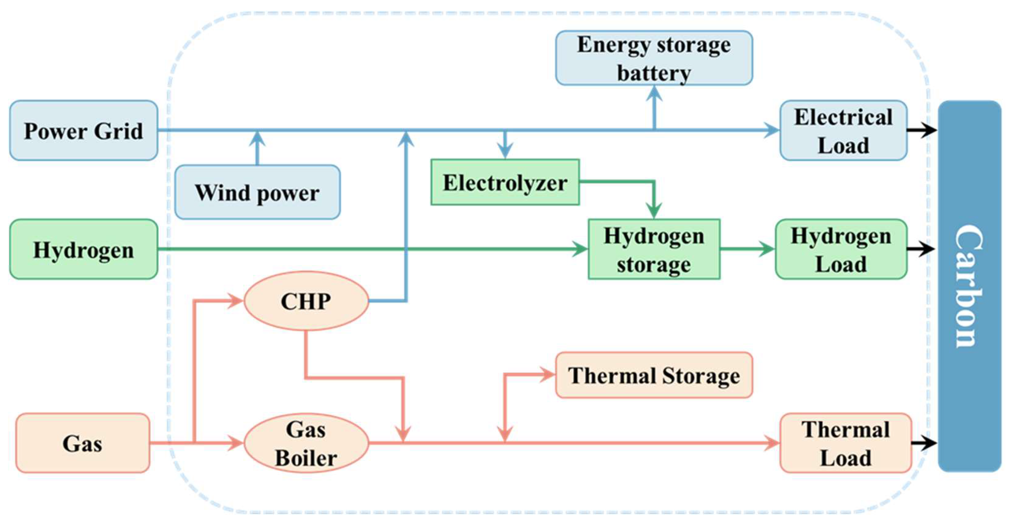
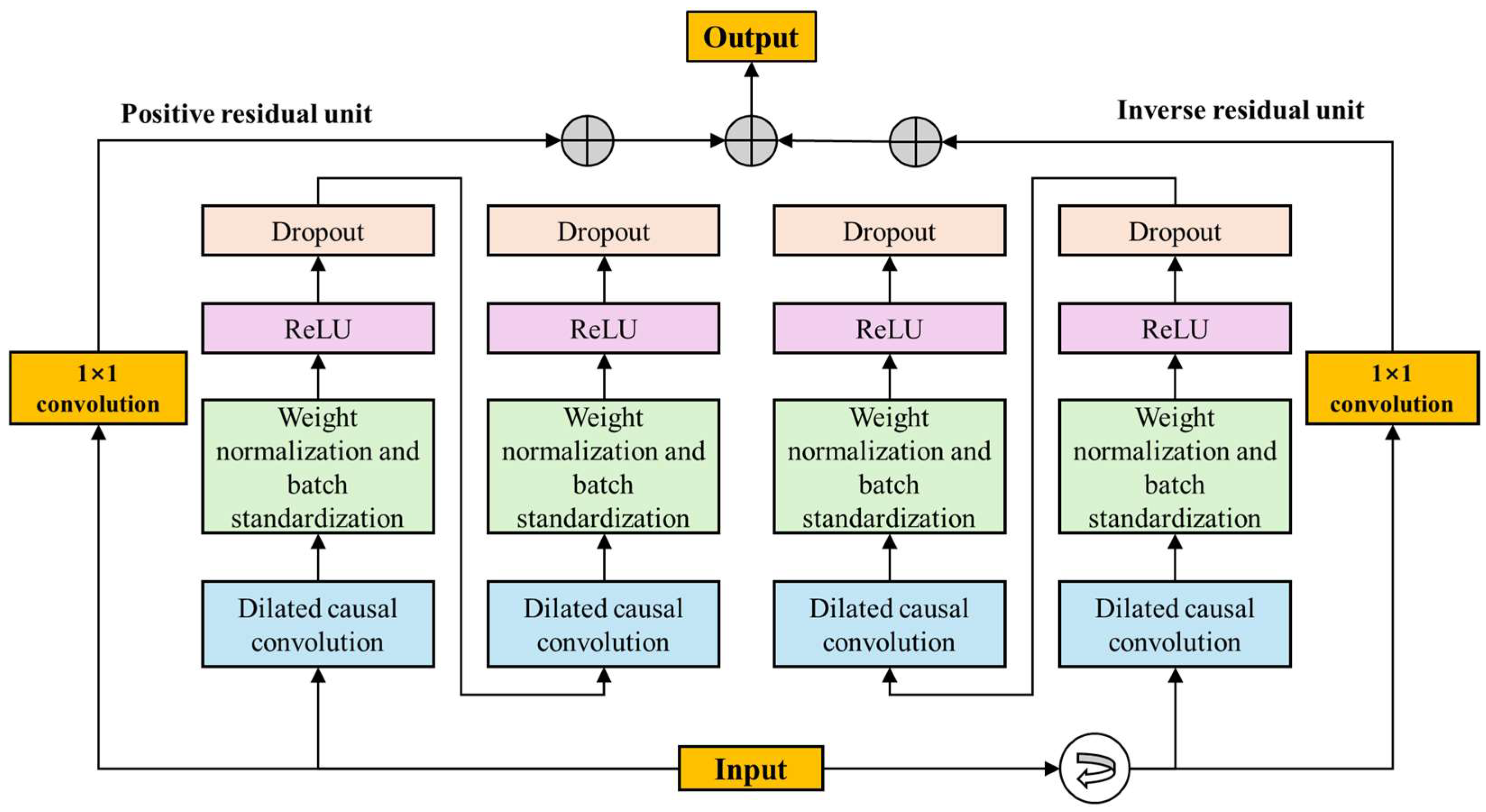
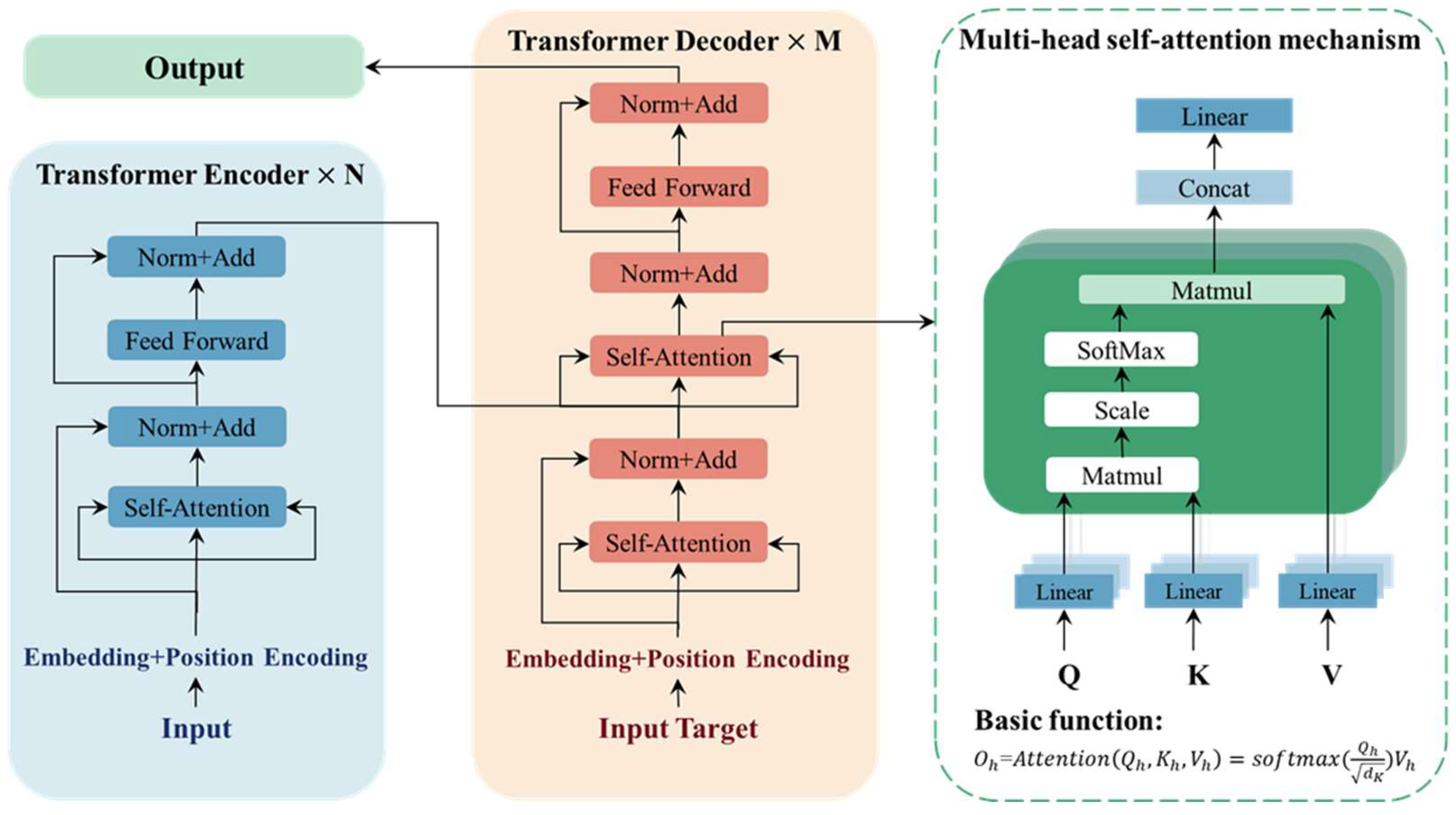
Given the urgent need for a dependable and effective way to manage microgrid energy, this study aims to create a strong optimisation model for electricity/heat/gas/hydrogen multi-energy complementary microgrids. The model includes a carbon trading system. This model will handle the uncertainty of wind power output, which will be predicted and managed using a deep learning model called BiTCN-Transformer. The model is based on multimodal time series; the BiTCN captures the local temporal dependencies, while the Transformer model dynamically learns the correlations between different time points. By combining the two, the model can pay attention to both nearby and distant information, helping it to better understand the various patterns in the time data, which makes processing the data more thorough and precise and ultimately improves the model’s ability to make predictions. Subsequently, microgrid energy management experiments are to be conducted under two typical scenarios: a high wind power scenario and a low wind power scenario, combined with tariff and load data, to verify the effectiveness of the proposed model in coping with the supply-side uncertainty of microgrids and the synergy of multi-energy complements at the same time. The purpose is to reduce the operating cost of microgrids, improve the utilisation rate of renewable energy, reduce emissions, and ultimately enhance the reliability of the system’s operation. The following are the study’s primary contributions:

(a)

A multi-energy complementary microgrid energy management framework for electricity, heat, gas, and hydrogen with a carbon trading mechanism is proposed, which contains multi-energy complementary multiple resource loads and a carbon trading model.

(b)

A deep learning model using BiTCN-Transformer is suggested to forecast wind power output and make specific predictions and tests are done to confirm that this model performs better than others based on different evaluation criteria.

(c)

Based on the point prediction results, interval prediction is performed in two typical cases, a high wind power scenario and a low wind power scenario, using a nonparametric kernel density estimation model and a confidence interval calculation method to construct a boxed uncertainty set for the robust operational optimisation model.

2. Approach and Methodology

In this study, the intent is to develop a robust two-stage optimisation model for multi-energy complementary microgrids based on deep learning to deal with wind power output uncertainty and carbon trading mechanisms. The general model is divided into an optimisation model and a prediction model. In the optimisation model, each component of the proposed multi-energy complementary microgrid energy management system is modelled, followed by a detailed description of the talking trading mechanism and the two-stage robust optimisation model. In the prediction model, the mechanism of the proposed BiTCN-Transformer deep learning combination model is introduced. The model part lays the foundation for the subsequent deep learning point prediction and interval prediction to construct the uncertainty set as well as the low-carbon optimisation plan for microgrids.

2.1. Optimisation Model

A two-stage robust optimisation model is proposed here, integrating carbon trading mechanisms for electricity/gas/heat/hydrogen complementary microgrids. As shown in Figure 1, the system architecture contains wind turbines combined with multiple energy conversion and storage components: combined heat and power (CHP) units, gas boilers, electrolytic cells (EC), hydrogen storage (HS) units, electrical energy storage (EES) units, and thermal energy storage (TES) units. Three types of load demands are considered: electrical, hydrogen, and thermal loads. The electrical load is jointly supplied through power exchange with the main grid, wind turbines, and CHP units, with surplus electricity being sold to the main grid. The hydrogen demands of fuel cell vehicles is fulfilled through on-site electrolysis and external procurement. The thermal load is satisfied by CHP units and gas boilers. Energy storage units (EES and TES) are employed to coordinate supply–demand balance. A CO₂ trading mechanism incorporating allowance allocation and trading volume is integrated into the system. The optimisation objective aims to minimise total energy costs while addressing wind power uncertainties and operational constraints. This is achieved by rationally scheduling (a) dispatchable DGs’ outputs, (b) power exchange with the main grid, (c) charge/discharge cycles of EES and TES units, and (d) HS operations. The total cost structure comprises four components: electricity trading costs with the main grid, natural gas procurement costs, hydrogen purchase costs, and maintenance expenses for DGs.

2.1.1. Objective Function

The goal of microgrid scheduling is to reduce the overall cost, which encompasses the transaction cost between the microgrid and the main grid, the cost of purchasing natural gas, the cost of acquiring hydrogen, and the maintenance expenses associated with the distributed generators within the microgrid. The objective function is presented in Equation (1).

$$\min \sum _{\mathrm{k}}\left[\left({\mathrm{\rho }}_{\mathrm{k}}^{\mathrm{p}\mathrm{u}\mathrm{r}\mathrm{c}\mathrm{h}\mathrm{a}\mathrm{s}\mathrm{e}}·{\mathrm{P}}_{\mathrm{k}}^{\mathrm{g}\mathrm{r}\mathrm{i}\mathrm{d},\mathrm{i}\mathrm{m}\mathrm{p}}-{\mathrm{\rho }}_{\mathrm{k}}^{\mathrm{s}\mathrm{a}\mathrm{l}\mathrm{e}}·{\mathrm{P}}_{\mathrm{k}}^{\mathrm{g}\mathrm{r}\mathrm{i}\mathrm{d},\mathrm{e}\mathrm{x}\mathrm{p}}\right)\cdot \Delta \mathrm{T}+{\mathrm{F}}_{\mathrm{k}}^{\mathrm{G}\mathrm{a}\mathrm{s}}·{\mathrm{\gamma }}_{\mathrm{k}}^{\mathrm{F}\mathrm{u}\mathrm{e}\mathrm{l}}+{\mathrm{S}}_{\mathrm{k}}^{\mathrm{H}}·{\mathrm{\gamma }}_{\mathrm{k}}^{\mathrm{H}}\right]+{\mathrm{C}}_{\mathrm{G}\mathrm{e}\mathrm{n}}+{\mathrm{C}}_{\mathrm{E}}$$

(1)

where ${\mathrm{\rho }}_{\mathrm{k}}^{\mathrm{p}\mathrm{u}\mathrm{r}\mathrm{c}\mathrm{h}\mathrm{a}\mathrm{s}\mathrm{e}}$ and ${\mathrm{\rho }}_{\mathrm{k}}^{\mathrm{s}\mathrm{a}\mathrm{l}\mathrm{e}}$ are the power purchase price of the microgrid from the main grid and the power sale price of the microgrid to the main grid at the time k, respectively; ${\mathrm{P}}_{\mathrm{k}}^{\mathrm{g}\mathrm{r}\mathrm{i}\mathrm{d},\mathrm{i}\mathrm{m}\mathrm{p}}$ and ${\mathrm{P}}_{\mathrm{k}}^{\mathrm{g}\mathrm{r}\mathrm{i}\mathrm{d},\mathrm{e}\mathrm{x}\mathrm{p}}$ are the power purchase of the microgrid from the main grid and the power sale of the microgrid to the main grid at the time k, respectively; ${\mathrm{F}}_{\mathrm{k}}^{\mathrm{G}\mathrm{a}\mathrm{s}}$ and ${\mathrm{\gamma }}_{\mathrm{k}}^{\mathrm{F}\mathrm{u}\mathrm{e}\mathrm{l}}$ are the natural gas purchase volume and purchase price of the microgrid at the time k, respectively; ${\mathrm{S}}_{\mathrm{k}}^{\mathrm{H}}$ and ${\mathrm{\gamma }}_{\mathrm{k}}^{\mathrm{H}}$ are the hydrogen procurement volume and the buying price of the microgrid. ${\mathrm{C}}_{\mathrm{G}\mathrm{e}\mathrm{n}}$ is the maintenance cost of DGs in the microgrid.

The total maintenance cost is shown in Equation (2).

$${\mathrm{C}}_{\mathrm{M}\mathrm{a}\mathrm{i}\mathrm{n}\mathrm{t}\mathrm{a}\mathrm{i}\mathrm{n}}={\mathrm{C}}_{\mathrm{O}\mathrm{M}}^{\mathrm{W}\mathrm{T}}+{\mathrm{C}}_{\mathrm{O}\mathrm{M}}^{\mathrm{C}\mathrm{H}\mathrm{P}}+{\mathrm{C}}_{\mathrm{O}\mathrm{M}}^{\mathrm{B}\mathrm{o}\mathrm{l}\mathrm{i}\mathrm{e}\mathrm{r}}+{\mathrm{C}}_{\mathrm{O}\mathrm{M}}^{\mathrm{T}\mathrm{E}\mathrm{S}}+{\mathrm{C}}_{\mathrm{O}\mathrm{M}}^{\mathrm{H}\mathrm{S}}+{\mathrm{C}}_{\mathrm{O}\mathrm{M}}^{\mathrm{E}\mathrm{C}}+{\mathrm{C}}_{\mathrm{O}\mathrm{M}}^{\mathrm{E}\mathrm{E}\mathrm{S}}$$

(2)

where ${\mathrm{C}}_{\mathrm{O}\mathrm{M}}^{\mathrm{W}\mathrm{T}}$, ${\mathrm{C}}_{\mathrm{O}\mathrm{M}}^{\mathrm{C}\mathrm{H}\mathrm{P}}$, and ${\mathrm{C}}_{\mathrm{O}\mathrm{M}}^{\mathrm{B}\mathrm{o}\mathrm{l}\mathrm{i}\mathrm{e}\mathrm{r}}$ are the maintenance costs for the wind power unit, cogeneration unit, and gas boiler. ${\mathrm{C}}_{\mathrm{O}\mathrm{M}}^{\mathrm{T}\mathrm{E}\mathrm{S}}$, ${\mathrm{C}}_{\mathrm{O}\mathrm{M}}^{\mathrm{H}\mathrm{S}}$, ${\mathrm{C}}_{\mathrm{O}\mathrm{M}}^{\mathrm{E}\mathrm{C}}$, and ${\mathrm{C}}_{\mathrm{O}\mathrm{M}}^{\mathrm{E}\mathrm{E}\mathrm{S}}$ are the maintenance costs for the TES unit, the HS tank, the EES unit, and the electrolyser, respectively.

Specific formulas for the maintenance costs of each DG are shown in Equations (3)–(9).

$${\mathrm{C}}_{\mathrm{O}\mathrm{M}}^{\mathrm{W}\mathrm{T}}=\sum _{\mathrm{k}}{\mathrm{W}}_{\mathrm{k}}^{\mathrm{W}\mathrm{T}}·{\mathsf{\xi }}_{\mathrm{W}\mathrm{T}}·\Delta \mathrm{K}$$

(3)

$${\mathrm{C}}_{\mathrm{O}\mathrm{M}}^{\mathrm{C}\mathrm{H}\mathrm{P}}=\sum _{\mathrm{k}}\left({\mathrm{W}}_{\mathrm{k}}^{\mathrm{E}\mathrm{C}\mathrm{H}\mathrm{P}}+{\mathrm{W}}_{\mathrm{k}}^{\mathrm{T}\mathrm{C}\mathrm{H}\mathrm{P}}\right)\cdot {\mathsf{\xi }}_{\mathrm{C}\mathrm{H}\mathrm{P}}\cdot \Delta \mathrm{K}$$

(4)

$${\mathrm{C}}_{\mathrm{O}\mathrm{M}}^{\mathrm{B}\mathrm{o}\mathrm{l}\mathrm{i}\mathrm{e}\mathrm{r}}=\sum _{\mathrm{k}}{\mathrm{W}}_{\mathrm{k}}^{\mathrm{T}\mathrm{h}\mathrm{r}\mathrm{m}}\cdot {\mathsf{\xi }}_{\mathrm{B}\mathrm{o}\mathrm{l}\mathrm{i}\mathrm{e}\mathrm{r}}\cdot \Delta \mathrm{K}$$

(5)

$${\mathrm{C}}_{\mathrm{O}\mathrm{M}}^{\mathrm{T}\mathrm{E}\mathrm{S}}=\sum _{\mathrm{k}}\left({\mathrm{W}}_{\mathrm{c}\mathrm{h},\mathrm{k}}^{\mathrm{T}\mathrm{E}\mathrm{S}}+{\mathrm{W}}_{\mathrm{d}\mathrm{c}\mathrm{h},\mathrm{k}}^{\mathrm{T}\mathrm{E}\mathrm{S}}\right)\cdot {\mathsf{\xi }}_{\mathrm{T}\mathrm{E}\mathrm{S}}\cdot \Delta \mathrm{K}$$

(6)

$${\mathrm{C}}_{\mathrm{O}\mathrm{M}}^{\mathrm{H}\mathrm{S}}=\sum _{\mathrm{k}}\left({\mathrm{V}}_{\mathrm{ch},\mathrm{k}}^{\mathrm{H}\mathrm{S}}+{\mathrm{V}}_{\mathrm{d}\mathrm{c}\mathrm{h},\mathrm{k}}^{\mathrm{H}\mathrm{S}}\right)\cdot {\mathsf{\xi }}_{\mathrm{H}\mathrm{S}}\cdot \Delta \mathrm{K}$$

(7)

$${\mathrm{C}}_{\mathrm{O}\mathrm{M}}^{\mathrm{E}\mathrm{E}\mathrm{S}}=\sum _{\mathrm{k}}\left({\mathrm{P}}_{\mathrm{c}\mathrm{h},\mathrm{k}}^{\mathrm{E}\mathrm{E}\mathrm{S}}+{\mathrm{P}}_{\mathrm{d}\mathrm{c}\mathrm{h},\mathrm{k}}^{\mathrm{E}\mathrm{E}\mathrm{S}}\right)\cdot {\mathsf{\xi }}_{\mathrm{E}\mathrm{E}\mathrm{S}}\cdot \Delta \mathrm{K}$$

(8)

$${\mathrm{C}}_{\mathrm{O}\mathrm{M}}^{\mathrm{E}\mathrm{C}}=\sum _{\mathrm{k}}{\mathrm{P}}_{\mathrm{k}}^{\mathrm{E}\mathrm{C}}\cdot {\mathsf{\xi }}_{{}_{\mathrm{E}\mathrm{C}}}\cdot \Delta \mathrm{K}$$

(9)

Equation (3) is the formula for the total maintenance cost of microgrids. ${\mathrm{W}}_{\mathrm{k}}^{\mathrm{W}\mathrm{T}}$ denotes the forecasted wind power output at a given time, with ${\mathsf{\xi }}_{\mathrm{W}\mathrm{T}}$ representing its maintenance coefficient. Equations (4)–(9) are specific formulas for the maintenance cost of each DG. ${\mathrm{W}}_{\mathrm{k}}^{\mathrm{E}\mathrm{C}\mathrm{H}\mathrm{P}}$ and ${\mathrm{W}}_{\mathrm{k}}^{\mathrm{T}\mathrm{C}\mathrm{H}\mathrm{P}}$ denote the electrical and thermal outputs, with ${\mathsf{\xi }}_{\mathrm{C}\mathrm{H}\mathrm{P}}$ representing the maintenance coefficient. Thermal output ${\mathrm{W}}_{\mathrm{k}}^{\mathrm{T}\mathrm{h}\mathrm{r}\mathrm{m}}$ incorporates the maintenance coefficient ${\mathsf{\xi }}_{\mathrm{B}\mathrm{o}\mathrm{l}\mathrm{i}\mathrm{e}\mathrm{r}}$. The charging/discharging power (${\mathrm{W}}_{\mathrm{c}\mathrm{h},\mathrm{k}}^{\mathrm{T}\mathrm{E}\mathrm{S}}$, ${\mathrm{W}}_{\mathrm{d}\mathrm{c}\mathrm{h},\mathrm{k}}^{\mathrm{T}\mathrm{E}\mathrm{S}}$) incorporates the maintenance coefficient ${\mathsf{\xi }}_{\mathrm{T}\mathrm{E}\mathrm{S}}$. Hydrogen storage/discharge rates (${\mathrm{V}}_{\mathrm{ch},\mathrm{k}}^{\mathrm{H}\mathrm{S}}$, ${\mathrm{V}}_{\mathrm{d}\mathrm{c}\mathrm{h},\mathrm{k}}^{\mathrm{H}\mathrm{S}}$) incorporate the maintenance coefficient ${\mathsf{\xi }}_{\mathrm{H}\mathrm{S}}$. Electrical storage operations (${\mathrm{P}}_{\mathrm{c}\mathrm{h},\mathrm{k}}^{\mathrm{E}\mathrm{E}\mathrm{S}}$, ${\mathrm{P}}_{\mathrm{d}\mathrm{c}\mathrm{h},\mathrm{k}}^{\mathrm{E}\mathrm{E}\mathrm{S}}$) incorporate the maintenance coefficient ${\mathsf{\xi }}_{\mathrm{E}\mathrm{E}\mathrm{S}}$. Power consumption ${\mathrm{P}}_{\mathrm{t}}^{\mathrm{E}\mathrm{C}}$ used for hydrogen production associates with ${\mathsf{\xi }}_{{}_{\mathrm{E}\mathrm{C}}}$.

The carbon trading mechanism incentivises emissions reduction through market-based quota transactions in which emission rights function as tradable commodities. This market-driven approach promotes renewable integration and operational optimisation in multi-energy microgrids. The main carbon trading mechanism models are shown in Equation (10).

$${\mathrm{E}}_0=\sum _{\mathrm{i}\in \mathrm{F}}{\mathrm{T}}_{\mathrm{i}}\cdot {\mathrm{P}}_{\mathrm{i},\mathrm{h}}^{\mathrm{m}\mathrm{a}\mathrm{x}}$$

(10)

where $\mathrm{F}$ stands for high carbon emitting equipment, ${\mathrm{T}}_{\mathrm{i}}$ is the carbon emission factor per unit of electricity of the equipment (baseline value 0.57 t/MWh [23]), and ${\mathrm{P}}_{\mathrm{i},\mathrm{h}}^{\mathrm{m}\mathrm{a}\mathrm{x}}$ is the maximum thermal power output of the equipment i at time h.

The actual carbon emissions calculation mainly quantifies the real carbon emissions of the system operation, as shown in Equation (11).

$${\mathrm{E}}_{\mathrm{a}}=\sum _{\mathrm{j}\in \mathrm{C}}{\mathrm{K}}_{\mathrm{j}}\cdot {\mathrm{P}}_{\mathrm{j},\mathrm{k}}+{\mathrm{K}}_{\mathrm{g}\mathrm{r}\mathrm{i}\mathrm{d}}\cdot {\mathrm{E}}_{\mathrm{g}\mathrm{r}\mathrm{i}\mathrm{d},\mathrm{k}}+{\mathrm{K}}_{\mathrm{g}\mathrm{a}\mathrm{s}}\cdot {\mathrm{V}}_{\mathrm{g}\mathrm{a}\mathrm{s},\mathrm{k}}$$

(11)

where $\mathrm{C}$ is the carbon source pool; ${\mathrm{K}}_{\mathrm{j}}$ is the carbon intensity of equipment j, of which the baseline value is 0.52 kg CO₂/kWh [24]; ${\mathrm{P}}_{\mathrm{j},\mathrm{k}}$ is the output power of equipment j at time period k; ${\mathrm{K}}_{\mathrm{g}\mathrm{r}\mathrm{i}\mathrm{d}}$ is the marginal carbon emission factor of grid purchased power; ${\mathrm{E}}_{\mathrm{g}\mathrm{r}\mathrm{i}\mathrm{d},\mathrm{k}}$ is the amount of grid purchased power at time period k; ${\mathrm{K}}_{\mathrm{g}\mathrm{a}\mathrm{s}}$ is the natural gas combustion carbon emission factor; and ${\mathrm{V}}_{\mathrm{g}\mathrm{a}\mathrm{s},\mathrm{k}}$ is the natural gas consumption for time period k.

Adding the reward and punishment mechanism to the above carbon quota and carbon emission modelling is shown in Equation (12).

$${\mathrm{C}}_{\mathrm{C}{\mathrm{O}}_2}=\left\{\begin{array}{c}-{\mathrm{P}}_{\mathrm{C}{\mathrm{O}}_2}\cdot ({\mathrm{E}}_0-{\mathrm{E}}_{\mathrm{a}})\cdot {\mathrm{\eta }}_{\mathrm{r}\mathrm{e}\mathrm{w}\mathrm{a}\mathrm{r}\mathrm{d}},{\mathrm{E}}_{\mathrm{a}}\le {\mathrm{E}}_0\\ {\mathrm{P}}_{\mathrm{C}{\mathrm{O}}_2}\cdot ({\mathrm{E}}_{\mathrm{a}}-{\mathrm{E}}_0)\cdot {\mathrm{\eta }}_{\mathrm{p}\mathrm{e}\mathrm{n}\mathrm{a}\mathrm{l}\mathrm{t}\mathrm{y}},{\mathrm{E}}_{\mathrm{a}}>{\mathrm{E}}_0\end{array}\right.$$

(12)

where ${\mathrm{P}}_{\mathrm{C}{\mathrm{O}}_2}$ is the market price of carbon trading costs, the baseline value of which is 68.54 (yuan/t) [24].

2.1.2. Constraints

The constraints proposed in this study include hydrogen-related constraints, TES unit constraints, electric energy storage unit constraints, microgrid electric/thermal/hydrogen supply–demand balance constraints, distributed power production constraints, natural gas input limitations, and power transfer constraints. Here is a description of the specific constraints:

Hydrogen-related constraints

Electrolysis tanks can be used to meet hydrogen loads by producing hydrogen through electrolysis when electricity prices are low [25]. The constraints associated with hydrogen production and storage are shown in Equations (13)–(15).

$${\mathrm{Q}}_{\mathrm{k}}^{\mathrm{E}\mathrm{C}}={\mathrm{P}}_{\mathrm{k}}^{\mathrm{E}\mathrm{C}}\cdot {\mathrm{\eta }}_{\mathrm{E}\mathrm{C}}\cdot {\mathrm{\rho }}_{\mathrm{E}\mathrm{C}}\cdot \Delta \mathrm{K}$$

(13)

$${\mathrm{Q}}_{\mathrm{k}}^{\mathrm{H}\mathrm{S}}={\mathrm{Q}}_{\mathrm{k}-1}^{\mathrm{H}\mathrm{S}}+{\mathrm{V}}_{\mathrm{c}\mathrm{h},\mathrm{k}}^{\mathrm{H}\mathrm{S}}\cdot {\mathrm{\eta }}_{\mathrm{c}\mathrm{h}}^{\mathrm{H}\mathrm{S}}\cdot \Delta \mathrm{K}-{\displaystyle \frac{{\mathrm{V}}_{\mathrm{d}\mathrm{c}\mathrm{h},\mathrm{k}}^{\mathrm{H}\mathrm{S}}}{{\mathrm{\eta }}_{\mathrm{d}\mathrm{c}\mathrm{h}}^{\mathrm{H}\mathrm{S}}}}\cdot \Delta \mathrm{K}$$

(14)

$${\mathrm{Q}}_{\mathrm{m}\mathrm{i}\mathrm{n}}^{\mathrm{H}\mathrm{S}}\le {\mathrm{Q}}_{\mathrm{k}}^{\mathrm{H}\mathrm{S}}\le {\mathrm{Q}}_{\mathrm{m}\mathrm{a}\mathrm{x}}^{\mathrm{H}\mathrm{S}}$$

(15)

where Equation (13) represents the hydrogen production constraint of the electrolysers. ${\mathrm{Q}}_{\mathrm{k}}^{\mathrm{E}\mathrm{C}}$ is the hydrogen production at time k, ${\mathrm{P}}_{\mathrm{k}}^{\mathrm{E}\mathrm{C}}$ is the input electrical power, ${\mathrm{\eta }}_{\mathrm{E}\mathrm{C}}$ is the electrolyser’s efficiency, and ${\mathrm{\rho }}_{\mathrm{E}\mathrm{C}}$ represents the hydrogen yield per kilowatt-hour. Equation (14) represents the hydrogen storage equilibrium constraint of the HS unit. ${\mathrm{Q}}_{\mathrm{k}}^{\mathrm{H}\mathrm{S}}$ and ${\mathrm{Q}}_{\mathrm{k}-1}^{\mathrm{H}\mathrm{S}}$ denote the hydrogen storage quantity at times k and k − 1, respectively. ${\mathrm{\eta }}_{\mathrm{c}\mathrm{h}}^{\mathrm{H}\mathrm{S}}$ and ${\mathrm{\eta }}_{\mathrm{d}\mathrm{c}\mathrm{h}}^{\mathrm{H}\mathrm{S}}$ are the respective efficiencies. Equation (15) enforces storage capacity limits. ${\mathrm{Q}}_{\mathrm{m}\mathrm{i}\mathrm{n}}^{\mathrm{H}\mathrm{S}}$ and ${\mathrm{Q}}_{\mathrm{m}\mathrm{a}\mathrm{x}}^{\mathrm{H}\mathrm{S}}$ are the minimum and maximum storage capacities.

Thermal energy storage unit constraints

The TES unit must meet the energy balance requirements along with the specified maximum and minimum heat storage constraints. The constraints for maximum and minimum heat storage and discharge power are presented in Equations (16) and (17).

$${\mathrm{H}}_{\mathrm{k}}^{\mathrm{T}\mathrm{E}\mathrm{S}}={\mathrm{H}}_{\mathrm{k}-1}^{\mathrm{T}\mathrm{E}\mathrm{S}}+{\mathrm{P}}_{\mathrm{c}\mathrm{h},\mathrm{k}}^{\mathrm{T}\mathrm{E}\mathrm{S}}\cdot \Delta \mathrm{k}\cdot {\mathrm{\eta }}_{\mathrm{c}\mathrm{h}}^{\mathrm{T}\mathrm{E}\mathrm{S}}-{\displaystyle \frac{{\mathrm{P}}_{\mathrm{d}\mathrm{c}\mathrm{h},\mathrm{k}}^{\mathrm{T}\mathrm{E}\mathrm{S}}\cdot \Delta \mathrm{k}}{{\mathrm{\eta }}_{\mathrm{d}\mathrm{c}\mathrm{h}}^{\mathrm{T}\mathrm{E}\mathrm{S}}}}$$

(16)

$${\mathrm{H}}_{\mathrm{m}\mathrm{i}\mathrm{n}}^{\mathrm{T}\mathrm{E}\mathrm{S}}\le {\mathrm{H}}_{\mathrm{k}}^{\mathrm{T}\mathrm{E}\mathrm{S}}\le {\mathrm{H}}_{\mathrm{m}\mathrm{a}\mathrm{x}}^{\mathrm{T}\mathrm{E}\mathrm{S}}$$

(17)

Equation (16) represents the energy balance constraint of the TES unit. ${\mathrm{H}}_{\mathrm{k}}^{\mathrm{T}\mathrm{E}\mathrm{S}}$ and ${\mathrm{H}}_{\mathrm{k}-1}^{\mathrm{T}\mathrm{E}\mathrm{S}}$ represent the stored thermal energy at times k and k − 1, respectively. ${\mathrm{P}}_{\mathrm{c}\mathrm{h},\mathrm{k}}^{\mathrm{T}\mathrm{E}\mathrm{S}}$ and ${\mathrm{P}}_{\mathrm{d}\mathrm{c}\mathrm{h},\mathrm{k}}^{\mathrm{T}\mathrm{E}\mathrm{S}}$ denote the charging/discharging power, with ${\mathrm{\eta }}_{\mathrm{c}\mathrm{h}}^{\mathrm{T}\mathrm{E}\mathrm{S}}$ and ${\mathrm{\eta }}_{\mathrm{d}\mathrm{c}\mathrm{h}}^{\mathrm{T}\mathrm{E}\mathrm{S}}$ as the corresponding efficiencies. Equation (17) represents the maximum and minimum stored heat limits to be met by the TES unit. ${\mathrm{H}}_{\mathrm{m}\mathrm{i}\mathrm{n}}^{\mathrm{T}\mathrm{E}\mathrm{S}}$ and ${\mathrm{H}}_{\mathrm{m}\mathrm{a}\mathrm{x}}^{\mathrm{T}\mathrm{E}\mathrm{S}}$ are the minimum and maximum storage capacities.

Electrical energy storage unit constraints

As with the TES unit, the EES needs to satisfy the energy balance and maximum and minimum power storage constraints [26]. Maximum and minimum charging and discharging power constraints are shown in Equations (18) and (19).

$${\mathrm{E}}_{\mathrm{k}}^{\mathrm{E}\mathrm{E}\mathrm{S}}={\mathrm{E}}_{\mathrm{k}-1}^{\mathrm{E}\mathrm{E}\mathrm{S}}+{\mathrm{P}}_{\mathrm{c}\mathrm{h},\mathrm{k}}^{\mathrm{E}\mathrm{E}\mathrm{S}}\cdot \Delta \mathrm{k}\cdot {\mathrm{\eta }}_{\mathrm{c}\mathrm{h}}^{\mathrm{E}\mathrm{E}\mathrm{S}}-{\displaystyle \frac{{\mathrm{P}}_{\mathrm{d}\mathrm{c}\mathrm{h},\mathrm{k}}^{\mathrm{E}\mathrm{E}\mathrm{S}}\cdot \Delta \mathrm{k}}{{\mathrm{\eta }}_{\mathrm{d}\mathrm{c}\mathrm{h}}^{\mathrm{E}\mathrm{E}\mathrm{S}}}}$$

(18)

$${\mathrm{E}}_{\mathrm{m}\mathrm{i}\mathrm{n}}^{\mathrm{E}\mathrm{E}\mathrm{S}}\le {\mathrm{E}}_{\mathrm{k}}^{\mathrm{E}\mathrm{E}\mathrm{S}}\le {\mathrm{E}}_{\mathrm{m}\mathrm{a}\mathrm{x}}^{\mathrm{E}\mathrm{E}\mathrm{S}}$$

(19)

Equation (18) represents the energy balance constraint of the EES unit. ${\mathrm{E}}_{\mathrm{k}}^{\mathrm{E}\mathrm{E}\mathrm{S}}$ and ${\mathrm{E}}_{\mathrm{k}-1}^{\mathrm{E}\mathrm{E}\mathrm{S}}$ denote the stored energy at times k and k − 1, respectively. ${\mathrm{P}}_{\mathrm{c}\mathrm{h},\mathrm{k}}^{\mathrm{E}\mathrm{E}\mathrm{S}}$ and ${\mathrm{P}}_{\mathrm{d}\mathrm{c}\mathrm{h},\mathrm{k}}^{\mathrm{E}\mathrm{E}\mathrm{S}}$ represent the charging/discharging power, with ${\mathrm{\eta }}_{\mathrm{c}\mathrm{h}}^{\mathrm{E}\mathrm{E}\mathrm{S}}$ and ${\mathrm{\eta }}_{\mathrm{d}\mathrm{c}\mathrm{h}}^{\mathrm{E}\mathrm{E}\mathrm{S}}$ as the charging/discharging efficiencies. Storage capacity limits are enforced by Equation (19). ${\mathrm{E}}_{\mathrm{m}\mathrm{i}\mathrm{n}}^{\mathrm{E}\mathrm{E}\mathrm{S}}$ and ${\mathrm{E}}_{\mathrm{m}\mathrm{a}\mathrm{x}}^{\mathrm{E}\mathrm{E}\mathrm{S}}$ are the minimum and maximum energy storage capacities.

Power balance constraints

Microgrids need to maintain a balance between the supply and consumption of electrical, thermal, and hydrogen energy within the following constraints as shown in Equations (20)–(22).

$${\mathrm{P}}_{\mathrm{k}}^{\mathrm{b}\mathrm{u}\mathrm{y}}+{\mathrm{P}}_{\mathrm{k}}^{\mathrm{I}\mathrm{T}}+{\mathrm{P}}_{\mathrm{k}}^{\mathrm{E}\mathrm{C}\mathrm{H}\mathrm{P}}+{\mathrm{P}}_{\mathrm{d}\mathrm{c}\mathrm{h},\mathrm{k}}^{\mathrm{E}\mathrm{S}}={\mathrm{P}}_{\mathrm{k}}^{\mathrm{E}\mathrm{L}}+{\mathrm{P}}_{\mathrm{k}}^{\mathrm{s}\mathrm{e}\mathrm{l}\mathrm{l}}+{\mathrm{P}}_{\mathrm{k}}^{\mathrm{E}\mathrm{C}}+{\mathrm{P}}_{\mathrm{k}}^{\mathrm{E}\mathrm{S}}$$

(20)

$${\mathrm{P}}_{\mathrm{k}}^{\mathrm{T}\mathrm{C}\mathrm{H}\mathrm{P}}+{\mathrm{P}}_{\mathrm{k}}^{\mathrm{T}\mathrm{B}}+{\mathrm{P}}_{\mathrm{d}\mathrm{c}\mathrm{h},\mathrm{k}}^{\mathrm{E}\mathrm{S}}={\mathrm{P}}_{\mathrm{k}}^{\mathrm{I}\mathrm{L}}+{\mathrm{P}}_{\mathrm{k}}^{\mathrm{E}\mathrm{S}}$$

(21)

$${\mathrm{V}}_{\mathrm{d}\mathrm{c}\mathrm{h},\mathrm{k}}^{\mathrm{H}\mathrm{S}}={\displaystyle \frac{{\mathrm{Q}}_{\mathrm{k}}^{\mathrm{H}\mathrm{L}}}{\Delta \mathrm{k}}}$$

(22)

Equation (20) represents the electrical power balance constraint. ${\mathrm{P}}_{\mathrm{k}}^{\mathrm{E}\mathrm{L}}$ is the electrical load power at time k. Equation (21) represents the thermal power balance constraint. ${\mathrm{P}}_{\mathrm{k}}^{\mathrm{I}\mathrm{L}}$ is the thermal load power at time k. Equation (22) states that the hydrogen discharge from the tanks at time k is equal to the hydrogen load demand. ${\mathrm{Q}}_{\mathrm{k}}^{\mathrm{H}\mathrm{L}}$ is the hydrogen load at time k.

Gas input constraints

Gas-fired boilers and CHP units need to be limited in the amount of natural gas they can consume per unit of time because of their physical characteristics [27], which are shown in Equations (23)–(25).

$$0\le {\mathrm{G}}_{\mathrm{k}}^{\mathrm{C}\mathrm{H}\mathrm{P}}\le {\mathrm{G}}_{\mathrm{m}\mathrm{a}\mathrm{x}}^{\mathrm{C}\mathrm{H}\mathrm{P}}$$

(23)

$$0\le {\mathrm{G}}_{\mathrm{k}}^{\mathrm{B}}\le {\mathrm{G}}_{\mathrm{m}\mathrm{a}\mathrm{x}}^{\mathrm{B}}$$

(24)

$${\mathrm{G}}_{\mathrm{k}}^{\mathrm{C}\mathrm{H}\mathrm{P}}+{\mathrm{G}}_{\mathrm{k}}^{\mathrm{B}}={\mathrm{G}}_{\mathrm{k}}$$

(25)

In Equation (23), ${\mathrm{G}}_{\mathrm{m}\mathrm{a}\mathrm{x}}^{\mathrm{C}\mathrm{H}\mathrm{P}}$ is the maximum natural gas consumption of the CHP unit. In Equation (24), ${\mathrm{G}}_{\mathrm{m}\mathrm{a}\mathrm{x}}^{\mathrm{B}}$ is the maximum natural gas consumption of the gas boiler. Equation (25) indicates that the total amount of natural gas consumed by the gas boiler and the CHP unit at the k-th moment is equal to the amount of natural gas purchased by the microgrid at the k-th moment.

Power transfer constraints

To ensure the safe operation of the grid, the transmitted power between the microgrid and the main grid needs to be limited to a certain range. This constraint is shown in Equation (26).

$$\begin{array}{l}0\le {\mathrm{P}}_{\mathrm{t}}^{\mathrm{b}\mathrm{u}\mathrm{y}}\le {\mathrm{L}}_{\mathrm{b}\mathrm{u}\mathrm{y}}^{\mathrm{m}\mathrm{a}\mathrm{x}}\\ 0\le {\mathrm{P}}_{\mathrm{t}}^{\mathrm{s}\mathrm{e}\mathrm{l}\mathrm{l}}\le {\mathrm{L}}_{\mathrm{s}\mathrm{e}\mathrm{l}\mathrm{l}}^{\mathrm{m}\mathrm{a}\mathrm{x}}\end{array}$$

(26)

In Equation (26), ${\mathrm{L}}_{\mathrm{b}\mathrm{u}\mathrm{y}}^{\mathrm{m}\mathrm{a}\mathrm{x}}$ is the maximum transmission power when the microgrid buys power from the main grid. ${\mathrm{L}}_{\mathrm{s}\mathrm{e}\mathrm{l}\mathrm{l}}^{\mathrm{m}\mathrm{a}\mathrm{x}}$ is the maximum transmission power when the microgrid sells power to the main grid.

2.1.3. Two-Stage Distributionally Robust Model

A strong two-step optimisation model with a carbon trading mechanism for multi-energy complimentary microgrids minimises risks by using three layers. It accounts for the uncertainty in wind power generation, energy mix, and carbon trading. First, make day-ahead decisions on unit start/stop/output, energy storage system charging/discharging, hydrogen fuel procurement, maintenance cost calculations, etc. The second stage involves real-time power re-dispatch, electric/heat/hydrogen load scheduling, and carbon trading cost calculations. Next, the upper and lower limits of the deep learning interval prediction are aggregated from exact uncertainty sets and fed into the model for optimisation [28].

The two-stage robust optimisation model’s total costs are the day-ahead fixed cost, the worst-case real-time adjustment cost, and the carbon trading cost. Equation (27) illustrates the cost model.

$$\mathrm{m}\mathrm{i}\mathrm{n}\left(\underset{}{\underset{}{{\mathrm{C}}^{\mathrm{f}\mathrm{i}\mathrm{x}}(\mathrm{x})}}+\mathrm{m}\mathrm{a}\mathrm{x}\mathrm{m}\mathrm{i}\mathrm{n}\left[\underset{}{\underset{}{{\mathrm{C}}^{\mathrm{v}\mathrm{a}\mathrm{r}}(\mathrm{y})}}+\underset{}{\underset{}{{\mathrm{C}}_{\mathrm{C}{\mathrm{O}}_2}({\mathrm{E}}_{\mathrm{a}})}}\right]\right)$$

(27)

Equations (28), (29), and (30) demonstrate the day-ahead fixed costs and real-time dispatch costs, respectively.

$${\mathrm{C}}^{\mathrm{f}\mathrm{i}\mathrm{x}}(\mathrm{x})=\sum _{\mathrm{k}}\left(\begin{array}{c}({\mathrm{\rho }}_{\mathrm{k}}^{\mathrm{p}\mathrm{u}\mathrm{r}\mathrm{c}\mathrm{h}\mathrm{a}\mathrm{s}\mathrm{e}}{\mathrm{P}}_{\mathrm{k}}^{\mathrm{g}\mathrm{r}\mathrm{i}\mathrm{d},\mathrm{i}\mathrm{m}\mathrm{p}}-{\mathrm{\rho }}_{\mathrm{k}}^{\mathrm{s}\mathrm{a}\mathrm{l}\mathrm{e}}{\mathrm{P}}_{\mathrm{k}}^{\mathrm{g}\mathrm{r}\mathrm{i}\mathrm{d},\mathrm{e}\mathrm{x}\mathrm{p}})\Delta \mathrm{K}\\ +{\mathrm{G}}_{\mathrm{k}}^{\mathrm{G}\mathrm{a}\mathrm{s}}{\mathrm{\gamma }}_{\mathrm{k}}^{\mathrm{F}\mathrm{u}\mathrm{e}\mathrm{l}}+{\mathrm{Q}}_{\mathrm{k}}^{\mathrm{H}}{\mathrm{\gamma }}_{\mathrm{k}}^{\mathrm{E}\mathrm{n}\mathrm{e}\mathrm{r}\mathrm{g}\mathrm{y}}\\ +{\mathrm{C}}_{\mathrm{O}\mathrm{M}}^{\mathrm{W}\mathrm{T}}+{\mathrm{C}}_{\mathrm{O}\mathrm{M}}^{\mathrm{C}\mathrm{H}\mathrm{P}}+{\mathrm{C}}_{\mathrm{O}\mathrm{M}}^{\mathrm{B}}+{\mathrm{C}}_{\mathrm{O}\mathrm{M}}^{\mathrm{T}\mathrm{E}\mathrm{S}}+{\mathrm{C}}_{\mathrm{O}\mathrm{M}}^{\mathrm{H}\mathrm{S}}+{\mathrm{C}}_{\mathrm{O}\mathrm{M}}^{\mathrm{E}\mathrm{E}\mathrm{S}}+{\mathrm{C}}_{\mathrm{O}\mathrm{M}}^{\mathrm{E}\mathrm{C}}\end{array}\right)$$

(28)

$${\mathrm{C}}^{\mathrm{v}\mathrm{a}\mathrm{r}}(\mathrm{y})=\sum _{\mathrm{k}}\left({\mathrm{c}}^{\mathrm{a}\mathrm{d}\mathrm{j}}|\Delta {\mathrm{P}}_{\mathrm{k}}^{\mathrm{a}\mathrm{d}\mathrm{j}}|+{\mathrm{c}}^{\mathrm{c}\mathrm{u}\mathrm{t}}\Delta {\mathrm{d}}_{\mathrm{k}}^{\mathrm{c}\mathrm{u}\mathrm{t}}+{\mathrm{c}}^{\mathrm{c}\mathrm{u}\mathrm{r}\mathrm{t}}\Delta {\mathrm{w}}_{\mathrm{k}}^{\mathrm{c}\mathrm{u}\mathrm{r}\mathrm{t}}\right)$$

(29)

In the two-stage robust optimisation model, as shown in Equation (30), the uncertainty set has upper and lower limits to help accurately predict the ranges in deep learning.

$$\mathrm{U}=\left\{{\tilde{\mathrm{w}}}_{\mathrm{t}}\in {\mathrm{R}}^{\mathrm{T}}|{\widehat{\mathrm{w}}}_{\mathrm{t}}^{\mathrm{L}\mathrm{B}}\le {\tilde{\mathrm{w}}}_{\mathrm{t}}\le {\widehat{\mathrm{w}}}_{\mathrm{t}}^{\mathrm{U}\mathrm{B}},\forall \mathrm{t};\sum _{\mathrm{t}}{\displaystyle \frac{|{\overline{\mathrm{w}}}_{\mathrm{t}}-{\widehat{\mathrm{w}}}_{\mathrm{t}}^{\mathrm{m}\mathrm{i}\mathrm{d}}|}{{\widehat{\mathrm{w}}}_{\mathrm{t}}^{\mathrm{U}\mathrm{B}}-{\widehat{\mathrm{w}}}_{\mathrm{t}}^{\mathrm{L}\mathrm{B}}}}\le \mathsf{\Gamma }\}\right.$$

(30)

where ${\widehat{\mathrm{w}}}_{\mathrm{t}}^{\mathrm{L}\mathrm{B}}$ and ${\widehat{\mathrm{w}}}_{\mathrm{t}}^{\mathrm{U}\mathrm{B}}$ are the set of values for the lower and upper bounds of the interval prediction of wind power, respectively; ${\widehat{\mathrm{w}}}_{\mathrm{t}}^{\mathrm{m}\mathrm{i}\mathrm{d}}$ is the intermediate value of the interval prediction; and $\mathsf{\Gamma }$ is the robust parameter.

2.1.4. Column and Constraint Generation Algorithm (C&CG)

The proposed two-stage robust optimisation model describes a min-max-min three-level two-stage optimisation problem. The application of the column and constraint generation algorithm provides an effective solution for efficiently addressing such problems [29]. The column and constraint generation algorithm divides the problem into a master problem and a subproblem. The master problem is subject to first-stage constraints and feasible cut-plane constraints derived from the subproblems. These cut-plane constraints are important because they connect the master problem with the subproblems, helping to include the adjustment costs from the worst-case scenarios found in the subproblems back into the master problem. This process tightens the feasible domain of the master problem, facilitating the approach to the global optimal solution. The subproblem constraints are governed by second-stage constraints and transform the interior minimum problem into a single-layer maximum problem through a quadratic approach. The proposed two-stage robust optimisation model describes a min-max-min three-level two-stage optimisation problem. The application of the column and constraint generation algorithm provides an effective solution for efficiently addressing such problems.

The main problem is modelled and constrained as shown in Equations (31) and (32).

$$\underset{\mathrm{x},\mathrm{\eta }}{\mathrm{m}\mathrm{i}\mathrm{n}}({\mathrm{C}}^{\mathrm{f}\mathrm{i}\mathrm{x}}(\mathrm{x})+\mathrm{\eta })$$

(31)

$$\mathrm{\eta }\ge {\mathrm{C}}^{\mathrm{v}\mathrm{a}\mathrm{r}}({\mathrm{y}}^{\mathrm{k}})+{\mathrm{C}}_{\mathrm{C}{\mathrm{O}}_2}({\mathrm{E}}_{\mathrm{a}}^{\mathrm{k}})$$

(32)

where j is the set of first-stage constraints and cut-plane constraints.

The main model of the subproblem is shown in Equation (33).

$$\underset{\overline{\mathrm{w}}\in \mathrm{U}}{\mathrm{m}\mathrm{a}\mathrm{x}}\underset{\mathrm{y}}{\mathrm{m}\mathrm{i}\mathrm{n}}[{\mathrm{C}}^{\mathrm{v}\mathrm{a}\mathrm{r}}(\mathrm{y})+{\mathrm{C}}_{\mathrm{C}{\mathrm{O}}_2}({\mathrm{E}}_{\mathrm{a}})]$$

(33)

After obtaining the model of the main problem and the subproblems, the model can be solved by transforming it through dyadic theory and the large M method, the process of which will not be repeated here.

Figure 2 explains the solution flow of the two-stage robust optimization method.

2.2. Prediction Model

This study proposes a BiTCN-Transformer deep learning approach to establish the uncertainty set for resilient optimisation models. The BiTCN model effectively captures local features, short-term variations in wind power, and tailored data. The multi-headed self-attention mechanism within the Transformer model establishes long-range dependency relationships, emphasises critical time periods influencing power generation, and mitigates noise interference. The two integrated forecasting models can enhance each other’s efficacy and increase overall forecasting performance.

2.2.1. BiTCN

By adding residual blocks, causal convolution, and dilation convolution to regular convolutional neural networks (CNNs), temporal convolutional networks (TCNs) can have more flexible sensory field sizes and better gradient stability. Although the network can handle sequences of any length and produce outputs of the same length, conventional TCNs can only extract forward features and typically ignore data’s reverse characteristics. Therefore, this study uses the BiTCN structure to create a more accurate training model by capturing both the forward and backwards features of stacked ageing data.

Causal convolution as a unidirectional structure has a strict time constraint property, and its network cannot observe future data. The core feature of this convolution is expressed as follows: the input sequence x = (x₁, x₂, …, x_n) is mapped by the network to the output sequence y = (y₁, y₂, …, y_n), where the predicted value of the time step t, y_t, only depends on inputs prior to the current moment t. The length of causal convolutional retrospective history information is positively correlated with the number of its hidden layers [30]. Dilation convolution, on the other hand, allows TCNs to obtain a more flexible sense field without losing pooled information for the input sequence (x₁, x₂, …, x_n) and the convolution kernel filter F = (f₁, f₂, … f_s), at a dilation rate of d for x. The dilation convolution is shown in Equation (34).

$$\mathrm{F}(\mathrm{s})=\sum _{\mathrm{i}=0}^{\mathrm{k}-1}\mathrm{f}(\mathrm{i})\cdot {\mathrm{x}}_{\mathrm{s}-\mathrm{d}\cdot \mathrm{i}}$$

(34)

where k denotes the convolution kernel size, $\mathrm{s}-\mathrm{d}\cdot \mathrm{i}$ characterises the historical direction index, and d is the dilation rate.

The residual block helps prevent problems like gradient explosion and slow convergence by allowing information to flow between layers, which makes it easier to extract features accurately and efficiently [8]. Figure 3 illustrates the structure of the residual block.

2.2.2. Transformer

The Transformer model has been progressively used in the fields of natural language processing, computer vision, and time series analysis by virtue of its long-range dependency capture capability. Figure 4 illustrates its overall architecture. The core architecture of the model contains an encoder and a decoder; the encoder consists of a stack of multi-layer modules, each containing a multi-attention mechanism (synchronised attention to different positions of the sequence) and a position feed-forward network (nonlinear transformation of features), which extracts global features through layer-by-layer abstraction. The decoder module introduces a dual-attention mechanism. It first computes the self-attention on the encoder output, then combines it with the target sequence features to generate the prediction results.

Using a scaling factor and a multi-head mechanism, the attention computation in the Transformer model captures important potential information in the incoming data from several angles. Equations (35) and (36) show the mathematical process by which Transformer calculates the scaling of dot product attention.

$${\mathrm{O}}_{\mathrm{h}}=\mathrm{A}\mathrm{t}\mathrm{t}\mathrm{e}\mathrm{n}\mathrm{t}\mathrm{i}\mathrm{o}\mathrm{n}({\mathrm{Q}}_{\mathrm{h}},{\mathrm{K}}_{\mathrm{h}},{\mathrm{V}}_{\mathrm{h}})=\mathrm{s}\mathrm{o}\mathrm{f}\mathrm{t}\mathrm{m}\mathrm{a}\mathrm{x}\left({\displaystyle \frac{{\mathrm{Q}}_{\mathrm{h}}{\mathrm{K}}_{\mathrm{h}}^{\mathrm{T}}}{\sqrt{{\mathrm{d}}_{\mathrm{K}}}}}\right){\mathrm{V}}_{\mathrm{h}}$$

(35)

$$\mathrm{Q}=\mathrm{X}{\mathrm{W}}_{\mathrm{Q}},\mathrm{K}=\mathrm{X}{\mathrm{W}}_{\mathrm{K}},\mathrm{V}=\mathrm{X}{\mathrm{W}}_{\mathrm{V}}$$

(36)

where the matrices $\mathrm{Q}$ and $\mathrm{K}$ represent queries and keys, respectively, both having a dimension of ${\mathrm{d}}_{\mathrm{K}}$. The matrices $\mathrm{V}$ represent values with a dimension of $\mathrm{d}\mathrm{V}$. Subsequently, the resulting attention outputs are concatenated together. Equations (37) and (38) illustrate the definition of multi-head attention.

$$\mathrm{M}\mathrm{u}\mathrm{l}\mathrm{t}\mathrm{i} \mathrm{H}\mathrm{e}\mathrm{a}\mathrm{d} \mathrm{S}\mathrm{e}\mathrm{l}\mathrm{f} \mathrm{A}\mathrm{t}\mathrm{t}\mathrm{e}\mathrm{n}\mathrm{t}\mathrm{i}\mathrm{o}\mathrm{n}(\mathrm{Q},\mathrm{K},\mathrm{V})=\mathrm{C}\mathrm{o}\mathrm{n}\mathrm{c}\mathrm{a}\mathrm{t}({\mathrm{O}}_0,{\mathrm{O}}_1,\dots ,{\mathrm{O}}_{\mathrm{h}}){\mathrm{W}}_{\mathrm{O}}$$

(37)

$$\mathrm{h}\mathrm{e}\mathrm{a}{\mathrm{d}}_{\mathrm{i}}=\mathrm{A}\mathrm{t}\mathrm{t}\mathrm{e}\mathrm{n}\mathrm{t}\mathrm{i}\mathrm{o}\mathrm{n}(\mathrm{Q}{\mathrm{W}}_{\mathrm{i}}^{\mathrm{Q}},\mathrm{K}{\mathrm{W}}_{\mathrm{i}}^{\mathrm{K}},\mathrm{V}{\mathrm{W}}_{\mathrm{i}}^{\mathrm{V}})$$

(38)

where the projection parameter matrices $\mathrm{Q}{\mathrm{W}}_{\mathrm{i}}^{\mathrm{Q}}$, $\mathrm{K}{\mathrm{W}}_{\mathrm{i}}^{\mathrm{K}}$, and $\mathrm{V}{\mathrm{W}}_{\mathrm{i}}^{\mathrm{V}}$ are denoted as the projection parameters.

The attention mechanism in the Transformer model plays a crucial role in encoding and summarising information (including features and locations) at each time point in the wind speed and wind power time series. At each point, the mechanism calculates the similarities between a given time point and other time points in the wind speed and wind power time series. Using these similarities as weights, feature vectors from other time points are combined to generate a representation of the current time point. Thus, the representation of each time point contains information about all other time points in the wind speed sequence. This approach allows for a more comprehensive understanding of the relationships between time points in the sequence, including long-range dependencies [31]. By capturing the interdependencies between time points, the Transformer model thereby enhances performance and efficiency in the application of data for wind power forecasting.

2.2.3. BiTCN-Transformer

This work proposes a BiTCN-Transformer hybrid model designed to capture local features and short-term fluctuations in wind power data and custom datasets. The bidirectional design of the BiTCN model allows it to analyse both past and future data at the same time, which improves how it understands changes over time. The Transformer layer facilitates long-range dependency through multiple self-attention mechanisms, emphasising the weighting of key time periods that influence power generation. The Transformer layer mitigates noise interference by producing power at critical time intervals. Thus, by capturing the interdependencies between time points, the Transformer model enhances performance and efficiency in the application to wind power forecast data. The specific parameters of the proposed model are as follows: the BiTCN part contains four residual blocks, each using bidirectional causal convolution; the size of the convolution kernel is 5, with expansion rates of 1, 2, 4, and 8, in that order; the number of filters is 64 and each convolutional layer is back-connected to the ReLU function for activation. The Transformer part of the encoder contains four layers and eight attention heads per layer; the embedding dimension is 128. The feed-forward network has a dimension of 512. The model is trained using the Adam optimiser with a batch size of 64 and an initial learning rate of 0.0003. The model monitors the validation set loss using an early stopping method, and the learning task is terminated if there is no improvement in ten rounds of learning, with a maximum of 900 training rounds each.

The model first cleans, interpolates, and normalises the multivariate wind power and wind speed data. then extracts multi-scale local features through BiTCN. It then encodes the global spatial and temporal correlations through the Transformer, and finally fuses the local details with the global trend to output the prediction results.

2.2.4. Nonparametric Kernel Density Estimation

The nonparametric method for kernel density estimation uses the differential idea of the group distance of the frequency histogram. As the group distance is gradually reduced, the width of the rectangle becomes narrower and narrower. In the limit case, the frequency histogram becomes a curve, and the curve is the probability density [32].

Assuming that $\mathrm{P}\mathrm{n}$ is the n samples taken during the sampling period for p with active output, the kernel density function of p can be shown by Equation (39).

$$\widehat{\mathrm{f}}\left(\mathrm{p},\mathrm{l}\right)={\displaystyle \frac{1}{\mathrm{n}\mathrm{l}}}\sum _{\mathrm{i}=1}^{\mathrm{n}}\mathrm{G}\left({\displaystyle \frac{\mathrm{p}-{\mathrm{p}}_{\mathrm{i}}}{\mathrm{l}}}\right)$$

(39)

where $\widehat{\mathrm{f}}\left(\mathrm{p},\mathrm{l}\right)$ denotes the kernel density function; $\mathrm{l}$ denotes the bandwidth; ${\mathrm{p}}_{\mathrm{i}}$ denotes the ith sample with meritorious output; and $\mathrm{G}\left({\displaystyle \frac{\mathrm{p}-{\mathrm{p}}_{\mathrm{i}}}{\mathrm{l}}}\right)$ denotes the kernel function.

The kernel function should satisfy continuity, symmetry, and non-negativity. The following constraints need to be set as shown in Equation (40):

$$\left\{\begin{array}{c}\int \mathrm{G}(\mathrm{p})\mathrm{d}\mathrm{p}=1\\ \\ \int \mathrm{p}\mathrm{G}(\mathrm{p})\mathrm{d}\mathrm{p}=0\\ \\ \int {\mathrm{p}}^2\mathrm{G}(\mathrm{p})\mathrm{d}\mathrm{p}=\mathrm{c}\end{array}\right.$$

(40)

The kernel function Gaussian has good robustness and resistance to noise interference [33], so Gaussian was chosen as the kernel function in this study, and the expression is shown in Equation (41).

$$\mathrm{G}(\mathrm{p})={\displaystyle \frac{1}{2\mathrm{\pi }}}\mathrm{e}\mathrm{x}\mathrm{p}\left(-{\displaystyle \frac{{\mathrm{p}}^2}{2}}\right)$$

(41)

In addition, the choice of bandwidth $\mathrm{l}$ also affects the accuracy of the prediction. Too large a bandwidth $\mathrm{l}$ will make $\mathrm{G}(\mathrm{p})$ too smooth, thus masking the peak active output characteristics and leading to a large prediction error. Too small a bandwidth $\mathrm{l}$ will increase the instability of $\mathrm{G}(\mathrm{p})$ and lead to overfitting.

The selection process of the bandwidth l is as follows: as $\mathrm{n}\to \infty$, $1\to 0$, and $\mathrm{n}\mathrm{l}\to +\infty$, the expressions for the bias B and variance V of the kernel density estimation are shown in Equations (42)–(45).

$$\mathrm{B}\left\{\widehat{\mathrm{f}}\left(\mathrm{p},\mathrm{l}\right)\right\}={\displaystyle \frac{{\mathrm{l}}^2}{2}}\mathrm{w}\left(\mathrm{G}\right){\mathrm{f}}^{″}(\mathrm{p})+\mathrm{o}\left({\mathrm{l}}^2\right)$$

(42)

$$\mathrm{V}(\widehat{\mathrm{f}}(\mathrm{p},\mathrm{l}))={\displaystyle \frac{1}{\mathrm{n}\mathrm{l}}}\mathrm{D}(\mathrm{G})\mathrm{f}(\mathrm{p})+\mathrm{o}\left({\displaystyle \frac{1}{\mathrm{n}\mathrm{l}}}\right)$$

(43)

$$\mathrm{w}\left(\begin{array}{c}\mathrm{G}\end{array}\right)=\int {\mathrm{p}}^2\mathrm{G}\left(\begin{array}{c}\mathrm{p}\end{array}\right)\mathrm{d}\mathrm{p}$$

(44)

$$\mathrm{D}\left(\mathrm{G}\right)=\int \mathrm{G}\left(\mathrm{p}\right)\mathrm{d}\mathrm{p}$$

(45)

The asymptotic integral mean square error AMISE can combine B and V. The optimal bandwidth can be obtained when AMISE is minimised, and its calculation formula is shown in Equations (46) and (47).

$${\mathrm{l}}_{\mathrm{b}\mathrm{e}\mathrm{s}\mathrm{t}}={\left({\displaystyle \frac{4}{3\mathrm{n}}}\right)}^{{\displaystyle \frac{1}{5}}}\mathrm{\sigma }\approx 1.06\mathrm{\sigma }{\mathrm{n}}^{-{\displaystyle \frac{1}{5}}}$$

(46)

$$\mathrm{D}({\mathrm{f}}^{″})=\int {({\mathrm{f}}^{″}(\mathrm{p}))}^2\mathrm{d}\mathrm{p}$$

(47)

Introduce the scatter measure semipolar deviation ${\mathrm{I}}_{\mathrm{q}\mathrm{r}}$, replacing σ in Equation (57) with Equation (48).

$$\widehat{\mathrm{\sigma }}=\mathrm{m}\mathrm{i}\mathrm{n}\left\{\mathrm{\sigma },{\displaystyle \frac{{\mathrm{I}}_{\mathrm{q}\mathrm{r}}}{(\begin{array}{cc}{\mathrm{\Phi }}^{-1}(0.75)& -{\mathrm{\Phi }}^{-1}(0.25)\end{array})}}\right\}$$

(48)

To estimate the peak characteristics more accurately, the coefficient was reduced to 0.9 and combined with Equations (47) and (48). The optimal bandwidth formula was obtained as shown in Equation (49).

$${\mathrm{l}}_{{}_{\mathrm{b}\mathrm{e}\mathrm{s}\mathrm{t}}}=0.9\mathrm{m}\mathrm{i}\mathrm{n}\left(\mathrm{\sigma },{\displaystyle \frac{{\mathrm{I}}_{\mathrm{q}\mathrm{r}}}{1.34}}\right){\mathrm{n}}^{-{\displaystyle \frac{1}{5}}}$$

(49)

2.2.5. Calculation of Confidence Intervals

After deriving the probability density function of the prediction error by nonparametric kernel density estimation, the cumulative distribution function can be obtained by integration as shown in Equation (50).

$$\mathrm{F}(\mathrm{x})=\int \mathrm{f}(\mathrm{x})\mathrm{d}\mathrm{x}$$

(50)

According to the cumulative distribution function, at a given confidence level (1 − α), there is Equation (51).

$$\mathrm{P}(\begin{array}{ccccc}{\widehat{\mathrm{w}}}_{\mathrm{t}}^{\mathrm{L}\mathrm{B}}& <& {\widehat{\mathrm{w}}}_{\mathrm{t}}^{}& <& {\widehat{\mathrm{w}}}_{\mathrm{t}}^{\mathrm{U}\mathrm{B}}\end{array})=\mathrm{F}({\widehat{\mathrm{w}}}_{\mathrm{t}}^{\mathrm{U}\mathrm{B}})-\mathrm{F}({\widehat{\mathrm{w}}}_{\mathrm{t}}^{\mathrm{L}\mathrm{B}})=1-\mathrm{\alpha }$$

(51)

where $\mathrm{\alpha }$ is the level of significance.

By analysing the curve of the cumulative probability density function, it is possible to determine the upper and lower limits of the error at a given confidence level, as shown in Equations (52) and (53).

$$\mathrm{F}({\widehat{\mathrm{w}}}_{\mathrm{t}}^{}⩽{\widehat{\mathrm{w}}}_{\mathrm{t}}^{\mathrm{U}\mathrm{B}})=1-{\displaystyle \frac{\mathrm{\alpha }}{2}}$$

(52)

$$\mathrm{F}({\widehat{\mathrm{w}}}_{\mathrm{t}}^{}⩽{\widehat{\mathrm{w}}}_{\mathrm{t}}^{\mathrm{L}\mathrm{B}})={\displaystyle \frac{\mathrm{\alpha }}{2}}$$

(53)

Combined with the results of the point prediction of wind power, the interval prediction of wind power can be realised, as shown in Equations (54) and (55).

$${\mathrm{P}}_{\mathrm{l}\mathrm{o}\mathrm{w}}=\mathrm{P}-\left|{\widehat{\mathrm{w}}}_{\mathrm{t}}^{\mathrm{U}\mathrm{B}}\right|$$

(54)

$${\mathrm{P}}_{\mathrm{u}\mathrm{p}}=\mathrm{P}+\left|{\widehat{\mathrm{w}}}_{\mathrm{t}}^{\mathrm{L}\mathrm{B}}\right|$$

(55)

where ${\mathrm{P}}_{\mathrm{u}\mathrm{p}}$ and ${\mathrm{P}}_{\mathrm{l}\mathrm{o}\mathrm{w}}$ are the upper and lower bounds of the predicted wind power at a given confidence level, respectively, and $\mathrm{P}$ is the predicted value of the wind power point.

2.3. Criteria for Performance Evaluation

To comprehensively assess the efficacy of wind power output power capability prediction models, three main metrics are used: the MAE for stability, the RMSE for accuracy, and the R² for fit. The MAE measures the average magnitude of absolute errors. The RMSE is derived as the square root of the average of squared differences between predicted and actual values [12]. The coefficient of R² elucidates the strength of the correlation between predicted and observed outcomes, with an R² value approaching 1 signifying an exemplary model fit.

The specific formulations for these metrics are shown in Equations (56) and (58).

$$\mathrm{M}\mathrm{A}\mathrm{E}={\displaystyle \frac{1}{\mathrm{n}}}\sum _{\mathrm{i}=1}^{\mathrm{n}}\left|{\mathrm{Y}}_{\mathrm{i}}-{\mathrm{Y}}_{\mathrm{i}}^{\prime }\right|$$

(56)

$$\mathrm{R}\mathrm{M}\mathrm{S}\mathrm{E}=\sqrt{{\displaystyle \frac{1}{\mathrm{n}}}\sum _{\mathrm{i}=1}^{\mathrm{n}}{\left({\mathrm{Y}}_{\mathrm{i}}-{\mathrm{Y}}_{\mathrm{i}}^{\prime }\right)}^2}$$

(57)

$${\mathrm{R}}^2=1-{\displaystyle \frac{{\displaystyle \sum _{\mathrm{i}=1}^{\mathrm{n}}}{\left({\mathrm{Y}}_{\mathrm{i}}-{\mathrm{Y}}_{\mathrm{i}}^{\prime }\right)}^2}{{\displaystyle \sum _{\mathrm{i}=1}^{\mathrm{n}}}{\left(\mathrm{Y}-{\mathrm{Y}}_{\mathrm{i}}^{\prime }\right)}^2}}$$

(58)

where $\mathrm{n}$ denotes the number of test samples, ${\mathrm{Y}}_{\mathrm{i}}$ denotes the actual value, and ${\mathrm{Y}}_{\mathrm{i}}^{\prime }$ denotes the model predicted value.

Deep learning interval prediction requires the following metrics to evaluate interval prediction effectiveness: Prediction Intervals Coverage Probability (PICP) refers to the proportion of actual observations to the prediction interval. Coverage Width-based Criterion(CWC) is an indicator used to assess the performance of interval prediction, which represents the average distance between the actual value and the model’s prediction interval, i.e., the width of the prediction interval. The smaller its value, the better it represents the prediction result. The expressions for the evaluation indicators are shown in Equations (59)–(61).

$$\mathrm{P}\mathrm{I}\mathrm{C}\mathrm{P}={\displaystyle \frac{1}{\mathrm{N}}}\sum _{\mathrm{t}=1}^{\mathrm{N}}{\mathrm{\theta }}_{\mathrm{t}}{\mathrm{\theta }}_{\mathrm{t}}=\left\{\begin{array}{c}1,{\mathrm{y}}_{\mathrm{t}}\in [{\mathrm{L}}_{\mathrm{t}},{\mathrm{U}}_{\mathrm{t}}]\\ 0,{\mathrm{y}}_{\mathrm{t}}\notin [{\mathrm{L}}_{\mathrm{t}},{\mathrm{U}}_{\mathrm{t}}]\end{array}\right.$$

(59)

$$\mathrm{C}\mathrm{W}\mathrm{C}=\mathrm{P}\mathrm{I}\mathrm{N}\mathrm{A}\mathrm{W}\left(1+\mathrm{\gamma }\left(\mathrm{P}\mathrm{I}\mathrm{C}\mathrm{P}\right)\cdot {\mathrm{e}}^{-\mathrm{\eta }(\mathrm{P}\mathrm{I}\mathrm{C}\mathrm{P}-\mu )}\right)\mathrm{\eta }$$

(60)

$$\mathrm{\gamma }(\mathrm{P}\mathrm{I}\mathrm{C}\mathrm{P})=\left\{\begin{array}{cc}0& \mathrm{P}\mathrm{I}\mathrm{C}\mathrm{P}⩾\mu \\ 1& \mathrm{P}\mathrm{I}\mathrm{C}\mathrm{P}<\mu \end{array}\right.$$

(61)

where $\mathrm{N}$ is the number of samples; ${\mathrm{\theta }}_{\mathrm{t}}$ is the Boolean value; ${\mathrm{y}}_{\mathrm{t}}$ is the true value; ${\mathrm{U}}_{\mathrm{t}}$ is the upper boundary value of the prediction interval; ${\mathrm{L}}_{\mathrm{t}}$ is the lower boundary value of the prediction interval; µ is the confidence level; $\mathrm{\eta }$ is the penalty parameter, $\mathrm{\eta }$ ∈ (50, 100); and $\mathrm{\eta }$ = 90 is taken in this study.

3. Data

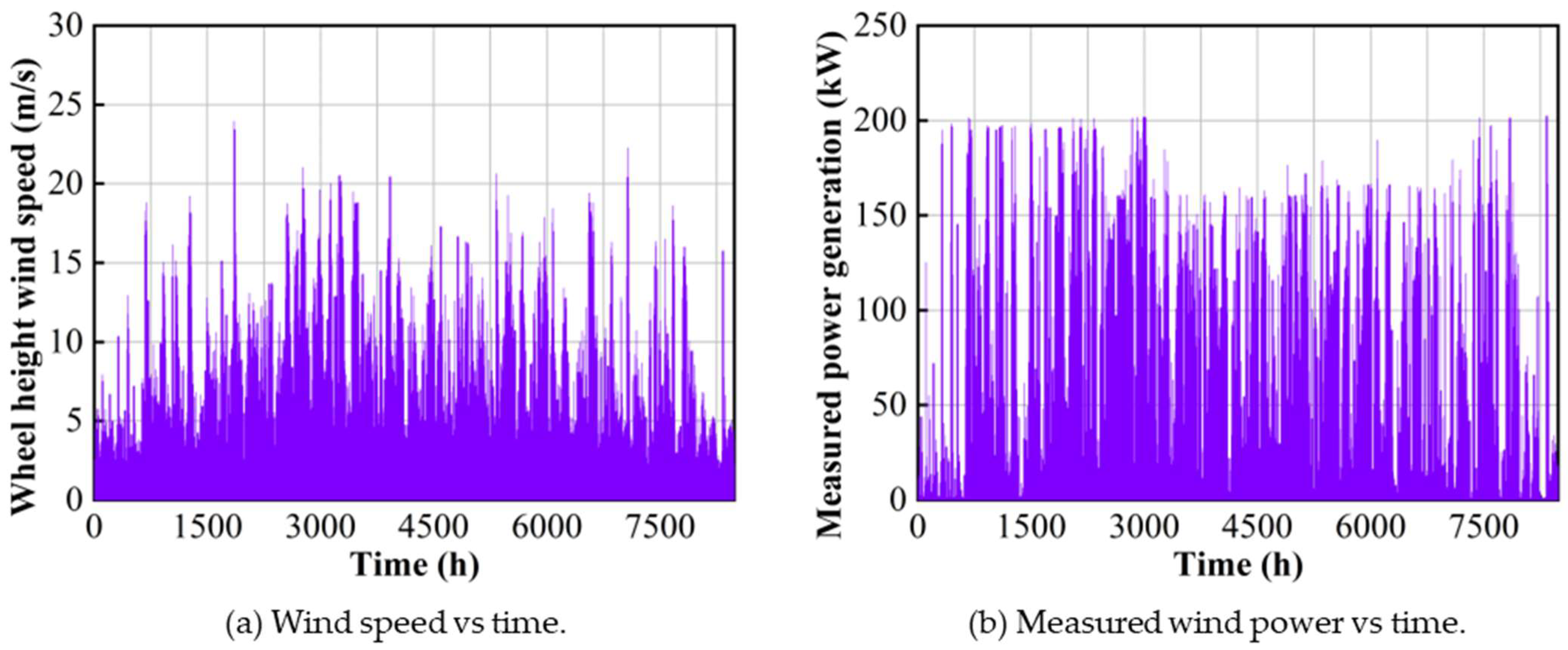
The data required for the deep learning prediction model include variables such as temperature, wind direction, air pressure, relative humidity, wind speed data, and wind power generation. In this study, real data from a wind farm in Xinjiang in 2019 were used for validation and prediction, and the data were collected at hourly intervals for a duration of one year from 1 January 2019 to 31 December 2019, thus accumulating a large dataset of 8760 observations.

Table 1. Symbols and statistical characteristics of the measured variables.

Atmospheric Variables	Notation	Max	Min
Temperature (℃)	Te	40.12	−18.21
Relative humidity (%)	RH	94.92	2.51
Atmospheric pressure (kPa)	AP	905.31	874.58
Wind direction (°)	WD	359.88	0.04
Wind speed (m/s)	WS	23.96	0.00
Wind power (kW)	WP	202.23	0.26

provides the symbols and statistical characteristics of the measured variables.

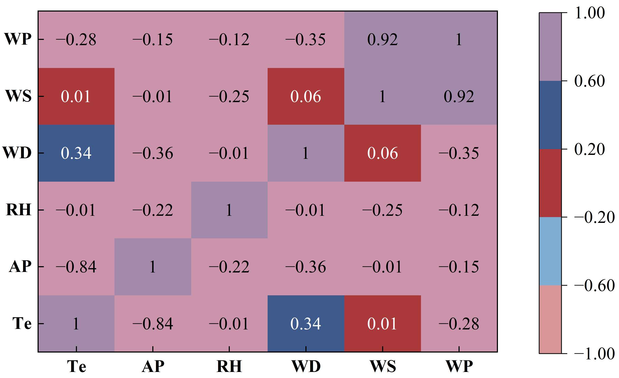
To check for potential interconnections between the variables, Pearson correlation coefficients of the variables were calculated as shown in Equation (62) and the experimental results were analysed. The results of the resulting correlation matrix are shown in Figure 5.

$$\mathrm{C}={\displaystyle \frac{{\displaystyle \sum _{\mathrm{t}=1}^{\mathrm{T}}}(\mathrm{x}(\mathrm{t})-\overline{\mathrm{x}})(\mathrm{y}(\mathrm{t})-\overline{\mathrm{y}})}{\sqrt{{\displaystyle \sum _{\mathrm{t}=1}^{\mathrm{T}}}{(\mathrm{x}(\mathrm{t})-\overline{\mathrm{x}})}^2{(\mathrm{y}(\mathrm{t})-\overline{\mathrm{y}})}^2}}}$$

(62)

where $\mathrm{x}(\mathrm{t})$ and $\mathrm{y}(\mathrm{t})$ are two arbitrary time series variables and $\overline{\mathrm{x}}$ and $\overline{\mathrm{y}}$ stand for the mean values of the sequences $\mathrm{x}(\mathrm{t})$ and $\mathrm{y}(\mathrm{t})$.

Figure 5 shows that there is a direct negative correlation between wind speed and relative humidity, with a coefficient value of −0.25. In addition, relative humidity is negatively correlated with atmospheric pressure. Furthermore, atmospheric pressure was positively correlated with all other atmospheric variables except wind speed, indicating an indirect relationship between these variables and wind speed. In addition, the coefficient value of wind speed and historical wind power output is 0.92, indicating an extremely important correlation between wind speed and wind power. Therefore, wind speed and historical wind power output are also important eigenvalues to be used as deep learning for the model. The wind speed data and wind power output data are shown in Figure 6a,b.

Since wind speed and wind power output data are continuous variables, the missing value treatment of the data used in this study uses linear interpolation to fill in the missing values by following the trend of neighbouring data points. The method is computationally simple, efficient, and suitable for real-time processing of large-scale data. The derivation of the formula for linear interpolation is based on the point-slope equation, as shown in Equation (63).

$$\mathrm{y}={\mathrm{y}}_0+{\displaystyle \frac{({\mathrm{y}}_1-{\mathrm{y}}_0)}{({\mathrm{x}}_1-{\mathrm{x}}_0)}}\cdot (\mathrm{x}-{\mathrm{x}}_0)$$

(63)

where ${\displaystyle \frac{({\mathrm{y}}_1-{\mathrm{y}}_0)}{({\mathrm{x}}_1-{\mathrm{x}}_0)}}$ denotes the rate of change between data points.

The Z-Score method is still required for outlier treatment of data after missing value treatment as used in this study. If the variable data follow a normal distribution, the mean deviation $\mu$ and standard deviation $\sigma$ of each variable are calculated, and data exceeding $\mu$ $\pm$3 $\sigma$ are considered outliers. When $\left|Z\right|$ > 3, the data is determined to be an outlier. This method can be used for the rapid detection of extreme values in the variables, and the calculation is simple, which can greatly improve the efficiency of data cleaning. The principle of the method is shown in Equation (64).

$$Z={\displaystyle \frac{x-\mu }{\sigma }}$$

(64)

To maintain data integrity and prevent information leakage, a temporal segmentation method was applied to the dataset. This process entails dividing the dataset into different subsets, allocating 80% for the training set, 15% for the validation set, and another 5% for the test set, as shown in

Table 2. The detail of dividing the data set.

Set	Number of Data	Ratio (%)
Training set	7008	80
Validation set	1314	15
Testing set	438	5
Total	8760	100

.

The model parameters are fine-tuned using the training set, while the hyperparameters are optimised using the validation set. This careful delineation and systematic utilisation of the different dataset components ensured a rigorous and unbiased assessment of the model’s generalisation capabilities. To facilitate model convergence during training, the eigenvalues were normalised as shown in Equation (65).

$${\mathrm{x}}_{\mathrm{i},\mathrm{j}}^{\mathrm{n}}={\displaystyle \frac{{\mathrm{x}}_{\mathrm{i},\mathrm{j}}-{\mathrm{x}}_{\mathrm{j},\mathrm{m}\mathrm{i}\mathrm{n}}}{{\mathrm{x}}_{\mathrm{j},\mathrm{m}\mathrm{a}\mathrm{x}}-{\mathrm{x}}_{\mathrm{j},\mathrm{m}\mathrm{i}\mathrm{n}}}}$$

(65)

where $\mathrm{n}$ represents normalisation operation, ${\mathrm{x}}_{\mathrm{i},\mathrm{j}}$ is the original feature value, and ${\mathrm{x}}_{\mathrm{j},\mathrm{m}\mathrm{i}\mathrm{n}}$ and ${\mathrm{x}}_{\mathrm{j},\mathrm{m}\mathrm{a}\mathrm{x}}$ are the global minimum and global maximum of the $\mathrm{j}$-th feature, respectively.

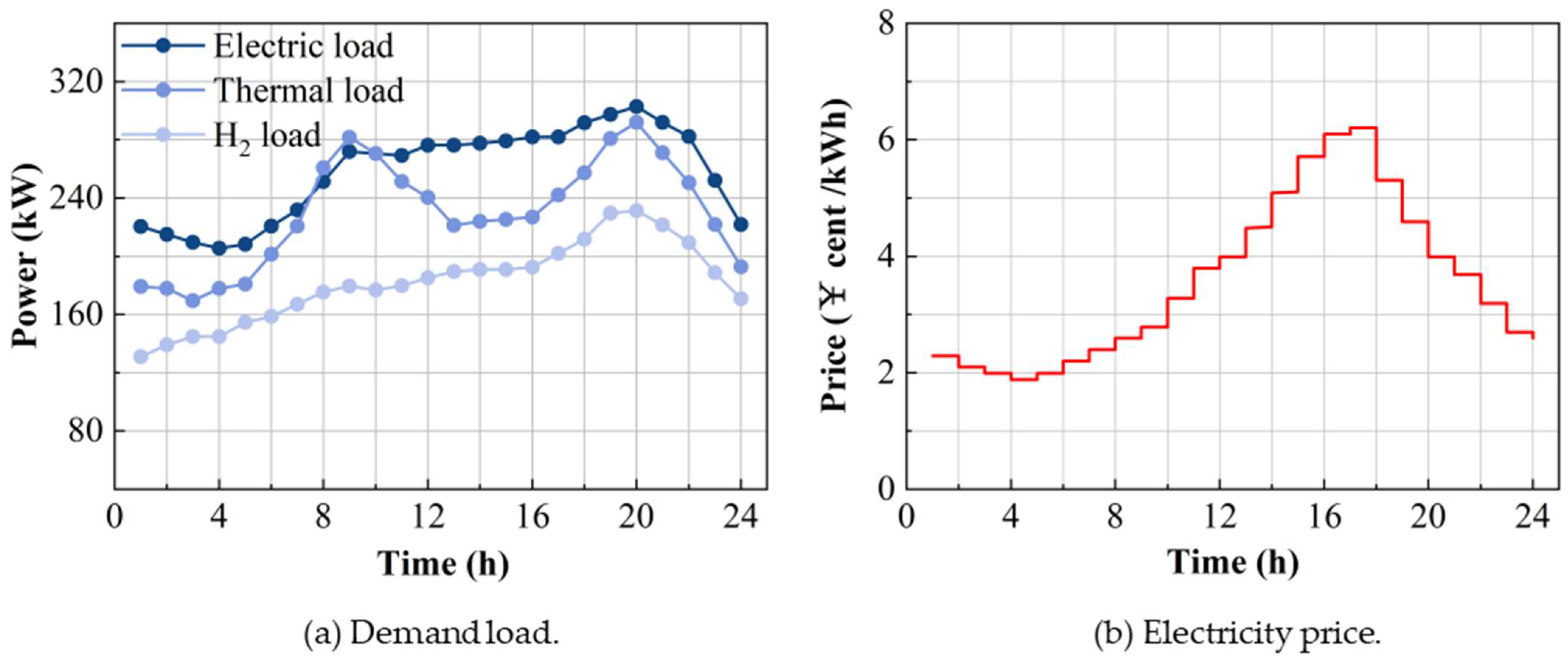
The electricity, heat, and hydrogen loads required by the microgrid in the optimisation model for each time of day are shown in Figure 7a. Figure 7b shows the results of the electricity price forecast for each day-ahead period.

4. Results and Discussion

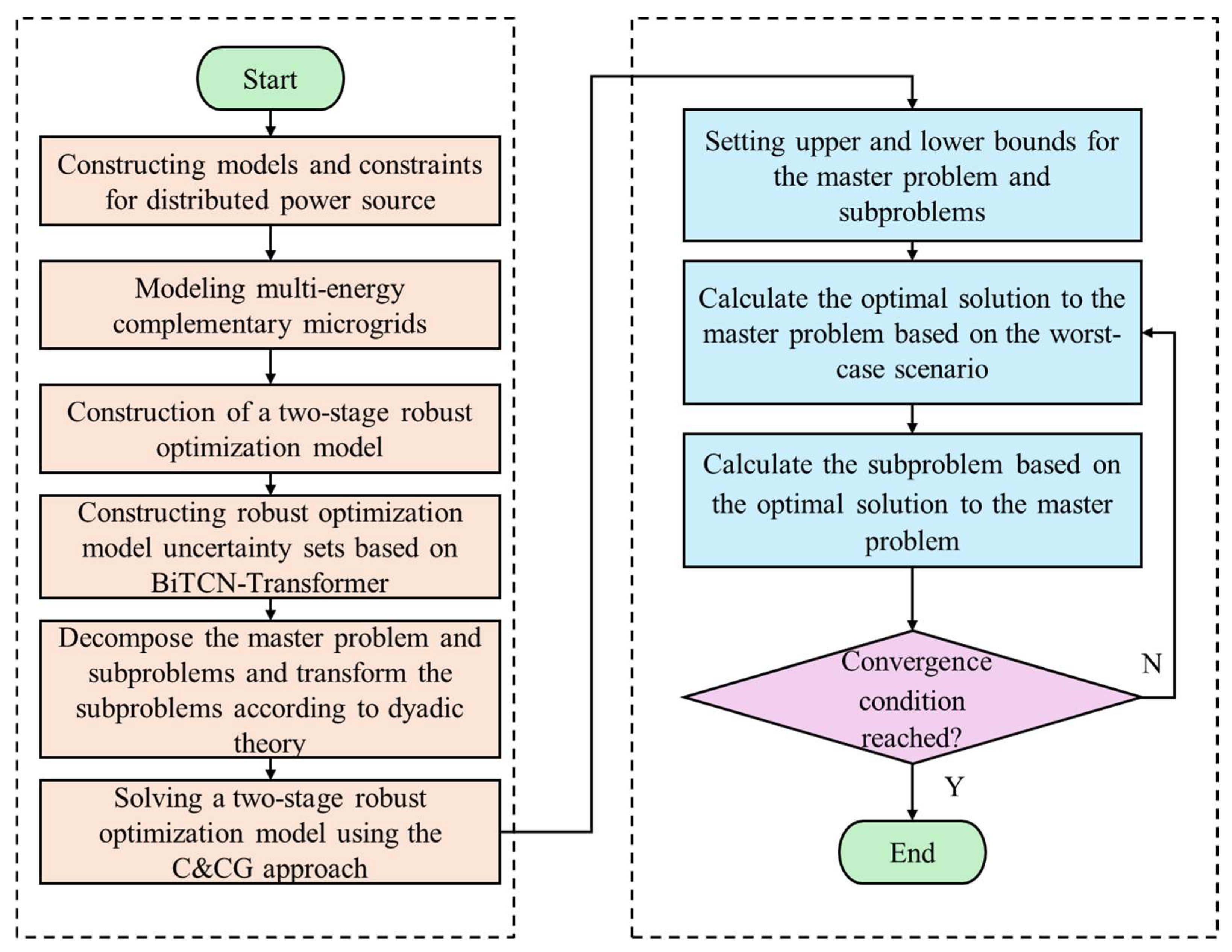
The effectiveness of the proposed prediction and optimisation models was verified through two sets of experiments. Historical wind speed and wind power generation data were used to conduct point prediction and ablation experiments for the deep learning model, with comparisons made against other advanced models through prediction result curves, regression plots, and evaluation metrics. Based on the point prediction results, interval prediction was performed using a kernel density model and confidence interval calculation method, with scenarios divided into high and low wind power output conditions. These two scenarios were employed to construct a robust optimisation box uncertainty set, followed by two-stage robust optimisation of the multi-energy complementary microgrid energy management model to analyse daily variations in electrical, thermal, and hydrogen loads along with carbon trading outcomes under both scenarios. The experiments were conducted in a computational environment consisting of a Windows 10 (8-core, 64-bit) operating system with a GeForce RTX 3080Ti GPU, using MATLAB R2023b for program execution.

4.1. Predictive Modelling Results

Deep learning point predictions are the basis of interval prediction, so to better construct the uncertainty set for two-stage robust optimisation, the predictive effectiveness of the proposed deep learning point predictions needs to be validated. Ablation experiments are an excellent method of validating the effectiveness of point prediction. Ablation experiments provide an effective means of evaluating the contribution and necessity of individual components in the model. By removing or replacing specific components or sub-models sequentially, a clearer picture of the impact of each part on the overall performance of the model can be obtained. This approach not only helps optimise the model structure but also helps deepen the understanding of its mechanisms. In this study, ablation experiments were conducted to verify the point prediction validity of the proposed predictive model.

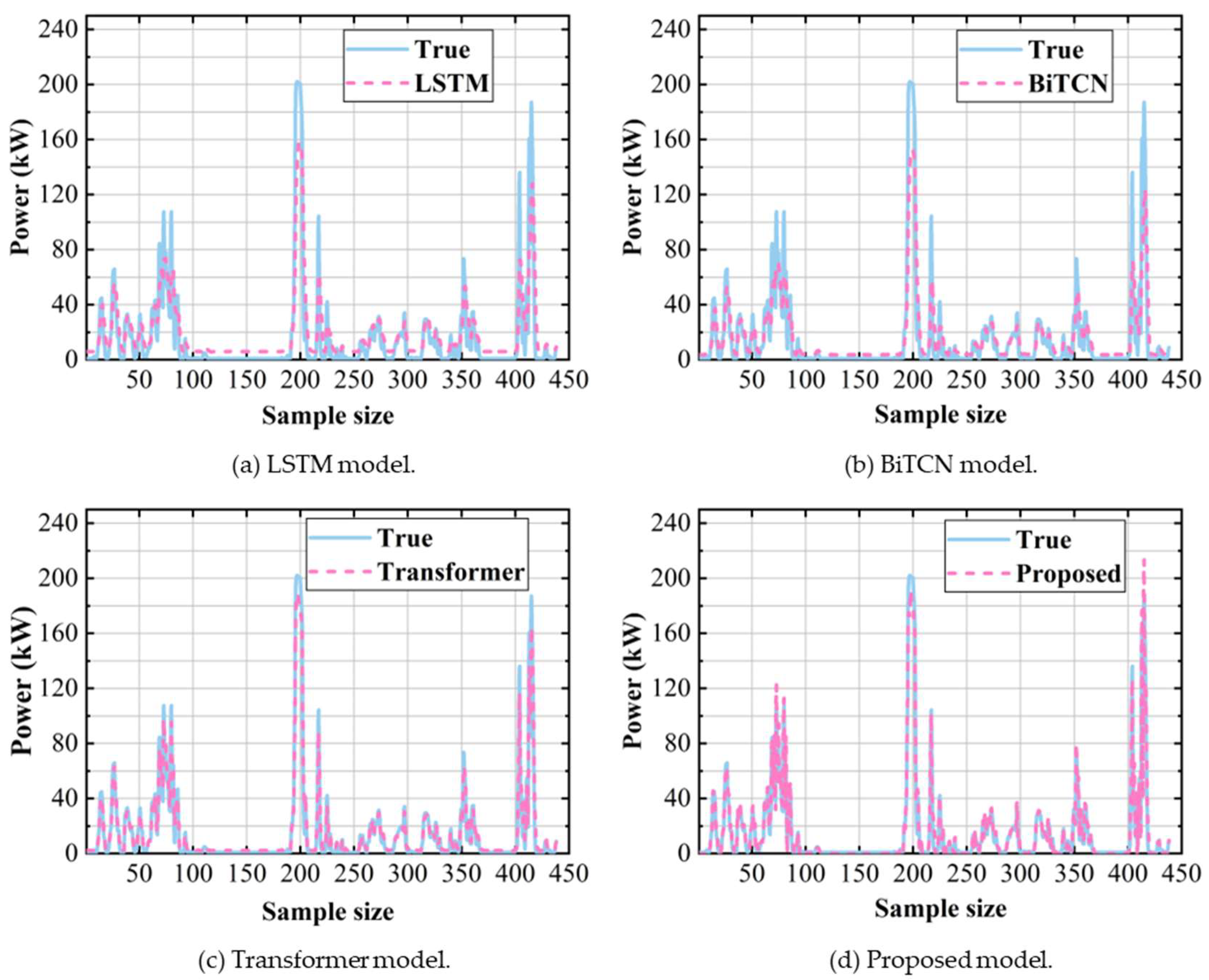
The dataset division of the ablation experiment is determined by Table 2, and the random seed is set to 35. The ablation experiment needs to systematically remove some of the components to analyse the roles of each part. Meanwhile, the LSTM, as a classical recurrent neural network, is commonly used to capture temporal dependencies, and it is a typical representative of the traditional recursive architecture. Therefore, the LSTM, BiTCN, and Transformer models were selected as the baseline models for the ablation experiments.

Figure 8 displays a comparison of the prediction results of LSTM, BiTCN, Transformer, and the proposed model. As shown in Figure 8, the tests with the proposed prediction model show better results in order, while the single-model LSTM has the biggest difference from the actual values. Both the BiTCN and Transformer models show improvements, but still have noticeable errors compared to the true values. The proposed model has the best fitting effect between the prediction results and the real values.

Table 3. The evaluation metrics of the ablation experiment.

	MAE	RMSE	R2
LSTM	1.7823	3.0156	0.9124
BiTCN	1.5039	2.6348	0.9427
Transformer	1.4015	2.5021	0.9583
Proposed	1.3512	2.4856	0.9683

displays the evaluation metrics of the ablation experiment model. As shown in Table 3, the quantitative data analysis reveals that the fitting ability of the LSTM model is limited. The reason for this limitation is that the LSTM model relies on a single model for time series modelling, while the lack of an attention mechanism and bidirectional temporal modelling capability leads to insufficient capture of local features, making it the weakest performer among the four model architectures.

After switching to the BiTCN model, the comprehensive performance of the model is improved. Its convolutional filter enhances the local feature extraction of wind speed and wind power sequences and realises multi-scale time series modelling. Compared with the LSTM model, the MAE of the BiTCN model is reduced by 15.6%, the RMSE is reduced by 12.6%, and the R² is improved by 3.3%.

The Transformer model incorporates an internal attention model, which can effectively extract local short-term fluctuations in wind and wind speed data and, at the same time, helps to understand different situations in time series data from multiple perspectives. This implementation greatly reduces the error and improves the fitting ability. Compared to the BiTCN model, the MAE is reduced by 5.8%, the RMSE is reduced by 4.4%, and R² is improved by 1.7%.

By integrating the BiTCN model and the Transformer model into the BiTCN-Transformer framework, this integration improves the performance of the model in terms of feature extraction and global dependency of wind data. The simulation results indicate that the proposed model further reduces the MAE by 2.8%, RMSE by 0.6%, and R² by 1.2% compared to the Transformer model.

Table 4. Comparison of the evaluation results with other models.

	MAE	RMSE	R2	Computation Time (s)
CNN-LSTM	1.6928	2.9123	0.9521	92
Informer	1.3985	2.4810	0.9852	145
VMD-CNN-BiLSTM	1.2687	2.3515	0.9734	210
Proposed	1.3512	2.4856	0.9683	68

shows the results of the evaluation metrics of the proposed model compared with other state-of-the-art prediction models for wind power prediction. Other models include CNN-LSTM [34], Informer [35], and VMD-CNN-BiLSTM [36].

In terms of comprehensive performance, the proposed model achieves a remarkable balance between prediction accuracy and computational efficiency. Compared with CNN-LSTM, its MAE and RMSE are reduced by 29.7% and 33.0%, respectively, R² is improved by 3.98%, and the single training time is only 68 s, which is 26.1% shorter than the 92 s of CNN-LSTM. This advantage is attributed to BiTCN’s bidirectional temporal convolution module, which significantly improves computational efficiency by replacing the serial LSTM structure in CNN-LSTM with parallelised feature extraction.

Although the R² of the Informer model is slightly better than that of the proposed model, its computation time is 2.13 times that of the latter and its MAE and RMSE are higher than that of the proposed model. This indicates that although the global self-attention mechanism relied on by Informer can capture long sequence dependencies, it has high computational complexity and is difficult to adapt to real-time prediction needs. On the other hand, BiTCN-Transformer, through the synergistic design of local dilation convolution and a lightweight attention module, ensures the time-series modelling capability while considering the accuracy and efficiency.

It is worth noting that the MAE and RMSE of VMD-CNN-BiLSTM are slightly better than the proposed model, but its operation time is 3.09 times longer than that of the proposed model and its R² is lower than that of the proposed model. This is because VMD-CNN-BiLSTM needs to perform variational modal decomposition preprocessing superimposed on the time-series iterative computation of bidirectional LSTM, which leads to a surge in model complexity. In contrast, BiTCN-Transformer avoids the error accumulation problem of signal decomposition by joint bidirectional convolution-attention modeming.

4.2. Interval Prediction Results

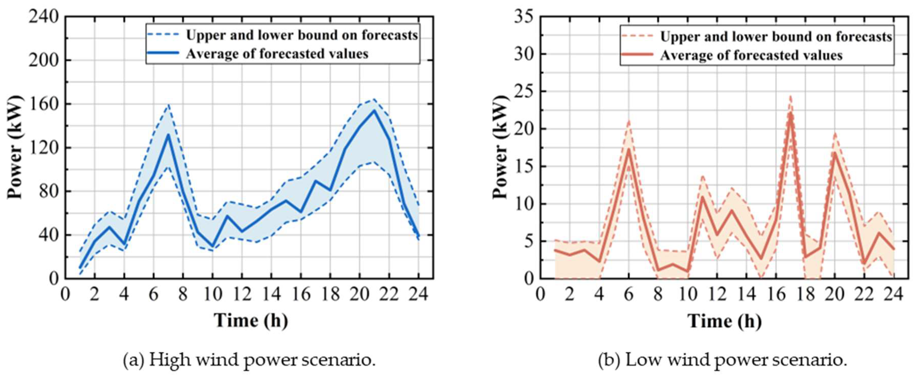
To establish the uncertainty set of the robust optimisation model, predicting the interval of wind power output is necessary; the upper and lower bounds of the intervals define the limits of the uncertainty set in the robust optimisation framework. In this study, interval prediction was performed for two scenarios, a high wind power scenario and a low wind power scenario, and the kernel density estimation method was used to fit the point predictions of the proposed deep learning model to obtain the interval prediction of wind power under the corresponding confidence intervals.

The wind power prediction intervals need to meet the grid dispatch’s demand for fault tolerance for extreme errors. In this study, a 90% confidence level was chosen to meet the reliability requirements of the IEC 61400-25 standard [37] for wind power prediction. The wind power interval prediction for both scenarios was performed based on the kernel density estimation model and the point prediction results of the proposed deep learning model, as shown in Figure 9. Interval prediction not only requires the construction of clear upper and lower bounds, but also necessitates an analysis of the results with evaluation indicators. In this study, two evaluations of the prediction results under two different scenarios, PICP and CWC, were conducted to verify the effectiveness of the proposed model in interval prediction, as shown in

Table 5. Evaluation indicators for interval prediction.

Scenario	Evaluation Indicators	Numerical Value
High Wind Power Scenario	PICP	0.91
	CWC	1.89
Low Wind Power Scenario	PICP	0.93
	CWC	0.76

. As illustrated in Table 5, the PICP and CWC of the proposed model interval prediction in the two scenarios are within a good range of values, which indicates that the proposed model can consider the balance between robustness and economy in constructing the uncertainty set in a good way.

4.3. Optimisation Modelling Results

The outcomes of the data interval predictions are used to build the uncertainty set for the two-stage robust optimisation model. To determine the changes in electrical energy demand, thermal energy load, hydrogen energy load, and findings pertaining to carbon trading for each of the two wind power scenarios, the model was solved using Matlab software (R2023b).

The results of the optimisation for the high-wind power scenario are displayed in Figure 10. Figure 10 shows that:

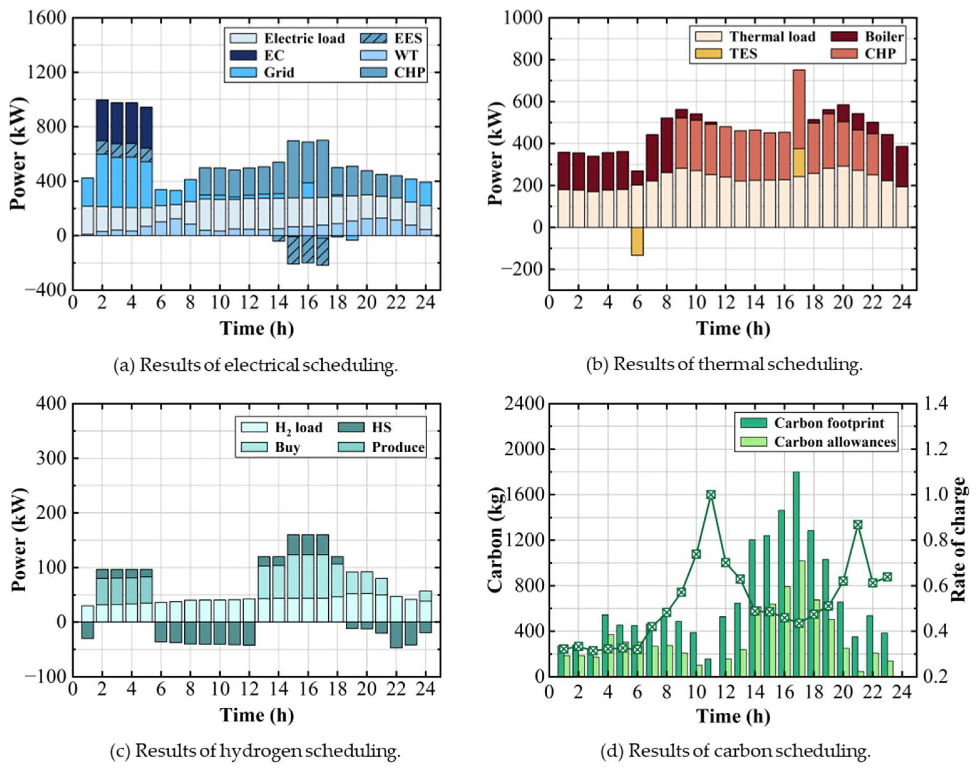
As shown in Figure 10a, in the result of energy management of electric power load, in the low tariff period (2–5 h), the wind power output is low (31.6–69.2 kW), which is not enough to support the electric power demand of the electric load (206–214 kW) and electrolyser. At the same time, the purchased power is increased to 136–483 kW. At this time, the cost of hydrogen production is lowest, the EES is charged with a constant power of 100 kW, and the EC is charged at a full power of 300 kW. During the high tariff stage (15–17 h), the output of wind power increases. During this time, the highest amount of power from the CHP system (420 kW) and EES discharge (200 kW) can be sold to the grid (207 kW) by combining the CHP gas power generation and the storage system discharge to maximise profit during peak hours. In the CHP start-stop control phase (9–22 h), it is activated in the rising electricity price phase. The output is dynamically adjusted according to the demand of the thermoelectric coupling and the electricity/heat ratio is set at 1:1.2 to realise the energy ladder utilisation.

Figure 10b shows that during the thermal electrolytic coupling period (6 h), the thermal load increases to 200 kW in the morning peak, but the CHP system has not yet been activated. The TES system releases 133.53 kW of stored heat, and the boiler only needs to provide 66.64 kW to reduce gas consumption. During the CHP waste heat excess phase (17 h), the CHP generates 504 kW of waste heat due to power supply demand, which significantly exceeds the current heat load limit. Therefore, the TES stores 146.30 kW of heat to prevent waste and reserve it for future heat supply. In the CHP–boiler combined operation stage (20 h), the boiler supplements the 78.94 kW load, realising the economic operation mode of “CHP + boiler peaking”.

Figure 10c shows that between 2 and 5 h, EC makes hydrogen at its maximum rate of 48.24 kg/h during the cheaper tariff time, producing more hydrogen than needed and storing 63.8 kg of HS, which helps cover costs later when tariffs are higher. In the hydrogen purchase–storage phase (15–17 h), hydrogen production is stopped during the peak tariff period, and the demand is met by hydrogen purchases, while HS is storing hydrogen to smooth out the cost fluctuation caused by hydrogen purchases.

Figure 10d shows renewable energy contributions to a higher value of carbon emissions due to the higher amount of wind power and therefore a higher utilisation of carbon allowances.

The optimisation results for the low-wind power scenario are shown in Figure 11.

As illustrated in Figure 11a, in terms of the electrical energy management results, during the low tariff period (2–5 h), the wind power output is 0.8–8 kW, only 2.5% of the high wind power scenario, at which time the EC is shut down due to the lack of wind power to produce hydrogen, and the amount of hydrogen purchased is increased to 80 kg/h. The charging of the EES is limited as a result. In the high tariff phase (15–17 h), when the wind power output grows slightly and the CHP system is overloaded, the EES is discharged at 200 kW, and the revenue from electricity sales is reduced due to the decreased efficiency of the CHP system.

Figure 11b shows the CHP waste heat utilisation rate continues to improve compared to the high wind power scenario, and continuous CHP work is achieved for 9–17 h. TES completes the heat storage of 480.5 kW from 1–8 h and releases heat storage of 460.2 kW from 14–17 h, smoothing out the deviation between the CHP heat output and the load demand. At the same time, the boiler continues to operate.

Figure 11c reveals that a completed EC shutdown leads to a complete interruption of hydrogen production and full-time dependence on hydrogen purchases. In addition, the HS function is reversed: 1–5 h mandatory HS (hydrogen purchases are greater than the load) and 19–21 h continuous discharge from the tanks, which triggers the risk of a hydrogen energy shortage.

Figure 11d shows that due to the extremely low wind power output, the value of renewable energy contributing to carbon emissions is also extremely low, the carbon quota gap is huge, and a larger carbon cost needs to be paid, which makes the overall operation cost higher.

The results of microgrid optimisation for both high and low wind power scenarios show that the DGs within the microgrid in the low wind power scenario are increased relative to the high wind power scenario, indicating that the proposed microgrid optimisation model can still achieve the lowest cost within the system in the case of insufficient access to renewable energy sources, which verifies the validity and reliability of the proposed model.

4.4. Economic Analysis

An economic analysis is needed to visually compare the difference in microgrid costs between the high-wind and low-wind scenarios through a cost evaluation.

Table 6. Comparison of cost indicators.

	High Wind Power Scenario	Low Wind Power Scenario	Rate of Change (%)
Total Cost (¥)	15,954	61,139	283
Percentage of Purchased Electricity Cost (%)	17.6	20.6	17
Percentage of Hydrogen Purchase Cost (%)	22.6	20	−11.5
Electricity Sales Revenue (¥)	2235	1680	−24.8
Hydrogen Unit Cost (¥/kg)	8.2	10.0	21.9
Carbon Emission Cost (¥)	7650	31,703	314

shows the comparison of cost indicators, such as total cost as well as carbon emission cost, for both scenarios.

As displayed in Table 6 and the comparison of load dispatching power in the high and low wind power scenarios, the total system cost in the low wind power scenario increases by 283%, the cost of carbon emissions increases by 314%, the revenue from electricity sales decreases by 24.8%, and the cost of the HS system increases by 21.9%. This happens because in the high wind power scenario, the microgrid system lowers costs and carbon emissions by effectively using wind power, energy storage, hydrogen production, and heat storage together. However, in the low wind power scenario, the system relies more on buying power and hydrogen, leading to higher carbon emissions due to not enough renewable energy being available. In addition, in the high wind scenario, the tariff difference triggers the arbitrage behaviour of electric storage, which can significantly reduce the total system cost. In the low wind scenario, the tariff mechanism fails, the CHP system is overloaded, and the cost of the generation unit increases significantly.

In a high wind power scenario, wind energy output can substantially decrease system carbon emissions. Conversely, in a low wind power scenario, inadequate wind energy necessitates the use of hydrogen fuel cells for operation, thereby increasing the system’s carbon emissions. The microgrid model proposed in this work can modulate the output of each component to maintain system operation according to the fluctuating availability of renewable energy. However, a significant proportion of renewable energy is essential to reducing costs and carbon emissions within the microgrid system, and enhancing energy management in challenging circumstances necessitates improved resilience in system design.

4.5. Robust Parameter Sensitivity Analysis

The uncertainty parameter $\mathsf{\Gamma }$ represents the maximum relative deviation allowed for wind power output from the midpoint of the uncertainty set interval. Changes in $\mathsf{\Gamma }$ significantly impact cost scheduling outcomes. When $\mathsf{\Gamma }$ is 0, wind power output strictly equals the midpoint of the forecasted interval, meaning no fluctuation. When $\mathsf{\Gamma }$ is 0.5, wind power output can reach the original upper and lower bounds of the forecasted interval. Thus, the mathematically valid range for $\mathsf{\Gamma }$ is [0, 0.5]. 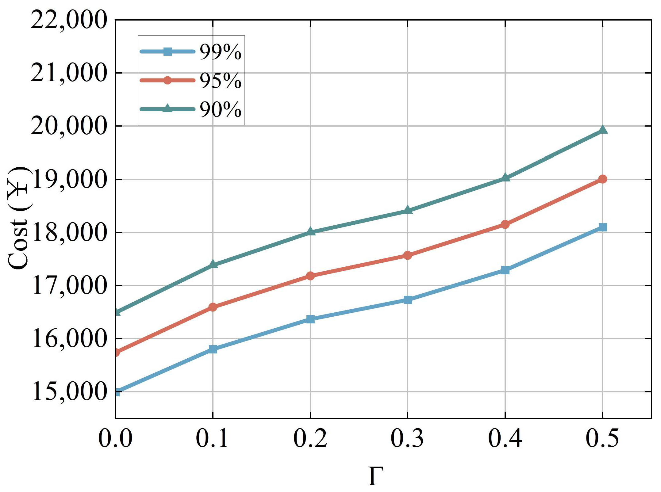Figure 12 shows the total system cost variation as $\mathsf{\Gamma }$ increases from 0 to 0.5 under confidence intervals of 90%, 95%, and 99%.

From Figure 12, it is noted that a larger $\mathsf{\Gamma }$ value corresponds to a wider range of wind power fluctuations, requiring the system to account for greater uncertainty. To address these expanded uncertainty scenarios, additional equipment such as gas turbines and HS must compensate, leading to higher system costs as $\mathsf{\Gamma }$ increases. When $\mathsf{\Gamma }$ is in the range of [0, 0.3], the system cost rises gradually, because minor adjustments by backup equipment can offset the increased costs caused by moderate uncertainty. However, when $\mathsf{\Gamma }$ is within [0.3, 0.5], the cost increases more sharply. This is due to efficiency losses in the CHP system and frequent charging/discharging cycles of HS, which become insufficient to manage the heightened uncertainty. As a result, costs escalate further, indicating that moderate $\mathsf{\Gamma }$ values strike a balance between system robustness and economic efficiency. Additionally, the size of the confidence interval directly impacts total costs. For a fixed $\mathsf{\Gamma }$, expanding the confidence interval widens the predicted wind power range, forcing the system to prepare for more extreme scenarios. This necessitates greater resource reserves, further driving up costs.

5. Conclusions and Future Directions

The uncertainty of renewable energy output greatly affects the stability of microgrid optimisation operations. A strong optimisation model for a multi-energy complementary microgrid that includes carbon trading is proposed here, and the BiTCN-Transformer model is used to make deep learning predictions in two common scenarios—one with a lot of wind power and one with little wind power—to build the uncertainty set for the robust optimisation model. Simulation and comparison experiments are carried out. This article summarises the main work, as follows:

(a) A comprehensive optimisation model is presented for a multi-energy complementary microgrid that integrates electricity, heat, gas, and hydrogen and incorporates a carbon trading mechanism. The multi-energy complementary microgrid model improves how different power sources work together, helping to smooth out changes in energy demand and making sure the microgrid runs steadily and reliably.

(b) We propose a wind power point prediction method based on the BiTCN-Transformer deep learning model, which utilises a nonparametric kernel density model and confidence intervals to construct interval prediction results from deep learning, thereby establishing a box uncertainty set for the robust optimisation model.

(c) The proposed multi-energy complementary microgrid model for electricity, heat, gas, and hydrogen demonstrates considerable benefits in both high- and low-wind-power scenarios. This situation underscores that the integration of a significant proportion of renewable energy is essential for the smooth and efficient operation and management of the microgrid.

(d) Economic analysis demonstrates that microgrid operation under high- and low-wind-power scenarios differs. In the low wind scenario, the total system cost climbs 283% (2.8 times), carbon emission costs rise 314%, power sales revenue drops 24.8%, and HS system costs jump 21.9%. The analysis shows that a high renewable energy penetration is still essential for system cost reduction and efficiency.

(e) The proposed predictive model relies on the variability of wind power and wind speed data from the preceding year. Future models such as GAN can directly generate future wind power output data and establish robust optimisation model uncertainty sets. The suggested model for microgrid energy management can incorporate more renewable energy sources, such as solar power generation, to improve the microgrid’s capacity for renewable energy consumption. Meanwhile, model-free reinforcement learning methods, as an emerging approach in microgrid energy management, can achieve desired results and should be prioritised in future research.

References

1. Dey, B.; Misra, S.; Chhualsingh, T.; Sahoo, A.K.; Singh, A.R. A hybrid metaheuristic approach to solve grid centric cleaner economic energy management of microgrid systems. J. Clean. Prod. 2024, 448, 141311. [Google Scholar] [CrossRef]
2. Kyriakou, D.G.; Kanellos, F.D.; Tsekouras, G.J.; Moungos, K.A. Effective and Local Constraint-Aware Load Shifting for Microgrid-Based Energy Communities. Energies 2025, 18, 343. [Google Scholar] [CrossRef]
3. Ahmadi Jirdehi, M.; Shaterabadi, M.; Sohrabi Tabar, V.; Rezaee Jordehi, A. Impact of diverse penetration levels of thermal units on a hybrid microgrid energy management considering the time of use and function priority. Appl. Therm. Eng. 2022, 217, 119164. [Google Scholar] [CrossRef]
4. Wang, Y.; Wang, Z.; Sheng, H. Optimizing wind turbine integration in microgrids through enhanced multi-control of energy storage and micro-resources for enhanced stability. J. Clean. Prod. 2024, 444, 140965. [Google Scholar] [CrossRef]
5. Cheng, H.; Liao, X.; Li, H.; Lü, Q. Dynamic-Based Privacy Preservation for Distributed Economic Dispatch of Microgrids. IEEE Trans. Control Netw. Syst. 2025, 12, 1029–1039. [Google Scholar] [CrossRef]
6. Jiao, X.; Zhang, D.; Zhang, Z.; Yin, R.; Wang, L.; Zhu, C.; Nie, F. A Hybrid Deep and Broad Learning Architecture for Wind Power Forecasting Based on Spatial–Temporal Feature Selection. IEEE Trans. Instrum. Meas. 2025, 74 Pt C, 2510416. [Google Scholar] [CrossRef]
7. Xiang, X.; Li, X.; Zhang, Y.; Hu, J. A short-term forecasting method for photovoltaic power generation based on the TCN-ECANet-GRU hybrid model. Sci. Rep. 2024, 14, 6744. [Google Scholar] [CrossRef]
8. Zhang, D.; Chen, B.; Zhu, H.; Goh, H.H.; Dong, Y.; Wu, T. Short-term wind power prediction based on two-layer decomposition and BiTCN-BiLSTM-attention model. Energy 2023, 285, 128762. [Google Scholar] [CrossRef]
9. Shao, Z.; Han, J.; Zhao, W.; Zhou, K.; Yang, S. Hybrid model for short-term wind power forecasting based on singular spectrum analysis and a temporal convolutional attention network with an adaptive receptive field. Energy Convers. Manag. 2022, 269 (Suppl. C), 116138. [Google Scholar] [CrossRef]
10. Graves, A.; Schmidhuber, J. Framewise phoneme classification with bidirectional LSTM and other neural network architectures. Neural Netw. Off. J. Int. Neural Netw. Soc. 2005, 18, 602–610. [Google Scholar] [CrossRef]
11. Limouni, T.; Yaagoubi, R.; Bouziane, K.; Guissi, K.; Baali, E.H. Accurate one step and multistep forecasting of very short-term PV power using LSTM-TCN model. Renew. Energy 2023, 205, 1010–1024. [Google Scholar] [CrossRef]
12. Liu, W.; Mao, Z. Short-term photovoltaic power forecasting with feature extraction and attention mechanisms. Renew. Energy 2024, 226, 120437. [Google Scholar] [CrossRef]
13. Cheng, J.; Luo, X.; Jin, Z. Integrating domain knowledge into transformer for short-term wind power forecasting. Energy 2024, 312, 133511. [Google Scholar] [CrossRef]
14. Chen, J.; Zhao, Y.; Wang, M.; Yang, K.; Ge, Y.; Wang, K.; Lin, H.; Pan, P.; Hu, H.; He, Z.; et al. Multi-timescale Reward-based DRL Energy Management for Regenerative Braking Energy Storage System. IEEE Trans. Transp. Electrif. 2025, 99, 1. [Google Scholar] [CrossRef]
15. Zhao, C.; Li, Y.; Zhang, Q.; Ren, L. Low Carbon Economic Energy Management Method in a Microgrid Based on Enhanced D3QN Algorithm with Mixed Penalty Function. IEEE Trans. Sustain. Energy 2025, 15, 1–11. [Google Scholar] [CrossRef]
16. Diao, X.; Song, Y.; Sahoo, S.; Li, Y. Neuromorphic Event-Driven Semantic Communication in Microgrids. IEEE Trans. Smart Grid 2024, 15, 1. [Google Scholar] [CrossRef]
17. Fan, W.; Ju, L.; Tan, Z.; Li, X.; Zhang, A.; Li, X.; Wang, Y. Two-stage distributionally robust optimization model of integrated energy system group considering energy sharing and carbon transfer. Appl. Energy 2023, 331, 120426. [Google Scholar] [CrossRef]
18. Li, Y.; Han, M.; Shahidehpour, M.; Li, J.; Long, C. Data-driven distributionally robust scheduling of community integrated energy systems with uncertain renewable generations considering integrated demand response. Appl. Energy 2023, 335, 120749. [Google Scholar] [CrossRef]
19. Ma, M.; Long, Z.; Liu, X.; Lee, K.Y. Distributionally robust optimization of electric–thermal–hydrogen integrated energy system considering source–load uncertainty. Energy 2025, 316, 134568. [Google Scholar] [CrossRef]
20. Yang, M.; Wang, J.; Chen, Y.; Zeng, Y.; Su, X. Data-driven robust optimization scheduling for microgrid day-ahead to intra-day operations based on renewable energy interval prediction. Energy 2024, 313, 134058. [Google Scholar] [CrossRef]
21. Zhu, X.; Zeng, B.; Dong, H.; Liu, J. An interval-prediction based robust optimization approach for energy-hub operation scheduling considering flexible ramping products. Energy 2020, 194, 116821. [Google Scholar] [CrossRef]
22. Xu, Y.; Wang, Y.; Liu, C.; Xiong, J.; Zhou, M.; Du, Y. Adaptive Robust Optimal Scheduling of Combined Heat and Power Microgrids Based on Photovoltaic Mechanism/Data Fusion-Driven Power Prediction. Energies 2025, 18, 732. [Google Scholar] [CrossRef]
23. Chen, F.; Lei, J.; Liu, Z.; Xiong, X. A Comparative Study on the Average CO2 Emission Factors of Electricity of China. Energies 2025, 18, 654. [Google Scholar] [CrossRef]
24. Kohút, R.; Klaučo, M.; Kvasnica, M. Unified carbon emissions and market prices forecasts of the power grid. Appl. Energy 2025, 377, 124527. [Google Scholar] [CrossRef]
25. Schmidhalter, I.; Mussati, M.C.; Mussati, S.F.; Oliva, D.G.; Fuentes, M.; Aguirre, P.A. Green hydrogen levelized cost assessment from wind energy in Argentina with dispatch constraints. Int. J. Hydrogen Energy 2024, 53, 1083–1096. [Google Scholar] [CrossRef]
26. Hu, J.; Ye, Y.; Wu, Y.; Zhao, P.; Liu, L. Rethinking Safe Policy Learning for Complex Constraints Satisfaction: A Glimpse in Real-Time Security Constrained Economic Dispatch Integrating Energy Storage Units. IEEE Trans. Power Syst. 2025, 40, 1091–1104. [Google Scholar] [CrossRef]
27. Shen, Z.; Wu, C.; Wang, L.; Zhang, G. Real-Time Energy Management for Microgrid with EV Station and CHP Generation. IEEE Trans. Netw. Sci. Eng. 2021, 8, 1492–1501. [Google Scholar] [CrossRef]
28. McAllister, R.D.; Esfahani, P.M. Distributionally Robust Model Predictive Control: Closed-loop Guarantees and Scalable Algorithms. IEEE Trans. Autom. Control 2024, 70, 2963–2978. [Google Scholar] [CrossRef]
29. Habib, S.; El-Ferik, S.; Gulzar, M.M.; Chauhdary, S.T.; Ahmad, H.; Ahmed, E.M. Optimizing integrated energy systems with a robust MISOCP model and C&CG algorithm for enhanced grid efficiency and profitability. Energy 2025, 318, 134795. [Google Scholar]
30. Hua, Z.; Yang, Q.; Chen, J.; Lan, T.; Zhao, D.; Dou, M.; Liang, B. Degradation prediction of PEMFC based on BiTCN-BiGRU-ELM fusion prognostic method. Int. J. Hydrogen Energy 2024, 87, 361–372. [Google Scholar] [CrossRef]
31. Jiang, W.; Liu, B.; Liang, Y.; Gao, H.; Lin, P.; Zhang, D.; Hu, G. Applicability analysis of transformer to wind speed forecasting by a novel deep learning framework with multiple atmospheric variables. Appl. Energy 2024, 353, 122155. [Google Scholar] [CrossRef]
32. Rao, Z.; Wang, K.; Tan, J.; Li, J.; Yang, Z.; Meng, W. Non-parametric Kernel Density Estimation and Analysis of Guangdong Offshore Wind Power Output Based on Optimal Bandwidth. Taiyangneng Xuebao/Acta Energiae Solaris Sin. 2023, 44, 274–282. [Google Scholar]
33. Shaojian, S.; Yiyuan, J.; Bin, L. Improved TCN model and its application in short-term photovoltaic power interval prediction. Appl. Res. Comput./Jisuanji Yingyong Yanjiu 2023, 40, 3064–3069. [Google Scholar]
34. Maślak, G.; Orłowski, P. A robust energy flow predictor based on CNN-LSTM for prosumer-oriented microgrids considering changes in biogas generation. Energy 2025, 326, 136050. [Google Scholar] [CrossRef]
35. Ma, Z.; Jiang, G.; Hu, Y.; Chen, J. A review of physics-informed machine learning for building energy modeling. Appl. Energy 2025, 381, 125169. [Google Scholar] [CrossRef]
36. Wang, D.; Li, S.; Fu, X. Short-Term Power Load Forecasting Based on Secondary Cleaning and CNN-BILSTM-Attention. Energies 2024, 17, 4142. [Google Scholar] [CrossRef]
37. Lee, J.-K.; Kim, D.-W.; Kim, S.-T.; Chae, C.-H.; Park, J.-Y. Development of Wind Turbine Simulation System Based on IEC 61400-25 Standard. KEPCO J. Electr. Power Energy 2019, 5, 349–359. [Google Scholar]
Figure 1. System architecture flowchart.
Energies 18 03111 g001
Figure 2. Two-stage robust model solution process flowchart.
Energies 18 03111 g002
Figure 3. The residual block structure in BiTCN.
Energies 18 03111 g003
Figure 4. The framework of Transformer model.
Energies 18 03111 g004
Figure 5. Pearson correlation coefficients of multiple atmospheric variables.
Energies 18 03111 g005
Figure 6. Wind speed and Measured wind power as a function of time: (a) Wind speed data; (b) Wind power data.
Energies 18 03111 g006
Figure 7. Demand load and electricity price data: (a) Demand load; (b) Electricity price.
Energies 18 03111 g007
Figure 8. Comparison of the predicted results: (a) Results of LSTM model; (b) Results of BiTCN model; (c) Results of Transformer model; (d) Results of proposed model.
Energies 18 03111 g008
Figure 9. Interval prediction results: (a) High wind power scenario; (b) Low wind power scenario.
Energies 18 03111 g009
Figure 10. Optimisation results for the high wind power scenario: (a) Results of electrical scheduling; (b) Results of thermal scheduling; (c) Results of hydrogen scheduling; (d) Results of carbon scheduling.
Energies 18 03111 g010
Figure 11. Optimisation results for the low wind power scenario: (a) Results of electrical scheduling; (b) Results of thermal scheduling; (c) Results of hydrogen scheduling; (d) Results of carbon scheduling.
Energies 18 03111 g011
Figure 12. Impact of robust parameter changes on total cost with different confidence intervals.
Energies 18 03111 g012