The Environmental Dimension of Sustainable Development in Relation to the Transition from Brown to Green Energy—A Case Study of Poland from 2005 to 2023

Abstract

The transition of the energy sector to green energy is one of the priorities of sustainable development, serving as an important instrument for balancing economic growth and environmental protection. The purpose of this article is to analyze the relationship between the share of renewable energy in total electricity production and the Environmental Dimension of Sustainable Development in the voivodeships of Poland during the years 2005–2023. To avoid difficulties in interpreting the statistical model—arising from challenges in determining the precise nature of the relationship between individual explanatory variables and the dependent variable—a collinearity test (using the Variance Inflation Factor, VIF, in three stages) was conducted. The relationship was examined using various statistical methods, including Pearson’s linear correlation and linear regression. Additionally, to visualize the local variation in this relationship, a spatial variation study was carried out using Geographic Information System (GIS) tools, supported by a series of bivariate choropleth maps. The results may suggest a positive impact of an increase in the share of electricity production from renewable energy sources on the state of the environment; however, this finding requires further, more detailed research.

1. Introduction

Climate change—including global warming and extreme weather events—is increasingly affecting the functioning of communities around the world [1,2,3]. In response, various environmental policies are being implemented, aimed at, among other things, transitioning from brown energy to green energy focused on achieving carbon neutrality worldwide [4,5,6]. Brown energy, generated from fossil fuels, is costly and significantly contributes to global warming [7]. Higher energy consumption results in increased energy costs and carbon emissions [8]. Climate change, along with environmental degradation and depletion of natural resources, is forcing policymakers worldwide to take action toward a transition to efficient and environmentally friendly energy solutions as quickly as possible [9,10,11,12,13]. As a result, achieving carbon neutrality has become one of the most important goals of the global energy transition. Energy efficiency and investment in renewable energy have even become key tools in policy-making [14,15,16]. From a global perspective, the urgent need to shift toward renewable energy sources has been recognized as essential for mitigating climate change [17,18,19,20,21].

Transitioning from brown energy to green energy is one of the primary development goals of the European Union. According to the “FIT for 55” initiative [22], investments in clean energy are planned, associated with an increase in funding for innovative projects and infrastructure to decarbonize industry. The green economy is epitomized by the “FIT for 55” initiative in the EU [23]. The transition to renewable energy is a key pathway to achieving low-carbon development and attempting to address both European and global climate change issues [24,25,26]. Many EU countries—including Germany, Italy, and Spain—are leading in their commitment to investment in renewable energy and green technologies as part of their adopted sustainable development strategies [27]. The development of green energy sources has become a key aspect in the transformation of the global energy system towards increasing its impact on the level of sustainable spatial development [28,29,30,31,32]. Global Sustainable Development Goals requiring the integration of environmental, social, and economic criteria are increasingly influencing the development of energy projects [33,34,35]. Achieving the adopted UN Sustainable Development Goals [36] is not possible without increasing the share of green energy in total energy production [37,38,39].

The transition of the energy sector to green energy remains a key priority of sustainable development [40,41,42,43,44,45,46]. In line with the principles of sustainable development, in addition to environmental and economic criteria, the development of green energy is an important instrument for balancing economic growth and environmental protection [47]. Public acceptance of energy policy and renewable energy technologies is also essential in this regard [48,49,50,51]. All these elements must simultaneously be developed and complement each other, within the idea of sustainable development.

The Brundtland Report “Our Common Future” [52] defines sustainable development as “development that meets the needs of the present without compromising the ability of future generations to meet their own needs”. Environmental protection, economic growth, and social equity are the three main pillars of this development. In Polish legislation, a definition of sustainable development can be found in the Law on Nature Protection [53]. This definition is based on global examples and defines sustainable development as “the socio-economic development integrating political, economic and social actions, balanced with environmental protection and permanence of basic natural processes, to ensure the possibility of satisfying the basic needs of communities or individual citizens in both the present and future generations”. All aspects of sustainable development can be analyzed under a unified model [54,55]; though, it is also possible to analyze specific dimensions—such as the environmental aspect—separately [56,57,58,59,60,61].

The aim of this article is to analyze the relationship between the share of renewable energy in total electricity production and the Environmental Dimension of Sustainable Development. To achieve this, the process of transition from brown energy to green energy in the voivodeships of Poland from 2005 to 2023 was examined. Additionally, in order to visualize the local variance of this relation, a spatial variation study was carried out using Geographic Information System (GIS) tools, with a series of bivariate choropleth maps. Advanced GIS tools are highly effective in studying the spatial variability of phenomena [62,63,64].

A review of existing academic databases reveals a lack of studies analyzing the connection between energy production transitions (from brown to green energy) and changes in environmental components of sustainable development. A number of similar studies are based on renewable energy consumption, rather than on changes in the share of these sources in total production [65,66]. Additionally, several studies explore the impact of renewable energy sources on socio-economic factors [67]. Particularly noteworthy is the fact of the rather low number of studies taking into account the geographical aspect with such an assumed methodology. This article is an attempt to address this gap.

2. Materials and Methods

2.1. Temporal and Spatial Extent of the Analysis

The process of transition from brown energy to green energy is a long-term and complex process, the environmental effects of which do not manifest themselves immediately but rather accumulate gradually over time. Addressing such a broad and multifaceted issue needs to be studied within an appropriately extended time frame. Only such an approach can capture both the dynamic changes taking place in the energy sector and their consequences for the environment. A major limiting factor in the study of such processes is the availability of reliable statistical data that allow for robust trend analysis. For this reason, this study is based on the maximum possible time span, covering the years 2005–2023. Older data than 2005 on statistics of the state of the environment in Poland are not available in public databases. The inclusion of 19 years allows not only an in-depth understanding of long-term trends but also the identification of possible changes in transformation dynamics.

The availability of statistical data also directly influences the spatial scope of the analysis and its spatial accuracy. In Poland, reliable and complete data on the share of renewable energy in electricity production are published only at the voivodeship level. Consequently, this study was conducted for the voivodeships of Poland, the first level of the country’s administrative division. This division is mostly identical to the NUTS 2 level, except for the Masovian Voivodeship, from which the “Warsaw Capital” region was separated, which included the capital city of Warsaw, along with its surroundings. The spatial extent and distribution of Poland’s voivodeships is presented in Figure 1.

2.2. Data Source and Processing

To represent the transition from brown to green energy in Poland, the share of renewable energy in total electricity production was chosen. This metric is widely used for this purpose, demonstrating objectively how much of the electricity production comes from renewable sources. Unlike the total unit value (in this case, the number of gigawatts/hour of electricity produced in a year from the output of power plants in general), the normalized value (in this case, the percentage of energy produced from “green” sources) offers better comparability and accounts for fluctuations in energy demand. While total electricity production can vary with changes in demand, the percentage share better shows the structure of energy sources regardless of such variations. Data on the share of renewable energy in total electricity production were compiled from reports by Statistics Poland, the Ministry of Energy, and the Energy Regulatory Office, i.e., official government entities, and was obtained from Statistics Poland’s online database [68]. The complete overview of the input data of the dependent variable of this research can be found in

Table 1. Input data of the dependent variable—the share of renewable energy in total electricity production in voivodeships of Poland, in the years 2005–2003. Source: [68].

	The Share of Renewable Energy in Total Electricity Production
Voivodeship	2005	2006	2007	2008	2009	2010	2011	2012	2013	2014	2015	2016	2017	2018	2019	2020	2021	2022	2023
Lower Silesian	1.3	1.3	1.7	1.8	3.2	4.9	5.3	6.6	6.0	9.6	9.4	6.5	7.9	6.5	9.0	10.2	8.7	10.3	13.6
Kuyavian-Pomeranian	40.1	42.1	46.9	48.1	51.8	59.0	60.5	58.7	63.1	65.8	68.6	58.7	51.4	48.7	45.5	45.4	46.6	54.6	53.0
Lublin	0.4	0.9	1.2	2.0	0.9	0.8	0.9	1.5	3.8	4.4	5.8	18.0	23.5	22.9	23.2	21.9	30.4	51.6	52.9
Lubusz	7.0	7.0	7.1	7.2	7.4	8.6	8.0	11.4	12.3	11.6	14.4	21.3	21.0	19.9	21.6	22.5	25.6	35.7	35.9
Łódź	0.2	0.2	0.3	0.5	0.8	1.5	1.8	3.3	2.6	2.5	3.3	3.9	4.3	3.8	5.4	6.0	5.5	6.3	10.2
Lesser Poland	5.4	5.5	6.5	7.8	11.0	11.4	12.4	13.9	7.2	9.5	7.0	7.7	8.4	7.0	10.6	14.6	14.7	20.6	25.9
Masovian	0.9	0.8	1.4	2.6	3.3	4.5	5.3	7.7	7.8	8.3	7.9	5.9	6.6	4.8	5.4	6.5	6.1	7.3	9.8
Opole	1.5	2.1	2.5	2.8	3.0	3.0	3.4	4.0	5.1	6.4	7.6	7.1	5.5	5.2	4.0	4.1	3.9	5.6	6.2
Subcarpathian	6.6	6.7	6.5	7.8	9.8	11.9	11.1	12.9	16.1	23.4	19.8	24.3	25.7	23.1	24.0	23.0	18.2	49.5	25.5
Podlaskie	1.3	1.6	1.8	11.8	42.0	37.5	48.8	60.2	72.3	69.8	70.1	66.5	54.7	68.3	75.2	79.8	73.9	80.3	85.4
Pomeranian	10.7	13.2	17.5	24.6	26.2	25.0	30.8	35.5	36.6	41.3	45.9	49.8	53.1	51.3	51.9	56.6	60.0	63.9	64.5
Silesian	0.3	0.7	1.0	1.5	3.7	4.7	5.1	7.1	5.0	6.6	5.8	4.1	3.2	3.2	4.4	7.4	6.7	9.5	11.8
Holy Cross	6.4	5.5	6.3	9.7	10.2	9.3	10.4	15.3	22.2	26.2	27.5	20.7	20.4	16.2	21.1	29.6	25.8	20.8	28.6
Warmian-Masurian	16.8	21.1	25.2	25.2	42.0	38.8	70.6	74.4	72.3	78.7	83.4	83.7	87.2	82.8	85.7	87.1	90.7	95.6	97.6
Greater Poland	0.7	1.0	2.3	3.8	4.5	7.3	7.8	10.1	9.4	11.3	14.6	15.4	14.7	21.3	25.3	29.2	34.2	52.2	74.6
West Pomeranian	5.5	5.4	6.9	8.3	11.0	8.8	16.4	27.0	30.4	35.1	38.6	41.8	47.8	44.2	55.6	58.5	58.0	62.6	70.0

.

A crucial aspect of research on Sustainable Development is the selection of appropriate indicators to represent its various dimensions. In this study, the data-processing stage began with a set of sixteen variables, of which eight describe the state of air pollution, five describe the state of water or ground pollution, and three are related to various aspects of environmental protection. Input data come from official government sources and relevant ministries, mainly from the Environmental Protection Inspectorate, as part of the State Environmental Monitoring (pol. Państwowy Monitoring Środowiska). The scope of the tasks of the State Environmental Monitoring is defined in the long-term strategic programs developed by the Chief Inspector of Environmental Protection and approved by the minister responsible for climate affairs, and in the executive PME programs [69]. Tabular data of variables T1–T6 and T9–T16 were obtained from the Statistics Poland website [68], while the tabular data of variables T7 and T8 were obtained from the data bank of the measurement stations of the Environmental Protection Inspectorate [70].

After compiling all the tabular data, the null hypothesis was established: the explanatory variables are highly similar and exhibit significant collinearity. The presence of collinearity leads to difficulties in interpreting the statistical model, resulting from problems in determining the precise nature of the relationship between individual explanatory variables and the dependent variable. The absence of collinearity is a key assumption of linear regression analysis. To assess the presence of collinearity among the variables, the Variance Inflation Factor (VIF) was employed [71]. The VIF for the ith explanatory variable is calculated using the following formula:

$${\mathrm{V}\mathrm{I}\mathrm{F}}_{\mathrm{i}}={\displaystyle \frac{1}{1-{\mathrm{R}}_{\mathrm{i}}^2}},$$

(1)

where

${\mathrm{R}}_{\mathrm{i}}^2$—R-Squared value obtained by regressing the ith variable on the remaining explanatory variables.

The index measures VIF > 0, where the higher the index value, the greater the collinearity. The following interpretation guidelines for this coefficient are assumed [71]:

• VIF ≤ 1—no collinearity
• 1 < VIF ≤ 5—moderate, acceptable collinearity
• VIF > 5—high collinearity, which indicates the need to change the model, usually by rejecting a particular explanatory variable due to too strong collinearity with other explanatory variables in the model.

The process of testing the collinearity of the explanatory variables was completed, leaving six such variables in the model: carbon dioxide (CO₂) emissions from facilities especially noxious to air purity; number of days in the year, where the maximum daily eight-hour mean of ozone (O₃) level exceeds 125 micrograms per cubic meter (µg/m³); annual average concentration of particulate matter less than or equal to 10 microns in size (PM₁₀); the chemical oxygen demand (COD) pollutant loads in wastewater discharged to water or ground. COD is an indicative measure of the amount of oxygen that can be consumed by reactions in a measured solution. The most common application of COD is in quantifying the amount of oxidizable pollutants found in surface water (e.g., lakes and rivers) or wastewater; pollution loads of total nitrogen (N) in wastewater discharged to water or the ground; pollution loads of total phosphorus (P) in wastewater discharged to water or to the ground (the process itself is described in detail step by step in the Section 3). The first half of the explanatory variables relates to air pollution, while the second half relates to water or ground pollution. Thus, it was possible to reject the null hypothesis and continue the study. Thus prepared, the model was used to evaluate the transition from brown to green energy in the context of the Environmental Dimension of Sustainable Development in Poland, in the years 2005–2023.

2.3. Research Method

The analysis of the transition from brown energy to green energy in Poland’s voivodeships consisted of several steps that consistently detailed and clarified this extremely complex issue. The process began with the visualization of raw data using stacked band plots. These charts illustrate the relationship between parts of a whole over time and are particularly useful for showing trends or highlighting the rate of change. While such charts do not give a clear answer about the co-occurrence of the dependent variable and the explanatory variables, they provide a helpful foundation for interpreting general patterns in the data.

Next, Pearson’s linear correlation coefficient test was performed to determine the degree of linear dependence between the variables. This coefficient takes values from −1 to 1, where a value of −1 indicates an exact negative linear relationship between variables, and a value of 1 indicates an exact positive linear relationship between variables. Interpretation of fractional values of the coefficient should be treated judiciously, due to the variation in different fields of study [72]. Coefficient values in the range (−0.4; 0.4) usually indicate weak correlation, in the ranges (−0.7; −0.4> and <0.4; 0.7)—moderate correlation—and in the ranges < −1; −0.7> and <0.7; 1>—strong correlation. Pearson’s correlation provides preliminary insights into potential co-occurrence in the data.

To further test the explanatory power of the model for the energy transition process, a linear regression analysis was finally performed. As a measure of this fit, the R-Squared coefficient of determination was used, which indicates how much of the variability in the dependent variable (in this case, the share of renewable energy in total electricity production) is explained by the explanatory variables (in this case, selected variables describing the Environmental Dimension of Sustainable Development). A larger R-Squared value indicates that more of the variability is explained by the model, up to a maximum of 1. R-Squared values should be interpreted with similar caution as for the correlation coefficient; values in the range <0; 0.4) indicate poor model fit, in the range <0.4; 0.7) moderate/good model fit, and in the range <0.7; 1>—very good model fit [73].

In addition, a study of spatial variation was also carried out using GIS tools, in the form of a series of maps visualized using the bivariate colors method. This method visualizes the quantitative relationship between two variables by using a dual-color scheme to visually compare, emphasize, or delineate values. The 2 × 2 grid used in the study allows the map to be divided into four classes: high–high, low–low, high–low, and low–high. The first two cases indicate high and low values of the two variables analyzed, respectively. The high–low and low–high classes present situations where one of the analyzed variables is high and the other is low. Bivariate color mapping is especially effective for identifying extremes and spatial correlations, as well as for uncovering local variations in the studied phenomena.

The methodical process is summarized and described in a simplified manner, with accompanying methods in Figure 2 below.

3. Results

3.1. Null Hypothesis

Tabular data describing the Environmental Dimension of Sustainable Development obtained from official government sources [68,70] formed the basis for the construction of the statistical model used to study the transition from brown energy to green energy. A full listing of the analysis’s input data is presented in

Table 2. Indicators describing the Environmental Dimension of Sustainable Development, the first stage of data processing. Source: own elaboration.

Variable Description			Unit	Working Variable Symbol
Emissions from facilities especially noxious to air purity	dust	from the combustion of fuels	t/year	T1
	gaseous	carbon dioxide (CO2)	t/year	T2
		carbon monoxide (CO)	t/year	T3
		sulfur dioxide (SO2)	t/year	T4
		nitrogen oxides (NO2)	t/year	T5
		methane (CH4)	t/year	T6
Number of days in the year, where the maximum daily eight-hour mean of ozone (O3) level exceeds 125 micrograms per cubic meter (µg/m3)			Number of days	T7
Annual average concentration of particulate matter less than or equal to 10 microns in size (PM10)			µg/m3	T8
Pollutant loads in wastewater discharged to water or ground	biochemical oxygen demand (BOD)		kg/year	T9
	chemical oxygen demand (COD)		kg/year	T10
	total suspended solids		kg/year	T11
	total nitrogen (N)		kg/year	T12
	total phosphorus (P)		kg/year	T13
Expenditure on environmental protection fixed assets per capita			PLN	T14
Share of green areas in the total area			%	T15
Share of legally protected areas in the total area			%	T16

.

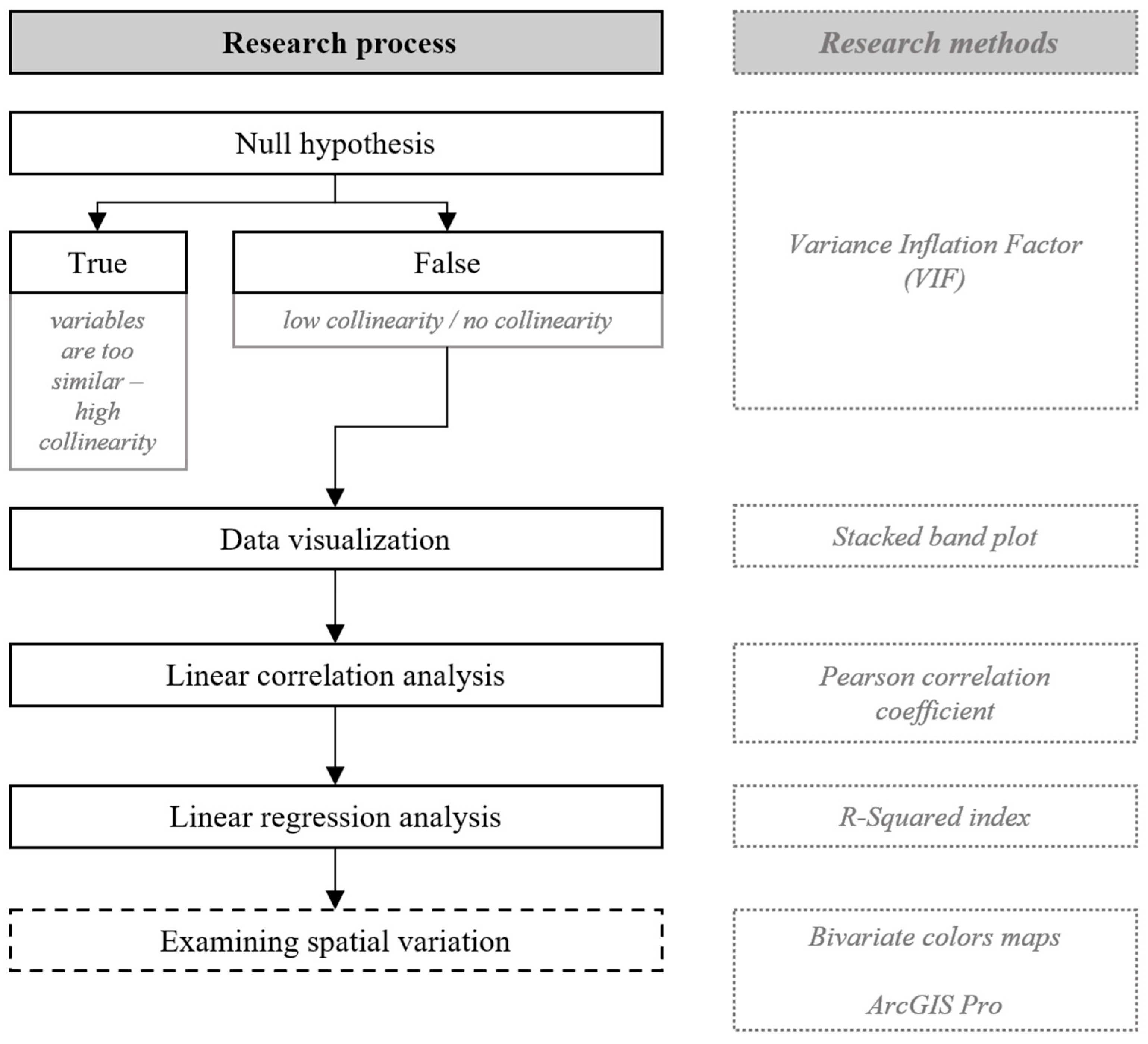
Before the main analysis began, the null hypothesis was established: the explanatory variables are highly similar and exhibit significant collinearity. To test this assumption, the Variance Inflation Factor (VIF) analysis was conducted as the first step of the data-processing stage. The absence of collinearity is a fundamental assumption of regression analysis.

The test was performed for each year of analysis separately, while results above VIF = 5 for any year declassified the model and did not allow for the rejection of the null hypothesis. Therefore, the VIF values for the first consecutive year of analysis, where VIF > 5, are included in the text. The test results for 2005 are included in

Table 3. Results of the first VIF test, year 2005. Source: own elaboration.

Working Variable Symbol	VIF
T1	1639.8
T2	2012.6
T3	342.4
T4	819.9
T5	2087.8
T6	769.9
T7	2.8
T8	12.9
T9	130.4
T10	122.4
T11	570.5
T12	36.1
T13	33.7
T14	5.7
T15	5.6
T16	5.6

below.

The analysis revealed a high degree of collinearity among many explanatory variables over multiple years. In order to improve the quality of the model and reject the null hypothesis test, it was decided to reject certain variables. An additional correlation analysis, using a Pearson correlation matrix, was conducted to identify variables most likely responsible for the excessive collinearity. The correlation matrix is presented in

Table 4. Results of Pearson correlation analysis for the first stage of VIF, example year 2005. Source: own elaboration.

	T1	T2	T3	T4	T5	T6	T7	T8	T9	T10	T11	T12	T13	T14	T15
T2	0.85
T3	0.79	0.64
T4	0.85	0.91	0.48
T5	0.91	0.98	0.72	0.90
T6	0.78	0.60	0.95	0.45	0.68
T7	0.08	0.38	0.11	0.19	0.33	0.01
T8	0.49	0.51	0.67	0.44	0.54	0.53	0.09
T9	0.56	0.35	0.49	0.26	0.37	0.56	−0.08	0.06
T10	0.29	0.17	0.20	0.17	0.18	0.27	−0.18	−0.07	0.81
T11	0.82	0.60	0.90	0.47	0.67	0.97	0.03	0.42	0.70	0.37
T12	0.06	−0.11	−0.05	−0.15	−0.09	0.01	−0.27	−0.12	0.14	0.06	0.02
T13	0.03	0.01	0.11	−0.05	0.00	0.23	−0.31	0.05	0.47	0.70	0.22	−0.08
T14	0.47	0.57	0.41	0.46	0.55	0.26	0.32	0.35	0.34	0.11	0.34	−0.23	−0.17
T15	0.38	0.27	0.49	0.20	0.30	0.51	−0.24	0.67	0.33	0.14	0.50	−0.10	0.39	0.27
T16	−0.36	−0.45	−0.05	−0.38	−0.39	−0.17	−0.04	0.30	−0.42	−0.30	−0.29	−0.28	−0.07	−0.27	0.17

.

The multiple occurrences of the coefficient deviating from 0 gave a reason to remove the variable from the model. This occurred for 7 variables: T1, T3, T4, T5, T6, T9, and T11. After this step, nine explanatory variables remained, and their summary is shown in

Table 5. Remaining indicators describing the Environmental Dimension of Sustainable Development, the second stage of data processing. Source: own elaboration.

Variable Description			Unit	Working Variable Symbol
Pollutant loads in wastewater discharged to water or ground	gaseous	carbon dioxide (CO2)	t/year	T2
Number of days in the year, where the maximum daily eight-hour mean of ozone (O3) level exceeds 125 micrograms per cubic meter (µg/m3)			Number of days	T7
Annual average concentration of particulate matter less than or equal to 10 microns in size (PM10)			µg/m3	T8
Pollutant loads in wastewater discharged to water or ground	chemical oxygen demand (COD)		kg/year	T10
	total nitrogen (N)		kg/year	T12
	total phosphorus (P)		kg/year	T13
Expenditure on environmental protection fixed assets per capita			PLN	T14
Share of green areas in the total area			%	T15
Share of legally protected areas in the total area			%	T16

.

The data prepared in this way formed the basis for the second round of the VIF test. The results of the test are shown in

Table 6. Results of the first VIF test, year 2009. Source: own elaboration.

Working Variable Symbol	VIF
T2	4.2
T7	23.2
T8	4.4
T10	5.7
T12	5.2
T13	22.4
T14	2.7
T15	2.7
T16	9.1

.

The second performed VIF test showed small excesses of the index, only in a few years of analysis. This indicated that the model was close to achieving the non-collinearity of the variables. Again, an additional correlation analysis of the variables was performed using the Pearson correlation matrix, the results of which are presented in

Table 7. Results of Pearson correlation analysis for the first stage of VIF, example year 2009. Source: own elaboration.

	T2	T7	T8	T10	T12	T13	T14	T15
T7	0.51
T8	0.48	0.20
T10	0.08	0.03	−0.12
T12	−0.14	−0.09	0.01	0.37
T13	0.47	0.78	0.17	0.52	0.18
T14	0.67	0.48	0.28	0.25	−0.26	0.56
T15	0.20	0.24	0.59	0.01	−0.10	0.35	0.23
T16	−0.41	−0.65	0.08	−0.32	−0.37	−0.54	−0.29	0.08

.

The second stage of the VIF resulted in the removal of three variables from the model: T14, T15, and T16; as a result, six explanatory variables were left in the model. A summary of these variables is included in

Table 8. Remaining indicators describing the Environmental Dimension of Sustainable Development, the third stage of data processing. Source: own elaboration.

Variable Description			Unit	Working Variable Symbol	Variable Symbol
Pollutant loads in wastewater discharged to water or ground	gaseous	carbon dioxide (CO2)	t/year	T2	V1
Number of days in the year, where the maximum daily eight-hour mean of ozone (O3) level exceeds 125 micrograms per cubic meter (µg/m3)			Number of days	T7	V2
Annual average concentration of particulate matter less than or equal to 10 microns in size (PM10)			µg/m3	T8	V3
Pollutant loads in wastewater discharged to water or ground	chemical oxygen demand (COD)		kg/year	T10	V4
	total nitrogen (N)		kg/year	T12	V5
	total phosphorus (P)		kg/year	T13	V6

.

The third VIF test was performed for the six variables in the table above, and its results for all years of analysis are shown in

Table 9. Results of the final VIF test. Source: own elaboration.

Variable Symbol	VIF
	2005	2006	2007	2008	2009	2010	2011	2012	2013	2014	2015	2016	2017	2018	2019	2020	2021	2022	2023
V1	1.88	1.69	1.51	1.78	1.81	3.36	1.98	0.60	2.66	3.47	2.61	3.22	2.31	2.32	2.13	1.79	2.01	2.54	4.28
V2	1.48	1.38	1.27	1.18	4.09	2.38	1.26	0.44	2.15	1.67	1.72	1.83	3.46	1.30	1.26	1.02	1.54	1.22	2.03
V3	1.55	1.63	1.37	1.27	1.40	1.80	1.91	0.49	2.28	2.88	2.83	3.40	4.28	2.46	1.93	1.75	2.00	2.60	2.93
V4	2.40	3.18	1.91	1.56	2.80	2.66	2.36	0.49	1.75	1.82	1.68	1.66	2.26	3.25	3.39	1.50	2.93	1.28	4.00
V5	1.16	1.64	1.09	1.22	1.29	1.26	1.25	0.16	1.20	1.24	1.25	1.26	1.26	1.16	1.16	1.12	1.11	1.08	1.09
V6	2.37	3.10	1.95	1.96	4.03	2.04	2.30	0.58	2.08	1.87	1.90	2.05	2.26	3.35	3.67	1.55	2.58	1.35	2.92

.

The results of the third VIF test confirmed the achievement of optimal model parameters, thus allowing for the rejection of the null hypothesis. Finally, for the description of the Environmental Dimension of Sustainable Development, the following variables were selected (these variables are commonly used in studies on describing the state of the natural environment):

• V1—carbon dioxide (CO₂) emissions from facilities especially noxious to air purity [74,75,76,77].
• V2—number of days in the year, where the maximum daily eight-hour mean of ozone (O₃) level exceeds 125 micrograms per cubic meter (µg/m³) [78,79,80].
• V3—annual average concentration of particulate matter less than or equal to 10 microns in size (PM₁₀). PM10 means particulate matter that passes through a size-selective inlet as defined in the reference method for the sampling and measurement of PM₁₀, EN 12341 [81], with a 50% efficiency cut-off at 10 µm aerodynamic diameter [74,82,83].
• V4—the chemical oxygen demand (COD) pollutant loads in wastewater discharged to water or ground. COD is an indicative measure of the amount of oxygen that can be consumed by reactions in a measured solution. The most common application of COD is in quantifying the amount of oxidizable pollutants found in surface water (e.g., lakes and rivers) or wastewater [84,85,86].
• V5—pollution loads of total nitrogen (N) in wastewater discharged to water or the ground [87,88,89].
• V6—pollution loads of total phosphorus (P) in wastewater discharged to water or the ground [90,91,92].

Thus prepared, the database formed the basis for examining the relations between the Environmental Dimension of Sustainable Development and the transition from brown to green energy.

3.2. Environmental Dimension of Sustainable Development in Relation to the Transition from a Brown to a Green Energy

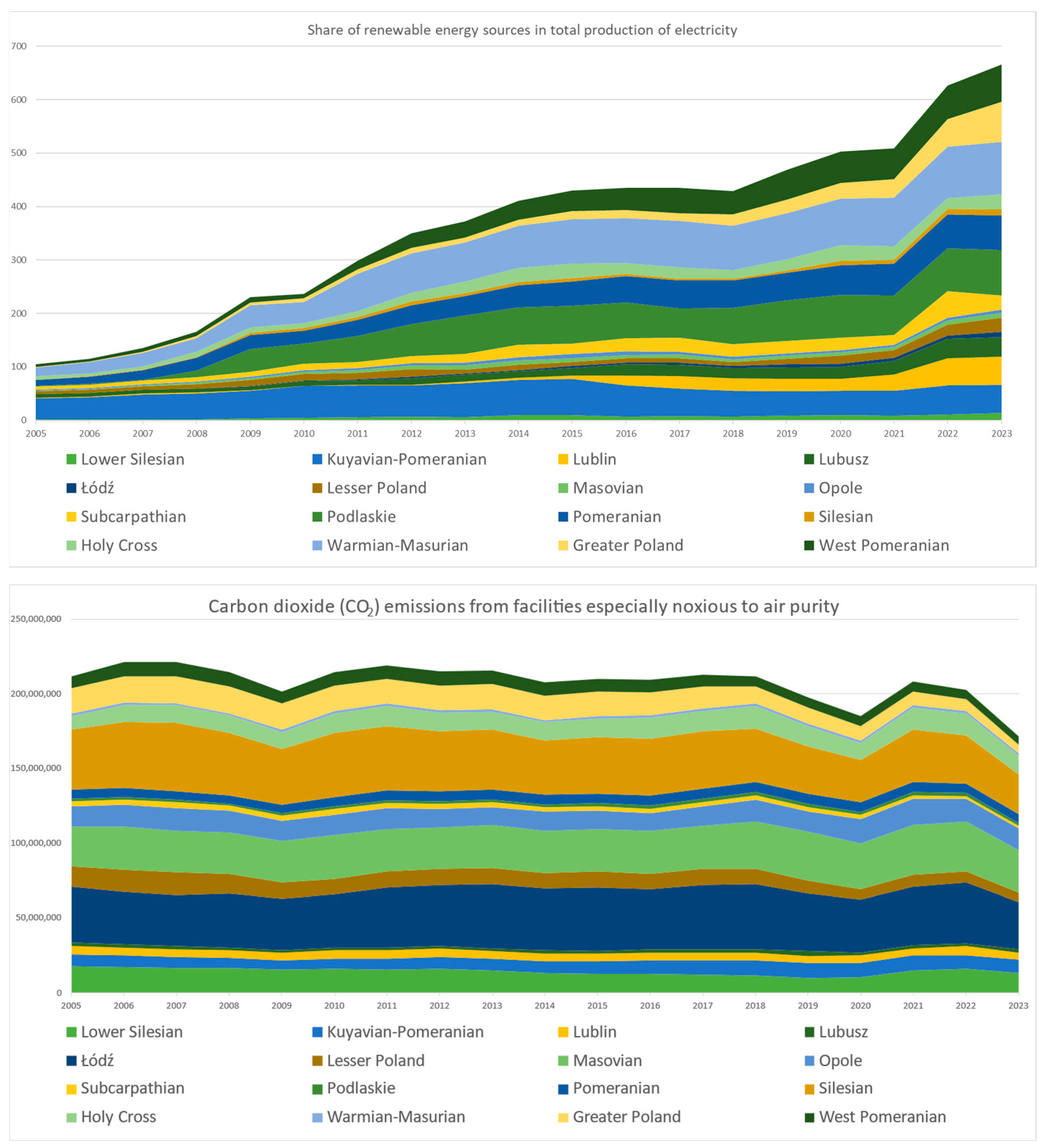
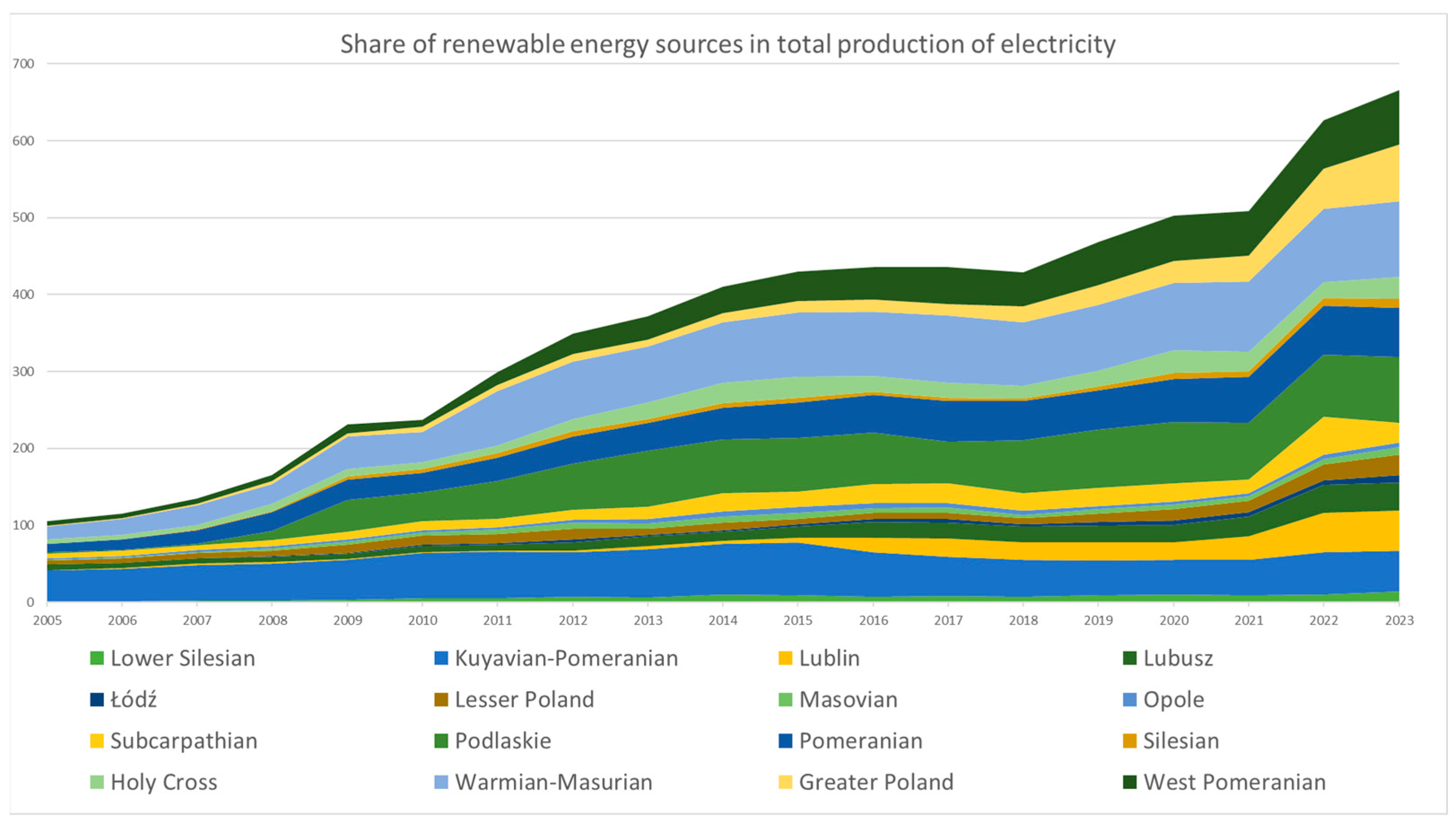
The first step in analyzing the process of transition from brown energy to green energy in Poland’s voivodeships involved visualizing the data using cumulative layer charts, which are commonly used to illustrate changes in phenomena over time. Even this basic visualization method allows for the formulation of initial conclusions, which will then be refined in subsequent stages of this study. Figure 3 presents a graph of changes in the share of renewable energy in total electricity production.

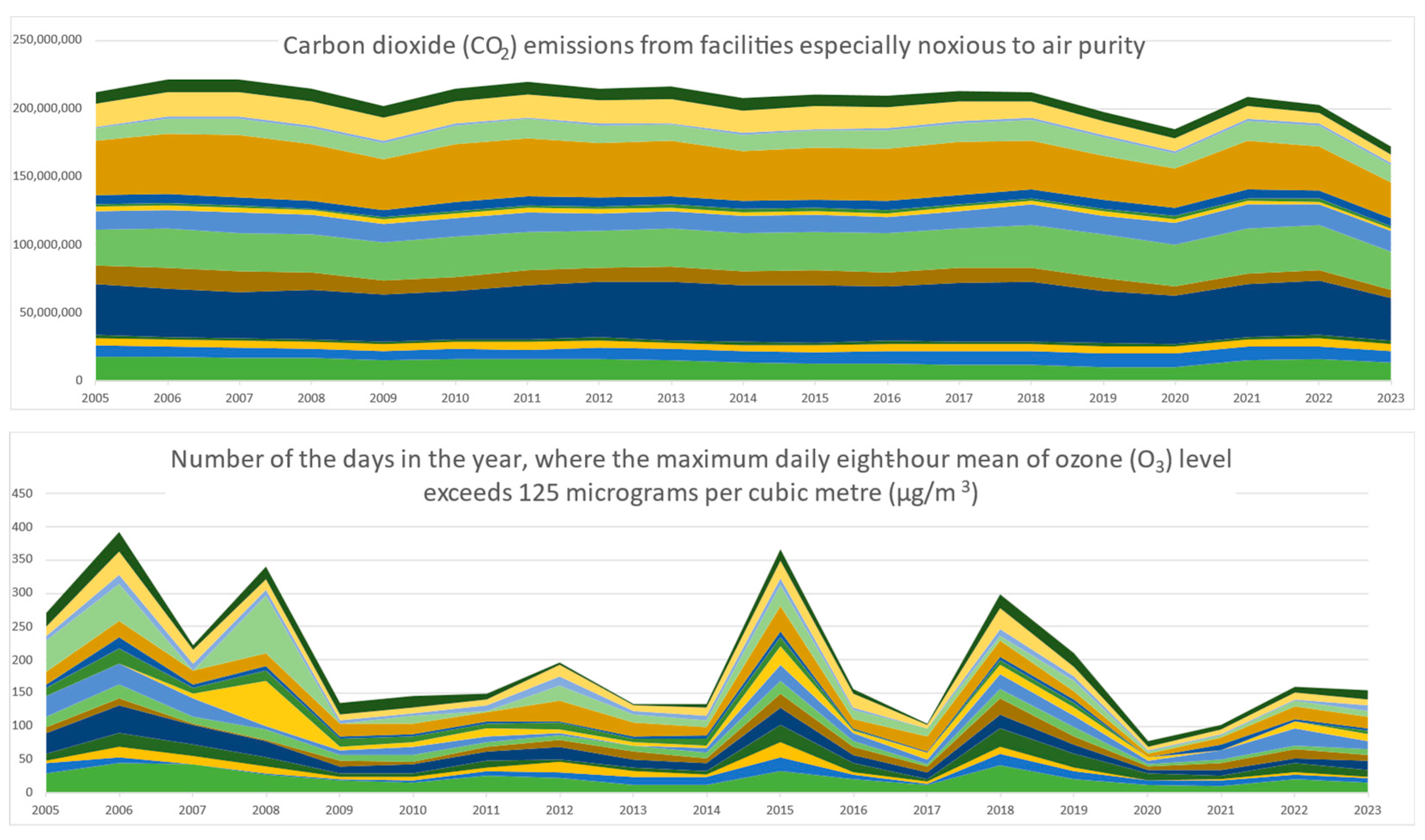
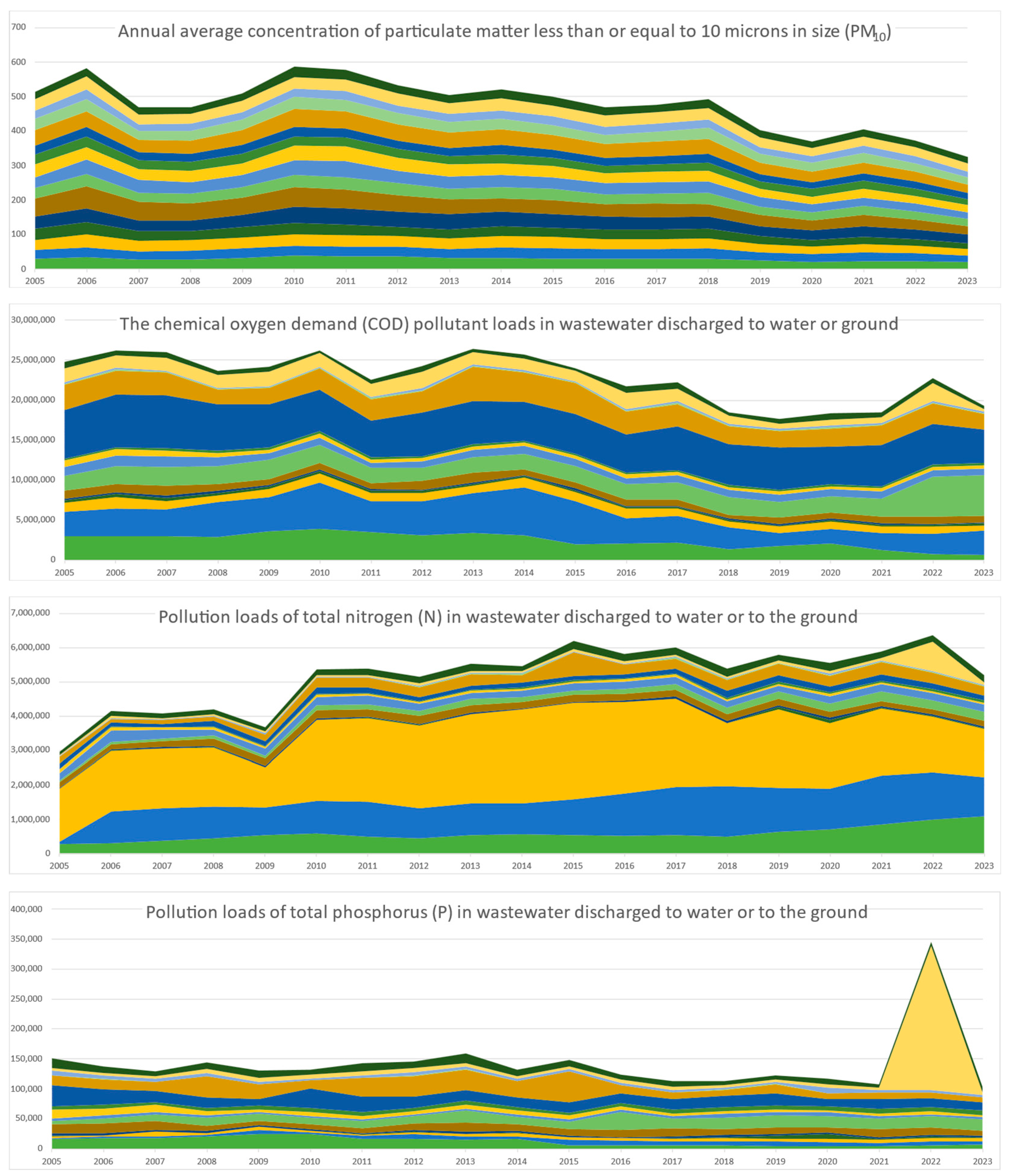
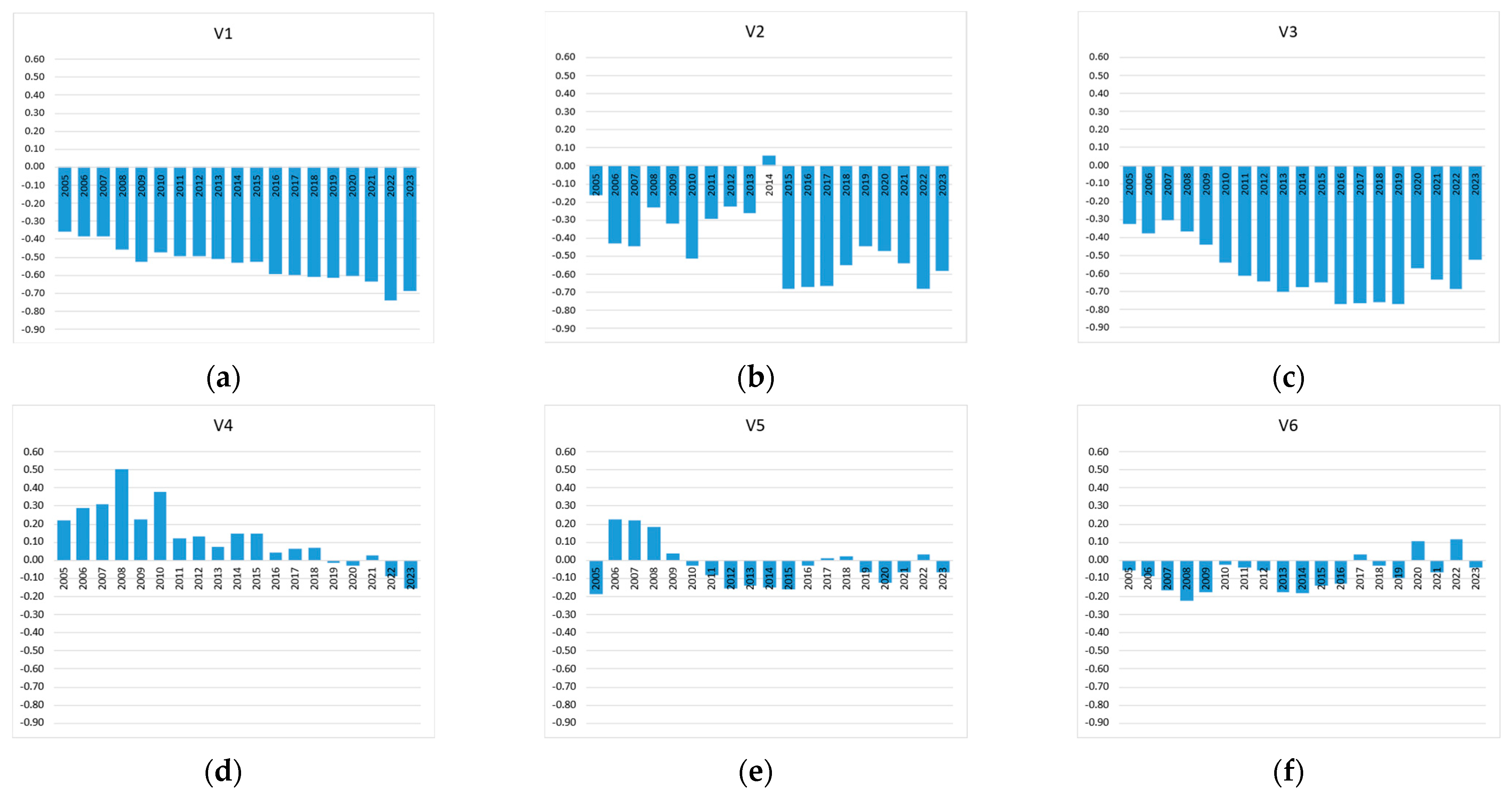
Despite the name of this method, the above graph cannot be interpreted cumulatively—it presents percentage data after all. Instead, it depicts the successive increase in the use of renewable energy sources across the country. The explanatory variables of the model were then visualized in a similar manner, and the results are presented in Figure 4.

To enhance the readability of the charts, simplified versions are included here. The full versions can be found at the end of the article, in the Appendix A. The above graphs show a general decrease in the level of environmental pollution, represented by the six selected indicators. The exception is the graph of variable V5, where an overall increase can be seen.

3.3. Testing Using Pearson’s Linear Correlation

The next step of the study was an analysis using Pearson’s linear correlation coefficient. Such a test allows for finding potential evidence of co-occurrence in the data. The tabular results are presented in

Table 10. Pearson’s correlation coefficient values for explanatory variables in 2005–2023.

Variable Symbol	Pearson’s Linear Correlation Coefficient
	2005	2006	2007	2008	2009	2010	2011	2012	2013	2014	2015	2016	2017	2018	2019	2020	2021	2022	2023
V1	−0.36	−0.38	−0.38	−0.46	−0.52	−0.47	−0.49	−0.49	−0.51	−0.53	−0.52	−0.59	−0.60	−0.61	−0.61	−0.60	−0.63	−0.74	−0.69
V2	−0.16	−0.43	−0.45	−0.23	−0.32	−0.51	−0.29	−0.22	−0.26	0.06	−0.68	−0.67	−0.67	−0.55	−0.45	−0.47	−0.54	−0.68	−0.58
V3	−0.33	−0.37	−0.30	−0.36	−0.44	−0.54	−0.61	−0.64	−0.70	−0.68	−0.65	−0.77	−0.76	−0.76	−0.77	−0.57	−0.63	−0.69	−0.52
V4	0.22	0.29	0.31	0.50	0.23	0.38	0.12	0.13	0.07	0.15	0.15	0.04	0.06	0.07	−0.01	−0.03	0.03	−0.09	−0.15
V5	−0.19	0.23	0.22	0.18	0.04	−0.03	−0.08	−0.15	−0.14	−0.15	−0.16	−0.03	0.01	0.02	−0.07	−0.13	−0.07	0.03	−0.07
V6	−0.06	−0.09	−0.16	−0.22	−0.17	−0.03	−0.04	−0.05	−0.18	−0.18	−0.14	−0.13	0.03	−0.03	−0.10	0.11	−0.07	0.12	−0.04

.

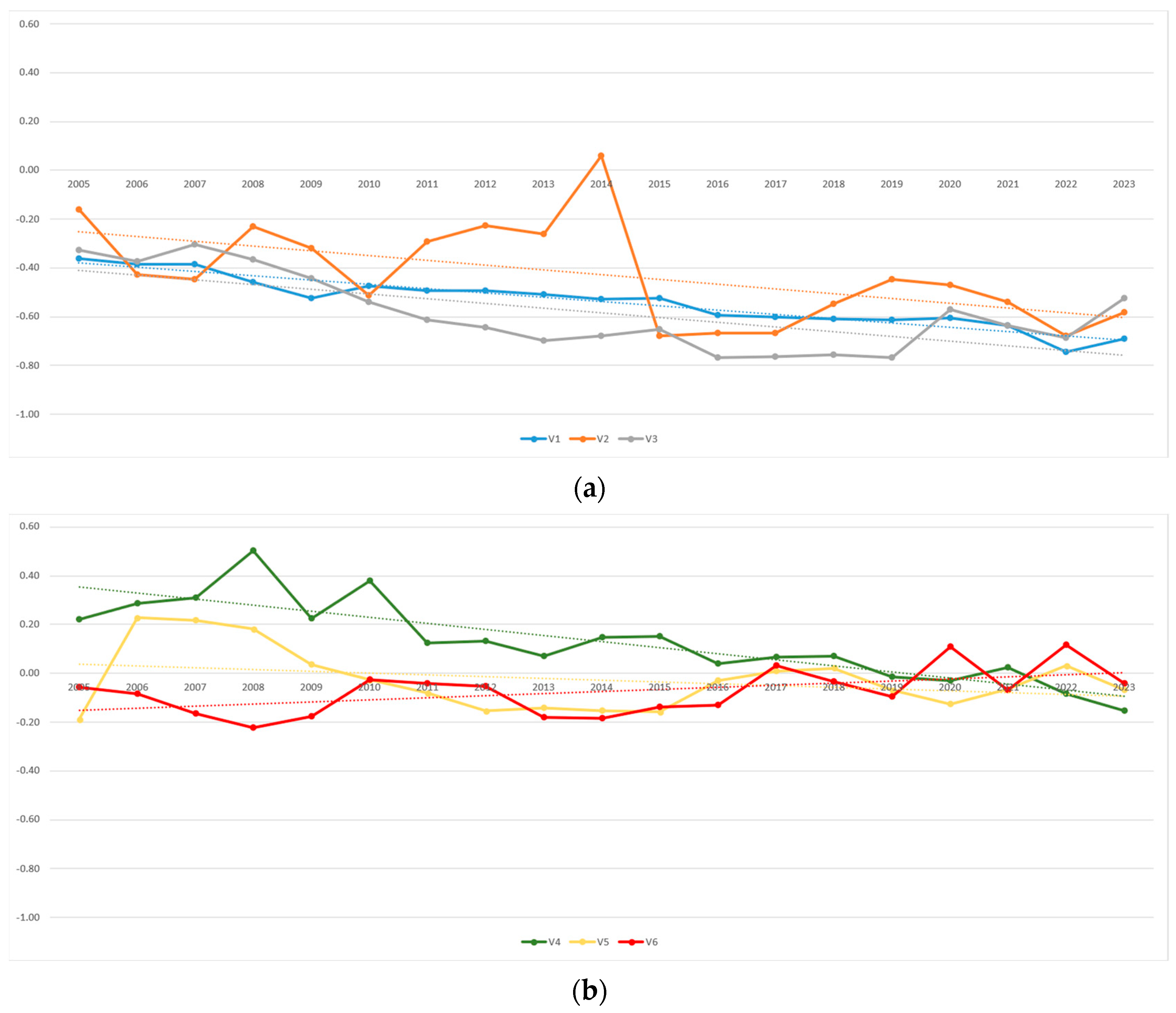
For all analyzed variables, the coefficient values fall in the range <−0.77; 0.50>. Of the 114 values (6 variables, 19 years), as many as 88 are negative—this indicates a general trend of inverse (or negative) correlation. Most of the coefficients indicate weak correlation (62 in total), but this is mainly observed for variables V4–V6, i.e., describing pollution of water and ground (56 coefficients). Moderate correlation is indicated by 47 coefficients, almost all for variables describing air pollution (46 coefficients, for variables V1–V3). The remaining 5 coefficients indicate a strong correlation (4 for variable V3, 1 for variable V1). The results suggest a weak correlation of water and ground pollution, while a negative moderate and negative strong correlation for the air pollution variables. In order to better illustrate the results, the data are presented in the column graphs below (Figure 5). The axes of the charts have been unified to allow comparison of the results.

The column graphs illustrate changes in values over time. Pearson’s correlation coefficient values for most variables are gradually decreasing. Changes for variables V1–V3 are lower and more stabilized—values are successively decreasing. For variables V4–V6, the situation is more dynamic, with values increasing and decreasing by different ranges. In order to look for trends in the changes in the studied phenomenon, it was decided to combine the data thematically into variables describing air pollution (V1–V3) and variables describing water and ground pollution (V4–V6) in two separate line graphs, which are presented in Figure 6.

By presenting the data in this way, the downward trend of the correlation coefficient is clearly visible. The addition of a linear trend line further emphasizes this relationship. The line is downward for most variables, except for variable V6.

3.4. Testing Using Linear Regression

The final stage of the study was to perform a linear regression analysis. However, before calculating the model fit measure, it was necessary to verify the robustness of the regression input data. The variables were analyzed using the p-value index, testing the statistical significance of the data. The results of the analysis are presented in

Table 11. Results of p-value test. Source: own elaboration.

Variable Description			Unit	Variable Symbol	p-Value
Pollutant loads in wastewater discharged to water or ground	gaseous	carbon dioxide (CO2)	t/year	V1 **	0.00
Number of days in the year, where the maximum daily eight-hour mean of ozone (O3) level exceeds 125 micrograms per cubic meter (µg/m3)			Number of days	V2 **	0.00
Annual average concentration of particulate matter less than or equal to 10 microns in size (PM10)			µg/m3	V3 **	0.00
Pollutant loads in wastewater discharged to water or ground	chemical oxygen demand (COD)		kg/year	V4 *	0.04
	total nitrogen (N)		kg/year	V5 *	0.02
	total phosphorus (P)		kg/year	V6 *	0.03

Note: **—statistically significant at the p < 0.01 level; *—statistically significant at the p < 0.05 level.

.

All variables are statistically significant, variables V1–V3 at the p < 0.01 level and variables V4–V6 at the p < 0.05 level. The R-Squared coefficient of determination was then used as a measure of the fit of the statistical model of the transition process from brown energy to green energy. The following

Table 12. R-Squared values for the entire model from 2005 to 2023. Source: own elaboration.

	2005	2006	2007	2008	2009	2010	2011	2012	2013	2014	2015	2016	2017	2018	2019	2020	2021	2022	2023
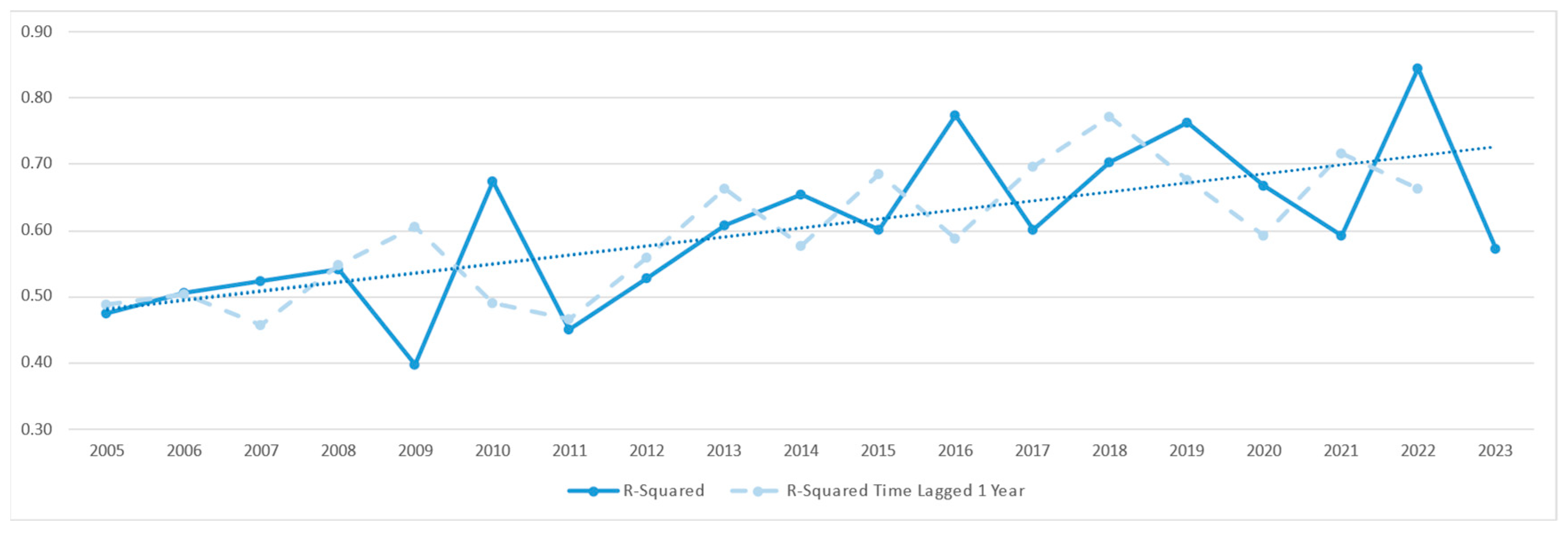
R-Squared	0.48	0.51	0.52	0.54	0.40	0.67	0.45	0.53	0.61	0.66	0.60	0.77	0.60	0.70	0.76	0.67	0.59	0.84	0.57

contains R-Squared values for the following assumptions: the dependent variable is the share of renewable energy in total electricity production, and the explanatory variables are V1–V6.

R-Squared values are within the range <0.40; 0.84>, indicating a good to very good model fit. The values for 15 of the 19 years of analysis (11 of which are 2005–2015, the first years of the study’s time range) are in the <0.4; 0.7) range, and the remaining 4 are in the <0.71; 0.84> range. This indicates an upward trend in the model fit measure; to analyze the results in more detail, the results are shown with a line graph below (Figure 7). In order to validate the near-immediate impact on the environment of the way energy is produced, a 1-year time lag was additionally included in the graph (the statistical model was slightly modified with the following assumptions: the dependent variable from a given year and the explanatory variables from the following year).

Despite the presence of deviations, the linear trend line is an upward line. Introduced time lag did not significantly affect the result of the analysis (trend lines overlap). In order to examine the phenomenon more closely, it was decided to divide the model into two parts: the first, in which the explanatory variables were only those describing air pollution (variables V1–V3), and the second, in which the explanatory variables were only those describing water and ground pollution (variables V4–V6). The results are presented in

Table 13. R-Squared values for model V1–V3 and model V4–V6, from 2005 to 2023. Source: own elaboration.

	R-Squared
	2005	2006	2007	2008	2009	2010	2011	2012	2013	2014	2015	2016	2017	2018	2019	2020	2021	2022	2023
V1–V3 variables	0.16	0.34	0.30	0.31	0.33	0.41	0.40	0.44	0.53	0.61	0.55	0.66	0.60	0.67	0.70	0.62	0.54	0.83	0.53
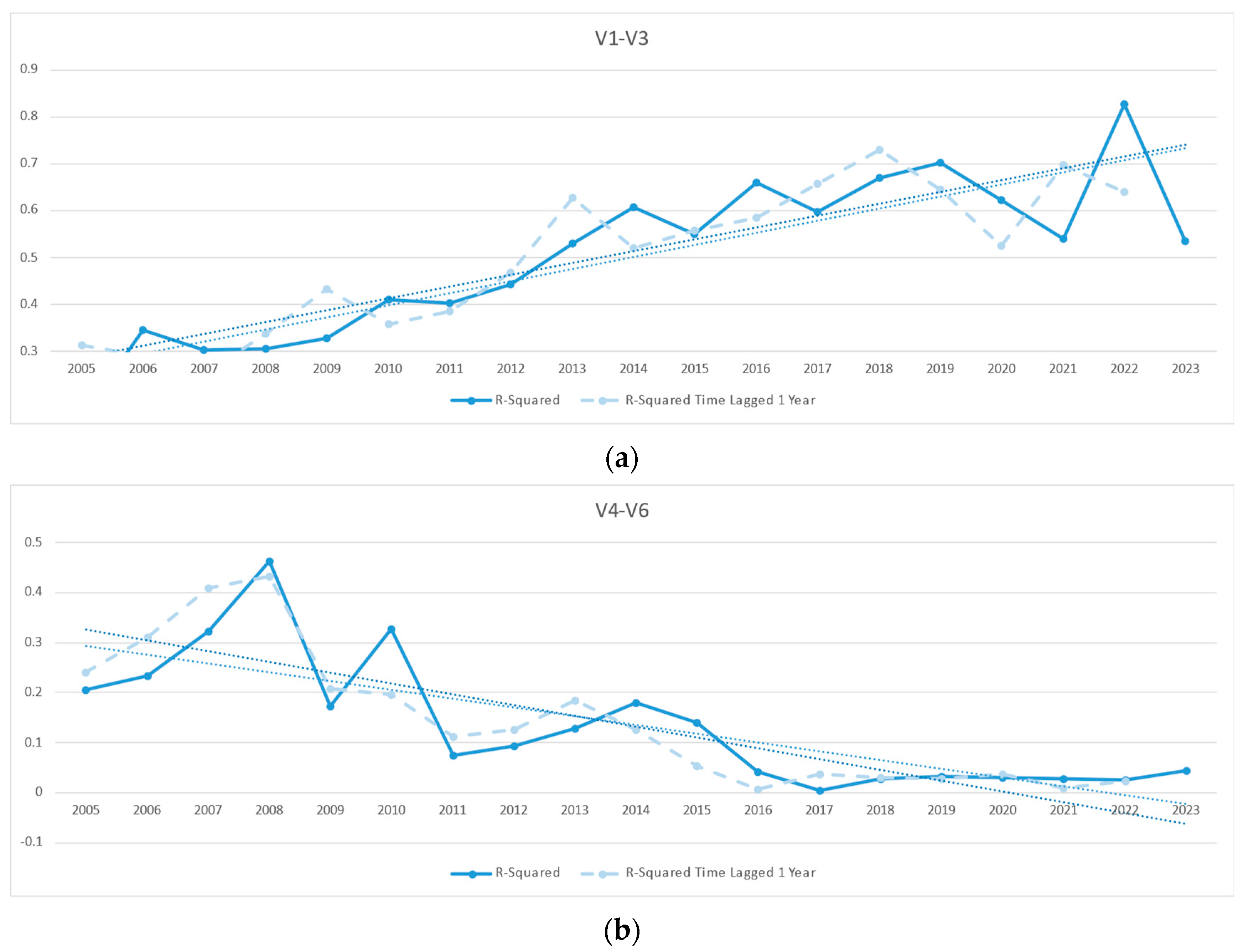
V4–V6 variables	0.20	0.23	0.32	0.46	0.17	0.33	0.08	0.09	0.13	0.18	0.14	0.04	0.00	0.03	0.03	0.03	0.03	0.03	0.05

below.

When broken down into two types of environmental pollution, a large discrepancy between the results can be seen. In the case of the model for V1–V3 variables, the R-Squared value is in the range <0.159; 0.828>, while in the case of the model for V4–V6 variables, it is in the range <0.004; 0.463>. The difference in these ranges is very high: in the V4–V6 model, 18 of the 19 indicators are values below 0.4 (in comparison, the V1–V3 model has five such values), and in the V1–V3 model, 14 of the 19 indicators are values above 0.4 (of these, two are values above 0.7), while there is only one indicator in such a range in the V4–V6 model. R-Squared values for the V1–V3 and V4–V6 models are presented in Figure 8.

The differences between the model fit measures of air pollution (model V1–V3) and water and ground pollution (model V4–V6) are very noticeable. The linear trend line of the first model takes on a positive value, while that of the second model takes on a negative value. As in Figure 7, the introduced time lag does not significantly affect the results.

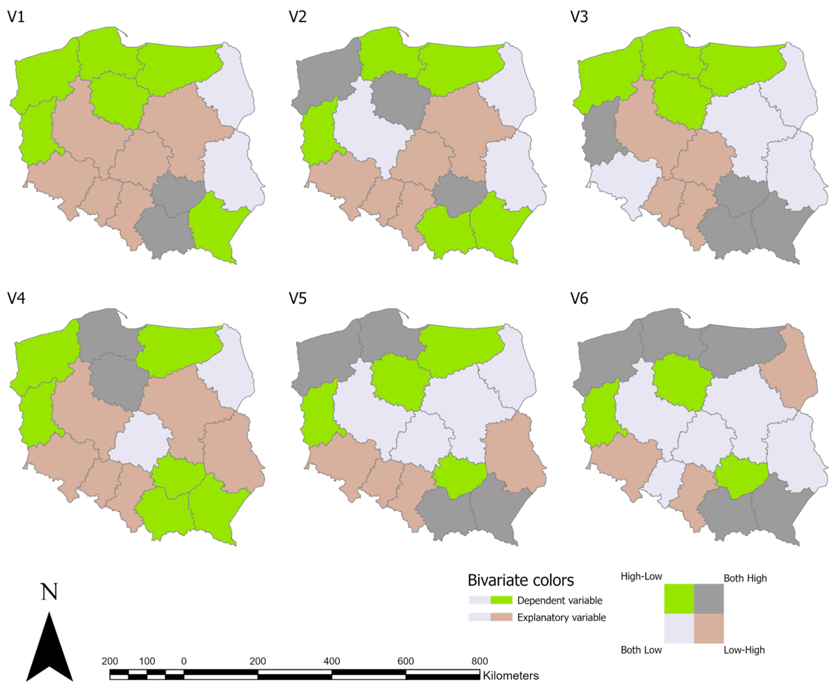
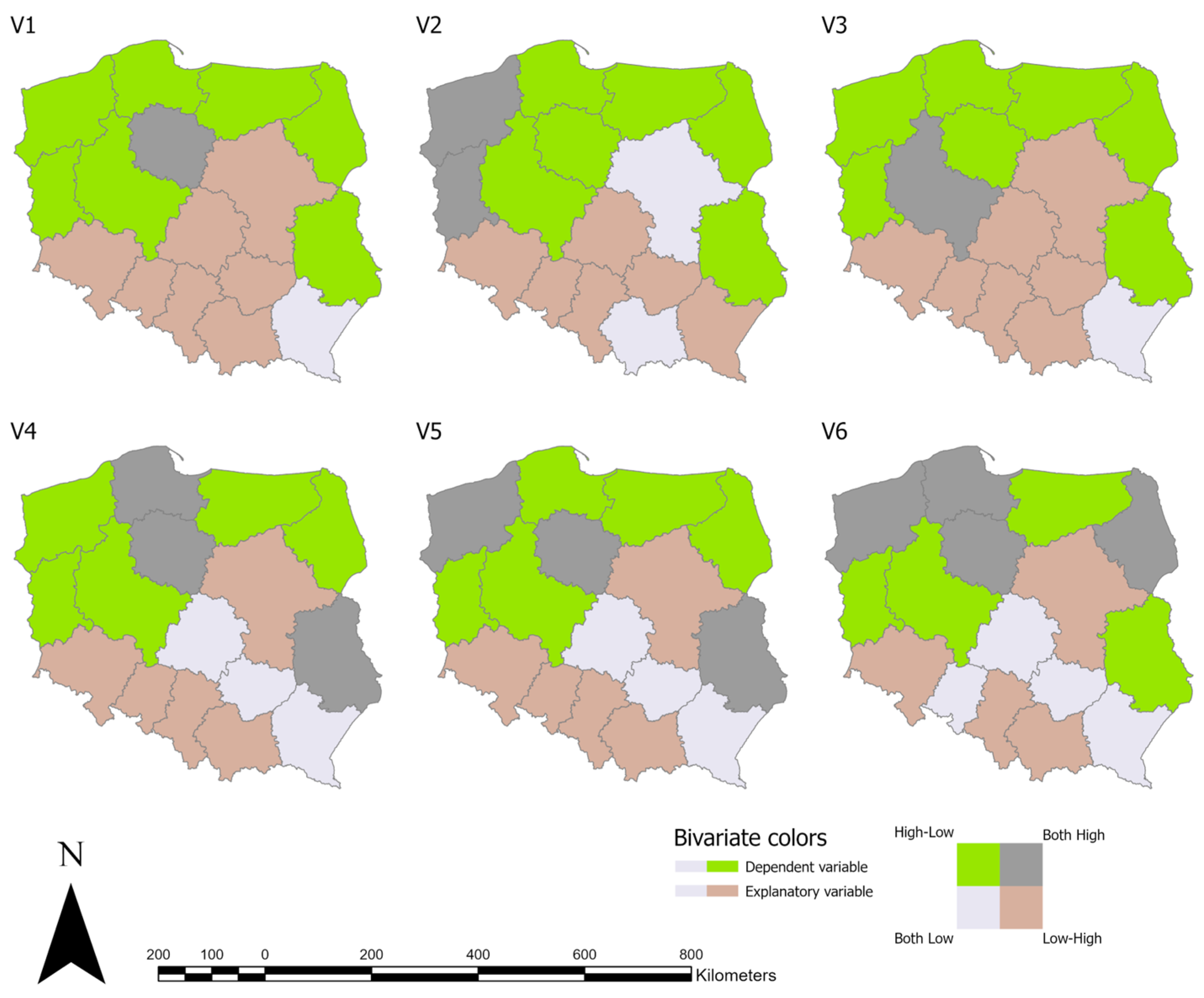
3.5. Testing Local Variations Using the Bivariate Colors Method

The final component of the study was the analysis of local variations using GIS tools in ArcGIS Pro 3.4. A particular type of choropleth map, the bivariate colors method, was used to visualize the quantitative relationship between two variables. In this way, six maps were prepared to visually compare the co-occurrence of the dependent variable and the six individual explanatory variables. The results for 2005 are presented in Figure 9.

In order to illustrate the changes in the relationship of the aforementioned variables in Poland’s voivodeships over the entire time range of the analysis, data for 2023 (Figure 10) were similarly visualized.

These maps illustrate the spatial distribution of the relationship between the dependent variable and the explanatory variables in 2005 and 2023.

The high–low class—indicating a high share of renewable energy sources in total electricity production and low levels of environmental pollution—is marked in green. This class indicates the most favorable relationship between the analyzed variables, from the perspective of the research conducted in the article.

The low–high class, marked in brown, indicates a low share of renewable energy sources in total electricity production and high levels of environmental pollution. This represents the most unfavorable relationship between the variables under analysis.

The other two classes, high–high (marked in dark gray) and low–low (marked in light gray), indicate, respectively, high share of renewable energy sources in total electricity production and high levels of pollution; and low share of renewable energy sources in total electricity production and low levels of pollution. These patterns neither confirm nor contradict the expected trends and, therefore, do not directly support a positive relationship between the variables, in the context of the study’s objectives.

The following

Table 14. Number of voivodeships per class, in 2005. Source: own elaboration.

	High–Low	Low–High	High–High	Low–Low
V1	6	6	2	2
V2	5	5	3	3
V3	4	4	4	4
V4	6	6	2	2
V5	4	4	4	4
V6	3	3	5	5
Overall	28	28	20	20

and

Table 15. Number of voivodeships per class, in 2023. Source: own elaboration.

	High–Low	Low–High	High–High	Low–Low
V1	7	7	1	1
V2	6	6	2	2
V3	7	7	1	1
V4	5	5	3	3
V5	5	5	3	3
V6	4	4	4	4
Overall	34	34	14	14

present the results of the study using the bivariate colors method.

When comparing the results for the two extreme years of the time range of the analysis, there is a clear increase in the marginal high–low and low–high classes (in both cases an increase of 6 voivodeships). Large changes can be seen especially for variable V3 (annual average concentration of particulate matter PM₁₀), where class changes were recorded in three voivodeships.

A detailed comparative analysis of the two states presented in the maps for 2005 and 2023 allows for additional conclusions to be drawn regarding drastic changes in the relationships between the variables under study. These include two situations—the first, when a voivodeship changes class from low–high to high–low, and the reverse, when a voivodeship changes class from high–low to low–high. From the point of view of the research conducted in the article, the first situation is a positive one, and it was recorded in two cases—in the Greater Poland Voivodeship, for variables V1 and V4. The second situation, which is negative from the point of view of the research conducted in the article, occurred for two voivodeships—Subcarpathian for variable V2 and Lesser Poland for variable V4.

4. Discussion and Conclusions

The primary objective of this study was to comprehensively trace the transition from brown energy to green energy, in relation to the Environmental Dimension of Sustainable Development. During the initial stages of statistical analysis, the number of explanatory variables was significantly reduced—out of the initially selected 16 variables, only 6 were eventually used to build the model. This was due to the excessive multicollinearity of the variables, which was confirmed by all stages of the VIF indicator study. In the authors’ view, this substantial reduction did not compromise the integrity of the study, as the retained variables continued to accurately reflect the state of the environment, which is one of the most important elements of the Environmental Dimension of Sustainable Development [55].

To measure the shift from brown to green energy across Polish voivodeships, the percentage share of renewable energy in total electricity production was selected as the dependent variable. According to the data presented in Figure 3, this share is gradually increasing nationwide, although the pace of change varies significantly between regions.

Aligned with global sustainability trends [93,94,95,96,97,98,99], the data confirm a national upward trend in the share of renewable energy. However, regional disparities are evident. Taking into account the selected time range of the analysis, most voivodeships at their beginning were characterized by a very low share of renewable energy in total electricity production—of the 16 voivodeships analyzed, for 13, this share was below 10% in 2005. By comparison, in 2023 (the last year of the analysis), only two voivodeships did not exceed this level (Masovian and Opole Voivodeships). The largest percentage increase was registered in Podlaskie Voivodeship, with an increase of 84.1 percentage points (from 1.3% to 85.4%), followed by Warmian-Masurian Voivodeship (80.8 percentage points, up from 16.8% to 97.6%), and Greater Poland Voivodeship (73.9 percentage points, up from 0.7% to 74.6%). The smallest growth is in the Opole Voivodeship, with an increase of 4.7 percentage points (up from 1.5% to 6.2%).

Moreover, it can be seen that the rate of change in the share of renewable energy in electricity production varies from one voivodeship to another. Analyzing the initial and final year of the time range of the study, several different trends can be identified. Some voivodeships, compared to others, were already initially characterized by a high share of renewable energy. Despite this, the final year of the analysis registered an equally high share compared to other voivodeships. Such cases include, for example, the Warmian-Masurian Voivodeship (up from 16.8% to 97.6%) or the Pomeranian Voivodeship (up from 10.7% to 64.5%). Another trend is when a voivodeship has a low share of renewable energy in electricity production in the first year of analysis but a relatively very high share in the final year. Such a case is the aforementioned Podlaskie Voivodeship (up from 1.3% to 85.4%), as well as the Greater Poland Voivodeship (up from 0.7% to 74.6%), or Lublin Voivodeship (up from 0.4% to 52.9%). An exceptional case is the Kuyavian-Pomeranian Voivodeship, which initially had by far the highest share of renewable energy (40.1%). In subsequent years of analysis, this share fluctuated unevenly to reach 53% in the last year of analysis, which is not the highest value over the entire analysis period (in 2015, it was 68.6%).

These variations underscore the importance of using normalized measures (i.e., percentage shares) rather than absolute figures (e.g., GWh) to assess progress over time.

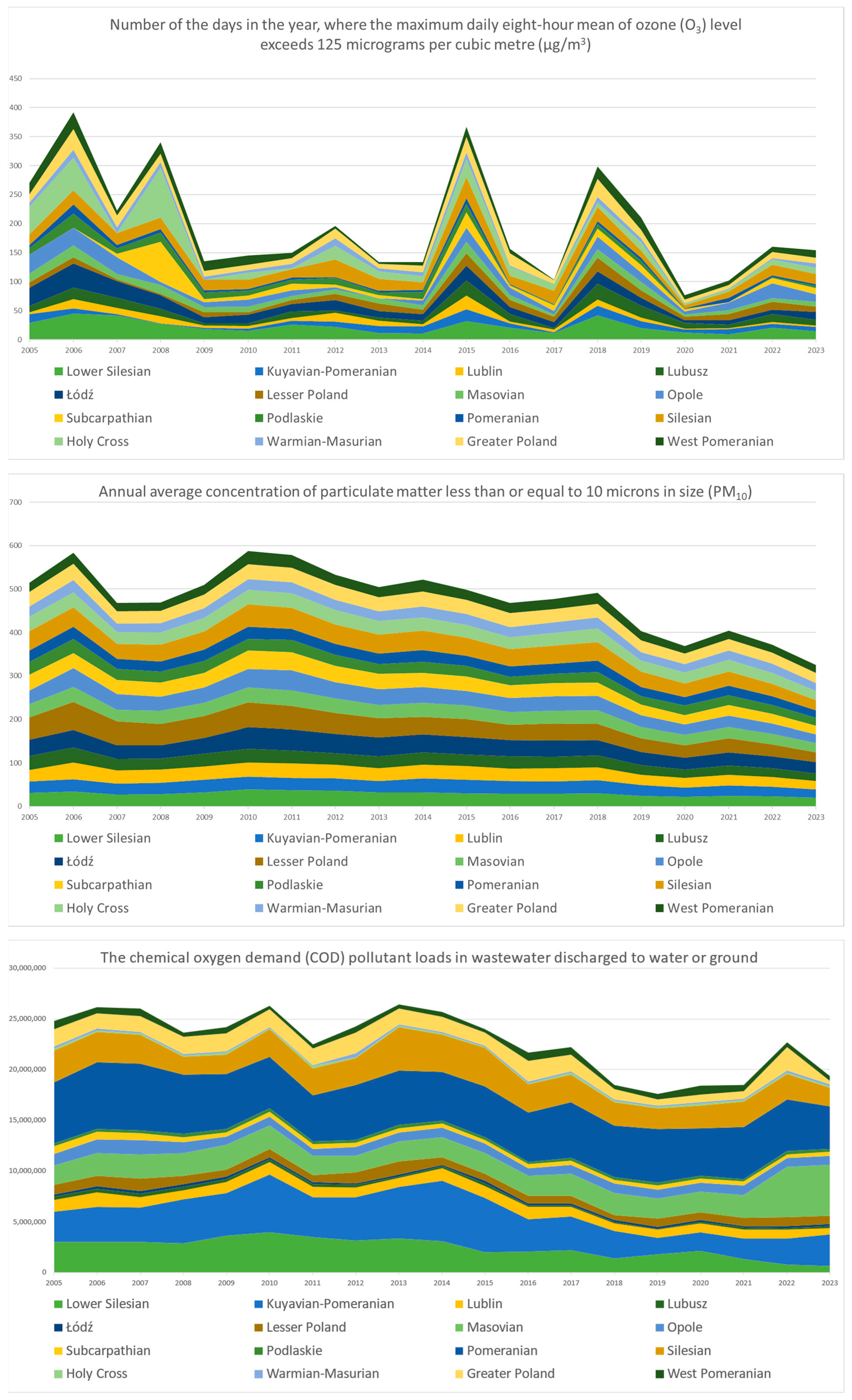
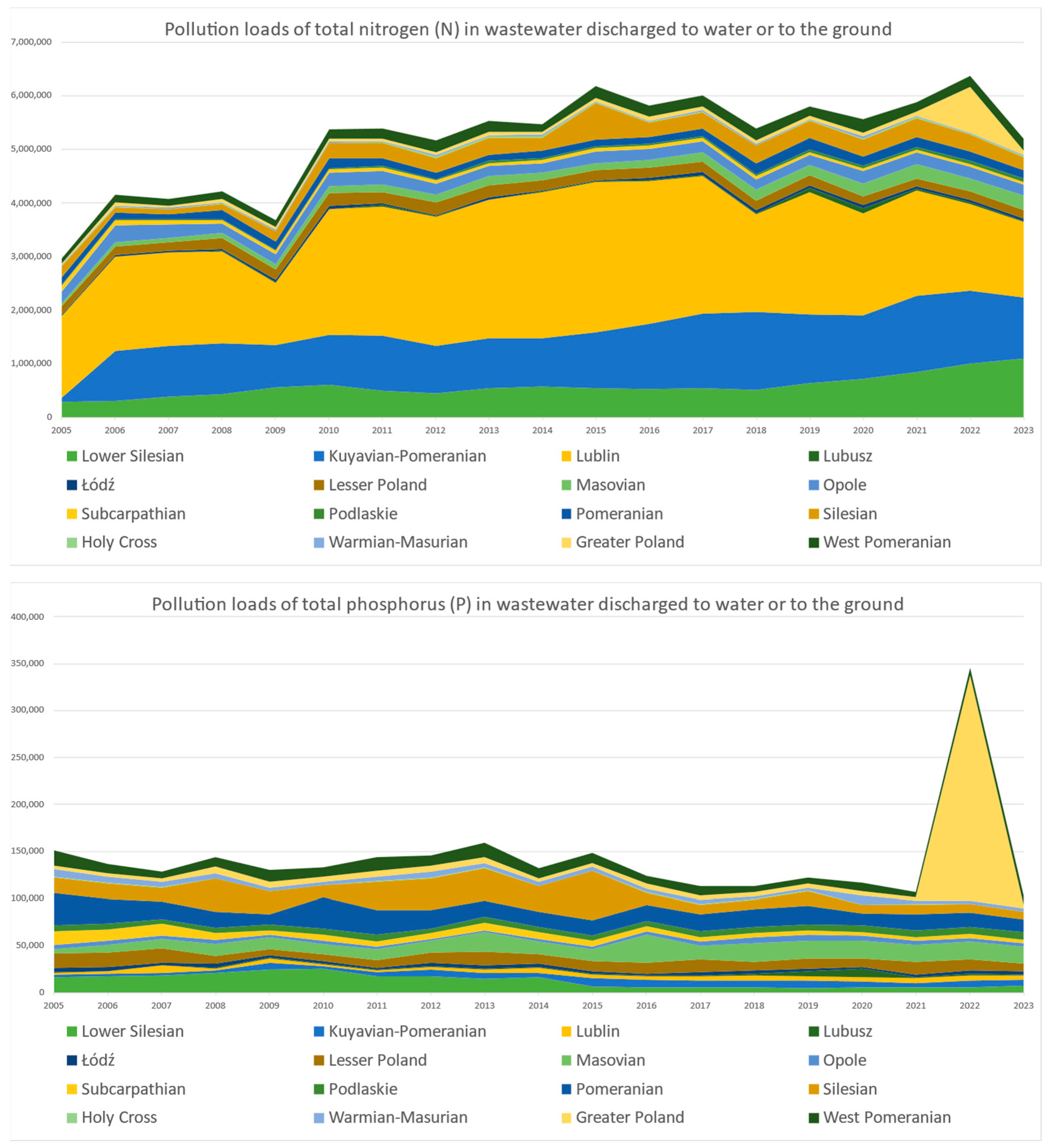
The visualization of the model’s explanatory variables (shown in Figure 4) reveals time-based trends. Variables describing air pollution are characterized by a successive decrease; although, in the case of ozone, this variability is subject to large fluctuations (Figure 5b). On the other hand, in the case of variables describing water and ground pollution, a downward trend was registered for only two variables (the chemical oxygen demand and total phosphorus load, Figure 5d,f, respectively). The graph of changes in total nitrogen load looks different: its level in the analyzed time range is increasing.

Analyzing the explanatory variables of the model on a voivodeship-by-voivodeship basis, there is one clear deviation from the overall trends. This situation applies to the Greater Poland Voivodeship in 2022, when there was a very noticeable increase in the level of variables describing water and ground pollution (Figure 5d–f), especially in the case of total phosphorus (Figure 5f).

Analysis using Pearson’s linear correlation coefficient made it possible to examine the co-occurrence of the dependent variable and the explanatory variables. The analysis found large differences in the correlation coefficient values between explanatory variables describing the state of air pollution (variables V1–V3) and describing the state of water and ground pollution (variables V4–V6). The results of the study in the Section 3 are therefore visualized in two separate graphs (Figure 6a,b). The vast majority of Pearson correlation coefficients take on negative values, indicating an inverse correlation. This may indicate that as the share of renewable energy in total electricity production increases, the level of environmental pollution in Poland’s voivodeships decreases. In the case of variables describing the state of air pollution (variables V1–V3), the correlation coefficient indicates a moderate correlation and a strong correlation in several cases. Thus, it cannot be said unequivocally that this relationship is very strong, but it confirms the general trend indicated earlier. Pearson’s correlation coefficient values for variables describing the state of water and ground pollution (variables V4–V6), on the other hand, indicate a weak correlation, close to zero. In this case, co-occurrence cannot be unequivocally confirmed.

Analyzing the distribution of variables for successive years of analysis, the graph for variables V1–V3 (Figure 6a) shows a relatively stable decrease in the value of Pearson’s correlation coefficient for variables V1 and V3 (describing, respectively, carbon dioxide emissions and annual average concentration of particulate matter PM₁₀). In the case of variable V2 (the number of days in the year, where the maximum daily eight-hour mean of ozone level exceeds 125 micrograms per cubic meter), the decrease is more chaotic, with many fluctuations. In the case of all three variables, a worrying change in the trend can be seen in the last year of analysis—all values of the correlation coefficient are increasing. This may indicate a future reversal of the trend and could be the basis for further follow-up studies in the future.

The regression analysis of the measure of fit of the statistical model clearly shows an increase in the fit of the explanatory variables to the dependent variable over time, confirming the conclusions of the Pearson’s correlation test. The measure of the fit of the statistical model involving all 6 explanatory variables, visualized in Figure 7, shows an increasing trend, with significant fluctuations evident. R-Squared values for this model indicate good to very good fit. After separating the model into two parts, describing independently the state of air pollution and the state of water and ground pollution, the obtained model fit results are very different. In the case of variables V1–V3, an upward trend in R-Squared values can be confirmed, in contrast to variables V4–V6, where this trend is downward (and R-Squared values in the last few years of analysis are close to zero).

The conducted regression analysis and the obtained measures of statistical model fit confirm previous findings using Pearson’s correlation coefficient. In addition, they highlight the differences in the relationship between changes in renewable energy production and the state of the environment, described separately by air pollution and water and ground pollution.

Analysis of local variance using the bivariate colors method made it possible to prepare six maps that visually compare the co-occurrence of the dependent variable and the individual six explanatory variables. A very large variation in the spatial distribution of the quantitative relationship between variables was found.

A comparative analysis of the years 2005 and 2023 showed four cases of extreme disparities. The results obtained for the Greater Poland Voivodeship indicate the trend that is the most preferable from the point of view of the research carried out in the article—the voivodeship changed its class from low–high to high–low in the case of two variables, V1 and V4. This indicates a reversal in the trend of the relationship between the level of electricity production from renewable energy sources and the level of environmental pollution. While such a trend (in varying intensity) is visible in general for the whole country, it is most clearly noticeable precisely for the Greater Poland Voivodeship. However, one can also see cases of the opposite trend; the situation of changing the class from high–low to low–high (negative from the point of view of the research conducted in the article) occurred for two voivodeships—Subcarpathian for variable V2 (the number of the days in the year, where the maximum daily eight-hour mean of ozone level exceeds 125 micrograms per cubic meter), and Lesser Poland for variable V4 (chemical oxygen demand—COD).

The obtained results might confirm the positive impact of an increase in the share of electricity production from renewable energy sources on the state of the environment, but this requires further, more detailed research. For this purpose, it would be necessary to increase the spatial detail of the research, using lower levels of administrative division, such as the NUTS 3 level. Excessive spatial generalization of research can be somewhat restricting; this aggregation bias could impact the interpretation of the results by omitting possible hotspots or inequalities within voivodeships and masking the intra-regional disparities. Unfortunately, a major limitation to increasing spatial accuracy is the availability of data.

The stated aim of the study, by definition, limited its scope to environmental factors. The R-Squared values obtained in the study indicate the potential occurrence of other explanatory variables that may have influenced the statistical model. In future studies, extending the scope of research beyond the environmental aspect of sustainable development, it may be necessary to expand the model to include other variables, taking into account, for example, regional implementation of EU policies, local subsidy schemes, or permitting policies for renewable energy development, as well as other institutional mechanisms.

The research presented in this article follows current research tendencies around the world. The authors managed to confirm the positive relationship between the transition from brown to green energy and Environmental Dimension of Sustainable Development in the voivodeships of Poland. The methodology proposed in the article is, of course, universal and can be applied to future research in other countries, with necessary careful adaptation due to differences in environmental monitoring standards, data availability, and administrative boundaries.

References

1. Filho, W.L.; Ariel, R.; Zuñiga, A.; Sierra, J.; Alzira, M.; Dinis, P.; Corazza, L.; Nagy, G.J.; Aina, Y.A. An Assessment of Priorities in Handling Climate Change Impacts on Infrastructures. Sci. Rep. 2024, 14, 14147. [Google Scholar] [CrossRef]
2. Yin, L.; Tan, L.; Wu, J.; Gao, D. From Risk to Sustainable Opportunity: Does Climate Risk Perception Lead Firm ESG Performance? J. Int. Financ. Manag. Account. 2025. [Google Scholar] [CrossRef]
3. Ciski, M.; Rząsa, K. Threats to Cultural Heritage Caused by the Global Sea Level Rise as a Result of the Global Warming. Water 2021, 13, 2577. [Google Scholar] [CrossRef]
4. Campbell, A.; Spencer, N. The Macroeconomic Impact of Extreme Weather: Evidence from Jamaica. Int. J. Disaster Risk Reduct. 2021, 61, 102336. [Google Scholar] [CrossRef]
5. Rahman, T.; Hossain Lipu, M.S.; Alom Shovon, M.M.; Alsaduni, I.; Karim, T.F.; Ansari, S. Unveiling the Impacts of Climate Change on the Resilience of Renewable Energy and Power Systems: Factors, Technological Advancements, Policies, Challenges, and Solutions. J. Clean. Prod. 2025, 493, 144933. [Google Scholar] [CrossRef]
6. David, J. Hess Political Ideology and the Green-Energy Transition in the United States. Routledge Handb. Sci. Technol. Soc. 2014, 277–291. [Google Scholar] [CrossRef]
7. Mohsin, S.M.; Maqsood, T.; Madani, S.A. Towards Energy Efficient Cloud: A Green and Intelligent Migration of Traditional Energy Sources. Energies 2024, 17, 2787. [Google Scholar] [CrossRef]
8. Barroso, L.A. The Price of Performance. Queue 2005, 3, 48–53. [Google Scholar] [CrossRef]
9. Arcuri, A.; Giolli, L.; Magazzino, C. Harnessing a Renewable Resource for Sustainability: The Role of Geothermal Energy in Italy’s Business Sector. Energies 2025, 18, 1590. [Google Scholar] [CrossRef]
10. Islam, M.T.; Ali, A. Sustainable Green Energy Transition in Saudi Arabia: Characterizing Policy Framework, Interrelations and Future Research Directions. Next Energy 2024, 5, 100161. [Google Scholar] [CrossRef]
11. Ghorbani, Y.; Zhang, S.E.; Nwaila, G.T.; Bourdeau, J.E.; Rose, D.H. Embracing a Diverse Approach to a Globally Inclusive Green Energy Transition: Moving beyond Decarbonisation and Recognising Realistic Carbon Reduction Strategies. J. Clean. Prod. 2024, 434, 140414. [Google Scholar] [CrossRef]
12. Kilinc-Ata, N.; Proskuryakova, L.N. The Contribution of Energy Policies to Green Energy Transition in the Asia-Pacific Region. Renew. Energy 2024, 237, 121797. [Google Scholar] [CrossRef]
13. D’Ercole, F.; Wagner, A.F. The Green Energy Transition and the 2023 Banking Crisis. Financ. Res. Lett. 2023, 58, 104493. [Google Scholar] [CrossRef]
14. Chang, Q.; Fan, X.; Zou, S. Threshold Effects of Renewable Energy Investment on the Energy Efficiency–Fossil Fuel Consumption Nexus: Evidence from 71 Countries. Energies 2025, 18, 2078. [Google Scholar] [CrossRef]
15. Diaconescu, M.; Marinas, L.E.; Marinoiu, A.M.; Popescu, M.F.; Diaconescu, M. Towards Renewable Energy Transition: Insights from Bibliometric Analysis on Scholar Discourse to Policy Actions. Energies 2024, 17, 4719. [Google Scholar] [CrossRef]
16. Barragan-Contreras, S.J.; Paterson, M.; Jackson, J.; Trommer, S.; Behuria, P.; Hickey, S. Capturing the Disruptive Nature of Green Energy Transitions: A Political Economy Approach. Energy Res. Soc. Sci. 2025, 123, 104039. [Google Scholar] [CrossRef]
17. Ali, K.; Jianguo, D.; Kirikkaleli, D. How Do Energy Resources and Financial Development Cause Environmental Sustainability? Energy Rep. 2023, 9, 4036–4048. [Google Scholar] [CrossRef]
18. Islam, M.Z.; Wang, S. Exploring the Unique Characteristics of Environmental Sustainability in China: Navigating Future Challenges. Chin. J. Popul. Resour. Environ. 2023, 21, 37–42. [Google Scholar] [CrossRef]
19. Muhire, F.; Turyareeba, D.; Adaramola, M.S.; Nantongo, M.; Atukunda, R.; Olyanga, A.M. Drivers of Green Energy Transition: A Review. Green Energy Resour. 2024, 2, 100105. [Google Scholar] [CrossRef]
20. Bilgen, S.; Keleş, S.; Kaygusuz, A.; Sari, A.; Kaygusuz, K. Global Warming and Renewable Energy Sources for Sustainable Development: A Case Study in Turkey. Renew. Sustain. Energy Rev. 2008, 12, 372–396. [Google Scholar] [CrossRef]
21. Abbasi, T.; Abbasi, S.A. Is the Use of Renewable Energy Sources an Answer to the Problems of Global Warming and Pollution? Crit. Rev. Environ. Sci. Technol. 2012, 42, 99–154. [Google Scholar] [CrossRef]
22. European Commission. “Fit for 55”: Delivering the EU’s 2030 Climate Target on the Way to Climate Neutrality; EU Commission: Brussels, Belgium, 2021. [Google Scholar]
23. Wisniewski, R.; Nowakowska-Krystman, A.; Kownacki, T.; Daniluk, P. The Impact of the Rule of Law on Energy Policy in European Union Member States. Energies 2024, 17, 739. [Google Scholar] [CrossRef]
24. Gao, D.; Zhang, T.; Liu, X. The Urban Renewable Energy Transition: Impact Assessment and Transmission Mechanisms of Climate Policy Uncertainty. Energies 2025, 18, 2089. [Google Scholar] [CrossRef]
25. Yüksel, I. Global Warming and Renewable Energy Sources for Sustainable Development in Turkey. Renew. Energy 2008, 33, 802–812. [Google Scholar] [CrossRef]
26. Madani, K.; Rouhani, O.M.; Pournazeri, S.; Moradi, M.; Sheikhmohammady, M. Can We Rely on Renewable Energy Sources to Overcome Global Warming? In Proceedings of the World Environmental and Water Resources Congress, Palm Springs, CA, USA, 22 May 2011; pp. 3319–3326. [Google Scholar] [CrossRef]
27. Jin, Y.; Yakymchuk, A.; Rataj, M.A. Economic Analysis of Fossil CO2 Emissions: A European Perspective on Sustainable Development. Energies 2025, 18, 2106. [Google Scholar] [CrossRef]
28. Henryk Bachanek, K.; Drożdż, W.; Kolon, M. Development of Renewable Energy Sources in Poland and Stability of Power Grids—Challenges, Technologies, and Adaptation Strategies. Energies 2025, 18, 2036. [Google Scholar] [CrossRef]
29. Østergaard, P.A.; Duic, N.; Noorollahi, Y.; Kalogirou, S.A. Recent Advances in Renewable Energy Technology for the Energy Transition. Renew. Energy 2021, 179, 877–884. [Google Scholar] [CrossRef]
30. Østergaard, P.A.; Duic, N.; Noorollahi, Y.; Kalogirou, S. Latest Progress in Sustainable Development Using Renewable Energy Technology. Renew. Energy 2020, 162, 1554–1562. [Google Scholar] [CrossRef]
31. Østergaard, P.A.; Duic, N.; Noorollahi, Y.; Mikulcic, H.; Kalogirou, S. Sustainable Development Using Renewable Energy Technology. Renew. Energy 2020, 146, 2430–2437. [Google Scholar] [CrossRef]
32. Østergaard, P.A.; Duic, N.; Noorollahi, Y.; Kalogirou, S. Renewable Energy for Sustainable Development. Renew. Energy 2022, 199, 1145–1152. [Google Scholar] [CrossRef]
33. Zatonatska, T.; Soboliev, O.; Artyukhov, A.; Zatonatskiy, D.; Balan, V.; Wołowiec, T.; Wo´zniak, D.W. Sustainable Energy Investments: ESG-Centric Evaluation and Planning of Energy Projects. Energies 2025, 18, 1942. [Google Scholar] [CrossRef]
34. Solangi, Y.A.; Magazzino, C. Evaluating Financial Implications of Renewable Energy for Climate Action and Sustainable Development Goals. Renew. Sustain. Energy Rev. 2025, 212, 115390. [Google Scholar] [CrossRef]
35. Marco-Lajara, B.; Martínez-Falcó, J.; Sánchez-García, E.; Millan-Tudela, L.A. Analyzing the Role of Renewable Energy in Meeting the Sustainable Development Goals: A Bibliometric Analysis. Energies 2023, 16, 3137. [Google Scholar] [CrossRef]
36. United Nations Transforming Our World: The 2030 Agenda for Sustainable Development. Available online: https://sdgs.un.org/2030agenda (accessed on 19 March 2025).
37. Zhironkin, S.; Abu-Abed, F. Review of the Transition to Energy 5.0 in the Context of Non-Renewable Energy Sustainable Development. Energies 2024, 17, 4723. [Google Scholar] [CrossRef]
38. Nuta, A.C.; Saliba, C. Do the Energy-Related Uncertainties Stimulate Renewable Energy Demand in Developed Economies? Fresh Evidence from the Role of Environmental Policy Stringency and Global Economic Policy Uncertainty. Energies 2024, 17, 4746. [Google Scholar] [CrossRef]
39. Yin, Y.; Chen, T.; Pang, J.; Hussain, J. The Drivers of Sustainable Development Goals in G-7 Countries: Navigating the Role of Climate Technology and Renewable Energy Transition. Renew. Energy 2025, 240, 122251. [Google Scholar] [CrossRef]
40. Radovanović, M.; Filipović, S.; Panić, A.A. Sustainable Energy Transition in Central Asia: Status and Challenges. Energy. Sustain. Soc. 2021, 11, 49. [Google Scholar] [CrossRef]
41. Wang, Q.; Huang, R.; Li, R. Renewable Energy and Sustainable Development Goals: Insights from Latent Dirichlet Allocation Thematic and Bibliometric Analysis. Sustain. Dev. 2024. [Google Scholar] [CrossRef]
42. Lohani, S.P.; Gurung, P.; Gautam, B.; Kafle, U.; Fulford, D.; Jeuland, M. Current Status, Prospects, and Implications of Renewable Energy for Achieving Sustainable Development Goals in Nepal. Sustain. Dev. 2023, 31, 572–585. [Google Scholar] [CrossRef]
43. Liu, F.; Su, C.W.; Qin, M.; Umar, M. Is Renewable Energy a Path towards Sustainable Development? Sustain. Dev. 2023, 31, 3869–3880. [Google Scholar] [CrossRef]
44. Pata, U.K. How to Progress towards Sustainable Development by Leveraging Renewable Energy Sources, Technological Advances, and Human Capital. Renew. Energy 2025, 241, 122367. [Google Scholar] [CrossRef]
45. Rusydiana, A.S.; Rosadhillah, V.K.; Riani, R. Efficiency of Renewable Energy for Sustainable Development: Empirical Evidence in OIC Countries. Int. J. Energy Sect. Manag. 2025; ahead-of-print. [Google Scholar] [CrossRef]
46. Akpahou, R.; Mensah, L.D.; Quansah, D.A.; Kemausuor, F. Energy Planning and Modeling Tools for Sustainable Development: A Systematic Literature Review. Energy Rep. 2024, 11, 830–845. [Google Scholar] [CrossRef]
47. Zhang, D.; Kong, Q. Green Energy Transition and Sustainable Development of Energy Firms: An Assessment of Renewable Energy Policy. Energy Econ. 2022, 111, 106060. [Google Scholar] [CrossRef]
48. Kádár, J.; Pilloni, M.; Hamed, T.A. A Survey of Renewable Energy, Climate Change, and Policy Awareness in Israel: The Long Path for Citizen Participation in the National Renewable Energy Transition. Energies 2023, 16, 2176. [Google Scholar] [CrossRef]
49. Sciullo, A.; Gilcrease, G.W.; Perugini, M.; Padovan, D.; Curli, B.; Gregg, J.S.; Arrobbio, O.; Meynaerts, E.; Delvaux, S.; Polo-Alvarez, L.; et al. Exploring Institutional and Socio-Economic Settings for the Development of Energy Communities in Europe. Energies 2022, 15, 1597. [Google Scholar] [CrossRef]
50. Magnani, N.; Osti, G. Does Civil Society Matter? Challenges and Strategies of Grassroots Initiatives in Italy’s Energy Transition. Energy Res. Soc. Sci. 2016, 13, 148–157. [Google Scholar] [CrossRef]
51. Panarello, D.; Gatto, A. Decarbonising Europe—EU Citizens’ Perception of Renewable Energy Transition amidst the European Green Deal. Energy Policy 2023, 172, 113272. [Google Scholar] [CrossRef]
52. World Comission on Environment and Development. Report of the World Commission on Environment and Development: Our Common Future towards Sustainable Development; World Commission on Environment and Development: Berlin, Germany, 1987. [Google Scholar]
53. Act of 27 April 2001 Environmental Protection Law, Volume 62. 2001. Available online: https://www.g-regs.com/downloads/POEnvironProtectLawTS1.pdf (accessed on 19 March 2025).
54. Rząsa, K.; Ciski, M. Determination of the Level of Sustainable Development of the Cities—A Proposal for a Method of Classifying Objects Based on Natural Breaks. Acta Sci. Pol. Adm. Locorum 2021, 20, 215–239. [Google Scholar] [CrossRef]
55. Rząsa, K.; Ciski, M. The Course of the COVID-19 Pandemic in Poland in Relation to the Level of Sustainable Development—Multiscale Geographically Weighted Regression Analysis. Acta Sci. Pol. Adm. Locorum 2024, 23, 417–436. [Google Scholar] [CrossRef]
56. Salem, M.A.; Shawtari, F.; Shamsudin, M.F.; Hussain, H.B.I. The Consequences of Integrating Stakeholder Engagement in Sustainable Development (Environmental Perspectives). Sustain. Dev. 2018, 26, 255–268. [Google Scholar] [CrossRef]
57. Zhang, K.M.; Wen, Z.G. Review and Challenges of Policies of Environmental Protection and Sustainable Development in China. J. Environ. Manag. 2008, 88, 1249–1261. [Google Scholar] [CrossRef] [PubMed]
58. Sherzod Uralovich, K.; Ulugbek Toshmamatovich, T.; Farkhodjon Kubayevich, K.; Sapaev, I.; Svetlana Saylaubaevna, S.; Beknazarova, Z.; Khurramov, A. A Primary Factor in Sustainable Development and Environmental Sustainability Is Environmental Education. Casp. J. Environ. Sci. 2023, 21, 965–975. [Google Scholar] [CrossRef]
59. Howarth, R.B.; Norgaard, R.B. Environmental Valuation under Sustainable Development. Am. Econ. Rev. 1992, 82, 473–477. [Google Scholar] [CrossRef]
60. Pereira Roders, A.; van Oers, R. Editorial: Bridging Cultural Heritage and Sustainable Development. J. Cult. Herit. Manag. Sustain. Dev. 2011, 1, 5–14. [Google Scholar] [CrossRef]
61. Magnani, N. The Green Energy Transition. Sustainable Development or Ecological Modernization? Sociologica 2012, 2, 01015. [Google Scholar] [CrossRef]
62. Rząsa, K.; Ciski, M. Influence of the Demographic, Social, and Environmental Factors on the COVID-19 Pandemic—Analysis of the Local Variations Using Geographically Weighted Regression. Int. J. Environ. Res. Public Health 2022, 19, 11881. [Google Scholar] [CrossRef] [PubMed]
63. Ciski, M.; Rząsa, K.; Ogryzek, M. Use of GIS Tools in Sustainable Heritage Management-the Importance of Data Generalization in Spatial Modeling. Sustainability 2019, 11, 5616. [Google Scholar] [CrossRef]
64. Szarek-Iwaniuk, P.; Dawidowicz, A.; Senetra, A. Methodology for Precision Land Use Mapping towards Sustainable Urbanized Land Development. Int. J. Environ. Res. Public Health 2022, 19, 3633. [Google Scholar] [CrossRef] [PubMed]
65. Sahoo, M.; Sahoo, J. Effects of Renewable and Non-Renewable Energy Consumption on CO2 Emissions in India: Empirical Evidence from Disaggregated Data Analysis. J. Public Aff. 2022, 22, e2307. [Google Scholar] [CrossRef]
66. Uzair Ali, M.; Gong, Z.; Ali, M.U.; Asmi, F.; Muhammad, R. CO2 Emission, Economic Development, Fossil Fuel Consumption and Population Density in India, Pakistan and Bangladesh: A Panel Investigation. Int. J. Financ. Econ. 2022, 27, 18–31. [Google Scholar] [CrossRef]
67. Milos, M.; Milos, L.; Molnar, M.; Piwowar, A.; Dzikuć, M.D. The Economic and Social Dimension of Energy Transformation in the Face of the Energy Crisis: The Case of Poland. Energies 2024, 17, 403. [Google Scholar] [CrossRef]
68. Statistics Poland. Available online: https://stat.gov.pl/en/ (accessed on 19 March 2025).
69. Cele i Zadania PMŚ (Państwowego Monitoringu Środowiska)—Główny Inspektorat Ochrony Środowiska. Available online: https://www.gov.pl/web/gios/cele-i-zadania-pms (accessed on 11 May 2025).
70. Bank Danych Pomiarowych—GIOŚ. Available online: https://powietrze.gios.gov.pl/pjp/archives (accessed on 19 March 2025).
71. Daoud, J.I. Multicollinearity and Regression Analysis. J. Phys. Conf. Ser. 2018, 949, 012009. [Google Scholar] [CrossRef]
72. Schober, P.; Boer, C.; Schwarte, L.A. Correlation Coefficients: Appropriate Use and Interpretation. Anesth. Analg. 2018, 126, 1763–1768. [Google Scholar] [CrossRef]
73. Ciski, M.; Rząsa, K. Multiscale Geographically Weighted Regression in the Investigation of Local COVID-19 Anomalies Based on Population Age Structure in Poland. Int. J. Environ. Res. Public Health 2023, 20, 5875. [Google Scholar] [CrossRef] [PubMed]
74. Jabbar, S.A.; Qadar, L.T.; Ghafoor, S.; Rasheed, L.; Sarfraz, Z.; Sarfraz, A.; Sarfraz, M.; Felix, M.; Cherrez-Ojeda, I. Air Quality, Pollution and Sustainability Trends in South Asia: A Population-Based Study. Int. J. Environ. Res. Public Health 2022, 19, 7534. [Google Scholar] [CrossRef]
75. Manisalidis, I.; Stavropoulou, E.; Stavropoulos, A.; Bezirtzoglou, E. Environmental and Health Impacts of Air Pollution: A Review. Front. Public Health 2020, 8, 14. [Google Scholar] [CrossRef]
76. Ru, M.; Shindell, D.T.; Seltzer, K.M.; Tao, S.; Zhong, Q. The Long-Term Relationship between Emissions and Economic Growth for SO2, CO2, and BC. Environ. Res. Lett. 2018, 13, 124021. [Google Scholar] [CrossRef]
77. Zhao, Z.; Liu, Q.; Lan, J.; Li, Y. Emission Characteristics of Air Pollutants and CO2 from 11 Cities with Different Economic Development around the Bohai Sea in China from 2008–2017. Toxics 2022, 10, 547. [Google Scholar] [CrossRef]
78. Liu, Q.; Baumgartner, J.; de Foy, B.; Schauer, J.J. A Global Perspective on National Climate Mitigation Priorities in the Context of Air Pollution and Sustainable Development. City Environ. Interact. 2019, 1, 100003. [Google Scholar] [CrossRef]
79. Mustafa, A.A.; Shokr, M.S.; Alharbi, T.; Abdelsamie, E.A.; El-Sorogy, A.S.; Larriva, J.E.M. de Integration of Google Earth Engine and Aggregated Air Quality Index for Monitoring and Mapping the Spatio-Temporal Air Quality to Improve Environmental Sustainability in Arid Regions. Sustainability 2025, 17, 3450. [Google Scholar] [CrossRef]
80. Mostafa, M.K.; Gamal, G.; Wafiq, A. The Impact of COVID 19 on Air Pollution Levels and Other Environmental Indicators—A Case Study of Egypt. J. Environ. Manag. 2021, 277, 111496. [Google Scholar] [CrossRef] [PubMed]
81. EN 12341; Ambient Air—Standard Gravimetric Measurement Method for the Determination of the PM10 or PM2.5 Mass Concentration of Suspended Particulate Matter. European Committee for Standardization: Brussels, Belgium, 2023.
82. Chun, S.-H.; Kim, J.-W. A Study on the Relationship of PM10 between China and Korea Using Big Data for a Sustainable Environment. Sustainability 2024, 16, 4979. [Google Scholar] [CrossRef]
83. Siciliano, T.; De Donno, A.; Serio, F.; Genga, A. Source Apportionment of PM10 as a Tool for Environmental Sustainability in Three School Districts of Lecce (Apulia). Sustainability 2024, 16, 1978. [Google Scholar] [CrossRef]
84. Parsa, Z.; Dhib, R.; Mehrvar, M. Continuous UV/H2O2 Process: A Sustainable Wastewater Treatment Approach for Enhancing the Biodegradability of Aqueous PVA. Sustainability 2024, 16, 7060. [Google Scholar] [CrossRef]
85. Gaspar, E.; Irimia, O.; Stanciu, M.; Barsan, N.; Mosnegutu, E. Strategies for a Sustainable Economy: Optimizing Processes for BOD, COD and TSS Removal from Wastewater. Water 2025, 17, 318. [Google Scholar] [CrossRef]
86. Obaideen, K.; Shehata, N.; Sayed, E.T.; Abdelkareem, M.A.; Mahmoud, M.S.; Olabi, A.G. The Role of Wastewater Treatment in Achieving Sustainable Development Goals (SDGs) and Sustainability Guideline. Energy Nexus 2022, 7, 100112. [Google Scholar] [CrossRef]
87. Zhang, X.; Davidson, E.A.; Mauzerall, D.L.; Searchinger, T.D.; Dumas, P.; Shen, Y. Managing Nitrogen for Sustainable Development. Nature 2015, 528, 51–59. [Google Scholar] [CrossRef]
88. Zhang, W.; Gao, D.; Wang, C.; Shi, H.; Tian, X.; Ren, X.; Liu, S.; Guo, M.; He, P. Quantitative Tracking of Seasonal River Pollution Sources and Integration of Sustainable Development Goals in Hilly Regions. Sustainability 2024, 16, 9235. [Google Scholar] [CrossRef]
89. Anang, S.; Nasr, M.; Fujii, M.; Ibrahim, M.G. Synergism of Life Cycle Assessment and Sustainable Development Goals Techniques to Evaluate Downflow Hanging Sponge System Treating Low-Carbon Wastewater. Sustainability 2024, 16, 2035. [Google Scholar] [CrossRef]
90. Irimia, O.; Gaspar, E.; Stanciu, M.; Moșneguțu, E.; Bârsan, N. Optimizing Nitrogen and Phosphorus Removal from Wastewater in the Context of a Sustainable Economy. Water 2024, 16, 1585. [Google Scholar] [CrossRef]
91. D’adamo, I.; Di Carlo, C.; Gastaldi, M.; Rossi, E.N.; Uricchio, A.F. Economic Performance, Environmental Protection and Social Progress: A Cluster Analysis Comparison towards Sustainable Development. Sustainability 2024, 16, 5049. [Google Scholar] [CrossRef]
92. Derco, J.; Guľašová, P.; Legan, M.; Zakhar, R.; Žgajnar Gotvajn, A. Sustainability Strategies in Municipal Wastewater Treatment. Sustainability 2024, 16, 9038. [Google Scholar] [CrossRef]
93. Singh, N. Review Paper on Renewable Energy. Int. J. Res. Appl. Sci. Eng. Technol. 2023, 11, 494–499. [Google Scholar] [CrossRef]
94. Dębicka, A.; Olejniczak, K.; Radomski, B.; Kurz, D.; Poddubiecki, D. Renewable Energy Investments in Poland: Goals, Socio-Economic Benefits, and Development Directions. Energies 2024, 17, 2374. [Google Scholar] [CrossRef]
95. Martinot, E.; Dienst, C.; Weiliang, L.; Qimin, C. Renewable Energy Futures: Targets, Scenarios, and Pathways. Annu. Rev. Environ. Resour. 2007, 32, 205–239. [Google Scholar] [CrossRef]
96. Patlitzianas, K.D.; Kagiannas, A.G.; Askounis, D.T.; Psarras, J. The Policy Perspective for RES Development in the New Member States of the EU. Renew. Energy 2005, 30, 477–492. [Google Scholar] [CrossRef]
97. Herrero, C.; Pineda, J.; Villar, A.; Zambrano, E. Tracking Progress towards Accessible, Green and Efficient Energy: The Inclusive Green Energy Index. Appl. Energy 2020, 279, 115691. [Google Scholar] [CrossRef]
98. Pakulska, T. Green Energy in Central and Eastern European (CEE) Countries: New Challenges on the Path to Sustainable Development. Energies 2021, 14, 884. [Google Scholar] [CrossRef]
99. Olabi, A.-G.; Dassisti, M.; Zhang, Z.; Halkos, G.E.; Tsirivis, A.S. Electricity Production and Sustainable Development: The Role of Renewable Energy Sources and Specific Socioeconomic Factors. Energies 2023, 16, 721. [Google Scholar] [CrossRef]
Figure 1. The spatial extent of the analysis—voivodeships of Poland. Source: own elaboration using ArcGIS Pro 3.4 with data from the Polish Register of Borders.
Energies 18 02993 g001
Figure 2. Summary of research process. Source: own elaboration.
Energies 18 02993 g002
Figure 3. Changes in the share of renewable energy in total electricity production in Poland’s voivodeships, in the years 2005–2023. Source: own elaboration.
Energies 18 02993 g003
Figure 4. Explanatory variables of the model, from 2005 to 2023. Source: own elaboration.
Energies 18 02993 g004aEnergies 18 02993 g004b
Figure 5. Change in the Pearson’s correlation coefficient over time. (a) Variable V1. (b) Variable V2. (c) Variable V3. (d) Variable V4. (e) Variable V5. (f) Variable V6. Source: own elaboration.
Energies 18 02993 g005
Figure 6. Changes in the Pearson’s correlation coefficient over time, for variables V1–V3 (a), and variables V4–V6 (b). Source: own elaboration.
Energies 18 02993 g006
Figure 7. R-Squared values for the entire model from 2005 to 2023. Source: own elaboration.
Energies 18 02993 g007
Figure 8. R-Squared values for model V1–V3 (a) and model V4–V6 (b), from 2005 to 2023. Source: own elaboration.
Energies 18 02993 g008
Figure 9. Maps of the quantitative relationship between the dependent variable and the explanatory variables, 2005. Source: own elaboration using ArcGIS Pro 3.4.
Energies 18 02993 g009
Figure 10. Maps of the quantitative relationship between the dependent variable and the explanatory variables, 2023. Source: own elaboration using ArcGIS Pro 3.4.
Energies 18 02993 g010