
Analysis of Renewable Energy Absorption Potential via Security-Constrained Power System Production Simulation


Abstract
1. Introduction
- (1)
- The voltage and frequency support requirements for renewable energy absorption are translated into a set of constraints on the operational status of synchronous generators.
- (2)
- A security-constrained SPS framework is developed to assess the renewable energy absorption capacity while considering both frequency and voltage security constraints.
- (3)
- An HC based on DTW and min-max linkage is employed for TA, effectively reducing the computational complexity of the security-constrained SPS while preserving key system characteristics.
2. Grid Support Requirements for Renewable Energy Absorption
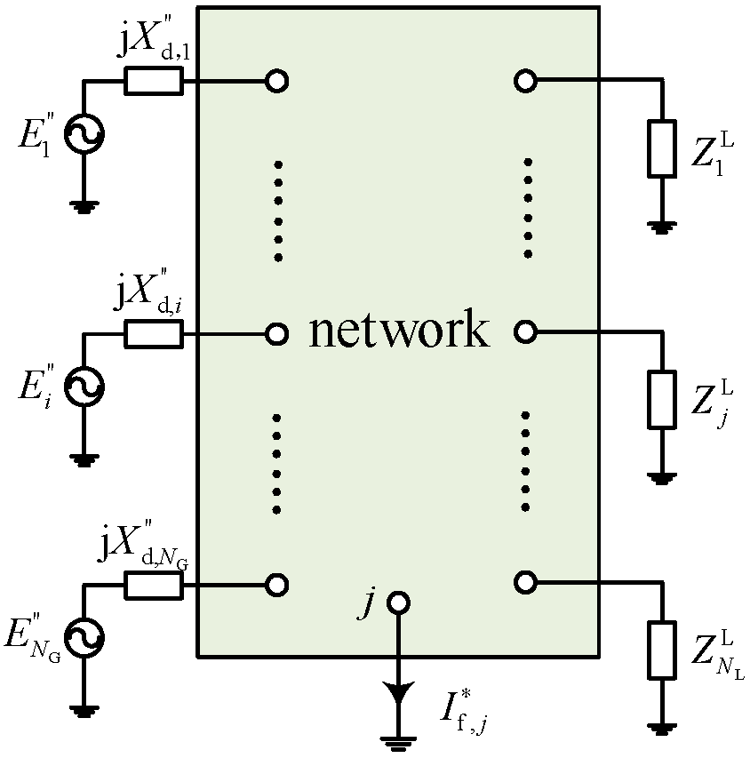
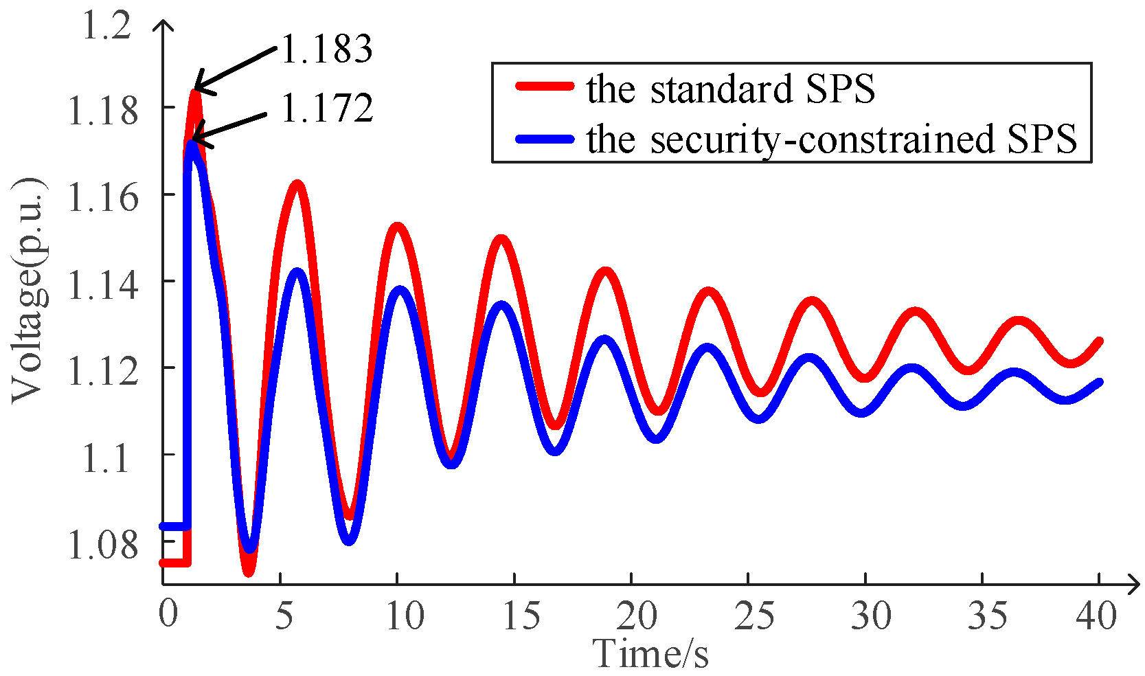
2.1. Voltage Support Requirements
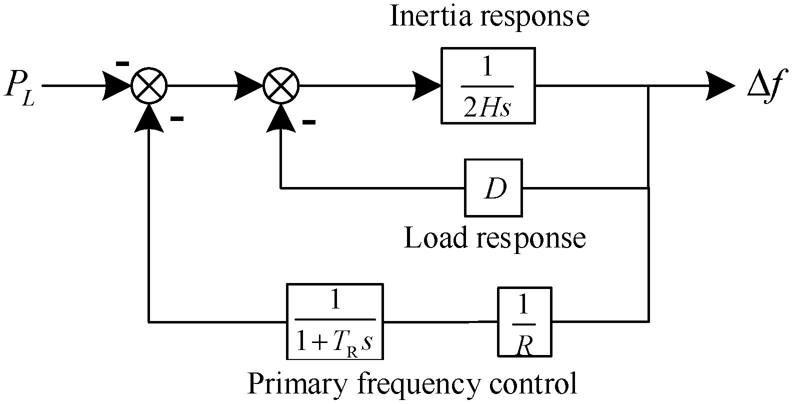
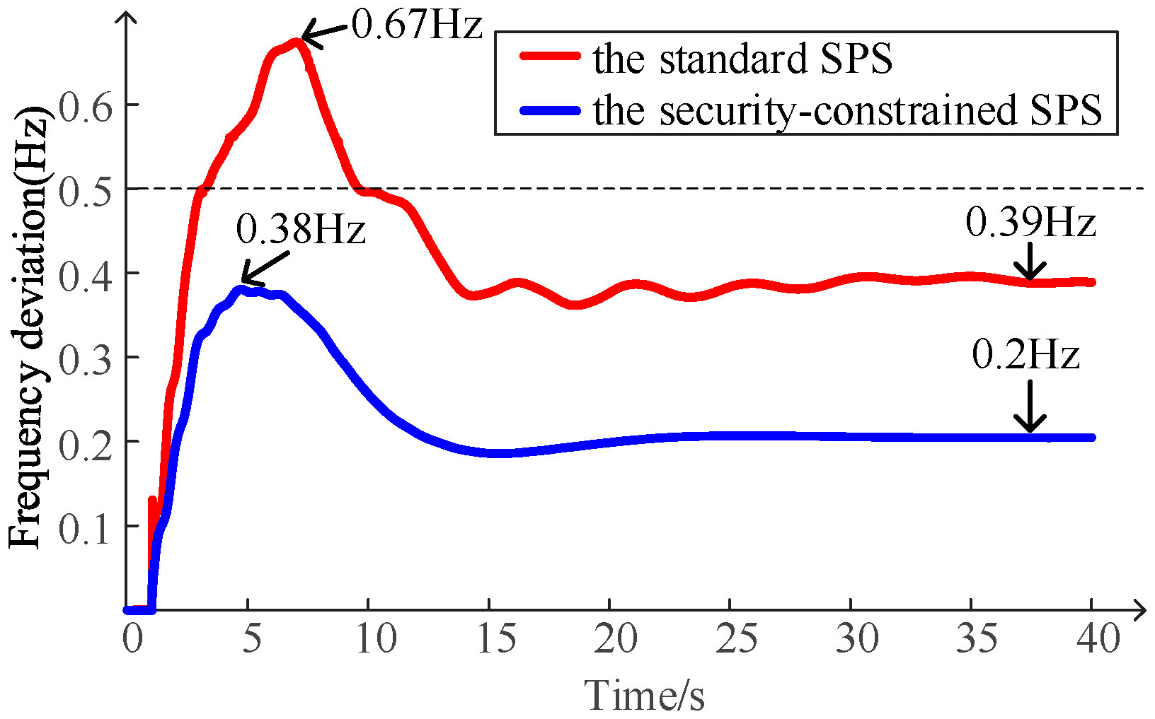
2.2. Frequency Support Requirements
3. Security-Constrained Sequential Production Simulation for Assessing Renewable Energy Absorption Capacity
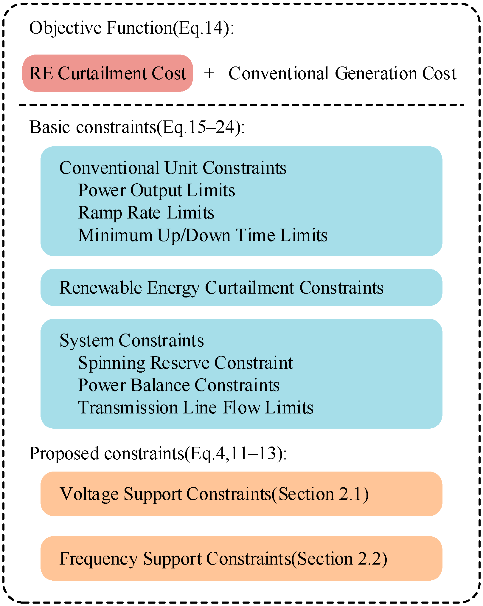
3.1. Objective Function
3.2. Startup and Shutdown Cost Constraints
3.3. Conventional Generator Unit Constraints
- (1)
- Power Output Limits
- (2)
- Ramp Rate Limits
- (3)
- Minimum Up/Down Time Limits
3.4. Renewable Energy Curtailment Constraints
3.5. System Constraints
- (1)
- Spinning Reserve Constraint
- (2)
- Power Balance Constraints
- (3)
- Transmission Line Flow Limits
- (4)
- Voltage Support Constraints
- (5)
- Frequency Support Constraints
4. Temporal Aggregation-Based Solution for Security-Constrained Sequential Production Simulation
4.1. Hierarchical Clustering-Based TA
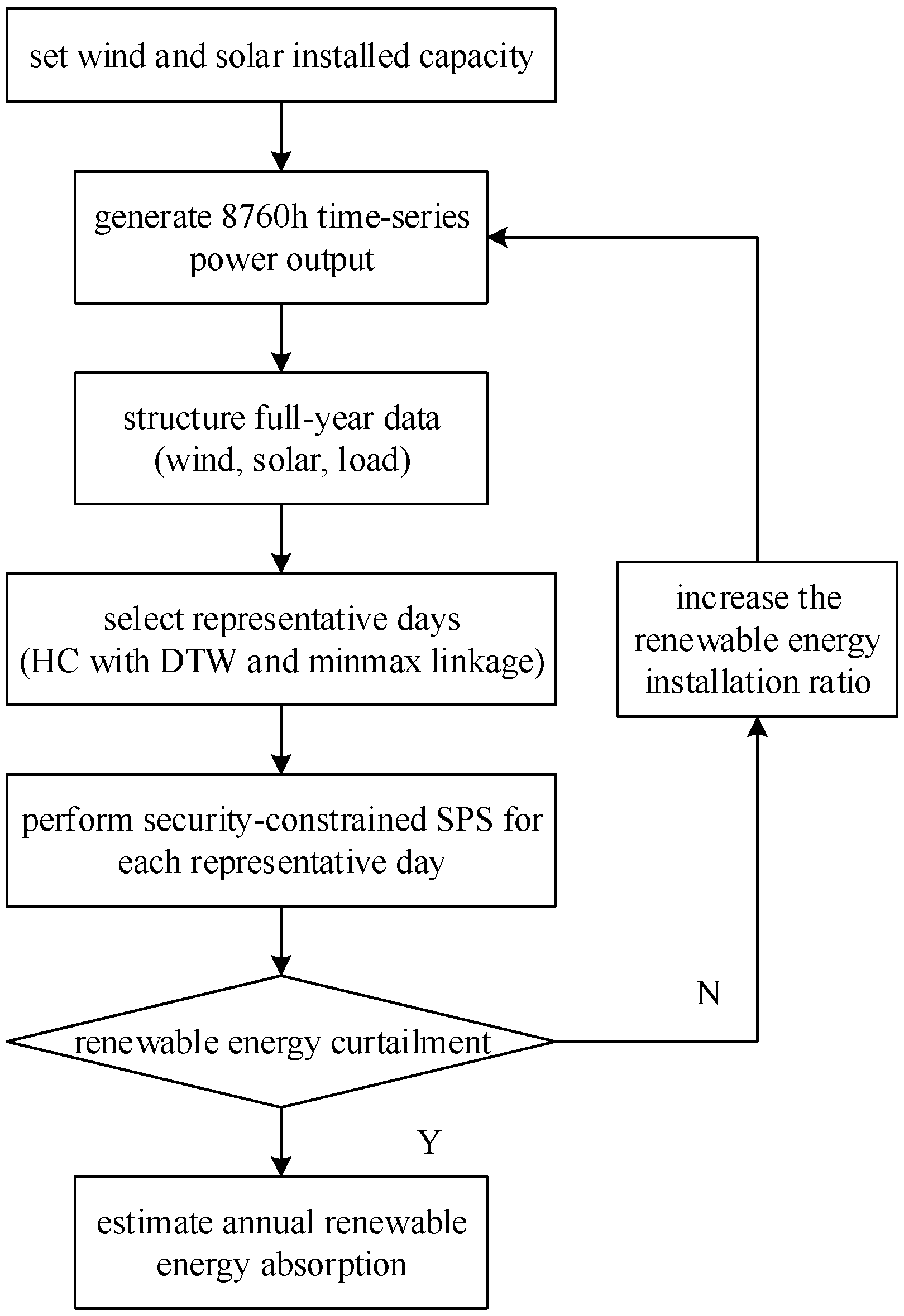
4.2. Solution Framework
- (1)
- Set wind and solar installed capacity.
- (2)
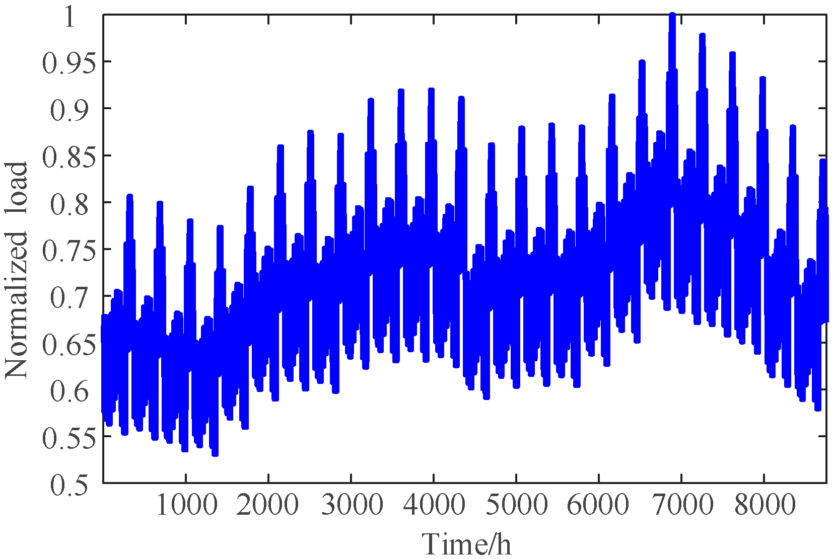
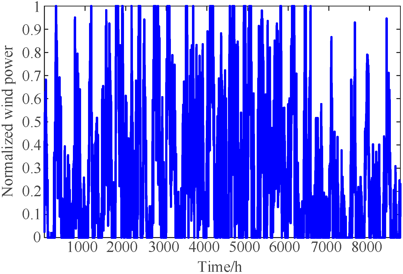
- Generate 8760 h time-series power output based on annual wind and solar generation characteristics.
- (3)
- Organize full-year data by structuring wind, solar, and load demand in a daily format.
- (4)
- Select representative days using HC with DTW and min-max linkage.
- (5)
- Perform security-constrained SPS for each representative day. If no renewable energy curtailment occurs, increase the renewable energy installation ratio and return to Step 2. Otherwise, statistically analyze renewable energy absorption.
- (6)
- Estimate annual renewable energy absorption by aggregating the weighted results of representative days.
5. Case Study
5.1. Case1: The IEEE 39-Bus System
- (1)
- Representative Day Selection
- (2)
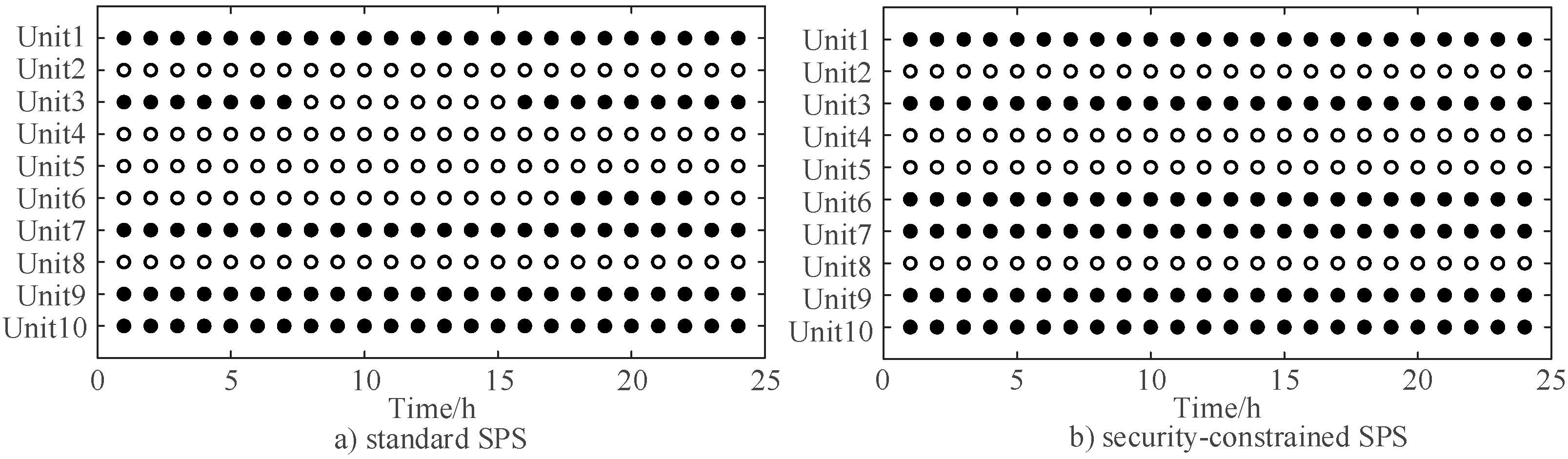
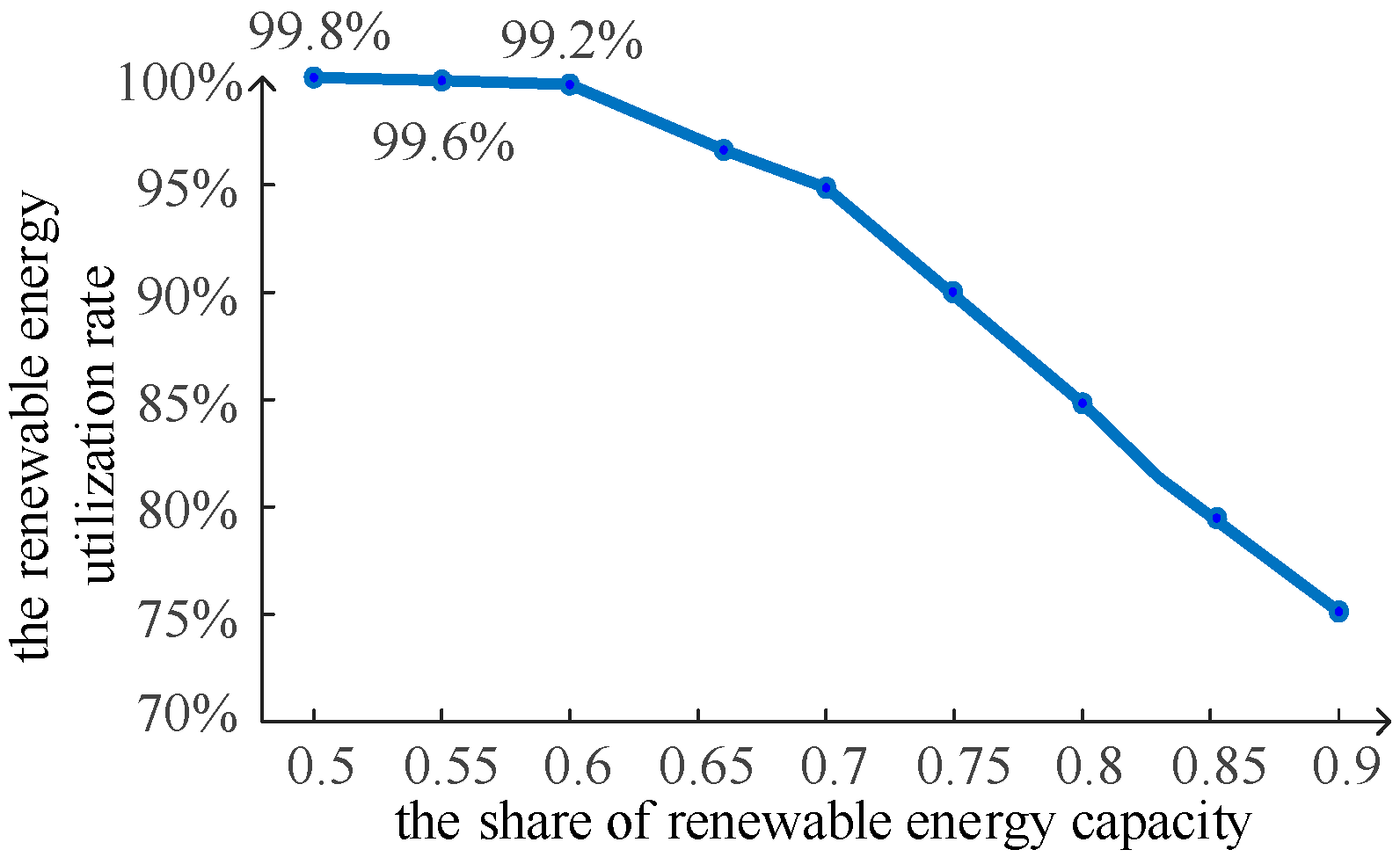
- Renewable Energy Absorption Assessment
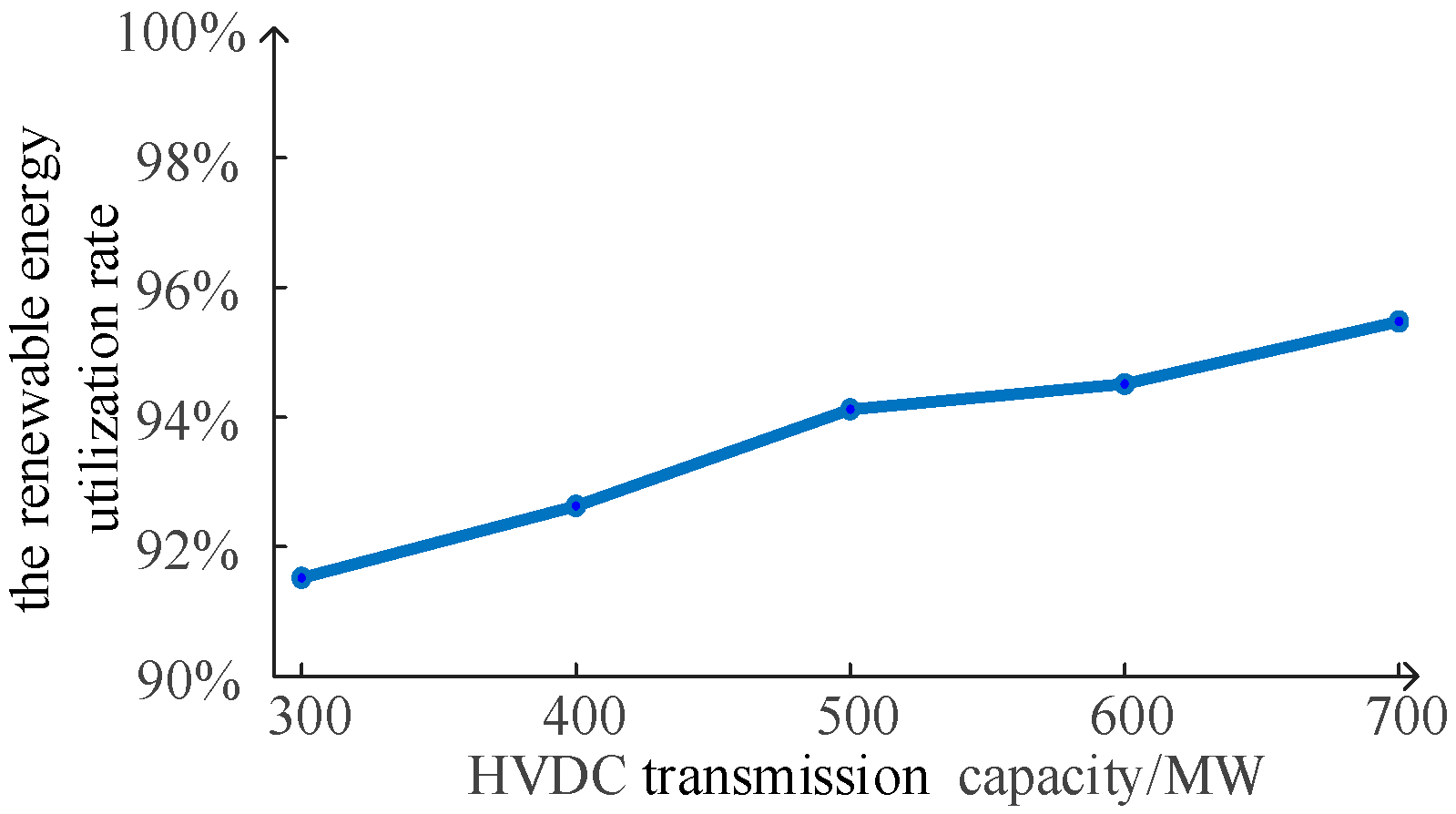
- (3)
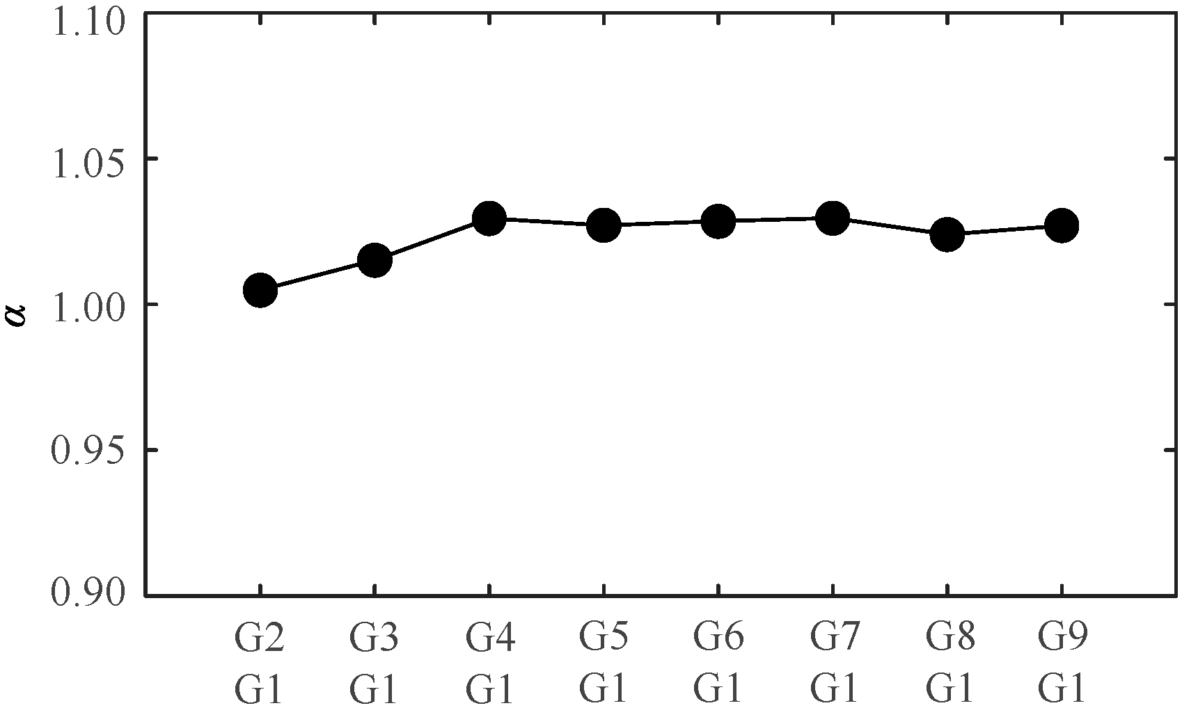
- Factors Improving Renewable Energy Absorption
5.2. Case2: The IEEE 68-Bus System
6. Conclusions
Author Contributions
Funding
Data Availability Statement
Conflicts of Interest
References
- IRENA. Renewable Energy Statistics 2024; International Renewable Energy Agency: Abu Dhabi, United Arab Emirates, 2024. [Google Scholar]
- Bird, L.; Lew, D.; Milligan, M.; Carlini, E.M.; Estanqueiro, A.; Flynn, D.; Gomez-Lazaro, E.; Holttinen, H.; Menemenlis, N.; Orths, A. Wind and solar energy curtailment: A review of international experience. Renew. Sustain. Energy Rev. 2016, 65, 577–586. [Google Scholar] [CrossRef]
- Li, P.; Sun, W.; Zhang, Z.; He, Y.; Wang, Y. Forecast of renewable energy penetration potential in the goal of carbon peaking and carbon neutrality in China. Sustain. Prod. Consum. 2022, 34, 541–551. [Google Scholar] [CrossRef]
- You, W.; Geng, Y.; Dong, H.; Wilson, J.; Pan, H.; Wu, R.; Sun, L.; Zhang, X.; Liu, Z. Technical and economic assessment of RES penetration by modelling China’s existing energy system. Energy 2018, 165, 900–910. [Google Scholar] [CrossRef]
- Zhang, D.; Mu, S.; Chan, C.C.; Zhou, G.Y. Optimization of renewable energy penetration in regional energy system. Energy Procedia 2018, 152, 922–927. [Google Scholar] [CrossRef]
- Bunodiere, A.; Lee, H.S. Renewable energy curtailment: Prediction using a logic-based forecasting method and mitigation measures in Kyushu, Japan. Energies 2020, 13, 4703. [Google Scholar] [CrossRef]
- Akeyo, O.M.; Patrick, A.; Ionel, D.M. Study of renewable energy penetration on a benchmark generation and transmission system. Energies 2020, 14, 169. [Google Scholar] [CrossRef]
- Memmel, E.; Schlüters, S.; Völker, R.; Schuldt, F.; Von Maydell, K.; Agert, C. Forecast of renewable curtailment in distribution grids considering uncertainties. IEEE Access 2021, 9, 60828–60840. [Google Scholar] [CrossRef]
- Egido, I.; Fernandez-Bernal, F.; Centeno, P.; Rouco, L. Maximum frequency deviation calculation in small isolated power systems. IEEE Trans. Power Syst. 2009, 24, 1731–1738. [Google Scholar] [CrossRef]
- Ahmadi, H.; Ghasemi, H. Security-constrained unit commitment with linearized system frequency limit constraints. IEEE Trans. Power Syst. 2014, 29, 1536–1545. [Google Scholar] [CrossRef]
- Teng, F.; Trovato, V.; Strbac, G. Stochastic scheduling with inertia-dependent fast frequency response requirements. IEEE Trans. Power Syst. 2015, 31, 1557–1566. [Google Scholar] [CrossRef]
- Paturet, M.; Markovic, U.; Delikaraoglou, S.; Vrettos, E.; Aristidou, P.; Hug, G. Stochastic unit commitment in low-inertia grids. IEEE Trans. Power Syst. 2020, 35, 3448–3458. [Google Scholar] [CrossRef]
- Zhang, Z.; Du, E.; Teng, F.; Zhang, N.; Kang, C. Modeling frequency dynamics in unit commitment with a high share of renew able energy. IEEE Trans. Power Syst. 2020, 35, 4383–4395. [Google Scholar] [CrossRef]
- Dai, J.; Tang, Y.; Wang, Q. Fast method to estimate maximum penetration level of wind power considering frequency cumulative effect. IET Gener. Transm. Distrib. 2019, 13, 1726–1733. [Google Scholar] [CrossRef]
- Wang, B.; Sun, H.; Zhao, B.; Wu, P.; Li, W.; Xu, S.; Chen, J. Calculation method of renewable maximum penetration considering frequency response of renewable energy. Electr. Power Syst. Res. 2024, 237, 110984. [Google Scholar] [CrossRef]
- Niu, S.; Zhang, Z.; Ke, X.; Zhang, G.; Huo, C.; Qin, B. Impact of renewable energy penetration rate on power system transient voltage stability. Energy Rep. 2022, 8, 487–492. [Google Scholar] [CrossRef]
- Lekshmi, J.D.; Rather, Z.H.; Pal, B.C. A new tool to assess maximum permissible solar PV penetration in a power system. Energies 2021, 14, 8529. [Google Scholar] [CrossRef]
- Li, C.; Zhang, D.; Liu, Z.; Xiong, Y.; Yu, T.; Gao, Z.; Miao, S. An Evaluation Method of Renewable Energy Resources’ Penetration Capacity of an AC-DC Hybrid Grid. Energies 2022, 15, 2550. [Google Scholar] [CrossRef]
- Wu, Y.; Zhou, H.; Zhang, C.; Liu, S.; Chen, Z. Multi-scenario renewable energy absorption capacity assessment method based on the attention-enhanced time convolutional network. Front. Energy Res. 2024, 12, 1347553. [Google Scholar] [CrossRef]
- Dalala, Z.; Al-Omari, M.; Al-Addous, M.; Bdour, M.; Al-Khasawneh, Y.; Alkasrawi, M. Increased renewable energy penetration in national electrical grids constraints and solutions. Energy 2022, 246, 123361. [Google Scholar] [CrossRef]
- Zhou, D.; Zhang, Q.; Dan, Y.; Guo, F.; Qi, J.; Teng, C.; Zhu, H. Research on renewable-energy accommodation-capability evaluation based on time-series production simulations. Energies 2022, 15, 6987. [Google Scholar] [CrossRef]
- Kotzur, L.; Markewitz, P.; Robinius, M.; Stolten, D. Impact of different time series aggregation methods on optimal energy system design. Renew. Energy 2018, 117, 474–487. [Google Scholar] [CrossRef]
- Hoffmann, M.; Kotzur, L.; Stolten, D.; Robinius, M. A Review on Time Series Aggregation Methods for Energy System Models. Energies 2020, 13, 641. [Google Scholar] [CrossRef]
- Gke, L.; Kendziorski, M. Adequacy of time-series reduction for renewable energy systems. Energy 2022, 238, 121701. [Google Scholar] [CrossRef]
- Teichgraeber, H.; Brandt, A.R. Time-series aggregation for the optimization of energy systems: Goals, challenges, approaches, and opportunities. Renew. Sustain. Energy Rev. 2022, 157, 111984. [Google Scholar] [CrossRef]
- Poncelet, K.; Höschle, H.; Delarue, E.; Virag, A.; D’haeseleer, W. Selecting representative days for capturing the implications of integrating intermittent renewables in generation expansion planning problems. IEEE Trans. Power Syst. 2016, 32, 1936–1948. [Google Scholar] [CrossRef]
- Shair, J.; Li, H.; Hu, J.; Xie, X. Power system stability issues, classifications and research prospects in the context of high-penetration of renewables and power electronics. Renew. Sustain. Energy Rev. 2021, 145, 111111. [Google Scholar] [CrossRef]
- Anderson, P.M.; Mirheydar, M. A low-order system frequency response model. IEEE Trans. Power Syst. 1990, 5, 720–729. [Google Scholar] [CrossRef]
- Bevrani, H. Robust Power System Frequency Control; Springer: Berlin/Heidelberg, Germany, 2009. [Google Scholar]
- Bien, J.; Tibshirani, R. Hierarchical clustering with prototypes via minimax linkage. J. Am. Stat. Assoc. 2011, 106, 1075–1084. [Google Scholar] [CrossRef]
- Canizares, C.; Fernandes, T.; Geraldi, E.; Gerin-Lajoie, L.; Gibbard, M.; Hiskens, I.; Kersulis, J.; Kuiava, R.; Lima, L.; DeMarco, F.; et al. Benchmark Models for the Analysis and Control of Small-Signal Oscillatory Dynamics in Power Systems. IEEE Trans. Power Syst. 2017, 32, 715–722. [Google Scholar] [CrossRef]
- Zhuo, Z.; Zhang, N.; Yang, J.; Kang, C.; Smith, C.; O’Malley, M.J.; Kroposki, B. Transmission expansion planning test system for AC/DC hybrid grid with high variable renewable energy penetration. IEEE Trans. Power Syst. 2019, 35, 2597–2608. [Google Scholar] [CrossRef]
- Available online: https://ww2.mathworks.cn/help/sps/ug/ieee-39-bus-system.html (accessed on 24 May 2025).
- GB/T 19963.1-2021; Technical Specification for Connecting Wind Farm to Power System-Part 1: On Shore Wind Power. National Standardization Administration of China: Beijing, China, 2021. (In Chinese)
- GB/T 19964-2024; Technical Requirements for Connecting Photovoltaic Station to Power System. National Standardization Administration of China: Beijing, China, 2024. (In Chinese)
- GB/T 15945-2008; Power Quality—Frequency Deviation for Power System. National Standardization Administration of China: Beijing, China, 2008. (In Chinese)
- Abhinav Kumar, S.; Pal, B.C. IEEE PES Task Force on Benchmark Systems for Stability Controls: Report on the 68-Bus, 16-Machine, 5-Area System. 2013. Available online: https://www.researchgate.net/publication/311680574_IEEE_PES_Task_Force_on_Benchmark_Systems_for_Stability_Controls_Report_on_the_68-Bus_16-Machine_5-Area_System (accessed on 24 May 2025).


| Methods | RMSE |
|---|---|
| HC with DTW and min-max linkage | 0.0238 |
| HC with ED and ward linkage | 0.0486 |
| k-means | 0.0317 |
| Month | The Available Generation Power of RES | Renewable Energy Absorption Using Standard SPS | Renewable Energy Absorption | ||
|---|---|---|---|---|---|
| Security-Constrained SPS Without TA | Security-Constrained SPS with TA | Related Error | |||
| January | 4955.22 | 4955.22 | 4939.04 | 4954.66 | 0.32% |
| February | 5182.58 | 5182.58 | 5167.06 | 5174.17 | 0.14% |
| March | 8094.10 | 8094.10 | 7835.93 | 8024.94 | 2.41% |
| April | 7526.10 | 7526.10 | 7225.50 | 7441.94 | 2.99% |
| May | 8143.92 | 8143.92 | 7976.64 | 8084.04 | 1.35% |
| June | 8420.04 | 8420.04 | 8188.83 | 8329.42 | 1.72% |
| July | 9297.89 | 9297.89 | 8874.79 | 9068.78 | 2.19% |
| August | 7874.09 | 7874.09 | 7701.22 | 7860.44 | 2.07% |
| September | 7557.15 | 7557.15 | 7262.77 | 7472.09 | 2.88% |
| October | 4479.67 | 4479.67 | 4455.42 | 4479.67 | 0.55% |
| November | 5083.13 | 5083.13 | 5077.67 | 5080.60 | 0.06% |
| December | 5042.09 | 5042.09 | 5035.53 | 5042.09 | 0.13% |
| Annual | 81,655.99 | 81,655.99 | 79,740.40 | 81,012.84 | 1.60% |
| t | Standard SPS | Security-Constrained SPS | ||||||||||
|---|---|---|---|---|---|---|---|---|---|---|---|---|
| Unit 1 | Unit 3 | Unit 6 | Unit 7 | Unit 9 | Unit 10 | Unit 1 | Unit 3 | Unit 6 | Unit 7 | Unit 9 | Unit 10 | |
| 1 | 5.08 | 7.25 | off | 6.38 | 8.65 | 11.00 | 5.08 | 7.25 | 3.26 | 3.12 | 8.65 | 11.00 |
| 2 | 5.08 | 7.25 | off | 4.77 | 8.65 | 11.00 | 5.08 | 6.16 | 3.21 | 3.12 | 8.19 | 11.00 |
| 3 | 5.08 | 7.25 | off | 3.46 | 8.65 | 11.00 | 5.08 | 5.12 | 3.18 | 3.12 | 7.95 | 11.00 |
| 4 | 5.08 | 7.25 | off | 3.61 | 8.65 | 11.00 | 5.08 | 5.86 | 2.74 | 3.12 | 7.79 | 11.00 |
| 5 | 5.08 | 7.25 | off | 5.82 | 8.65 | 11.00 | 5.08 | 6.53 | 3.48 | 3.12 | 8.59 | 11.00 |
| 6 | 5.08 | 7.25 | off | 3.33 | 8.65 | 11.00 | 3.24 | 2.18 | 7.01 | 3.22 | 8.65 | 11.00 |
| 7 | 5.08 | 4.71 | off | 3.78 | 8.65 | 11.00 | 1.52 | 2.18 | 7.01 | 4.68 | 8.65 | 11.00 |
| 8 | 5.08 | off | off | 7.30 | 8.65 | 11.00 | 1.52 | 2.18 | 7.01 | 3.85 | 8.65 | 11.00 |
| 9 | 5.08 | off | off | 7.78 | 8.65 | 11.00 | 1.52 | 2.18 | 7.01 | 4.52 | 8.65 | 11.00 |
| 10 | 5.08 | off | off | 5.52 | 8.65 | 11.00 | 1.52 | 2.18 | 7.01 | 3.16 | 8.65 | 11.00 |
| 11 | 5.08 | off | off | 7.10 | 8.65 | 11.00 | 2.92 | 2.18 | 3.96 | 3.12 | 8.65 | 11.00 |
| 12 | 5.08 | off | off | 7.99 | 8.65 | 11.00 | 5.08 | 2.32 | 2.55 | 3.12 | 8.65 | 11.00 |
| 13 | 5.08 | off | off | 3.12 | 8.28 | 11.00 | 3.40 | 2.18 | 2.55 | 3.12 | 5.24 | 11.00 |
| 14 | 5.08 | off | off | 3.12 | 8.38 | 11.00 | 2.58 | 2.18 | 2.55 | 3.12 | 6.15 | 11.00 |
| 15 | 5.08 | off | off | 6.13 | 8.65 | 11.00 | 4.34 | 2.18 | 2.55 | 3.12 | 7.68 | 11.00 |
| 16 | 5.08 | 4.71 | off | 4.06 | 8.65 | 11.00 | 5.08 | 3.10 | 2.55 | 3.12 | 8.65 | 11.00 |
| 17 | 5.08 | 7.25 | off | 3.18 | 8.65 | 11.00 | 4.07 | 2.67 | 5.65 | 3.12 | 8.65 | 11.00 |
| 18 | 5.08 | 7.25 | 5.53 | 3.96 | 8.65 | 11.00 | 5.08 | 7.02 | 6.59 | 3.12 | 8.65 | 11.00 |
| 19 | 5.08 | 7.25 | 8.50 | 5.81 | 8.65 | 11.00 | 5.08 | 7.25 | 8.50 | 5.81 | 8.65 | 11.00 |
| 20 | 5.08 | 7.25 | 7.01 | 4.23 | 8.65 | 11.00 | 5.08 | 6.22 | 7.33 | 4.94 | 8.65 | 11.00 |
| 21 | 5.08 | 7.25 | 7.15 | 4.94 | 8.65 | 11.00 | 5.08 | 7.25 | 7.15 | 4.94 | 8.65 | 11.00 |
| 22 | 5.08 | 7.25 | 5.53 | 4.55 | 8.65 | 11.00 | 5.08 | 7.03 | 7.01 | 3.28 | 8.65 | 11.00 |
| 23 | 5.08 | 7.25 | off | 7.48 | 8.65 | 11.00 | 5.08 | 5.67 | 5.94 | 3.12 | 8.65 | 11.00 |
| 24 | 5.08 | 7.25 | off | 4.68 | 8.65 | 11.00 | 5.08 | 2.99 | 5.82 | 3.12 | 8.65 | 11.00 |
| No. | Representative Day | Days Included |
|---|---|---|
| 1 | 148 | 63 |
| 2 | 330 | 25 |
| 3 | 55 | 2 |
| 4 | 168 | 13 |
| 5 | 146 | 3 |
| 6 | 167 | 9 |
| 7 | 290 | 21 |
| 8 | 186 | 9 |
| 9 | 177 | 2 |
| 10 | 154 | 9 |
| 11 | 316 | 4 |
| 12 | 179 | 5 |
| 13 | 212 | 1 |
| 14 | 299 | 6 |
| 15 | 352 | 5 |
| 16 | 38 | 17 |
| 17 | 357 | 7 |
| 18 | 294 | 8 |
| 19 | 268 | 9 |
| 20 | 335 | 8 |
| 21 | 286 | 73 |
| 22 | 111 | 24 |
| 23 | 235 | 24 |
| 24 | 78 | 9 |
| 25 | 207 | 9 |
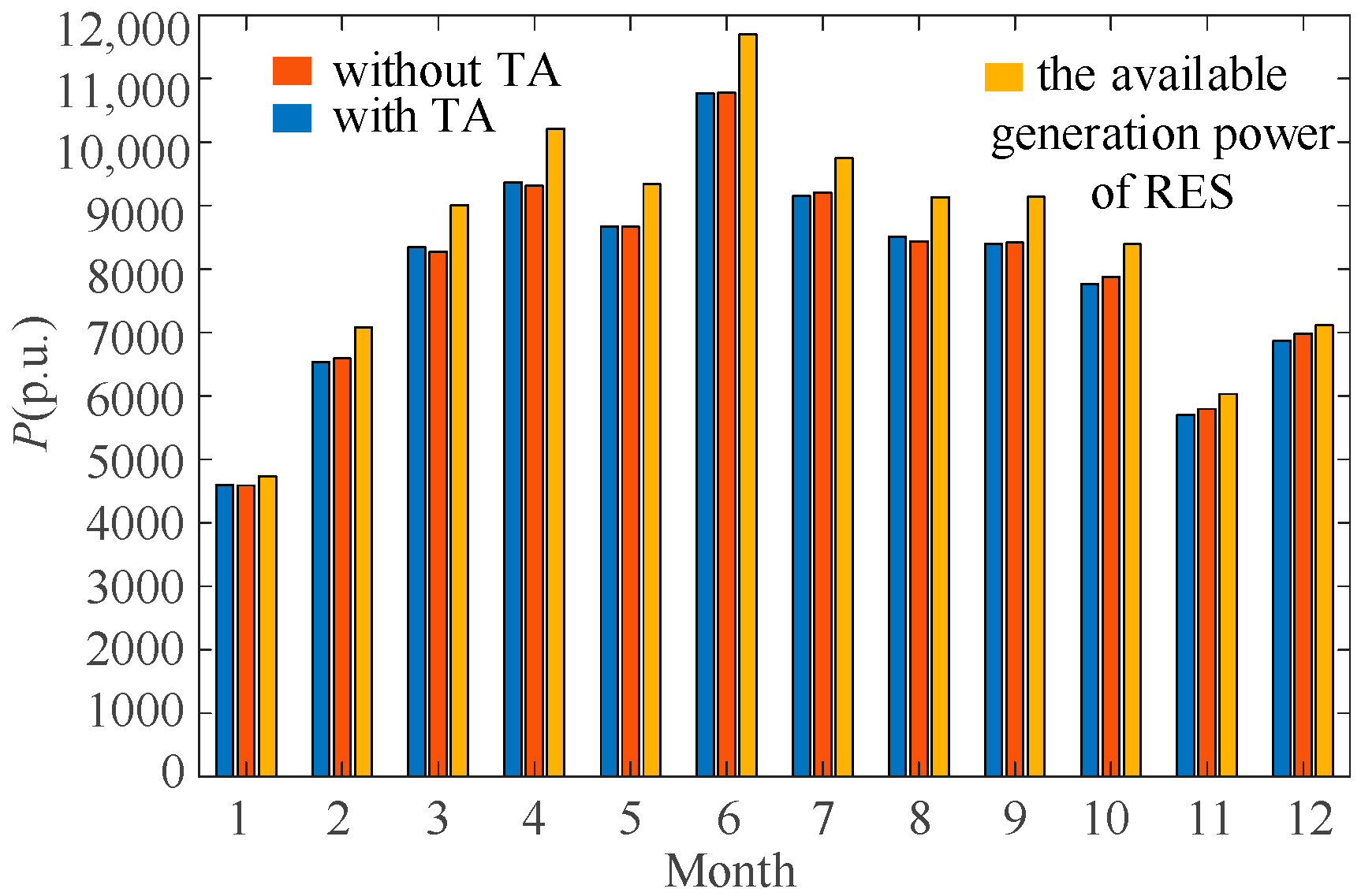
| Month | The Available Generation Power of RES | Renewable Energy Absorption | ||
|---|---|---|---|---|
| Security-Constrained SPS Without TA | Security-Constrained SPS with TA | Related Error | ||
| January | 4731.35 | 4588.71 | 4594.22 | 0.12% |
| February | 7077.31 | 6590.42 | 6533.33 | 0.81% |
| March | 9006.41 | 8269.12 | 8342.46 | 0.81% |
| April | 10,210.21 | 9308.10 | 9362.00 | 0.53% |
| May | 9334.78 | 8664.07 | 8669.02 | 0.05% |
| June | 11,696.22 | 10,775.16 | 10,765.99 | 0.08% |
| July | 9747.33 | 9204.93 | 9148.44 | 0.58% |
| August | 9127.13 | 8430.92 | 8505.85 | 0.82% |
| September | 9137.34 | 8413.78 | 8399.01 | 0.16% |
| October | 8388.05 | 7876.97 | 7764.96 | 1.34% |
| November | 6034.20 | 5792.50 | 5704.11 | 1.46% |
| December | 7112.83 | 6979.10 | 6869.06 | 1.55% |
| Annual | 101,603.18 | 94,893.77 | 94,658.44 | 0.23% |
Disclaimer/Publisher’s Note: The statements, opinions and data contained in all publications are solely those of the individual author(s) and contributor(s) and not of MDPI and/or the editor(s). MDPI and/or the editor(s) disclaim responsibility for any injury to people or property resulting from any ideas, methods, instructions or products referred to in the content. |
© 2025 by the authors. Licensee MDPI, Basel, Switzerland. This article is an open access article distributed under the terms and conditions of the Creative Commons Attribution (CC BY) license (https://creativecommons.org/licenses/by/4.0/).
Share and Cite
Feng, Z.; Zhang, Y.; Liu, J.; Wang, T.; Cai, P.; Xu, L. Analysis of Renewable Energy Absorption Potential via Security-Constrained Power System Production Simulation. Energies 2025, 18, 2994. https://doi.org/10.3390/en18112994
Feng Z, Zhang Y, Liu J, Wang T, Cai P, Xu L. Analysis of Renewable Energy Absorption Potential via Security-Constrained Power System Production Simulation. Energies. 2025; 18(11):2994. https://doi.org/10.3390/en18112994
Chicago/Turabian StyleFeng, Zhihui, Yaozhong Zhang, Jiaqi Liu, Tao Wang, Ping Cai, and Lixiong Xu. 2025. "Analysis of Renewable Energy Absorption Potential via Security-Constrained Power System Production Simulation" Energies 18, no. 11: 2994. https://doi.org/10.3390/en18112994
APA StyleFeng, Z., Zhang, Y., Liu, J., Wang, T., Cai, P., & Xu, L. (2025). Analysis of Renewable Energy Absorption Potential via Security-Constrained Power System Production Simulation. Energies, 18(11), 2994. https://doi.org/10.3390/en18112994