Numerical Study of the Condenser of a Small CO₂ Refrigeration Unit Operating Under Supercritical Conditions

Abstract

The paper presents a numerical analysis of a tube-in-tube condenser of a small refrigeration system. One of the challenges in designing such units is to reduce their dimensions while maintaining the highest possible cooling capacity, so the research presented here focuses on the search for and impact of the appropriate flow conditions of these two fluids on condenser performance. The refrigerant is supercritical CO₂, which is cooled by water. Thermal-flow simulations were performed for eight CO₂ inlet velocities in the range of 1–8 m/s, and four cooling water velocities of 0.5–2 m/s. The main parameters of the exchanger operation were analyzed: heat transfer coefficient, Nusselt number, overall heat transfer coefficient, and friction factor, which were compared with selected correlations. The results showed that the condenser achieves the highest power for the highest water velocities (2 m/s) and CO₂ (8 m/s), i.e., over 1000 W, which corresponds to a heat flux on the tube surface of approx. 2.6 × 10⁵ W/m² and a heat transfer coefficient of approx. 4700 W/m²K. One of the most important conclusions is the discovery of a significant effect of water velocity on heat transfer from the CO₂ side—an increase in water velocity from 0.5 m/s to 2 m/s results in an increase in the heat transfer coefficient sCO₂ by over 60%, with the same Re number. The implication of this study is to show the possibility of adjusting and selecting condenser parameters over a wide range of capacities, just by changing the fluid velocity.

1. Introduction

Refrigeration devices are used in many areas of life, from household appliances such as refrigerators or tumble dryers, through air conditioning in vehicles, to manufacturing processes such as packaging and storing food, medicines, chemical reagents, or biological samples. For this reason, scientists are conducting more and more research into modifying refrigeration systems and using new refrigerants [1,2]. Nowadays, the most popular refrigerants are chlorofluorocarbons (CFCs) and hydrochlorofluorocarbons (HCFCs). Unfortunately, their use in refrigeration technologies, to a greater or lesser extent, causes degeneration of the ozone layer and contributes to global warming. In addition, these substances are often toxic and pose a risk to users in case of a leak or accident [2,3]. Therefore, more and more efforts are being put into the search for alternative refrigerants, where natural substances such as water (R718) [4], ammonia (R717) [5], propane (R290), isobutane (R600a), and carbon dioxide (R744) [6] can be substitutes for CFCs and HCFCs in many applications [7]. Among these, CO₂ has attracted the most attention from researchers because of its safe use, non-flammability and non-toxicity, availability, low cost, and environmental benefits. Its emissions do not affect the degradation of the ozone layer, making its ODP (Ozone Depletion Potential) value 0, while its global warming potential (GWP) is one and is the reference point on this scale. In the past, CO₂ had already been used as a refrigerant until about the 1940s. However, it was replaced by CFCs and HCFCs due to its lower efficiency in conventional refrigeration systems using vapor compression operating at lower pressures [1,2].

The main feature that distinguishes CO₂ from other refrigerants is its critical parameters—high pressure of 7.39 MPa and low temperature of 30.98 °C. For this reason, refrigeration circuits using CO₂ as a refrigerant are constructed as transcritical circuits, since CO₂ will be in a supercritical state in the condenser of the system [8].

Many studies of supercritical systems using CO₂ can be found in the literature, but they are mostly for units with cooling capacities above 2 kW. One point of reference for the results presented in this article is experimental studies of sCO₂ (supercritical CO₂) in tube-in-tube heat exchangers. Liao and Zhao [9] conducted experimental studies of heat transfer coefficients in micro and small channels as a function of temperature, diameters, pressures, and mass fluxes. They studied pipe diameters: 0.5 mm, 0.7 mm, 1.1 mm, 1.4 mm, 1.55 mm, and 2.16 mm, at pressures ranging from 7.4 to 12 MPa and mass fluxes ranging from 0.02 to 0.2 kg/min. The study showed a variation in the heat transfer coefficient around the critical temperature, which reached a maximum for temperatures slightly higher than the critical temperature. They proved that there is a significant decrease in the Nusselt number for microchannels with a diameter of less than 1.1 mm, and also determined a new correlation of the Nusselt number for micro and small channels. Dang and Hihara [10] performed experimental studies of the cooling of sCO₂ in channels of different diameters: 1 mm, 2 mm, 4 mm, and 6 mm in the pressure range of 8–10 MPa, and studied the effects of mass flux, pressures and temperatures on the heat transfer coefficient and Nusselt number. Studies have shown that the heat transfer coefficient is directly proportional to the mass flow, and a sudden increase occurs around the critical temperature. A study of the effect of pressure, on the other hand, found that an increase in CO₂ pressure decreases the coefficient. In addition, they gave a new Nusselt number correlation model, as standard correlations proved inaccurate. Zhang et al. [11] conducted experimental studies of sCO₂ cooling in pipes with diameters: 4.12 mm, 5.95 mm, 7.64 mm, and 9.44 mm with a length of 1 m each, where they examined the effects of diameter, mass flow, and pressure on the heat transfer coefficient. They showed that the heat transfer coefficient assumed the largest values for the pipe with the smallest diameter among those tested. In line with other studies, they also showed that an increase in pressure decreases the value of the heat transfer coefficient and that it is directly proportional to the mass flow of the medium. Lei et al. [12] performed an experimental study on the effect of the position of a microchannel with a diameter of 1 mm for vertical and horizontal sCO₂ flow and considered the effect of buoyancy forces on sCO₂ cooling and heat transfer efficiency. They showed that in vertical microchannels, sCO₂ heat transfer is more efficient because the wall temperature is more homogeneous, which improves the heat transfer effectiveness of the pipe. Wahl et al. [13] performed a series of experimental studies assuming cooling of a pipe with a fixed diameter of 2 mm and a length of 1.2 m and checking the effect of mass flow, pressure, and water temperature on the heat transfer coefficient. The conclusions of the study are consistent with others presented above—the largest changes in parameters take place around the critical temperature, and the heat transfer coefficient is directly proportional to the mass flow, while an increase in pressure sCO₂ decreases its value.

Experimental studies provide quantitative information on heat transfer and flow resistance in channels with sCO₂, but the velocity and temperature fields and flow turbulence cannot be analyzed from them. This gap is filled by numerical studies, the results of which provide data on the effects of pressure, mass flux, and temperature of the coolant on the cooling performance of sCO₂.

Tu and Zeng [14] performed numerical calculations using ANSYS FLUENT 16.0 software in which they investigated the effects of the diameter and geometry of circular and semicircular minichannels with diameters of 0.5 mm, 1 mm, and 2 mm, on the heat transfer coefficient during sCO₂ cooling, for constant inlet velocities of 1–2 m/s and mass flows of 800–1200 kg/m²s, in the inlet temperature range 27–67 °C and at a constant pressure of 9 MPa. They assumed boundary conditions on the wall as a constant heat flux of 6, 12, and 24 kW/m² and used the SST k-omega turbulence model. The study showed that in circular channels the heat transfer coefficient is higher than in semicircular ones, reaching a maximum near the critical temperature, and that the smaller the diameter of the duct, the greater the convective heat transfer, but the flow resistance and pressure drop increase. Du et al. [15] numerically investigated the cooling of sCO₂ in a 6 mm-diameter pipe using various turbulence models: standard k-ε, RNG k-ε, Reynolds Stress Model (RSM), and six models for low Reynolds number. They proved that all the models used were able to faithfully reproduce the thermal and flow characteristics of sCO₂ cooling, among which the low Reynolds number Lam–Bremhorst (LB) model, combined with k-ε and with an improved boundary layer model, best reproduced the experimental results. Wang et al. [16] performed a series of numerical studies to investigate the effect of pipe diameter on sCO₂ heat transfer. They performed numerical simulations for duct diameters from 1 to 6 mm, taking gravity into account, for pressures of 8–10 MPa, inlet temperatures of 330–350 K, and wall heat fluxes of 12–42 kW/m². The numerical model presented in the paper effectively predicts the heat transfer coefficient using the standard k-ε turbulence model with an enhanced wall layer model (EWT—Enhanced Wall Treatment). The study showed that despite maintaining a constant heat flux on the outer wall of the pipe, the actual heat flux on the inner surface is strongly inhomogeneous—its maximum value occurs on the upper surface of the pipe, and its minimum on the lower surface. The thermophysical properties of CO₂, such as density, thermal conductivity, and viscosity, have a significant effect on the heat transfer process, especially near the pseudo-critical temperature, which generally leads to the intensification of convective phenomena when the temperature increases. Xiang et al. [17] numerically studied the heat transfer of sCO₂ in pipes with diameters of 2, 4, and 6 mm. They assumed boundary conditions in which the mass flow at the inlet is 100 to 300 kg/m²s, the initial temperature of the fluid is 340.15 K, the pressure is 8 MPa, and a constant heat flux is applied to the pipe walls. They showed that the heat transfer coefficient is higher on the top surface of the pipe than on the bottom, due to the buoyancy effect. Higher heat flux amplifies this effect, leading to larger temperature differences between the top and bottom of the pipe. The larger diameter of the pipe also increases the buoyancy effect but reduces the overall cooling efficiency of sCO₂. The model was verified by comparing numerical results with experimental data, achieving a maximum error of 13.5%.

This paper attempts to numerically investigate the influence of the flow parameters of the condenser of a small refrigeration unit on its performance, where the effect of fluid velocities on friction factors and heat transfer is presented and discussed. By changing the velocities of the cooling water as well as the supercritical CO₂, the highest values of the exchanged heat flux have been searched for, while keeping the geometry of the heat exchanger constant. The novelty of the study found that changing the cooling water velocity causes a significant change in the Nu number and friction factor on the CO₂ side.

2. Thermophysical Properties of sCO₂

CO₂ heated and compressed above a critical point (sCO₂) rapidly changes its thermal and physical properties, which generally has a positive effect on heat transfer [2]. The density of sCO₂ is highly dependent on pressure and temperature. A phase change from liquid to supercritical at the same pressure results in a significant decrease in density, leading to a decrease in flow resistance. Figure 1a shows that the density decreases with an increase in temperature, while at higher temperatures (above 60 °C), it changes slightly [3]. Dynamic viscosity sCO₂ also decreases with increasing temperature and, like density, from about 60 °C onward, changes very little so that it can be taken as a constant value (Figure 1b) [18]. Specific heat at constant pressure is equally strongly dependent on the temperature and pressure of the fluid. The transition of the substance to a supercritical state causes its rapid growth, which reaches a maximum near the critical temperature (Figure 1c). As the pressure increases, the maximum values of specific heat decrease, which has a significant impact on the choice of parameters of the refrigeration circuit [2,3]. The thermal conductivity of sCO₂ forms a local maximum for p = 8 MPa near the critical point, and then decreases with increasing temperature (Figure 1d) [18]. A similar maximum of thermal conductivity is observed for higher pressures, but its value is increasingly smaller.

3. Materials and Methods

3.1. Geometrical Model

The main purpose of the numerical calculations was to determine the heat-flow characteristics of supercritical CO₂ in a tube-in-tube condenser for a small refrigeration system. The design of a small refrigeration system assumes that all components, including the exchanger, must be as small as possible while maintaining the assumed cooling power. A tube-in-tube heat exchanger was chosen for the analysis because of its relatively simple design and the low price of its manufacture. All numerical tests were performed for the same heat exchanger geometry, the dimensions of which are given in Figure 2.

3.2. Numerical Model and Boundary Conditions

Numerical simulations were performed using Ansys CFX 2025 R1 software. Since the geometry under study is axisymmetric, instead of using a full pipe, a slice with an opening angle of 20° and a length of 400 mm was used (Figure 3). This approach to the problem reduces the size of the computational mesh, which reduces the calculation time while maintaining high accuracy, and is widely used by other researchers [19,20,21]. Figure 3 also shows the computational domains and boundary conditions on the domain walls. The geometry slice under consideration consists of 3 domains: water (green in Figure 3), copper wall (brown in Figure 3), and CO₂ (blue in Figure 3).

A symmetry boundary condition was imposed on the side walls of the slice in each domain. The flow in the exchanger is counterflow; therefore, the fluid inlets are on opposite sides of the geometry.

Table 1. Boundary conditions in fluid and solid domains.

Domain	Boundary Condition	Parameter	Value
sCO2 (fluid domain) Reference pressure 10 MPa	Inlet	Temperature	353 K
		Velocity	1, 2, 3, 4, 5, 6, 7, 8 m/s
	Outlet	Average static pressure	0 Pa
Copper (solid domain)	Domain Interface 1
	Domain Interface 2
sCO2 (fluid domain)	Inlet	Temperature	293 K
		Velocity	0.5, 1, 1.5, 2 m/s
	Outlet	Average static pressure	0 Pa

shows the details of all the boundary conditions. For water, the reference pressure was 1 bar, and for sCO₂ it was 10 MPa. For such pressure, a real gas property table (RGP Table) was generated from the NIST MINI-REFPROP v9.5 database in the temperature range from 273 to 373 K. Due to the low variability of the physical parameters close to the critical values for a pressure of 10MPa, a temperature step of 1 °C was assumed in the RPG table. The parameters at the inlet of the inner pipe were chosen so that CO₂ at the outlet is always in a supercritical state. The inlet temperature of CO₂ in each case was the same at 353 K; only the velocity range at the inlet changed, which was from 1 to 8 m/s. The walls of the pipe were the domain boundary, for which the heat transfer coefficient and heat flux were the resulting values. The cooling water at the inlet, in all cases, has a temperature of 293 K and a variable velocity in the range of 0.5–2 m/s.

3.3. Turbulence Model

For the simulations, the SST k-ω (shear stress transport) turbulence model was chosen, which is one of the most popular models used in CFD calculations. The model is based on turbulent shear stress transport, and its main feature is the ability to resolve the viscous boundary sublayer by applying the k-ω model to the boundary sublayer and the standard k-ε model to the turbulent core region [22,23]. A special “blending function” implemented in this model is responsible for selecting and switching the appropriate set of computational equations suitable for the k-ω or k-ε turbulence model, depending on the value of the y + coefficient correlated with the distance from the wall. In order to use the SST model correctly, several points in the computational grid are required in the near-wall layer region to obtain the value of the y + coefficient < 2 recommended for this turbulence model. The criteria for the uniqueness of the numerical solution were the achievement of adequate convergence for the root mean square residuals (RMS): momentum, energy and turbulence, which was achieved in all simulations at a level of about 1 × 10⁻⁵, and for the maximum residuals an order of magnitude higher, i.e., about 1 × 10⁻⁴. The second criterion for the correctness of the solution was the stabilization of the thermal-fluid parameters during calculations: velocity and temperature, which were monitored in the computational domains.

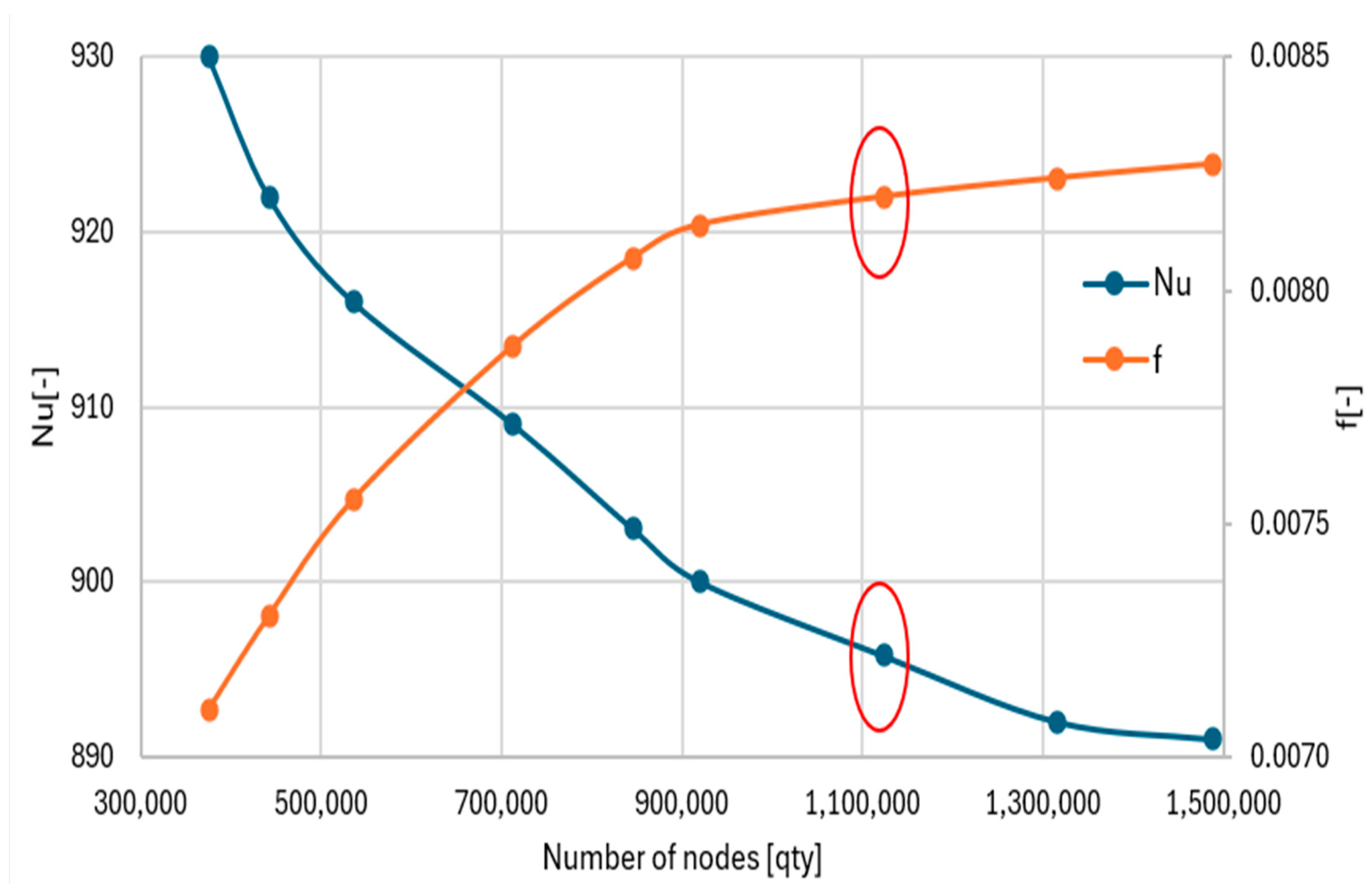
3.4. Mesh Independence Test

A series of test calculations were performed for the prepared geometry in order to select the most optimal computational grid, taking into account both the accuracy of the results and their density. Sample calculations were performed for the highest velocities in the range studied, changing the overall density of the grid as well as the size of the elements in the boundary layer. Two parameters were chosen as a comparison criterion: the Nusselt number and the friction factor. Nine variants of the mesh were tested with the following numbers of nodes, as shown in

Table 2. Number of mesh nodes used in the independence test.

Mesh	A	B	C	D	E	F	G	H	I
Number of nodes	3.14 × 105	3.66 × 105	4.77 × 105	6.06 × 105	8.29 × 105	9.91 × 105	1.12 × 106	1.32 × 106	1.49 × 106
Average y+	6.81	5.73	4.69	3.34	2.27	1.90	1.52	1.26	1.09

. The test was performed for the previously adopted boundary conditions for the highest velocities in the range studied. The mesh can be considered as independent if a further increase in the number of nodes causes a change in the monitored parameters of no more than 1–2%. The graph shown in Figure 4 shows that as the number of nodes of the grid increases, the Nusselt number decreases and the friction factor increases. The variability of these parameters is greatest until the mesh density reaches ca. 1.1 × 10⁵, and above this number of nodes, the monitored parameters practically do not change. Therefore, among the meshes studied, the “G” mesh with the number of nodes of 1.12 × 10⁶ was chosen, since for denser meshes the change in parameters averages about 0.5%.

4. Results

4.1. Data Processing

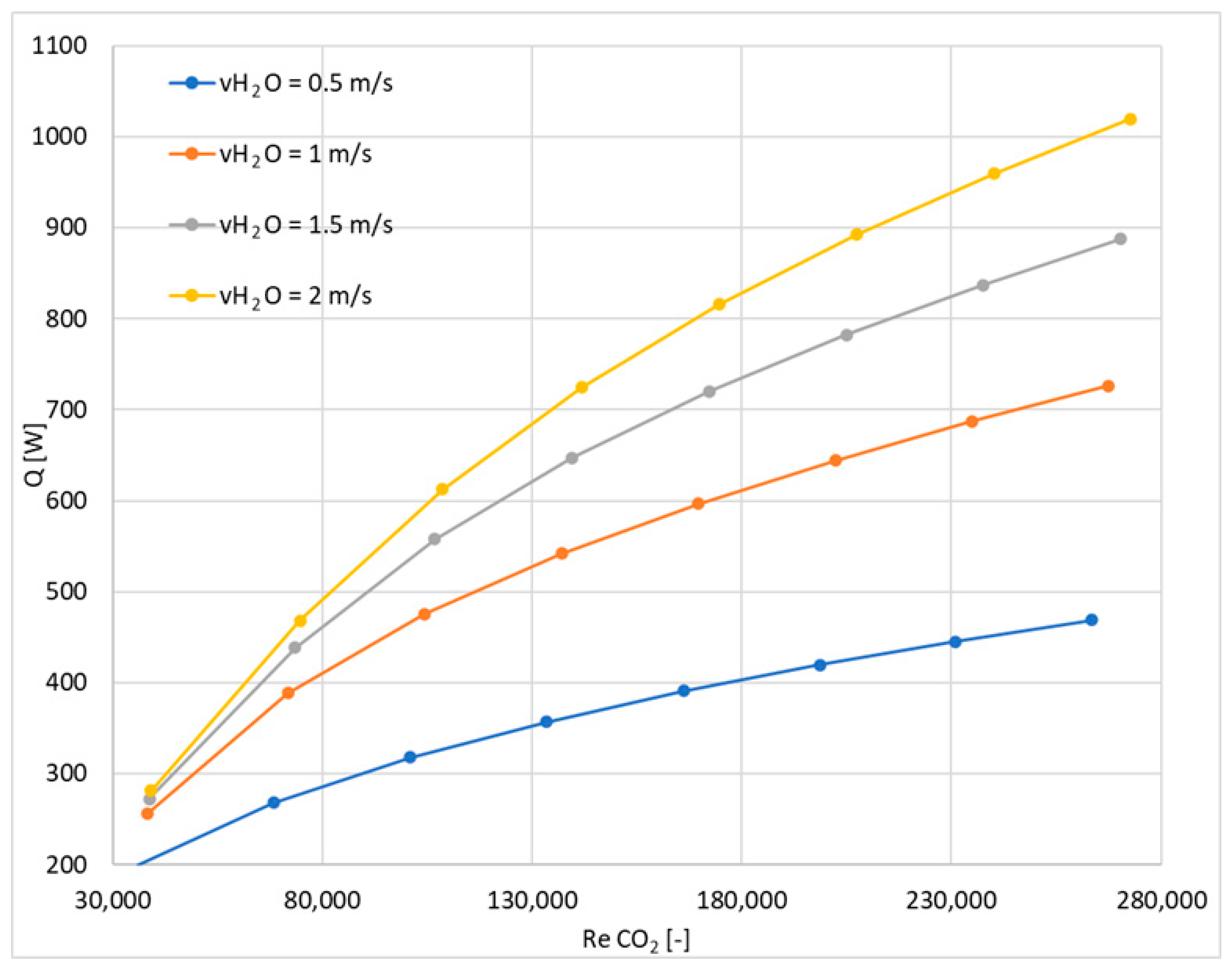
The following relationships were used to determine the thermal-fluid characteristics of the condenser. The temperature variation in thermophysical parameters of fluids was taken into account in all calculated quantities.

The friction factor was determined from the Darcy–Weisbach Equation (1):

$$ft={\displaystyle \frac{2\times D\times \mathsf{\Delta }p}{\rho \times u_{av}^2\times L}}$$

(1)

The Reynolds number was calculated according to Equation (2):

$$Re={\displaystyle \frac{\rho \times u_{av}\times D}{\mu }}$$

(2)

Nusselt number for both sCO₂ and water was calculated from Equation (3):

$$Nu={\displaystyle \frac{h\times \delta }{\lambda }}$$

(3)

where δ is the characteristic dimension: for a pipe, it is its diameter δ = D, while for an annular section, it is δ = Dz − D, i.e., the difference in diameters of the pipes.

Heat transfer coefficient h is determined from Equation (4):

$$h={\displaystyle \frac{q}{T_w-T_b}}$$

(4)

where T_b is the bulk temperature calculated as an average temperature of the fluid.

The heat transfer intensity between the two fluids in the exchanger characterizes the overall heat transfer coefficient U, which is determined by the LMTD method, when the inlet and outlet temperatures of the fluids are known, Equation (5):

$$U={\displaystyle \frac{\dot{Q}}{A_s\times {∆T}_{LMTD}}}$$

(5)

$$\dot{Q}={\displaystyle \frac{q}{A}}$$

$${∆T}_{LMTD}={\displaystyle \frac{(T_{h,in}-T_{c,out})-(T_{h,out}-T_{c,in})}{\mathrm{l}\mathrm{n}\left(\frac{T_{h,in}-T_{c,out}}{T_{h,out}-T_{c,in}}\right)}}$$

Prandtl number was determined according to Equation (6):

$$Pr={\displaystyle \frac{C_p\times \mu }{\lambda }}$$

(6)

4.2. Heat Transfer

4.2.1. Nusselt Number Empirical Correlations

An important part of the analysis of numerical studies is the verification of the obtained results with experimental correlations presented by other researchers in their works [3,18]. Several empirical correlations of the Nusselt number, both general and dedicated to supercritical CO₂, were selected.

Equation (7) shows the Dittus–Boelter correlation [24], one of the oldest and most widely used formulas for flow in a smooth circular pipe:

$$\begin{array}{c}Nu=0.023\times {Re}^{0.8}\times {Pr}^n\\ n=0.3-forcooling\\ n=0.4-forheating\end{array}$$

(7)

Equation (8) shows Gnielinski correlations [25]. It is also a universal formula for calculating the Nusselt number, especially in the transient and turbulent range, since it takes into account the friction factor f determined from the Filonenko equation:

$$\begin{gathered} Nu={\displaystyle \frac{\left(\frac{f}{8}\right)\times \left({Re}_w-1000\right)\times {Pr}_w}{1.07+12.7\times \sqrt{\frac{f}{8}}\times \left({Pr}_w^{\frac{2}{3}}-1\right)}} \\ f={\left(0.79\times ln{(Re}_b)-1.64\right)}^{-2} \end{gathered}$$

(8)

Equation (9) shows the correlation presented in the study described in Pitla et al. [26] performed to determine the correlation of Nusselt numbers during supercritical CO₂ cooling in a circular channel. It uses the arithmetic average of the Nusselt number in the temperature of the boundary layer and in the bulk temperature, determined from the Gnielinski equation [25] and the average heat conductivity in the temperature boundary layer and in the bulk temperature:

$$Nu=\left({\displaystyle \frac{{Nu}_w+{Nu}_w}{2}}\right)\times {\displaystyle \frac{{\lambda }_w}{{\lambda }_b}}$$

(9)

Equation (10) is the correlation of Ding and Li [27], which describes the average Nusselt number of supercritical CO₂ during cooling. The correlation is applicable for flows with Reynolds numbers in the range of 1.2 × 10⁵–4.97 × 10⁵ and Prandtl numbers in the range of 1.8–13.16, which translates into applications in high-turbulent flows:

$${Nu}_b=0.028\times {Re}^{0.837}\times {Pr}^{0.078}$$

(10)

Equation (11) describes the Saltanov correlation [28], which, in addition to Reynolds and Prandtl numbers, uses the ratio of the average density in the boundary layer to the average density in the bulk:

$$Nu=0.0164\ast {Re}_b^{0.823}\times {Pr}_b^{0.195}\times {\left({\displaystyle \frac{{\rho }_w}{{\rho }_b}}\right)}^{0.374}$$

(11)

Equation (12) represents the Huai and Koyama [29] correlation, dedicated to microchannels, which uses standard criterion numbers, density, and average heat capacity and heat capacity in the boundary layer. The average heat capacity was defined as the difference in average enthalpy in the boundary layer and in the bulk divided by the difference in average temperatures in the boundary layer and in the bulk:

$$\begin{gathered} Nu=0.0183\ast {Re}_b^{0.82}\times {Pr}_b^{0.5}\times {\left({\displaystyle \frac{{\rho }_w}{{\rho }_b}}\right)}^{0.3}\times {\left({\displaystyle \frac{\overline{c_p}}{c_{p,w}}}\right)}^{0.0832} \\ \overline{c_p}={\displaystyle \frac{h_b-h_w}{T_b-T_w}} \end{gathered}$$

(12)

The last equation for the correlation of the Nusselt number (13) shows the correlation of Oh and Son [30], which was obtained based on a modification of the Dittus–Boelter equation [24], with modified power exponents and using the ratio of heat capacities in the bulk and in the boundary layer:

$$Nu=0.023\times {Re}_b^{0.7}\times {Pr}_b^{2.5}\times {\left({\displaystyle \frac{c_{p,b}}{c_{p,w}}}\right)}^{-3.5}$$

(13)

4.2.2. Thermophysical Characteristics of sCO₂ in Tube Heat Exchanger

Figure 5 shows the cooling power of sCO₂ as a function of Reynolds number for different inlet velocities of cooling water. The cooling power Q is exponentially proportional to the inlet velocities of both sCO₂ and the cooling water, and thus also to the mass flows of these fluids. The cooling power increase is the result of both an increase in sCO₂ and an increase in cooling water velocity. For a cooling water velocity of 0.5 m/s, the increase in cooling power between the highest and lowest sCO₂ velocity in the studied range is more than twice, while for a velocity of 2 m/s, it is almost four times. Simulation results indicate that the condenser under study can generate cooling power in a wide range from 100 to 1000 W, depending on the set flow parameters.

Figure 6 shows the dependence of the heat transfer coefficient sCO₂ as a function of the Reynolds number of sCO₂, for different cooling water inlet velocities. Similarly to the cooling power, the heat transfer coefficient on the sCO₂ side increases proportionally to the fluid inlet velocities. The higher the sCO₂ velocity, the more the increase in water velocity influences the heat transfer coefficient. In the 1–2 m/s sCO₂ inlet velocity range, an increase in water flow causes the heat transfer coefficient to increase by about 30%, and for velocities above 4 m/s sCO₂, an increase in water velocity causes the h coefficient to increase by about 50%. The curves presented in the graph are non-linear—initially showing a large increase, which gradually flattens out at higher Re values. This may indicate that convection efficiency is approaching its limit under the given geometric and flow conditions. vH₂O = 0.5 m/s.

Analysis of the graph presented in Figure 7 indicates that for all considered cases, a clear upward trend of the overall heat transfer coefficient U is observed with the increase in the CO₂ Reynolds number. This means that increasing the CO₂ flow rate leads to an increase in the heat exchange intensity. At the same time, a significant effect of the water flow rate is noticeable: the higher its speed, the higher U coefficient values can be obtained for a given CO₂ Reynolds number. High heat transfer efficiency, characterized by U values exceeding 4500 W/m²·K, was obtained at the highest values of the CO₂ Reynolds number and at the maximum analyzed water velocity (2 m/s). The obtained results clearly indicate that in order to increase the heat transfer efficiency in the tube-in-tube exchanger, it is beneficial to both increase the velocity and, consequently, turbulence of the medium flow on the CO₂ side, as well as to increase the water flow velocity. Analysis of Figure 8 shows that the Nusselt number increases with the increase in the CO₂ Reynolds number. However, the significant effect of water velocity on the Nusselt number value on the CO₂ side indicates the coupling of flow and thermal conditions on both sides of the exchanger. Greater water influence improves heat transfer on the CO₂ side, which can be mainly explained by the variability of thermophysical properties of sCO₂.

Figure 9 shows a comparison of the previously mentioned experimental correlations of the Nusselt number, in relation to the Nu number obtained from the simulation, for a water velocity of 2 m/s (black line without points). The black dashed lines indicate error values at the level of +/− 15%. The results show that the best fit was obtained for the correlation of Pitla et al. [26] (9), which very accurately reproduced the simulation results in the entire range of Reynolds numbers studied. For Reynolds number values up to 2 × 10⁵, the Ding and Li correlation [27] (10) also falls within the assumed error limits, showing higher values of the Nusselt number in relation to those obtained in the simulation. The Nu numbers calculated based on the remaining correlations give lower values than in the simulation and deviate from the results much more than the assumed 15%.

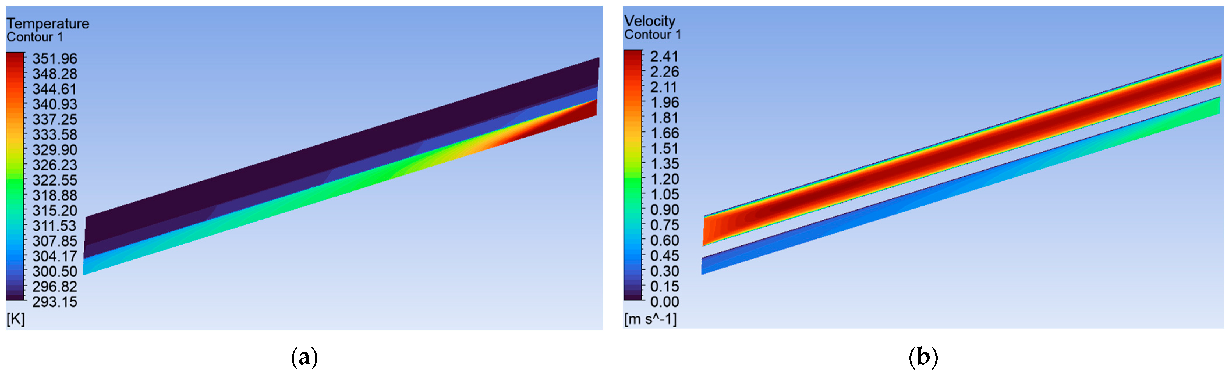
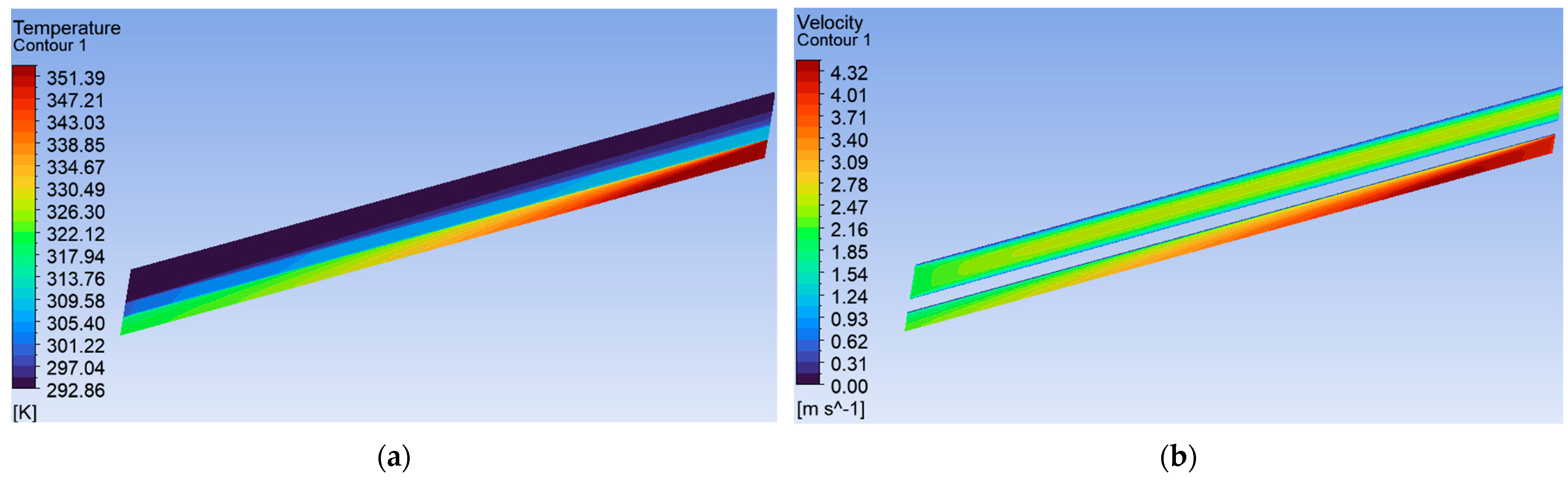
4.2.3. Temperature and Velocity Profiles

In addition to the thermal-flow characteristics, the numerical results are supplemented by the velocity and temperature field profiles in the heat exchanger, which is quite difficult to obtain from experimental studies. The results presented in Section 4.2.2. have shown that the water velocity has a significant effect on the heat transfer in the exchanger, especially to the sCO₂ side. The greater the water flow, the greater the heat transfer, and therefore the higher the heat transfer and overall heat transfer coefficients. Nusselt numbers, Reynolds numbers, and cooling power also increase, reaching up to 1 kW for the highest fluid velocities. The temperature and velocity fields, in Figure 10, Figure 11 and Figure 12, have been shown on the plane of symmetry for the water velocity of 2 m/s and for three selected CO₂ inlet velocities: 1, 4, and 8 m/s.

The analyzed heat exchanger is counterflow, with a CO₂ inlet on the right and a water inlet on the left. The above Figure 10a, Figure 11a and Figure 12a clearly show that the largest temperature difference between the CO₂ inlet and outlet is for the smallest inlet velocity of 1 m/s, and is Δt = 45.1 °C. With the increase in the CO₂ inlet velocity, this difference decreases and reaches the values: for 4 m/s, Δt = 34.4 °C, and for 8 m/s, Δt = 29.2 °C, while the mass flow rate, heat transfer coefficient, and consequently the heat flow exchanged between the fluids increase. Figure 10b, Figure 11b and Figure 12b indicate that the water velocity is constant along the entire length of the pipe, while cooling sCO₂ causes a significant decrease in velocity. It is greatest for the smallest CO₂ inlet velocity of 1m/s, where for this case, the outlet velocity decreased to 0.3 m/s—which translates into a 70% drop compared to the inlet velocity. For inlet velocities of 4 and 8 m/s the velocity drop is similar—u_out = 2.13 m/s (Δu = 47.5%) for inlet velocity 4 m/s and u_out = 4.8 m/s (Δu = 40%) for inlet velocity 8 m/s.

4.3. Friction Factor

Similarly to the Nusselt number, several friction factor correlations were selected for comparison with simulation results [31]. The friction factor was calculated from the Darcy–Weisbach Equation (1), based on the knowledge of the pressure drop, average velocity, and fluid density obtained from numerical simulations. Figure 13 shows a graph of the friction factor for CO₂ as a function of CO₂ Reynolds number, for different water velocities. The results from the graph show that for a water velocity of 0.5 m/s, the friction factor decreases with the increase in the Reynolds number of CO₂. For higher water velocities, this trend is rather opposite, i.e., with the increase in the Re number the friction factor of CO₂ slightly increases.

The general tendency is that the increase in the water velocity leads to a general decrease in flow resistance, which can be seen in other characteristics. The influence of the water velocity on the flow resistance of CO₂ is therefore very clear. This is mainly due to the change in the heat transfer intensity between the fluids and, consequently, the change in the thermal conditions of CO₂ and the associated changes in the properties of the physicochemical parameters of CO₂, such as thermal conductivity, viscosity, or density.

Several friction factor correlations were selected for comparison with the simulation results and will also be presented for the sCO₂ value at a water velocity of 2 m/s. Equation (14) describes one of the basic friction factor correlations, given by Blasius [32], which has theoretical application for a perfectly smooth pipe. In the turbulent flow in the range 2 × 10⁴ to 2 × 10⁶, the equation has the following form:

$$f={\displaystyle \frac{0.184}{{Re}^{0.2}}}$$

(14)

Equation (15) describes the Popov correlation [33] dedicated to determining the friction factor in supercritical CO₂ flow, where coefficient f_iso,b is determined from the Filonenko Equation (16) and coefficient ρ_f refers to the density at film temperature, which is the arithmetic average of the bulk and the boundary layer temperature:

$$f=f_{iso,b}\times {\left({\displaystyle \frac{{\rho }_f}{{\rho }_b}}\right)}^{0.74}$$

(15)

$$f_{iso,b}={\left(0.79\times ln{(Re}_b)-1.64\right)}^{-2}$$

(16)

Kutateladze correlation [34] is given by Equation (17):

$$f=f_{iso,b}\times {\left({\displaystyle \frac{2}{\sqrt{\frac{T_w}{T_b}}+1}}\right)}^2$$

(17)

Figure 14 shows the friction coefficients as a function of the Reynolds number of sCO₂, calculated using the mentioned correlations. The Blasius (orange line) and the Kutateladze formula (purple line) give results that are very similar to each other—the friction factor values are almost identical in the entire range of the analyzed data, and both curves show a clearly decreasing trend of the friction factor with the increase in the Reynolds number. The Popov formula (gray line) shows the highest friction factor among all correlations. Initially, it increases, reaches a maximum in the range of Re ≈ 80,000, and then slowly decreases. In general, due to the small change in its value in the entire range of the Re number, they can be assumed to be approximately constant. However, there are significant differences between the presented models, especially between Blasius (14), Kutateladze (17) and Popov (15), but each of them significantly differs from the friction factor from the numerical simulation, where the main influence on its values is the temperature variability of the physical parameters of the fluid.

5. Discussion

The numerical analyses performed allowed for a detailed characterization of heat transfer and flow of supercritical CO₂ in a tube-in-tube condenser in a wide range of operating parameters. The results showed that increasing the flow rate of both CO₂ and cooling water significantly improves the heat transfer intensity (Figure 6, Figure 7 and Figure 8). An exponential increase in cooling power was observed as a function of flow rate, which confirms the strong coupling of flow-thermal parameters on both sides of the heat exchanger (Figure 5). The heat transfer and overall heat transfer coefficients show an increasing trend with the increase in the Reynolds number, while the dynamics of this increase decrease in higher speed ranges, indicating that the limits of convective heat transfer efficiency are being approached. The highest values of the overall heat transfer coefficient U exceeded 4500 W/m²·K, which proves the high potential of the compact heat exchanger for applications in small refrigeration systems (Figure 7).

Comparison of numerical results with empirical correlations of Nusselt number (Figure 9) showed very good agreement, especially with reference to the models of Pitla et al. and Ding and Li, which confirms the correctness of the adopted calculation methodology. The analysis of the CO₂ friction factor obtained from the simulations showed a significant impact of water velocity on its value, but with respect to the correlations by Blasius (14), and those dedicated to supercritical flows, Popov (15) and Kutateladze (17), which show significant discrepancies.

The results obtained clearly indicate that by appropriate selection of flow parameters, it is possible to significantly increase the heat transfer efficiency of the heat exchanger without changes in its design. In further work, it is recommended to consider the influence of additional factors, such as modification of the exchanger geometry, introduction of flow disturbances (e.g., by using fins or special internal structures), and optimization of operating parameters in terms of minimizing pressure losses and maximizing cooling efficiency.

6. Conclusions

Based on the numerical studies presented in this paper, the most important conclusions were formulated:

• Numerical simulations confirmed that increasing the flow rate of supercritical CO₂ and cooling water significantly improves the heat transfer efficiency in the tube-in-tube condenser;
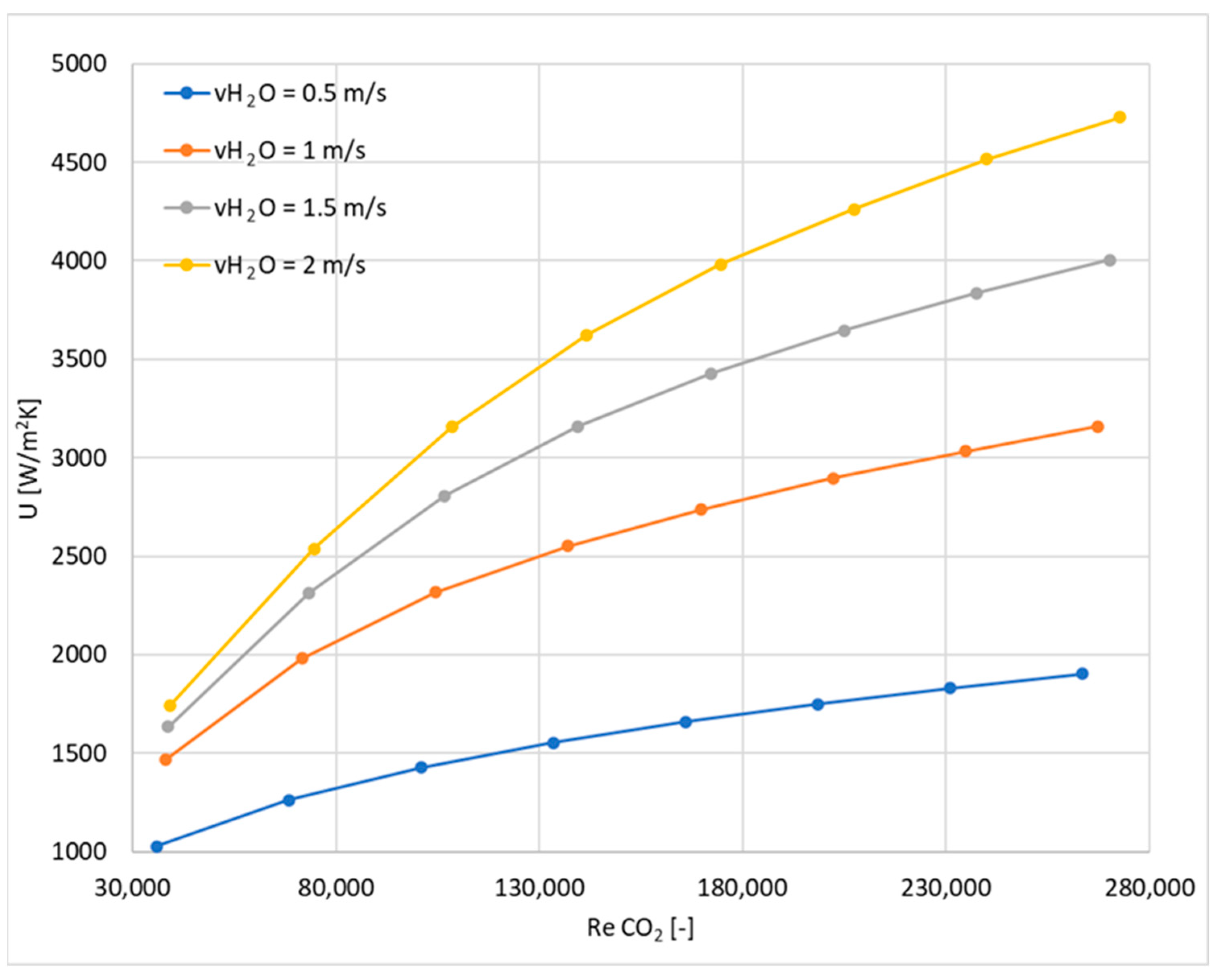
• The overall heat transfer coefficient U exceeded 4500 W/m² K at the highest analyzed flow rates, which confirms the high efficiency of the system;
• The Nusselt number and heat transfer coefficient increase nonlinearly with the increase in the Reynolds number and flow velocity;
• Friction factor tests showed that increasing water velocity leads to a decrease in CO₂ flow resistance for the same Reynolds number;
• The results of the work indicate that optimizing the difference in CO₂ and water flow velocities is crucial for obtaining high cooling efficiency;
• The developed methodology and results can be used to design compact, ecological cooling systems using CO₂.

References

1. Cavallini, A.; Zilio, C. Carbon dioxide as a natural refrigerant. Int. J. Low-Carbon Tech. 2007, 2, 225–249. [Google Scholar] [CrossRef]
2. Bansal, P. A review—Status of CO2 as a low temperature refrigerant: Fundamentals and R&D opportunities. Appl. Therm. Eng. 2012, 41, 18–29. [Google Scholar]
3. Thiwaan Rao, N.; Oumer, A.N.; Jamaludin, U.K. State-of-the-art on flow and heat transfer characteristics of supercritical CO2 in various channels. J. Supercrit. Fluids 2016, 116, 132–147. [Google Scholar]
4. Alsouda, F.; Bennett, N.S.; Saha, S.C.; Islam, M.S. A Novel Direct-Expansion Radiant Floor System Utilizing Water (R-718) for Cooling and Heating. Energies 2024, 17, 4520. [Google Scholar] [CrossRef]
5. Shah, M.M. Prediction of Heat Transfer during Condensation of Ammonia Inside Tubes and Annuli. Energies 2024, 17, 4869. [Google Scholar] [CrossRef]
6. Wang, Y.-Z.; Fan, Y.-W.; Li, X.-L.; Yang, J.-G.; Zhang, X.-R. Experimental Validation of a Novel CO2 Refrigeration System for Cold Storage: Achieving Energy Efficiency and Carbon Emission Reductions. Energies 2025, 18, 1129. [Google Scholar] [CrossRef]
7. Carella, A.; D’Orazio, A. A Systematic Review on Heat Transfer and Pressure Drop Correlations for Natural Refrigerants. Energies 2024, 17, 1478. [Google Scholar] [CrossRef]
8. Wu, D.; Wei, M.; Tian, R.; Zheng, S.; He, J. A Review of Flow and Heat Transfer Characteristics of Supercritical Carbon Dioxide under Cooling Conditions in Energy and Power Systems. Energies 2022, 15, 8785. [Google Scholar] [CrossRef]
9. Liao, S.M.; Zhao, T.S. Measurements of Heat Transfer Coefficients from Supercritical Carbon Dioxide Flowing in Horizontal Mini/Micro Channels. J. Heat Transf. 2002, 124, 413–420. [Google Scholar] [CrossRef]
10. Dang, C.; Hihara, E. In–tube cooling heat transfer of supercritical carbon dioxide. Part 1. Experimental measurement. Int. J. Refrig. 2004, 27, 736–747. [Google Scholar] [CrossRef]
11. Zhang, G.W.; Hu, P.; Chen, L.X.; Chen, L.X.; Liu, M.H. Experimental and simulation investigation on heat transfer characteristics of in–tube supercritical CO2 cooling flow. Appl. Therm. Eng. 2018, 143, 1101–1113. [Google Scholar] [CrossRef]
12. Lei, Y.; Xu, B.; Chen, Z. Experimental investigation on cooling heat transfer and buoyancy effect of supercritical carbon dioxide in horizontal and vertical micro–channels. Int. J. Heat Mass Transf. 2021, 181, 121792. [Google Scholar] [CrossRef]
13. Wahl, A.; Mertz, R.; Laurien, E.; Starflinger, J. Heat transfer correlation for sCO2 cooling in a 2 mm tube. J. Supercrit. Fluids 2021, 173, 105221. [Google Scholar] [CrossRef]
14. Tu, Y.; Zeng, Y. Flow and heat transfer characteristics study of supercritical CO2 in horizontal semicircular channel for cooling process. Case Stud. Therm. Eng. 2020, 21, 100691. [Google Scholar] [CrossRef]
15. Du, Z.; Lin, W.; Gu, A. Numerical investigation of cooling heat transfer to supercritical CO2 in a horizontal circular tube. J. Supercrit. Fluids 2010, 55, 116–121. [Google Scholar] [CrossRef]
16. Wang, X.; Xiang, M.; Huo, H.; Liu, Q. Numerical study on nonuniform heat transfer of supercritical pressure carbon dioxide during cooling in horizontal circular tube. Appl. Therm. Eng. 2018, 141, 775–787. [Google Scholar] [CrossRef]
17. Xiang, M.; Guo, J.; Huai, X.; Cui, X. Thermal analysis of supercritical pressure CO2 in horizontal tube under cooling condition. Int. J. Supercrit. Fluids 2017, 130, 389–398. [Google Scholar] [CrossRef]
18. Cabeza, L.F.; de Garcia, A.; Inés Fernández, A.; Farid, M.M. Supercritical CO2 as heat transfer fluid: A review. Appl. Therm. Eng. 2017, 125, 799–810. [Google Scholar] [CrossRef]
19. Jasiński, P.B.; Górecki, G.; Cebulski, Z. Evaluation of the Efficiency of Heat Exchanger Channels with Different Flow Turbulence Methods Using the Entropy Generation Minimization Criterion. Energies 2025, 18, 132. [Google Scholar] [CrossRef]
20. Jasiński, P.B. Numerical Investigation of Thermo-Flow Characteristics of Tubes with Transverse Micro-Fins. Energies 2024, 17, 714. [Google Scholar] [CrossRef]
21. Zhu, Q.; Su, R.; Xia, H. Numerical simulation study of thermal and hydraulic characteristics of laminar flow in microchannel heat sink with water droplet cavities and different rib columns. Int. J. Therm. Sci. 2022, 172 Pt B, 107319. [Google Scholar] [CrossRef]
22. ANSYS. CFX-Solver Theory Guide; ANSYS, Inc.: Canonsburg, PA, USA, 2021. [Google Scholar]
23. ANSYS. CFX-Pre User’s Guide; ANSYS, Inc.: Canonsburg, PA, USA, 2021. [Google Scholar]
24. Dittus, F.W.; Boelter, L.M.K. Heat transfer in automobile radiators of the tubular type. Univ. Calif. Publ. Eng. 1930, 2, 443–461. [Google Scholar] [CrossRef]
25. Gnielinski, V. New equation for heat and mass transfer in turbulent pipe and channel flow. Int. Chem. Eng. 1976, 16, 359–368. [Google Scholar]
26. Pitla, S.S.; Groll, E.A.; Ramadhyani, S. New correlation to predict the heat transfer coefficient during in-tube cooling of turbulent supercritical CO2. Int. J. Refrig. 2002, 25, 887–895. [Google Scholar] [CrossRef]
27. Ding, T.; Li, Z. Research on convection heat transfer character of super critical carbon dioxide flows inside horizontal tube. Int. J. Heat Mass Transf. 2016, 92, 665–674. [Google Scholar] [CrossRef]
28. Saltanov, E.; Pioro, I.; Mann, D.; Gupta, S.; Mokry, S.; Harvel, G. Study on specifics of forced-convective heat transfer in supercritical carbon dioxide. J. Nucl. Eng. Radiat. Sci. 2015, 1, 1–8. [Google Scholar] [CrossRef]
29. Huai, X.; Koyama, S. Heat transfer characteristics of supercritical CO2 flow in small-channeled structures. Exp. Heat Transf. 2007, 20, 19–33. [Google Scholar] [CrossRef]
30. Oh, H.K.; Son, C.H. New correlation to predict the heat transfer coefficient in-tube cooling of supercritical CO2 in horizontal macro-tubes. Exp. Therm. Fluid Sci. 2010, 34, 1230–1241. [Google Scholar] [CrossRef]
31. Fang, X.; Xu, Y.; Su, X.; Shi, R. Pressure drop and friction factor correlations of supercritical flow. Nucl. Eng. Des. 2012, 242, 323–330. [Google Scholar] [CrossRef]
32. Vijayan, P.K.; Nayak, A.K.; Kumar, N. Chapter 3 Governing differential equations for natural circulation systems. In Single-Phase, Two-Phase and Supercritical Natural Circulation Systems; Woodhead Publishing: Cambridge, UK, 2019; pp. 69–118. ISBN 978-0-08-102486-7. [Google Scholar]
33. Popov, V.N. Theoretical calculation of heat transfer and friction resistance for supercritical carbon dioxide. In Proceedings of the Second All-Soviet Union Conference on Heat and Mass Transfer, Minsk, Belarus, 5–9 May 1964; Gazley, C., Jr., Hartnett, J.P., Ecker, E.R.C., Eds.; Published as Rand Report R-451-PR 1. 1967; pp. 46–56. [Google Scholar]
34. Kutateladze, S.S. The Element of Heat Exchange; Mashgiz: Moscow-Leningrad, Russia, 1962. [Google Scholar]
Figure 1. Thermophysical properties of CO2 as a function of temperature at supercritical pressures: density (a), dynamic viscosity (b), heat capacity at constant pressure (c), and thermal conductivity (d).
Energies 18 02992 g001
Figure 2. Radial cross-section and isometric view of the analyzed geometry.
Energies 18 02992 g002
Figure 3. Analyzed geometry with boundary conditions.
Energies 18 02992 g003
Figure 4. Mesh independence test results.
Energies 18 02992 g004
Figure 5. Cooling power Q as a function of sCO2 Reynolds number.
Energies 18 02992 g005
Figure 6. Heat transfer coefficient h of sCO2 as a function of sCO2 Reynolds number.
Energies 18 02992 g006
Figure 7. Heat transfer coefficient U of sCO2 as a function of sCO2 Reynolds number.
Energies 18 02992 g007
Figure 8. sCO2 Nusselt number as a function of sCO2 Reynolds number.
Energies 18 02992 g008
Figure 9. Correlations of sCO2 Nusselt number as a function of CO2 Reynolds number.
Energies 18 02992 g009
Figure 10. Temperature field (a), velocity field (b) for inlet velocity CO2 = 1 m/s.
Energies 18 02992 g010
Figure 11. Temperature field (a), velocity field (b) for inlet velocity CO2 = 4 m/s.
Energies 18 02992 g011
Figure 12. Temperature field (a), velocity field (b) for inlet velocity CO2 = 8 m/s.
Energies 18 02992 g012
Figure 13. Friction factor of CO2 obtained from numerical calculations as a function of the Reynolds number of CO2, for different water velocities.
Energies 18 02992 g013
Figure 14. Illustration of the friction factor based on the correlations described by Equations (14), (15), and (17) compared with the friction factor determined from the simulation as a function of the Reynolds number of CO2, at a water inlet velocity of 2 m/s.
Energies 18 02992 g014