Article

Robust Wide-Speed-Range Control of IPMSM with Multi-Axis Coordinated Extended State Observer for Dynamic Performance Enhancement

1
School of Electrical Engineering and Automation, Harbin Institute of Technology, Harbin 150001, China
2
School of Mechatronics Engineering, Harbin Institute of Technology, Harbin 150001, China
*
Author to whom correspondence should be addressed.
Energies 2025, 18(11), 2938; https://doi.org/10.3390/en18112938
Submission received: 29 April 2025 / Revised: 11 May 2025 / Accepted: 30 May 2025 / Published: 3 June 2025
(This article belongs to the Section F: Electrical Engineering)

Abstract

Wide-speed regulation control strategies for Interior Permanent Magnet Synchronous Motors (IPMSMs) are widely applied in industrial fields. However, traditional algorithms are prone to being affected by motor parameter mismatches, sensor sampling errors, and other disturbances under complex operating conditions, leading to insufficient robustness. In order to enhance dynamic performance while simultaneously ensuring robustness, we analyzed the limitations of traditional control strategies and, based on this, proposed an improved control framework. A Multi-Axis Coordinated Extended State Observer(MCESO)-based robust control framework was developed for full-speed domain operation, which enhances disturbance rejection capability against parameter uncertainties and abrupt load changes through hierarchical disturbance estimation. Subsequently, the effectiveness and stability of the proposed method were verified through theoretical analysis and simulation studies. Compared with traditional control strategies, this method can effectively observe and compensate for a series of complex issues such as nonlinear disturbances during operation without requiring additional hardware support. Finally, extensive experimental tests were carried out on a 500 W IPMSM dual-motor drive platform. The experimental results demonstrated that, even under harsh operating conditions, the proposed scheme can effectively suppress torque ripple and significantly reduce current harmonics.

1. Introduction

Interior Permanent Magnet Synchronous Motors (IPMSMs) have found widespread applications in electric vehicles, AI systems, and home appliances owing to their high efficiency, power density, and control accuracy [1,2,3,4]. However, as application requirements increasingly demand wider speed regulation ranges for drive systems, achieving full-speed-range high-precision control of IPMSMs has become a key technical challenge for enhancing system performance [5]. For IPMSMs, although Maximum Torque Per Ampere (MTPA) and flux-weakening control enhance efficiency, their traditional implementation relies on offline lookup table methods [6,7]. To address this, Refs. [8,9] introduced a geometric iteration algorithm to improve computational efficiency. Traditional full-speed-range control algorithms exhibit slow dynamic responses and insufficient robustness under parameter perturbations and inverter nonlinear coupling conditions [10]. This highlights the critical need for developing robust, dynamic-performance-enhanced control strategies across entire speed ranges.
Dynamic performance typically comprises two critical metrics, disturbance rejection capability and response speed. Traditional PI controllers exhibit limited dynamic regulation capability under multi-disturbance operating conditions. Their fixed-gain characteristics fail to accommodate the nonlinear control requirements of multivariable coupled systems [11]. To address this, Han’s research team integrated classical PI negative feedback mechanisms with modern state observer methods, proposing Nonlinear Active Disturbance Rejection Control (NLADRC) [12]. This strategy employs an extended state observer (ESO) to identify internal and external disturbances in real time, coupled with nonlinear feedback for dynamic compensation, thereby enhancing both stability and response speed under time-varying disturbances while maintaining control precision. Ref. [13] innovatively restructured the core state observer architecture of NLADRC by decoupling system disturbances into low-frequency and high-frequency components. Through a two-stage cascaded ESO structure for frequency-selective disturbance compensation, combined with an enhanced nonlinear state error feedback mechanism, the dynamic disturbance rejection capability of continuous-wave pulse generators was significantly improved. Furthermore, this improved ESO framework has been extended to sensorless control of permanent magnet synchronous motors [14], where its phase delay suppression effectively reduces rotor position estimation errors, substantially increasing the disturbance rejection bandwidth in sensorless operation modes.
To enhance dynamic response performance, conventional PI controllers typically employ control bandwidth expansion and adaptive gain optimization strategies [15]. With the continuous advancements in chip computational power, Model Predictive Control (MPC) has been widely implemented in motor control systems. Ref. [16] implemented a Model Predictive Speed Control (MPSP) algorithm to replace traditional PI regulators, achieving enhanced dynamic response speed in the speed loop of dual three-phase motor drive systems. Additionally, Direct Torque Control (DTC), as a typical method for PMSM drives, directly regulates stator flux vectors and electromagnetic torque. While widely adopted in industrial applications due to its simple architecture, fast dynamics, and excellent robustness, DTC suffers from significant torque ripples and switching frequency fluctuations caused by inherent discrete vector modulation strategies [17,18,19]. Furthermore, for current loop control, Model Predictive Current Control (MPCC) emerges as a high-performance strategy. This method leverages finite control set predictive frameworks or deadbeat control principles to optimize multi-objective cost functions (e.g., current tracking errors, switching losses), enabling rapid and precise stator current regulation. MPCC demonstrates superior dynamic response and harmonic suppression capabilities [20,21,22,23,24,25].
Robustness is a key measure of control system performance, requiring both handling parameter changes and resisting disturbances. MPCC heavily relies on accurate motor models and parameters [26]. However, the changing parameters in IPMSMs reduce the accuracy of model-based closed-loop control and can even cause instability risks [27,28]. A predictive current error compensation strategy developed in [10] enhanced system robustness but neglected sampling bias errors, which are also critical factors limiting robustness due to environmental interference [29,30]. A method in [31] integrated controllable error injection with model-reference adaptive observers to suppress high-frequency disturbances and mitigate parasitic effects. Research presented in [32] implemented closed-loop compensation for sampling bias errors via ESO, yet demonstrated limited response speed due to constraints in conventional FOC architectures.
To address combined disturbances from motor parameter mismatch and current sampling errors, this paper proposes a Multi-axis Coordinated ESO(MCESO) control framework. By integrating disturbance observation and dynamic compensation, it achieves high dynamic response and robust control across full-speed ranges. The innovative aspects of this strategy are summarized as follows: Firstly, a novel MCESO full-speed-range control architecture is proposed, which simultaneously improves traditional nonlinear functions to ensure dynamic responses while reducing operational current harmonics. Secondly, based on bandwidth configuration methodology, the parameter mismatch coupling problem under coordinated observers in multi-disturbance environments is analyzed, achieving holistic enhancement of system robustness.
The remaining paper organization is structured as follows: Section 2 provides an independent analysis of the ESO compensation algorithm for current sampling bias errors. Section 3 focuses on the dq-axis ESO disturbance compensation algorithm, introducing the novel MCESO structure. Section 4 examines parameter mismatch coupling issues in multi-disturbance environments under coordinated observers and proposes solutions. Section 5 validates the control strategy through closed-loop experiments on a hardware platform. Section 6 concludes the paper.

2. Current Bias Compensation Analysis

2.1. Mathematical Model of IPMSM

The voltage model of IPMSM in the three-phase natural coordinate system is expressed as follows:
u 3 s = R s i 3 s + p L s i 3 s + e 3 s
Through Clarke transformation, the voltage model in the alpha-beta coordinate system is obtained as follows:
u α u β = R s + p L α p L α β p L α β R s + p L β i α i β + ω e ψ f sin θ e + cos θ e
To simplify the inductance terms in the equations, the model is derived using the inverse Park transformation as follows:
u α u β = R s + p L q 0 0 R s + p L q i α i β + [ ( L d L q ) ω e i d + ω e ψ f ] sin θ e + cos θ e
After applying the Park transformation, the voltage model in the dq-axis coordinate system is obtained as follows:
u d u q = R s + p L d ω e L q ω e L d R s + p L q i d i q + ω e ψ f 0 1

2.2. Current Sampling Bias Error Impact Analysis

Current sensors exhibit zero drift issues, typically manifesting as bias errors, which compromise control performance. Given that the time-varying rate of this sampling error is significantly lower than the system operating frequency, it can be approximated as a constant within individual control cycles, thereby deriving the three-phase current expression:
i a m = i a a c t + i a o f f i b m = i b a c t + i b o f f i c m = 0 i a m i b m i α m = i α a c t + i a o f f i β m = i β a c t + i β o f f i β o f f = 3 3 ( i a o f f + 2 i β o f f ) i d m = i d a c t + A o f f sin ( ω e t + φ ) i q m = i q a c t + A o f f cos ( ω e t + φ ) A o f f = i a o f f 2 + i β o f f 2 tan φ = 3 i a o f f / ( i a o f f + 2 i b o f f )
Equation (5) demonstrates that bias errors introduce first-order harmonic components in dq-axis currents. The corresponding frequency coincides with the operating frequency. For IPMSM, the total current substitution into the torque equation (see Equation (6)) reveals the following:
T e m = T e + T e o f f T e = 1.5 n p [ i d i q ( L d L q ) + ψ f i q ] T e o f f = 1.5 n p { [ A o f f cos ( ω e t + φ ) i d + A o f f sin ( ω e t + φ ) i q + A o f f 2 cos ( ω e t + φ ) sin ( ω e t + φ ) ]                           × ( L d L q ) + ψ f A o f f cos ( ω e t + φ ) }

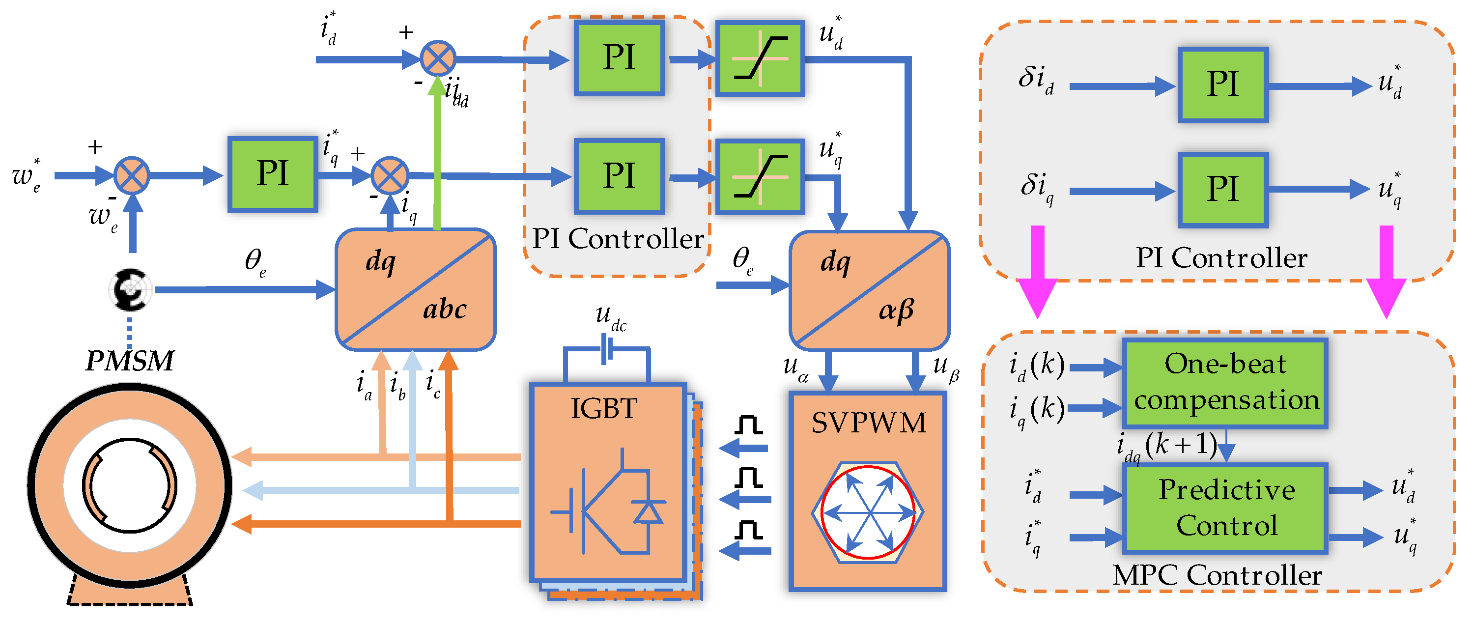
2.3. Analysis of ESO-Based Current Bias Error Algorithm

Conventional current error compensation [33] employs a PI observer to estimate error currents in the alpha-beta coordinate system, with its implementation structure depicted in Figure 1a. Because of i a o f f = i α o f f , substituting the current error equations of the alpha-beta frame into the corresponding voltage model and neglecting their first-order derivatives based on the established slowly varying disturbance characteristics, the actual current can be expressed as follows:
d i α m d t = R s L s i α m + 1 L s ω e ψ f sin θ e + 1 L s u α + R s L s i α o f f d i β m d t = R s L s i β m 1 L s ω e ψ f cos θ e + 1 L s u β + R s L s i β o f f
Assuming negligible parameter mismatches and accurate voltage measurements, the estimated current model is derived as follows:
d i ^ α m d t = R s L s i ^ α m + 1 L s ω e ψ f sin θ e + 1 L s u α + R s L s i ^ α o f f d i ^ β m d t = R s L s i ^ β m 1 L s ω e ψ f cos θ e + 1 L s u β + R s L s i ^ β o f f
Taking the alpha-axis as an example, by subtracting Equation (8) from Equation (7) and incorporating the PI-based compensation structure, Equation (9) is derived:
e α = i α m i ^ α m d e α d t = R s L s e + R s L s ( i α o f f i ^ α o f f ) e = R s i ^ α o f f s K p s + K i i ^ α o f f = K p s + K i L s s 2 + ( K p s + R s ) s + K i i α o f f
Utilizing the bandwidth configuration methodology, K p equals L s ω c and K i equals R s w c . Ref. [32] also derived the transfer function of i ^ α o f f under parameter perturbations as follows:
i ^ α o f f = w c s + w c [ R s i α o f f + δ u α δ E α + ( s δ L s + δ R s ) ( R s s L s + R s i α o f f + i α m ) ]
Theoretical analysis demonstrates that the dynamic disturbance rejection capability of this robust control strategy is inherently constrained by the limited high-frequency noise suppression performance of the first-order low-pass filter.
To address the aforementioned limitations, the ESO from the NADRC core framework was adopted to replace the PI observer. Following the same analytical approach with the alpha-axis as the exemplar, the derived error equation is given in Equation (11). Detailed derivations are provided in Appendix A.
d i α m d t d i ^ α m d t = R s L q ( i α m i ^ α m ) β 1 ( i α m i ^ α m ) + ( z α z ^ α ) d z α d t d z ^ α d t = β 2 ( i α m i ^ α m ) + d z α d t
This observer structure is illustrated in Figure 1b. Similarly, based on the bandwidth configuration method ( β 1 = 2 ω c , β 2 = ω c 2 ), the transfer function of i ^ α o f f under parameter perturbations is derived as follows:
i ^ α o f f = w c 2 s 2 + 2 w c s + w c 2 1 R s ( δ u α + δ E α + s δ L q i α m + δ R s i α m + R s i α o f f )
It is obvious that Equation (12) reveals a second-order low-pass filtering relationship between estimated current errors and actual measurement errors. Compared to Equation (10), the ESO architecture demonstrates closer approximation to ideal filter characteristics with superior frequency-domain selectivity. Section 4 will perform multifactor analysis by integrating this with the fast-response current algorithm.

3. DPCC-Based Fast-Response Robust Current Control

3.1. Current Predictive Control Based on Deadbeat Principle

The dynamic response speed of IPMSMs across their entire operating speed range is mainly limited by the bandwidth of the current control loop. Whereas conventional PI controllers exhibit limited dynamic performance and struggle with cross-coupling effects, Model Predictive Control (MPC) leverages discrete-time system models to predict future states. Through deadbeat control principles, MPC directly computes optimal voltage vectors, achieving current tracking within two control cycles under ideal conditions with inherent high-bandwidth characteristics. Furthermore, MPC demonstrates superior decoupling capability and effective multi-constraint handling.
A block diagram of conventional Deadbeat Predictive Current Control (DPCC) is illustrated in Figure 2. Considering the inherent current sampling latency and voltage application time delay in digital control systems, one-step delay compensation is implemented after essential sampling noise filtering:
i d ( k + 1 ) = ( 1 T s R s L d ) i d ( k ) + w e ( k ) T s L q L d i q ( k ) + T s u d ( k ) L d i q ( k + 1 ) = ( 1 T s R s L q ) i q ( k ) w e ( k ) T s L d i d ( k ) + ψ f L q + T s u q ( k ) L q
Subsequently, the optimal voltage output vector is derived based on the deadbeat control principle:
u d r e f = R s i d ( k + 1 ) + L d ( i d ( k + 2 ) i d ( k + 1 ) ) / T s w e ( k ) L q i q ( k + 1 ) i d ( k + 2 ) = i d r e f u q r e f = R s i q ( k + 1 ) + L d ( i q ( k + 2 ) i q ( k + 1 ) ) / T s w e ( k ) ( L d i d ( k + 1 ) + ψ f ) i q ( k + 2 ) = i q r e f

3.2. Parameter Mismatch Analysis and Robust Control Strategy

DPCC demonstrates superior dynamic performance but exhibits high sensitivity to precise motor parameters. Therefore, the integration of disturbance compensation mechanisms becomes imperative. The one-step compensation formula for current control under parameter mismatch is given in Equation (15).
i d a c t ( k + 1 ) = ( 1 ( R s + Δ R s ) L d + Δ L d T s ) i d ( k ) + T s L d + Δ L d u d ( k ) + ω e ( L q + Δ L q ) T s L d + Δ L d i q ( k ) i q a c t ( k + 1 ) = ( 1 ( R s + Δ R s ) L d + Δ L d T s ) i q ( k ) + T s L q + Δ L q u q ( k ) ω e T s [ ( L d + Δ L d ) i d ( k ) + ψ f ] L q + Δ L q
Following the deadbeat control principle, the conventional optimal voltage vector can be derived as follows:
u d a c t ( k ) = L d T s ( i d r e f i d ( k + 1 ) ) + R s i d ( k + 1 ) w e ( k ) L q i q ( k + 1 ) Nominal   Model   Term                         + Δ L d T s [ i d r e f i d ( k + 1 ) ] L d + Δ L d T s E r ( i d ) + Δ R s i d ( k + 1 ) + R s E r ( i d ) Resistance - Inductance   Mismatch   Term                         w e ( k ) Δ L q i q ( k + 1 ) w e ( k ) L q E r ( i q ) w e ( k ) Δ L q E r ( i q ) Dynamic   Cross - Coupling   Term + u n o i s e
u q a c t ( k ) = L q T s ( i q r e f i q ( k + 1 ) ) + R s i q ( k + 1 ) + w e ( k ) [ L d i d ( k + 1 ) + ψ f ] Nominal   Model   Term                         + Δ L d T s [ i q r e f i q ( k + 1 ) ] L q + Δ L q T s E r ( i q ) + Δ R s i q ( k + 1 ) + R s E r ( i q ) Resistance - Inductance   Mismatch   Term                         + w e ( k ) Δ L d i d ( k + 1 ) + w e ( k ) L d E r ( i d ) + w e ( k ) Δ L d E r ( i d ) Dynamic   Cross - Coupling   Term + u n o i s e
Equations (16) and (17) reveal that the optimal voltage vector contains complex components that cannot be effectively addressed by analytical compensation methods. Therefore, an ESO is constructed to estimate the lumped disturbances:
i d e s t ( k + 1 ) = i d e s t ( k ) R s L d T s i d ( k ) + ω e ( k ) L q L d T s i q ( k ) + T s L d u d ( k ) + T s β 1 e d + T s L d u d e s t ( k ) i q e s t ( k + 1 ) = i q e s t ( k ) R s L q T s i q ( k ) ω e ( k ) T s [ L d L q i d ( k ) + ψ f L q ] + T s L q u q ( k ) + T s β 1 e q + T s L q u q e s t ( k )
u d e s t ( k + 1 ) = u d e s t ( k ) + T s L d β 2 e d u q e s t ( k + 1 ) = u q e s t ( k ) + T s L q β 2 e q u d p = R s i d e s t ( k + 1 ) + L d ( i d r e f i d e s t ( k + 1 ) ) / T s w e ( k ) L q i q e s t ( k + 1 ) u d r e f = u d p u d e s t u q p = R s i q e s t ( k + 1 ) + L d ( i q r e f i q e s t ( k + 1 ) ) / T s w e ( k ) ( L d i d e s t ( k + 1 ) + ψ f ) u q r e f = u q p u q e s t
The compensated optimal voltage vector is formulated in Equation (19), with the corresponding algorithmic architecture detailed in the block diagram shown in Figure 3.

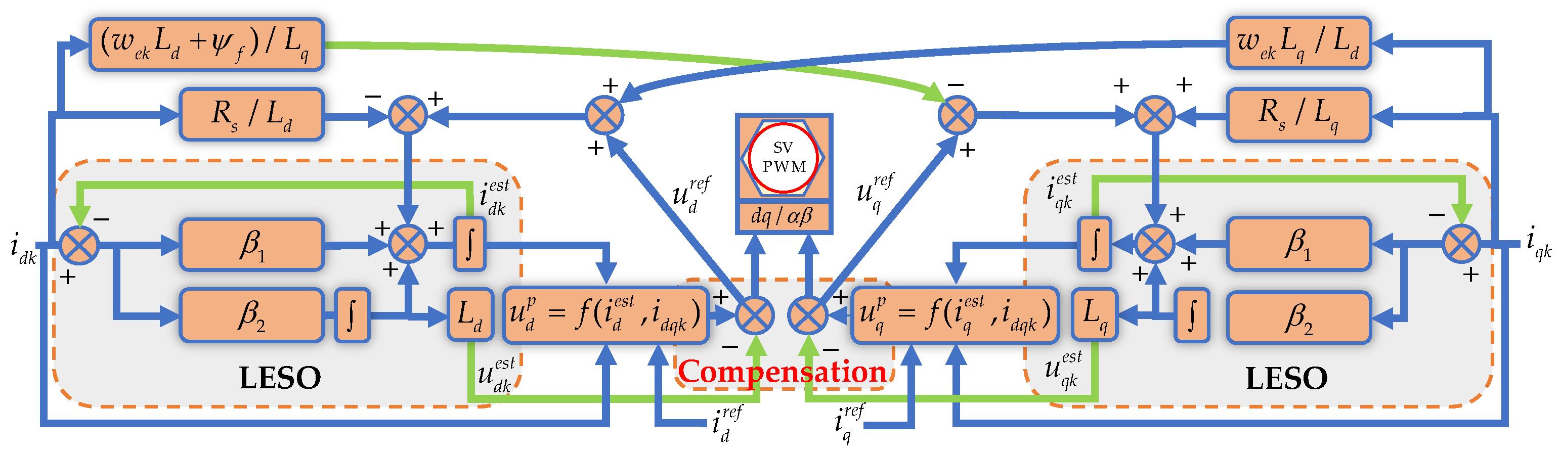
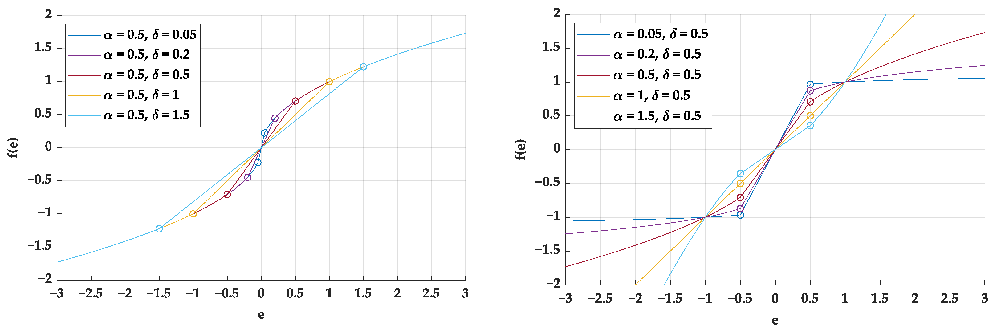
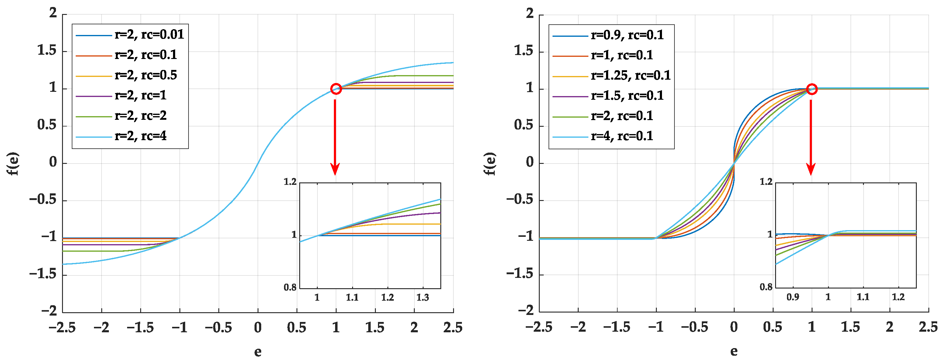
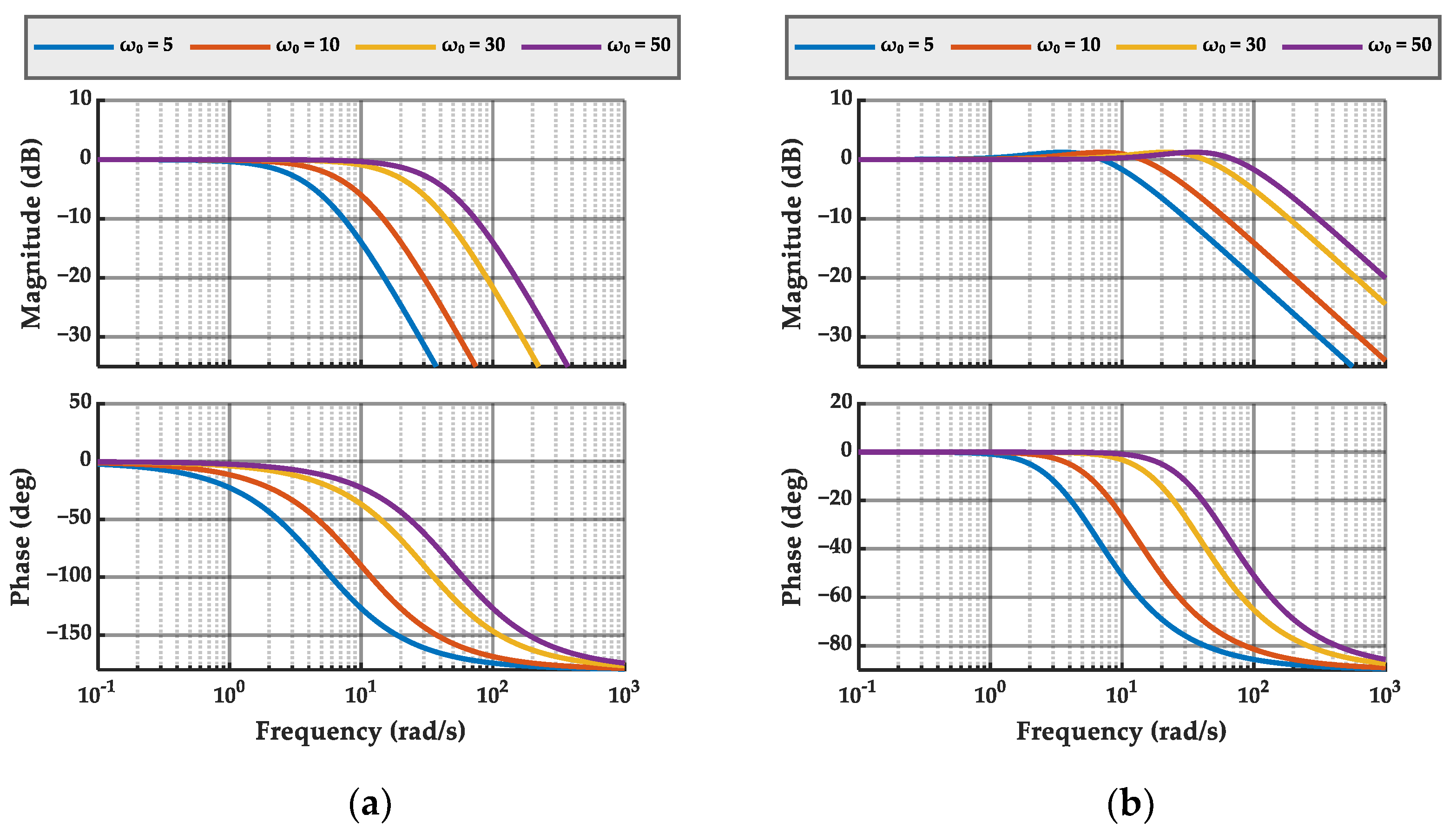
3.3. Proposed NESO Method Analysis

Conventional linear ESOs exhibit limited capability in nonlinear disturbance observation due to their fixed-gain structure, necessitating design improvements. To address this, a nonlinear ESO was introduced, which implements segmented error processing through nonlinear functions. The conventional nonlinear function is defined in Equation (20):
F a l ( e , α , δ ) = e δ 1 α , e δ s i g n ( e ) e α , e > δ
Figure 4 employs the controlled variable method to visualize Fal function profiles under different parameters, with critical data points explicitly annotated at the piecewise function transition regions. By designing the nonlinear factor α < 1, this configuration achieves dynamic gain adjustment characterized by “large-error small-gain, small-error large-gain” behavior.
Figure 4 demonstrates that the conventional Fal function maintains continuity at transition points but lacks differentiability, which may induce system chattering during regulation processes. To address this limitation, a novel Continuously Differentiable Fal (CFal) function is proposed as an enhanced modification:
C F a l ( e ) = y 1 · s i g n ( e ) , i f e 1 y 3 · s i g n ( e ) , i f e x c y 2 · s i g n ( e ) , e l s e a = 2 r 2 1 + 1 2 , b = 2 r 2 1 1 2 θ = arctan ( b a ) Δ x c = r c cos ( π 2 θ ) , Δ y c = r c sin ( π 2 θ ) x c = 1 + Δ x c , y c = 1 Δ y c y 1 = r 2 ( e a s i g n ( e ) ) 2 b y 2 = r c 2 ( e x c s i g n ( e ) ) 2 + y c y 3 = 1 + r c Δ y c
Based on the mathematical expressions of the CFal and Fal functions, the following analytical relationship holds: s i g n [ F a l ( x , α , δ ) ] = s i g n [ C F a l ( x , r ) ] . The Fal function and CFal function exhibit identical convergence directions. When the condition δ α < s i g n ( δ ) ( y 1 ) is satisfied, throughout interval e < 1 , e ˙ = C F a l ( e , r ) demonstrates faster convergence than e ˙ = F a l ( e , α , δ ) at every point. The CFal Function Profile is shown in Figure 5:
The parameter selection is governed by the existence condition of real-number solutions, yielding the following:
2 r 2 1 0 r 2 ( e a s i g n ( e ) ) 2 0 r c 2 ( e x c s i g n ( e ) ) 2 0 r 2 / 2 , r c > 0
Taking the dq-axis current prediction as a case study, the nonlinear function is integrated into the conventional ESO architecture as formulated in Equation (23):
e d = i d ( k ) i d e s t ( k ) , e q = i q ( k ) i q e s t ( k ) i d e s t ( k + 1 ) = i d e s t ( k ) R ^ s L ^ d T s i d ( k ) + ω e ( k ) L ^ q L ^ d T s i q ( k ) + T s L ^ d u d ( k ) + T s β 1 C F al ( r , r c , e d ) + T s L ^ d                                             × u d e s t ( k ) i q e s t ( k + 1 ) = i q e s t ( k ) R ^ s L ^ q T s i q ( k ) ω e ( k ) T s [ L ^ d L ^ q i d ( k ) + ψ ^ f L ^ q ] + T s L ^ q u q ( k ) + T s β 1 C F al ( r , r c , e q ) +                                             × u q e s t ( k ) T s L ^ q

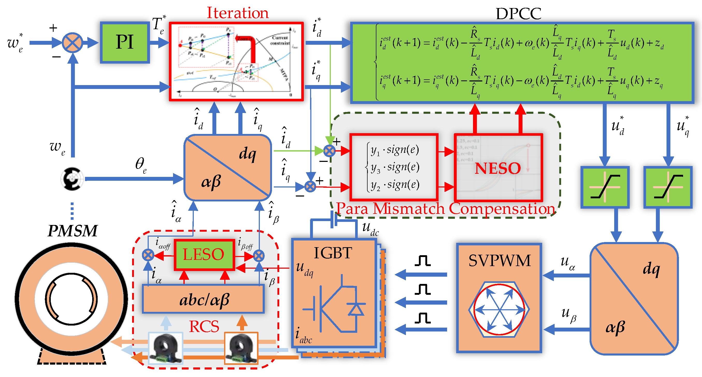
4. MCESO Architecture and Robustness Analysis

The following section will construct a comprehensive evaluation framework that integrates the algorithms from the preceding two sections. The proposed MCESO algorithm samples bias disturbances in the αβ-frame and observes predictive disturbances in the dq-frame, its structure is shown in Figure 6.
Under motor parameter mismatch conditions, all ESO parameters undergo adaptive adjustments. Building on Equation (8), with analogous processing applied to Equation (15), the total disturbance term is formulated as:
d α = Δ R s i α Resistance   error + R s Δ i α + L q d Δ i α d t Sensor   bias + L q d Δ i α d t Inductance   error                                 + [ ( Δ L d Δ L q ) ω e i d + ( L d L q ) ω e Δ i d + Δ ψ f ω e ] sin θ r Flux   and   cross - coupling   disturbance d β = Δ R s i β Resistance   error + R s Δ i β + L q d Δ i β d t Sensor   bias + L q d Δ i β d t Inductance   error                             [ ( Δ L d Δ L q ) ω e i d + ( L d L q ) ω e Δ i d + Δ ψ f ω e ] cos θ r Flux   and   cross - coupling   disturbance
Equation (5) treats the bias error as a low-frequency component and further decomposes the total disturbance into DC and AC components:
d α d c = R s Δ i α , d α a c = d α d α d c d β d c = R s Δ i β , d β a c = d α d β d c
Building upon this analysis, the bandwidth-oriented parameter tuning methodology is implemented as follows:
i ^ α o f f i α o f f = w 0 2 s 2 + 2 w 0 s + w 0 2
The corresponding Bode diagram (Figure 7a) reveals a low-pass filtering relationship between the observed and actual disturbances. Consequently, the front-stage ESO in MCESO requires lower bandwidth to avoid introducing AC errors. The simulation results are shown as follows. Figure 8(a1–a3) display three-phase current waveforms, (a1) startup current, (a2) uncompensated waveform, and (a3) compensated waveform; (b1)–(b2) present α-axis current profiles; while (c) illustrates the observed current bias, with Figure 8, Figure 9, Figure 10 and Figure 11 following analogous definitions.
Based on the ESO architecture, the transfer function between the observed and actual currents is formulated as follows:
G e α = 2 ω 0 s + w 0 2 s 2 + 2 ω 0 s + w 0 2
The corresponding Bode plots in Figure 7b exhibit a minor resonance peak in the magnitude-frequency response alongside phase lag. Subplots (b2) in Figure 8 (bandwidth: 5 rad/s) and Figure 9 (bandwidth: 50 rad/s) demonstrate discernible amplitude and phase deviations between the observed and actual currents. Simulations are conducted at a fundamental current frequency of 125 Hz. The results indicate a robust steady-state error compensation across both bandwidth configurations. Notably, the dynamic response accelerates significantly with increased bandwidth—convergence times approximate 0.5 s at 5 rad/s and 0.15 s at 50 rad/s. However, the fundamental component of the sampling errors in observed values escalates proportionally with bandwidth.
The zoomed view in Figure 9c distinctly reveals a 125 Hz periodic component, consistent with the Inductance Error term in Equation (24). Mechanistically, the residual fundamental component phenomenon originates from the widened passband in high-bandwidth systems, which compromises the effective attenuation of harmonic components beyond the cutoff frequency.
Under motor parameter mismatch conditions, inductance errors deteriorate observation accuracy more severely than other parameter deviations. The disturbances induced by inductance errors are encapsulated in the terms Flux and Cross-coupling Disturbance (FCD) of Equation (24), manifesting as AC disturbances.
In the simulation with a twofold q-axis inductance mismatch, Figure 10 shows the waveforms at a bandwidth of 50 rad/s, and Figure 11 displays those at 10 rad/s. These results demonstrate that as the bandwidth increases, the system stability progressively deteriorates under q-axis inductance mismatch disturbances, ultimately leading to instability. In conclusion, to ensure superior observation performance, the front-stage ESO requires a lower bandwidth to attenuate high-frequency disturbances (term FCD) through filtering.

5. Experimental Results and Discussion

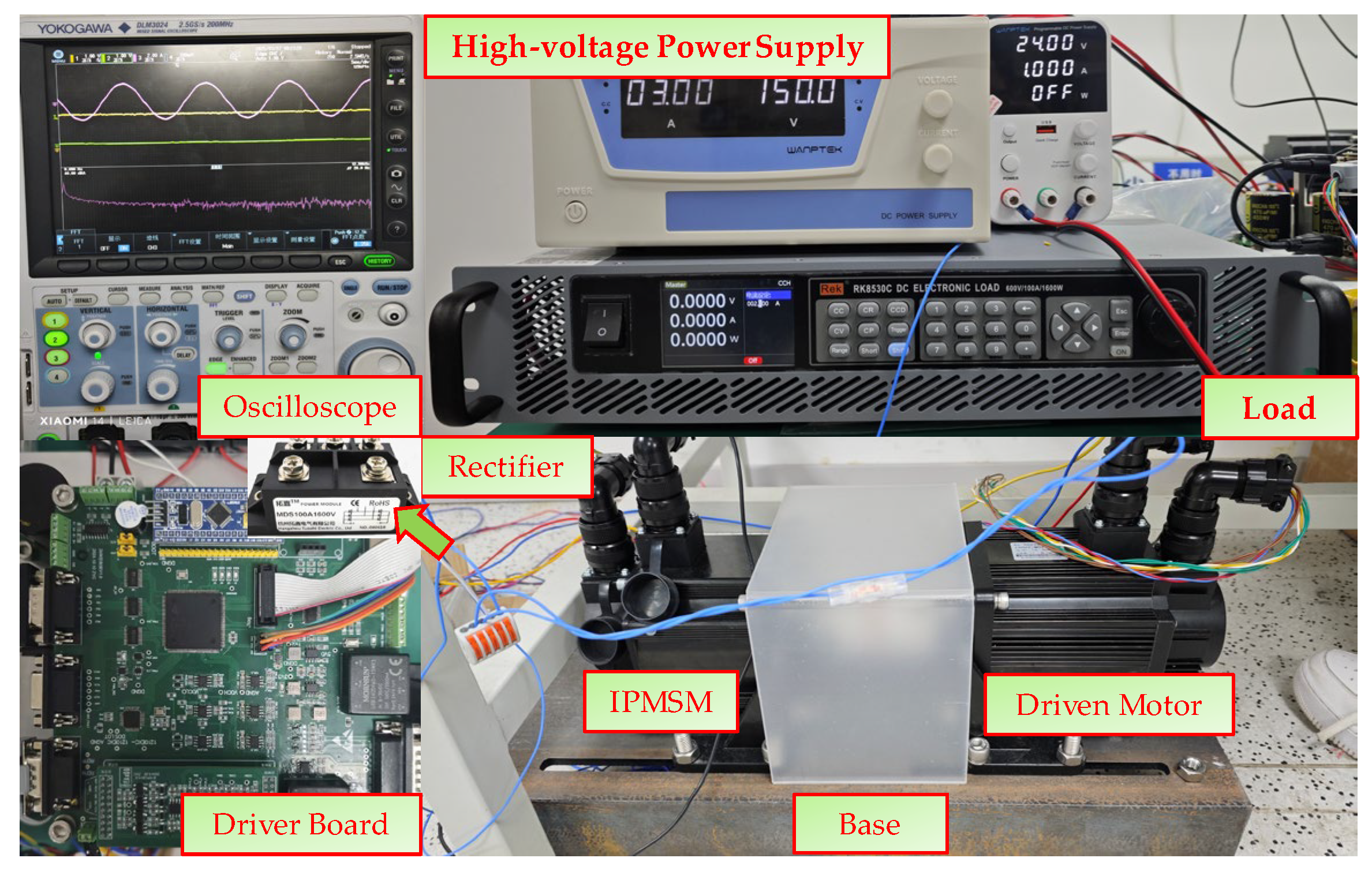
5.1. Introduction to Experimental Equipment

To validate the effectiveness of the proposed high-speed full-operating-range IPMSM control strategy with fast response and enhanced robustness based on MCESO, a series of experimental tests were conducted. The experimental setup, as illustrated in Figure 12, comprises a 500 W interior permanent magnet synchronous motor (IPMSM), a custom-designed motor drive, and ancillary instrumentation, including a power supply and oscilloscope. The proposed control scheme is implemented on a DSP TMS320F28377 controller.
Experimental data were acquired using a Yokogawa DLM3024 oscilloscope, with the IPMSM drive parameters detailed in Table 1. The three-phase inverter prototype incorporates six-pack IGBT modules (FS50W1T7, 1200 V/50 A) with integrated temperature monitoring, operating at 10 kHz switching frequency through DSP-controlled PWM drivers. Motor loading was implemented via a back-to-back motor dynamometer platform, where the generated electrical energy from the slave motor is fed into an electronic load through a diode-based passive rectifier. It is explicitly stated that all subsequent references to current loading in this paper pertain to the current values applied by the electronic load.

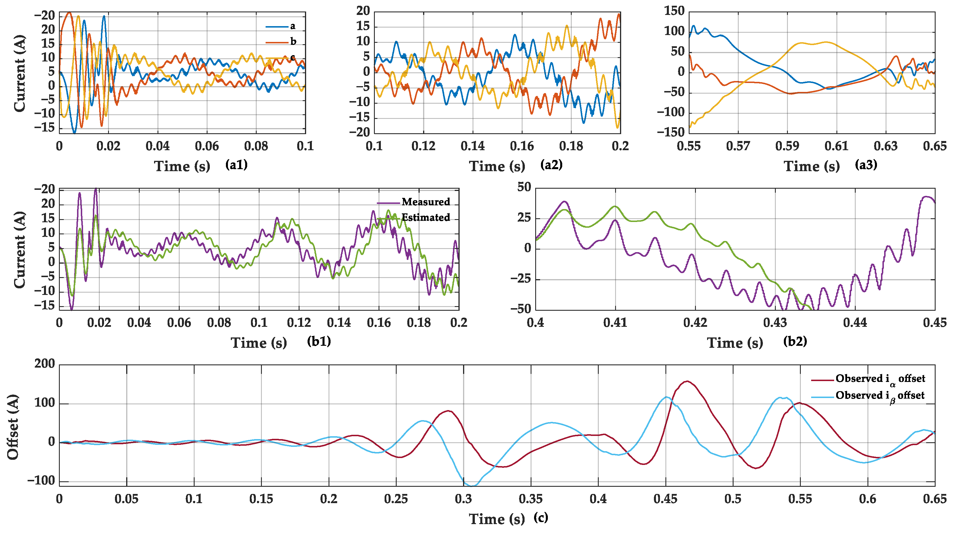
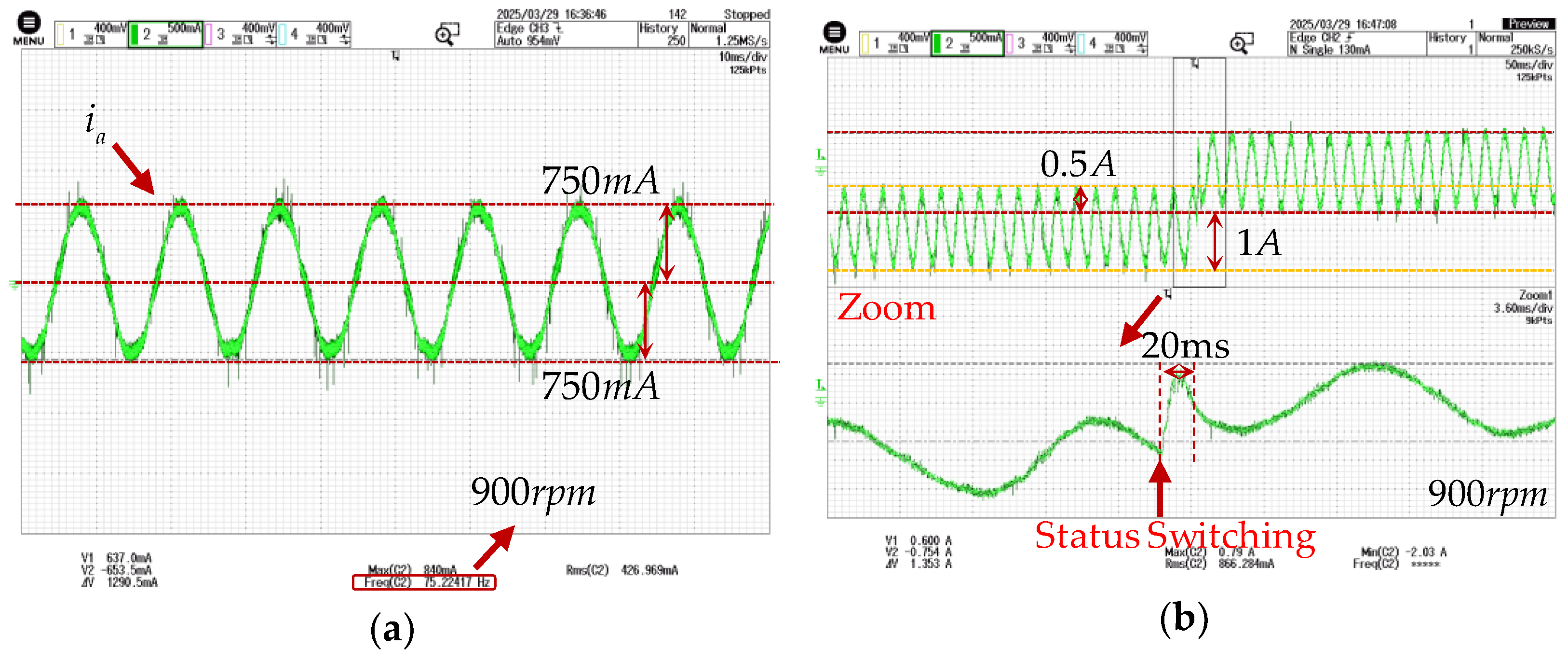
5.2. Experimental Results of Front-Stage MCESO

The DC bus voltage is set to 150 V and the motor achieves a rotational speed of 900 rpm under the proposed algorithm. In accordance with the prior analysis, the observer bandwidth is configured at 10 Hz.
Figure 13 demonstrates the algorithm’s performance under no-load conditions. Figure 13a displays the steady-state Phase A current waveform after algorithm activation, showing no significant offset with a peak value of 750 mA. Measurements were acquired with the oscilloscope in full bandwidth mode, confirming the algorithm introduces no additional current harmonics. Figure 13b compares the dynamic Phase A current waveforms before and after algorithm activation. The experimental results indicate a −1 A bias in the phase current. The peak current reaching approximately 1.3 A exacerbates motor heating and reduces operational efficiency. Following algorithm activation, the sampling error is fully compensated within 20 ms.
Figure 14 demonstrates the algorithm performance under loaded operating conditions. The electronic load applies a 2 A current with a peak-to-peak value of approximately 7 A under identical waveform definitions. Following algorithm activation, the sampling error is fully compensated within 10 ms, demonstrating that current loading facilitates observer-based error compensation.

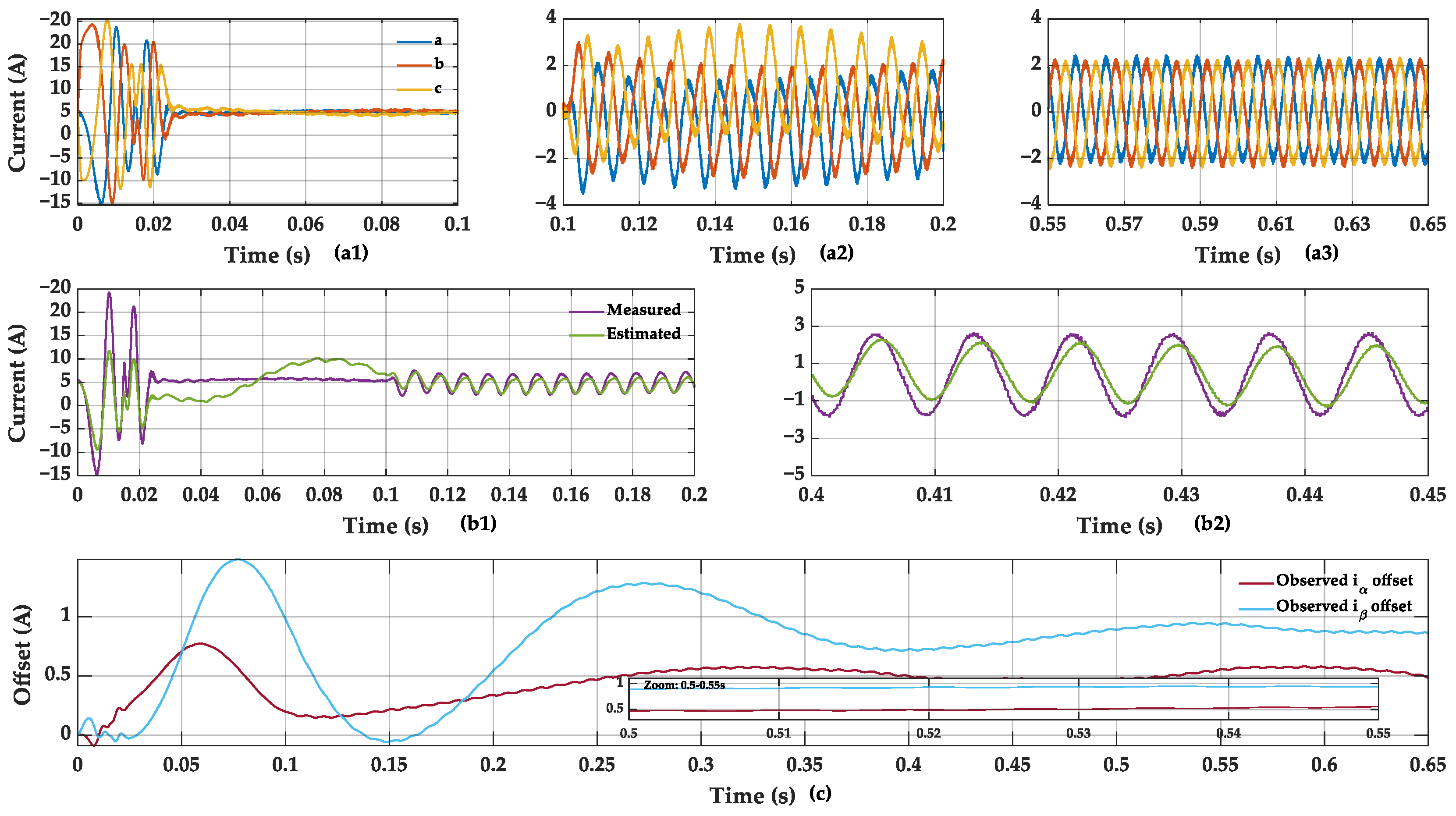
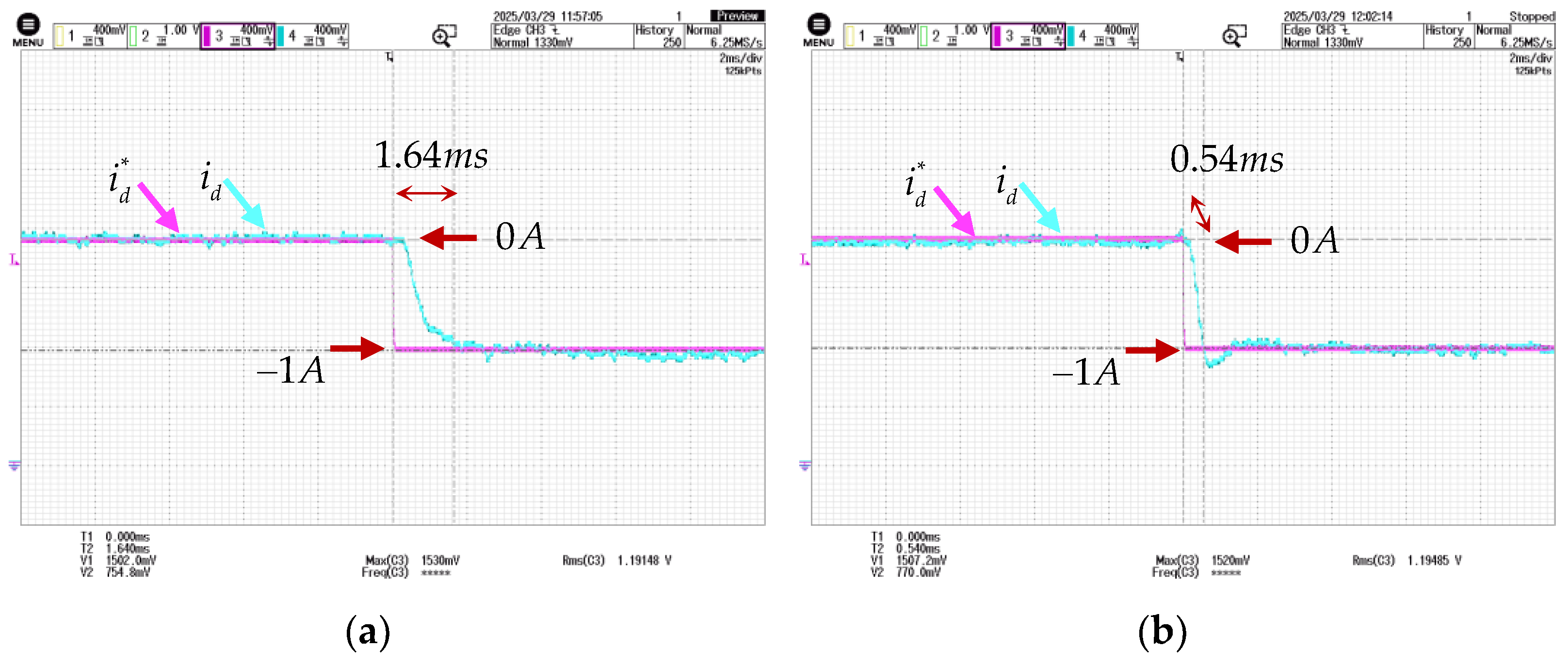
5.3. Experimental Results of Post-Stage MCESO

The post-stage MCESO primarily achieves rapid current tracking. Figure 15 compares the current dynamic response waveforms between PI and MCESO under motor operation at 900 rpm. To isolate variables for analysis, a step change of −1 A was applied to the d-axis current reference, as the q-axis current steps induce torque variations. Figure 15a shows the response waveform under conventional PI control with a settling time of 1.64 ms, while Figure 15b demonstrates the MCESO algorithm reducing the dynamic response time to 0.54 ms, thereby validating its efficacy in enhancing the dynamic response speed.
The conventional deadbeat predictive current control (DPCC) algorithm demonstrates significant parameter sensitivity. Figure 16a presents waveforms under nominal parameter conditions, while Figure 16b shows waveforms under parameter mismatch (twofold inductance deviation). The experimental results reveal that with inductance mismatch, the conventional DPCC exhibits deteriorated current THD (Total Harmonic Distortion), introduces DC offsets and superimposed oscillatory components in dq-axis currents, and induces speed instability. Furthermore, torque ripple intensification is observed under mismatched conditions.
For comparative validation of the MCESO algorithm, experimental waveforms are presented in Figure 17. The test conditions include variable-speed light-load operation at 0.5 A with a DC bus voltage of 150 V. The green trace represents Phase A current. In Figure 17a, the pink trace denotes the q-axis current reference while blue indicates the actual q-axis current. Figure 17b shows the speed reference (pink) versus the actual speed (blue). The experimental results demonstrate that MCESO achieves precise tracking of both current and speed references despite parameter mismatch and sampling bias errors, with a notably rapid dynamic response.

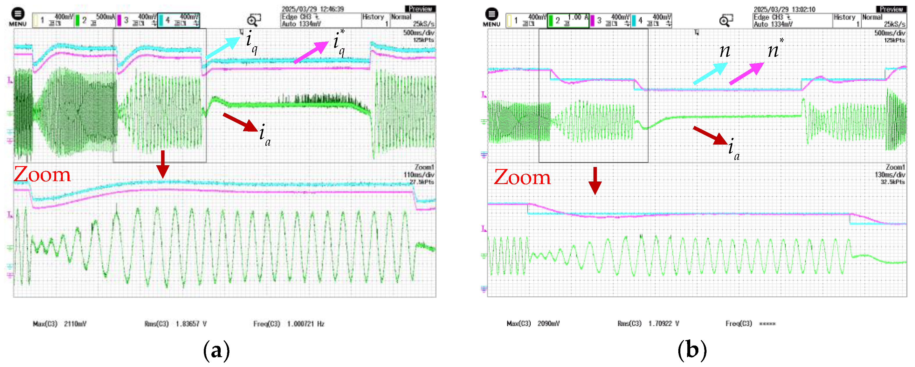
5.4. Experimental Results of MCESO Under Full-Speed-Range Operation

5.4.1. Operation Below Base Speed

IPMSM typically employs MTPA control below base speed. The id = 0 strategy was first applied to verify the q-axis current correspondence with the fundamental current amplitude. Algorithm validation at 150 r/min (12.5 Hz) with a 3 A load confirmed low-speed performance. Both phase currents and dq-axis current waveforms are presented in Figure 18, where the dq-axis currents demonstrate accurate tracking performance of their references while the phase currents maintain undistorted sinusoidal waveforms.
After that, the MTPA operating point reference was generated using the fast projection iteration method from Reference [8], with a DC bus voltage of 150 V and motor speed of 900 rpm under loaded conditions.
Figure 19 illustrates experimental waveforms of conventional PI control under current bias error, revealing a phase current THD of 8.70% and significant dq-axis current pulsations. Figure 20 demonstrates the MCESO-based waveforms, showing bias error compensation and reduced current harmonics to 5.36% THD.

5.4.2. Operation Above Base Speed

Above base speed, the IPMSM employs field-weakening control through d-axis current regulation to mitigate voltage saturation effects, thereby achieving extended speed operation. The field-weakening operating points are determined using the methodology from Reference [8], with experiments conducted under varying DC bus voltages. Test conditions included a DC bus voltage of 150 V and a field-weakening speed of 1350 rpm. Figure 21 shows the conventional PI control waveforms, where significant fluctuations in dq-axis currents are observed, accompanied by a phase current THD of 7.52%.
Furthermore, traditional PI parameter tuning must dynamically account for bandwidth effects, as the electrical frequency corresponding to the given speed in this experiment is 150 Hz. Figure 22 presents current waveforms under different bandwidth configurations. Figure 22a at 100 Hz bandwidth exhibits clear current instability, while Figure 22b at 200 Hz bandwidth demonstrates marginally stabilized operation. These results validate the extreme sensitivity of conventional PI current loop bandwidth configurations in field-weakening scenarios.
Figure 23 demonstrates the performance of MCESO under field-weakening conditions. The experimental setup matches that of Figure 21, with both disturbances (parameter mismatch and sampling bias) present. The results show that under field-weakening operation, the current harmonics are reduced from 7.52% to 4.62% THD, dq-axis current pulsations are minimized, and motor efficiency is improved.
The DC bus voltage is elevated to 200 V for multi-operating condition algorithm validation. Figure 24 displays experimental waveforms of the conventional Linear Extended State Observer (LESO), where the green trace represents Phase A current, blue denotes the actual d-axis current, and purple indicates the field-weakening d-axis reference current. Under this configuration, the d-axis current reaches −2.2 A, reflecting a deepened field-weakening level, with a phase current peak-to-peak value of 6 A. The right subfigure presents FFT analysis of the phase current, revealing a THD of 3.37%.
Figure 25 presents the field-weakening MCESO waveforms under identical definitions as described above; the THD is 3.31%. Notably, both methodologies were experimentally validated under concurrent conditions of current sampling bias errors and predictive control parameter mismatch. Compared to LESO, MCESO achieves significant harmonic suppression in the DC component but exhibits a slight increase in high-frequency band components. This phenomenon arises because the nonlinear function enhances error regulation through variable gain for large/small errors and improves nonlinear disturbance observation capability, yet the switching points of the nonlinear function may introduce additional noise components. In summary, MCESO achieves a 0.06% reduction in the current THD (3.37% minus 3.31%), demonstrating that the proposed algorithm maintains stable operation even under high-speed motor operation and harsh operating conditions.
Last but not least, dynamic performance tests across the full speed range facilitate the validation of overall system reliability. Transient response experiments were carried out under 1 A loading, spanning five speed stages from low to high velocity. Speed transitions were sequentially implemented at 2 s intervals (150, 750, 1350, 1850, 2100, and 1500 r/min). Figure 26 illustrates the corresponding rotational speed and current profiles, where flux-weakening mode activation is observed at 1850 and 2100 r/min. The experimental validation confirms the algorithm’s capability to maintain stable and robust control performance during abrupt load transients.

6. Conclusions

This paper proposes a Multi-axis Collaborative Extended State Observer (MCESO) control strategy to achieve fast-response and high-robustness operation of IPMSMs across wide speed ranges. By analyzing the predictive model and introducing augmented state variables into the state equations, the strategy observes system states and applies closed-loop compensation to address total disturbances under parameter mismatch and current sampling errors. Through Bode diagram analysis of disturbance signals and parameter mismatch, the frequency-dependent relationship between MCESO and disturbances was rigorously investigated, validating the dual advantages of high robustness and rapid dynamic responses. The experimental results demonstrated the algorithm’s effectiveness in both MTPA and flux-weakening regions, enabling reliable operation in harsh conditions while enhancing system performance. Regarding current harmonic suppression performance, the THD in the MTPA region was reduced from 8.70% (conventional methods) to 5.36%, while in the flux-weakening region, the THD achieved a reduction of 2.9 percentage points, optimized to 4.62%.

Author Contributions

Formal analysis, W.Z.; Investigation, Y.Z. and Y.L.; Methodology, W.Z.; Resources, P.Z.; Software, P.Z.; Supervision, P.Z. and Y.L.; Validation, Y.Z.; Writing—original draft, Y.Z.; Writing—review and editing, W.Z. All authors have read and agreed to the published version of the manuscript.

Funding

This work is sponsored by the National Natural Science Foundation of China (No. 52207043).

Data Availability Statement

All original contributions are detailed in this article. Inquiries may be directed to the corresponding author.

Conflicts of Interest

The authors declare no conflicts of interest.

Nomenclature

u 3 s , i 3 s , e 3 s Three-phase voltage, current, back EMF.
u α , u β , i α , i β Alpha-beta axis voltage and current.
u d , u q , i d , i q Dq axis voltage and current.
p Differential operator.
R s , L s Phase resistance and inductance.
L α , L α β , L β Alpha-beta axis inductance.
L d , L q , ψ f Dq axis inductance and permanent magnet flux linkage.
ω e , θ e ( θ r ) Point angular velocity and electrical angle.
i a b c m , i α β m , i d q m Measured current in different coordinate systems.
i a b c a c t , i α β a c t , i d q a c t The actual current in different coordinate systems.
i a b c o f f , i α β o f f , i d q o f f Current bias in different coordinate systems.
T e , T e m , T e o f f Electromagnetic torque, measuring torque, torque bias.
i ^ α m , i ^ α o f f , i ^ β m , i ^ β o f f Alpha-beta axis current and bias estimation.
e α , e β , e d , e q The real value minus the observed value.
K p , K i Pi parameters.
δ R s , δ L s Resistance and inductance mismatch variation.
z α β d q Extended state variables—actual.
z ^ α β d q Extended state variables—estimates.
β 1 , β 2 , ω c ESO coefficient.
T s Interrupt cycle.
i d r e f , i q r e f Dq axis current reference given value.
Δ R s , Δ L d q Resistance-inductance mismatch value under dq axis.
u n o i s e Equivalent value of nonlinear voltage disturbance.
u d e s t , u q e s t , i d e s t , i q e s t Estimate dq axis voltage and current.
e , α , δ , y 123 , a , b , x c , y c non-linear function parameter.
d α , d β Alpha-beta axis lumped disturbance.
d d c , d a c DC disturbance and AC disturbance.
Δ i α , Δ i β Alpha-beta axis current error.

Appendix A

Section I: The state Equation (11) has been restructured as Equation (A1):
d i α m d t d i ^ α m d t = R s L q ( i α m i ^ α m ) β 1 ( i α m i ^ α m ) + ( z α z ^ α ) d z α d t d z ^ α d t = β 2 ( i α m i ^ α m ) + d z α d t
It is noteworthy that Equation (11) above represents the error equation, where the first expression is derived by subtracting the observation equation from the original model’s state equation. Taking the alpha-axis as an example, the original model’s state equation is formulated as follows:
d i α m d t = R s L q i α m + 1 L q u α 1 L q e α + z α
The observation equation is given by the following:
d i ^ α m d t = R s L q i ^ α m + 1 L q u α 1 L q e α + β 1 ( i α m i ^ α m ) + z ^ α
The second expression in Equation (11) is derived through a straightforward algebraic transformation of the following equation:
d z ^ α d t = β 2 ( i α m i ^ α m )
Define the current estimation error and disturbance estimation error as the following:
ε 1 = i α m i ^ α m ε 2 = z α z ^ α
By neglecting the stator resistance, the error state equation (where A is the system matrix) can be expressed as the following:
ε ˙ 1 ε ˙ 2 = β 1 1 β 2 0 A ε 1 ε 2 + 0 1 z ˙ α
The characteristic equation is as follows:
det ( s I A ) = s 2 + β 1 s + β 2
So, if the poles are located in the left half-plane, it can lead to ε 1 , ε 2 tending to 0. This demonstrates that the observed variables can achieve finite time convergence to their true values. Furthermore, configure β1 = 2ωₑ, β2 = ωₑ2. This configuration allows the disturbance observer to function as a second-order low-pass filter, from which the transfer function can be derived as follows.
Section II: By taking the second derivative of Equation (A4), we obtain the following:
1 β 2 z ^ ¨ α = β 2 ( i ˙ α m i ^ ˙ α m )
By combining Equations (A1) and (A8), we derive the following expression:
1 β 2 z ^ ¨ α = β 1 1 β 2 z ^ ˙ α + ( z α z ^ α )
Based on the relationship between the extended state and current sampling bias, we obtain the following:
z ^ α = R s L q i ^ α o f f , z α = R s L q i α o f f
Consequently, the transfer function corresponding to Equation (11) can be derived as follows:
1 β 2 i ^ ¨ α o f f = β 1 1 β 2 i ^ ˙ α o f f + ( i α o f f i ^ α o f f ) i ^ α o f f i α o f f = β 2 s 2 + β 1 s + β 2 = ω e 2 s 2 + 2 ω e s + ω e 2
Configuring the observer bandwidth as β1 = 2ωₑ, β2 = ωₑ2. This configuration ensures that the relationship between the observed disturbance and the actual disturbance is governed by a second-order low-pass filter.

References

  1. Zhou, M.; Fei, X.; Xu, W.; Cai, W.; Xie, Y.; Qiu, Z. Adaptive Gain-Based Double-Loop Full-Order Terminal Sliding Mode Control of a Surface-Mounted PMSM System. Energies 2025, 18, 2112. [Google Scholar] [CrossRef]
  2. Zhu, B.; Zhu, D.; Tao, T. Model-Free Adaptive Fuzzy Sliding-Mode Observer Control for PMSM. Energies 2025, 18, 1877. [Google Scholar] [CrossRef]
  3. Zou, J.; Zhu, P.; Zhang, W.; Xu, Y.; Zou, J. Software-Based Resolver-to-Digital Converter Using an αβγ Filter. IEEE Trans. Instrum. Meas. 2024, 73, 7502211. [Google Scholar] [CrossRef]
  4. Zhai, Y.; Zhang, W.; Xu, Y.; Zou, J. Parameter Identification of Permanent Magnet Synchronous Motor Based on Long Short Term Memory Neural Network. In Proceedings of the 2024 IEEE 10th International Power Electronics and Motion Control Conference (IPEMC2024-ECCE Asia), Chengdu, China, 17 May 2024; IEEE: Piscataway, NJ, USA, 2024; pp. 3873–3878. [Google Scholar]
  5. Cheng, S.; Zhang, W.; Wang, J.; Ji, Q. Research on a Sensorless Control System for Dual-Branch Permanent Magnet Synchronous Motor with a Nonlinear Observer Based on Parameter Identification. In Proceedings of the 2024 7th International Conference on Power and Energy Applications (ICPEA), Taiyuan, China, 18 October 2024; IEEE: Piscataway, NJ, USA, 2024; pp. 240–245. [Google Scholar]
  6. Cao, M.; Egashira, J.; Kaneko, K. High Efficiency Control of IPMSM for Electric Motorcycles. In Proceedings of the 2009 IEEE 6th International Power Electronics and Motion Control Conference, Wuhan, China, 17–20 May 2009; IEEE: Piscataway, NJ, USA, 2009; pp. 1893–1897. [Google Scholar]
  7. Sun, T.; Wang, J. Extension of Virtual-Signal-Injection-Based MTPA Control for Interior Permanent-Magnet Synchronous Machine Drives Into the Field-Weakening Region. IEEE Trans. Ind. Electron. 2015, 62, 6809–6817. [Google Scholar] [CrossRef]
  8. Xia, Z.; Filho, S.R.; Xiao, D.; Fang, G.; Sun, Y.; Wiseman, J.; Emadi, A. Computation-Efficient Online Optimal Tracking Method for Permanent Magnet Synchronous Machine Drives for MTPA and Flux-Weakening Operations. IEEE J. Emerg. Sel. Top. Power Electron. 2021, 9, 5341–5353. [Google Scholar] [CrossRef]
  9. Xu, Q.; Cai, L. Developing an Approach in Calculating Reference Currents for Field-Weakening Control. IEEE Trans. Transp. Electrif. 2023, 9, 60–74. [Google Scholar] [CrossRef]
  10. Zhang, X.; Fang, S.; Zhang, H. Predictive Current Error Compensation Based Strong Robust Model Predictive Control for PMSM Drive Systems. IEEE Trans. Ind. Electron. 2024, 71, 15280–15289. [Google Scholar] [CrossRef]
  11. Fan, Y.; Chen, J.; Zhang, Q.; Cheng, M. An Improved Inertia Disturbance Suppression Method for PMSM Based on Disturbance Observer and Two-Degree-of-Freedom PI Controller. IEEE Trans. Power Electron. 2023, 38, 3590–3599. [Google Scholar] [CrossRef]
  12. Xue, W.; Madonski, R.; Lakomy, K.; Gao, Z.; Huang, Y. Add-On Module of Active Disturbance Rejection for Set-Point Tracking of Motion Control Systems. IEEE Trans. Ind. Appl. 2017, 53, 4028–4040. [Google Scholar] [CrossRef]
  13. Yan, Z.; Deng, S.; Yang, Z.; Zhao, X.; Yang, N.; Lu, Y. Improved Nonlinear Active Disturbance Rejection Control for a Continuous-Wave Pulse Generator with Cascaded Extended State Observer. Control Eng. Pract. 2024, 146, 105897. [Google Scholar] [CrossRef]
  14. Zhang, Y.; Yin, Z.; Bai, C.; Wang, G.; Liu, J. A Rotor Position and Speed Estimation Method Using an Improved Linear Extended State Observer for IPMSM Sensorless Drives. IEEE Trans. Power Electron. 2021, 36, 14062–14073. [Google Scholar] [CrossRef]
  15. Zeng, X.; Wang, W.; Wang, H. Adaptive PI and RBFNN PID Current Decoupling Controller for Permanent Magnet Synchronous Motor Drives: Hardware-Validated Results. Energies 2022, 15, 6353. [Google Scholar] [CrossRef]
  16. Yu, K.; Wang, Z.; Hua, W.; Cheng, M. Robust Cascaded Deadbeat Predictive Control for Dual Three-Phase Variable-Flux PMSM Considering Intrinsic Delay in Speed Loop. IEEE Trans. Ind. Electron. 2022, 69, 12107–12118. [Google Scholar] [CrossRef]
  17. Zhong, L.; Rahman, M.F.; Hu, W.Y.; Lim, K.W. Analysis of Direct Torque Control in Permanent Magnet Synchronous Motor Drives. IEEE Trans. Power Electron. 1997, 12, 528–536. [Google Scholar] [CrossRef]
  18. Casadei, D.; Profumo, F.; Serra, G.; Tani, A. FOC and DTC: Two Viable Schemes for Induction Motors Torque Control. IEEE Trans. Power Electron. 2002, 17, 779–787. [Google Scholar] [CrossRef]
  19. Sheikh, I.; Krishna, M.S.R.; Seshadrinath, J. Performance Comparison of FOC and DTC Techniques for SynRM in EV Applications. In Proceedings of the 2024 IEEE International Conference on Power Electronics, Drives and Energy Systems (PEDES), Mangalore, India, 18 December 2024; IEEE: Piscataway, NJ, USA, 2024; pp. 1–6. [Google Scholar]
  20. Cortes, P.; Kazmierkowski, M.P.; Kennel, R.M.; Quevedo, D.E.; Rodriguez, J. Predictive Control in Power Electronics and Drives. IEEE Trans. Ind. Electron. 2008, 55, 4312–4324. [Google Scholar] [CrossRef]
  21. Morel, F.; Lin-Shi, X.; Retif, J.-M.; Allard, B.; Buttay, C. A Comparative Study of Predictive Current Control Schemes for a Permanent-Magnet Synchronous Machine Drive. IEEE Trans. Ind. Electron. 2009, 56, 2715–2728. [Google Scholar] [CrossRef]
  22. Moon, H.T.; Kim, H.S.; Youn, M.J. A Discrete-Time Predictive Current Control for PMSM. IEEE Trans. Power Electron. 2003, 18, 464–472. [Google Scholar] [CrossRef]
  23. Zhang, Y.; Xu, D.; Liu, J.; Gao, S.; Xu, W. Performance Improvement of Model-Predictive Current Control of Permanent Magnet Synchronous Motor Drives. IEEE Trans. Ind. Appl. 2017, 53, 3683–3695. [Google Scholar] [CrossRef]
  24. Zhang, Y.; Xu, D.; Huang, L. Generalized Multiple-Vector-Based Model Predictive Control for PMSM Drives. IEEE Trans. Ind. Electron. 2018, 65, 9356–9366. [Google Scholar] [CrossRef]
  25. Wei, Y.; Young, H.; Ke, D.; Wang, F.; Qi, H.; Rodríguez, J. Model-Free Predictive Control Using Sinusoidal Generalized Universal Model for PMSM Drives. IEEE Trans. Ind. Electron. 2024, 71, 13720–13731. [Google Scholar] [CrossRef]
  26. Zhang, X.; Zhang, L.; Zhang, Y. Model Predictive Current Control for PMSM Drives With Parameter Robustness Improvement. IEEE Trans. Power Electron. 2019, 34, 1645–1657. [Google Scholar] [CrossRef]
  27. Moreno, J.C.; Espi Huerta, J.M.; Gil, R.G.; Gonzalez, S.A. A Robust Predictive Current Control for Three-Phase Grid-Connected Inverters. IEEE Trans. Ind. Electron. 2009, 56, 1993–2004. [Google Scholar] [CrossRef]
  28. Young, H.A.; Perez, M.A.; Rodriguez, J. Analysis of Finite-Control-Set Model Predictive Current Control With Model Parameter Mismatch in a Three-Phase Inverter. IEEE Trans. Ind. Electron. 2016, 63, 3100–3107. [Google Scholar] [CrossRef]
  29. Attaianese, C.; D’Arpino, M.; Monaco, M.D.; Noia, L.P.D. Model-Based Detection and Estimation of DC Offset of Phase Current Sensors for Field Oriented PMSM Drives. IEEE Trans. Ind. Electron. 2023, 70, 6316–6325. [Google Scholar] [CrossRef]
  30. Kang, Y.G.; Reigosa, D.D. Dq-Transformed Error and Current Sensing Error Effects on Self-Sensing Control. IEEE J. Emerg. Sel. Top. Power Electron. 2022, 10, 1935–1945. [Google Scholar] [CrossRef]
  31. Zhang, Q.; Guo, H.; Liu, Y.; Guo, C.; Zhang, F.; Zhang, Z.; Li, G. A Novel Error-Injected Solution for Compensation of Current Measurement Errors in PMSM Drive. IEEE Trans. Ind. Electron. 2023, 70, 4608–4619. [Google Scholar] [CrossRef]
  32. Zuo, Y.; Wang, H.; Ge, X.; Zuo, Y.; Woldegiorgis, A.T.; Feng, X.; Lee, C.H.T. A Novel Current Measurement Offset Error Compensation Method Based on the Adaptive Extended State Observer for IPMSM Drives. IEEE Trans. Ind. Electron. 2024, 71, 3371–3382. [Google Scholar] [CrossRef]
  33. Lee, S.; Kim, H.; Lee, K. Current Measurement Offset Error Compensation in Vector-Controlled SPMSM Drive Systems. IEEE J. Emerg. Sel. Top. Power Electron. 2022, 10, 2619–2628. [Google Scholar] [CrossRef]
Figure 1. Single-Factor Current Bias Error Compensation Architecture. (a) Traditional PI structure; (b) Linear extended state observer structure.
Energies 18 02938 g001
Figure 2. Block Diagram of DPCC vs. PI Current Loop Architecture.
Energies 18 02938 g002
Figure 3. Block Diagram of ESO-Based DPCC Algorithm.
Energies 18 02938 g003
Figure 4. Conventional Fal Function Picture.
Energies 18 02938 g004
Figure 5. CFal Function Picture.
Energies 18 02938 g005
Figure 6. Block Diagram of MCESO Architecture.
Energies 18 02938 g006
Figure 7. Bode Diagram Analysis of Observed Current and Disturbance. (a) Observation disturbance transfer function. (b) Observing the actual current transfer function.
Energies 18 02938 g007
Figure 8. Simulated Waveforms at 5 rad/s Bandwidth Under Parameter-Mismatch-Free Conditions. (a1) 0 to 0.1 s three-phase current. (a2) 0.1 to 0.2 s three-phase current. (a3) 0.55 to 0.65 s three-phase current. (b1) 0 to 0.2 s actual and observed alpha axis current. (b2) 0.4 to 0.45 s actual and observed alpha axis current. (c) Actual and observed alpha axis perturbations.
Energies 18 02938 g008
Figure 9. Simulated Waveforms at 50 rad/s Bandwidth Under Parameter-Mismatch-Free Conditions. (a1) 0 to 0.1 s three-phase current. (a2) 0.1 to 0.2 s three-phase current. (a3) 0.55 to 0.65 s three-phase current. (b1) 0 to 0.2 s actual and observed alpha axis current. (b2) 0.4 to 0.45 s actual and observed alpha axis current. (c) Actual and observed alpha axis perturbations.
Energies 18 02938 g009
Figure 10. Simulation Waveforms with Inductance Mismatch Under Doubled Bandwidth (50 rad/s). (a1) 0 to 0.1 s three-phase current. (a2) 0.1 to 0.2 s three-phase current. (a3) 0.55 to 0.65 s three-phase current. (b1) 0 to 0.2 s actual and observed alpha axis current. (b2) 0.4 to 0.45 s actual and observed alpha axis current. (c) Actual and observed alpha axis perturbations.
Energies 18 02938 g010
Figure 11. Simulation Waveforms with Inductance Mismatch Under Doubled Bandwidth (10 rad/s). (a1) 0 to 0.1 s three-phase current. (a2) 0.1 to 0.2 s three-phase current. (a3) 0.55 to 0.65 s three-phase current. (b1) 0 to 0.2 s actual and observed alpha axis current. (b2) 0.4 to 0.45 s actual and observed alpha axis current. (c) Actual and observed alpha axis perturbations.
Energies 18 02938 g011
Figure 12. Experimental Platform of the IPMSM Drive System.
Energies 18 02938 g012
Figure 13. The Test Results of the Motor Under No-Load Condition. (a) Compensate steady-state results. (b) Dynamic compensation results.
Energies 18 02938 g013
Figure 14. The Test Results of the Motor Under Loading Condition. (a) Compensate steady-state results. (b) Dynamic compensation results.
Energies 18 02938 g014
Figure 15. Current Dynamic Response: PI vs. MCESO Waveforms. (a) Traditional PI. (b) Model predictive control.
Energies 18 02938 g015
Figure 16. Conventional DPCC: Waveforms under Nominal vs. Mismatched Conditions. (a) No mismatch. (b) Parameter mismatch.
Energies 18 02938 g016
Figure 17. Predictive Current Waveforms with MCESO under Parameter Mismatch. (a) Current waveform. (b) Speed waveform.
Energies 18 02938 g017
Figure 18. id = 0 Control with Conventional MCESO Under Sampling Collective Disturbance.
Energies 18 02938 g018
Figure 19. MTPA Control with Conventional PI Under Sampling Bias Error.
Energies 18 02938 g019
Figure 20. MTPA Control with MCESO Under Sampling Collective Disturbance.
Energies 18 02938 g020
Figure 21. Flux Weakening Control with Conventional PI.
Energies 18 02938 g021
Figure 22. Different bandwidth results under traditional PI weak magnetic field. (a) bandwidth deficiency. (b) Sufficient bandwidth.
Energies 18 02938 g022
Figure 23. Flux Weakening Control with MCESO (150 V).
Energies 18 02938 g023
Figure 24. Flux Weakening Control with LESO.
Energies 18 02938 g024
Figure 25. Flux Weakening Control with MCESO (200 V).
Energies 18 02938 g025
Figure 26. Full-Speed-Range Dynamic Test with MCESO.
Energies 18 02938 g026
Table 1. Parameters of the IPMSM.
Motor SpecificationValueMotor SpecificationValue
Motor Type IPMSMStator Resistance 0.425 Ω
Rated Power 500 WD-axis Inductance7.8 mH
Rated Current4 AQ-axis Inductance10.5 mH
Rated Speed2000 rpmFlux Linkage0.12475 Wb
Rated Voltage200 VSwitching Frequency10 kHz
Pairs of Poles5Rotational Inertia0.9 × 10−3 Kg·m2
Disclaimer/Publisher’s Note: The statements, opinions and data contained in all publications are solely those of the individual author(s) and contributor(s) and not of MDPI and/or the editor(s). MDPI and/or the editor(s) disclaim responsibility for any injury to people or property resulting from any ideas, methods, instructions or products referred to in the content.

