Empirical Motion Compensation for Turbulence Intensity Measurement by Floating LiDARs

Abstract

We propose an empirical motion compensation algorithm for a better turbulence intensity (TI) measurement by Floating LiDAR systems (FLSs) with a newly introduced motion parameter, the significant tilt angle ${\theta }_{\alpha ,1/3}$, using four datasets from three different FLSs in Japan. The parameter was compared to other environmental parameters; it was confirmed to well represent various types of buoy motion. A sensitivity assessment was conducted for the error of the FLS’s standard deviation of wind speed to the buoy motion. The strong correlation obtained by the assessment suggests that the error of the FLS TI is dominated by the motion and that it is possible to offset the error by applying the relationship back to the measurement. The corrected TI shows good agreement with that of a reference fixed vertical LiDAR (VL). Moreover, the similarity of the relationships for the same type of VL mounted on different buoys implies that the correction may be VL-specific rather than FLS-specific, and, therefore, universal regardless of the FLS type. The successful validation suggests that the correction based on ${\theta }_{\alpha ,1/3}$ can be applied not only to the future campaign but also to those performed in the past to revitalize numerous existing FLS datasets.

1. Introduction

Floating LiDAR (light detection and ranging) systems (hereinafter referred to as FLSs) have been developed over the past decades and can nowadays replace a conventional offshore metmast [1,2,3,4,5,6,7,8]. The accuracy verification of FLS measured 10 min averaged wind speed and direction—the primary inputs for the wind resource assessment—has been carried out and showed satisfactory results in European waters, where the rapid growth of offshore wind is observed. Authors have been conducting research on FLS in the Mutsu-Ogawara Port observation site on the east coast of Aomori Prefecture, Japan, as a part of a research project led by the New Energy and Industrial Technology Development Organization (NEDO), a Japanese governmental body [9]. This is a unique project that uses, in total four different FLS datasets focusing on performance verification in Japanese waters. A previous study [10] that investigated the general performance of FLS measurements revealed that FLSs exhibit good performances in terms of 10 min wind speed and direction in Japan, satisfying the key performance indicators defined in the roadmap for the commercial use of FLS released by the Offshore Wind Accelerator (OWA) of the Carbon Trust [11]. However, the measurement of turbulence intensity (TI) was significantly overestimated, particularly by FLSs with smaller buoys. Therefore, further improvements in TI measurements by FLSs are required. As a continuation of the previous study, this study focuses on how the performance of the FLS-measured TI can be improved using a correction algorithm.

In principle, FLS is a measurement system that equips one or more units of vertical Doppler LiDAR (VL) on its floating buoy and is therefore affected by the motion. It causes a spatial error in measurement points and contaminates the raw radial wind speeds. This can be, to some extent, offset by averaging if the measurement is performed for 10 min average wind speed and direction. However, the standard deviation of wind speed, which is the basis of TI, increases due to the nature of the calculation; thus, the FLS capability in the TI measurement is still questionable [1,12]. Numerous studies have been carried out to address this issue. For example, Kelberlau et al. [13] analyzed high-frequency raw radial wind speeds together with rotational and translational motions and proposed a motion compensation algorithm. The performance of the algorithm has been validated [14]. On the other hand, Rapisardi et al. [15] proposed a machine learning-based correction. The difference between the two approaches is that one is physics-based and one is an empirical correction. However, both approaches have limitations. For example, the former approach likely needs physical upgrades to the buoy system to capture the high-frequency motion of the buoy and access each radial wind speed. This implies that the compensation cannot be applied to datasets collected in the past. The latter is FLS-specific as it is expected that the transfer function from the environmental conditions to the correction factors is dependent on the FLS’s measurement characteristics. In addition, it is a black box correction; thus, users hardly know the process in the correction flow.

In this study, we aim to develop a simple yet universal empirical correction algorithm to overcome these challenges by leveraging previous findings using four different FLS datasets. We attempt to characterize the motion of the buoy by a single parameter and then evaluate the sensitivity of the FLS’s TI measurement to the motion. Once the relationship between the FLS motion and the error in the TI measurement with respect to a nearby reference fixed VL is obtained, it is reversely applied to the FLS measurement to offset the error. Finally, the corrected FLS’s TI is validated against the reference.

2. Data and Methods

2.1. Mutsu-Ogawara Site

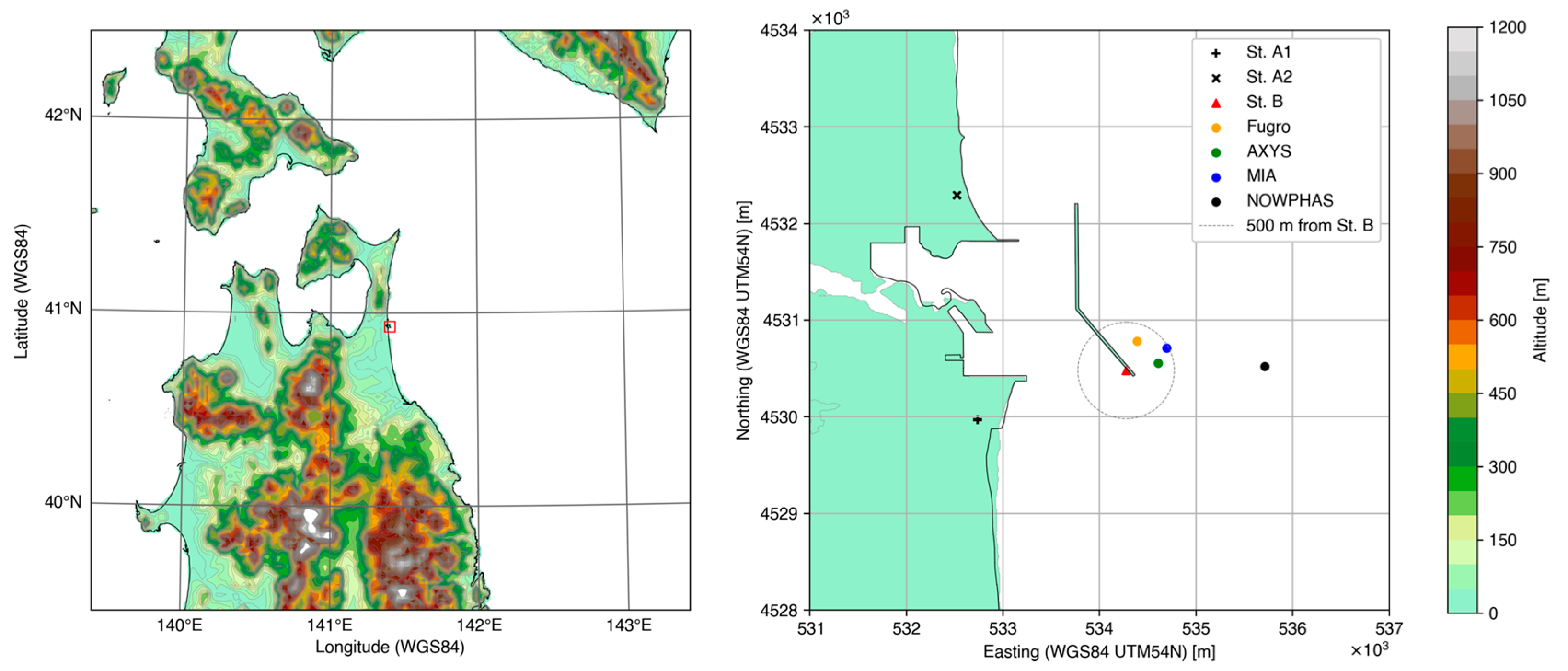
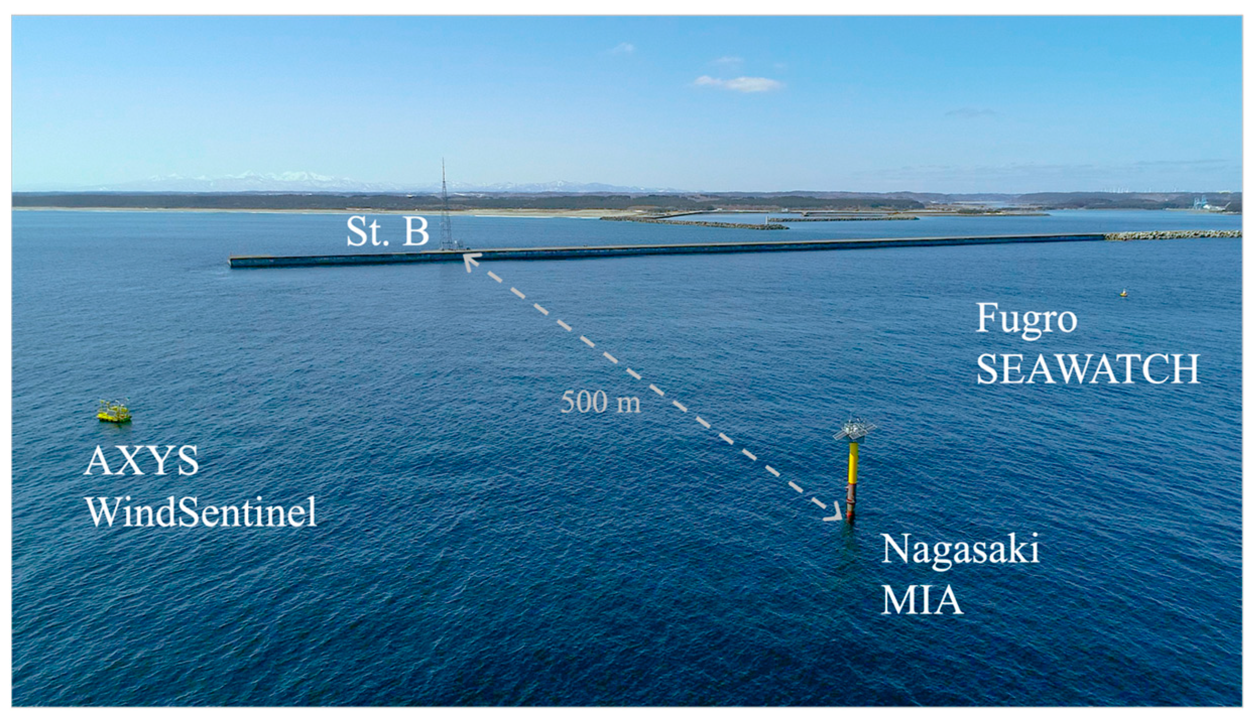
We use the same datasets employed in our previous study [10]. The Mutsu-Ogawara Port observatory site is located on the east coast of Aomori Prefecture, in the northeastern part of Japan, facing the Pacific Ocean. There is an offshore measurement station, St. B, on a breakwater approximately 1.5 km from the coastline, as well as the onshore stations, St. A1 and St. A2. Three FLSs are deployed within 500 m from St. B. The measurements are compared against the measurements taken at St. B. In addition, an ultrasonic wave height meter (Nationwide Ocean Wave Information Network for Ports and Harbors (NOWPHAS)) is installed at 1.5 km offshore from St. B [16]. The NOWPHAS data are used as a reference for ambient wave height and period measurements. Figure 1 presents the locations of the Mutsu-Ogawara site and measurement facilities, while Figure 2 shows an aerial photograph.

2.2. St. B Reference Vertical LiDAR on the Breakwater

As shown in Figure 3, a fixed VL and metmast are installed on the breakwater in St. B. To verify the motion-induced error in the standard deviation of wind speed and TI measurements by FLSs, Windcube V2.1, a pulsed VL installed on the fixed observation platform is mainly used for reference wind data. The fixed VL is configured to measure wind speed (10 min average and standard deviation) and wind direction (10 min average) up to 250 m above the mean sea level (AMSL), including several predefined representative heights (63, 120, and 180 m). For convenience, all measurement heights are represented as AMSL in this study unless otherwise specified.

Table 1. Configuration of the VL at St. B. Adapted and modified from [10].

Period	From 11 December 2020 to 23 November 2021
Location	On the observation platform next to the St. B metmast
LiDAR type	Windcube V2.1 (Vaisala (Vantaa, Finland), formerly Leosphere)
Measurement heights	50, 59, 63, 66, 80, 100, 120, 140, 160, 180, 200, and 250 m
Measurement parameters	10 min averaged wind speed and direction, standard deviation of wind speed, and TI at 63 m

shows the configuration of the fixed VL. The verification is carried out using approximately one year of data, from 11 December 2020 to 23 November 2021. The data availability of the fixed VL has been confirmed to be above 90%.

As site-specific conditions, we observed a speed-up effect of approximately 3% due to roughness change [17] and wave reduction owing to the breakwater when wind blows from onshore to offshore. Ideally, these need to be removed from the validation, as these local effects are absent in the site of interest where the FLS is deployed. Therefore, the verification of the FLS-measured standard deviation and TI is carried out only for timestamps when the wind direction is in a range of 0° to 180° (sea sector).

2.3. Reference Wave Data

As shown in Figure 1, a NOWPHAS sensor is installed at approximately 3 km from the coastline. The instrument is a seabed-installed wave height gauge that uses ultrasonic waves to capture sea-surface fluctuations. Using the zero-up crossing method, the NOWPHAS sensor calculates the significant wave height $H_{1/3}$ and period $T_{1/3}$, which represent the average of the highest one-third of the wave heights and its corresponding wave period, respectively.

2.4. Floating LiDAR System

Table 2. Specifications of the FLSs. Adapted and modified from [10].

	SEAWATCH	WindSentinel	MIA
Image
Manufacturer	Fugro	AXYS Technologies	Nagasaki 5 companies
Shape	Round	Ship	Spar
Dimensions	Height: 7.2 m Diameter: Ø 2.8 m	Height: 9 m Length: 6 m Width: 3.1 m	Height: 26 m Diameter: Ø 1.0 m (above water level), Ø 2.15 m (below water level) Maximum platform width: 5.5 m
Weight	Approximately 2.2 tons	Approximately 9 tons	Approximately 46 tons Platform: 2 tons Floater: 44 tons
Draft	Approximately 3 m	Approximately 2 m	Approximately 14.5 m
Material	Polyethylene, aluminum, and copper	Aluminum and copper	Copper and concrete
Mooring	Single-point catenary with a mid-float	Single-point catenary	Three-point catenary
Drifting radius	Approximately 100 m	Approximately 120 m	Approximately 20 m
Mooring chain length	Approximately 85 m	Approximately 120 m	Approximately 320 m × 3 chains
LiDAR(s)	FZX: ZX300M (ZX Lidars)	AZX: ZX300M (ZX Lidars) AWC: Windcube (Vaisala)	MDB: DIABREZZA (Mitsubishi Electric)
Analyzed data	.ZPH	AZX: .ZPH AWC: .sta	.csv
Power	Fuel cell, photovoltaic (PV), and battery	Wind turbine, PV, battery, and diesel generator	Fuel cell, PV, and battery
Meteorological parameters	Wind, temperature, and humidity	Wind, temperature, humidity, pressure, precipitation, and irradiance	Wind, temperature, humidity, and irradiance
Ocean parameters	Sea temperature, wave, and current	Sea temperature, wave, and current	Sea temperature

summarizes the three FLSs used in this study. The measurement campaign consists of two stage-3 commercial FLSs according to the OWA roadmap, and one FLS manufactured domestically in Japan. The SEAWATCH Wind LiDAR Buoy manufactured by Fugro (Leidschendam, The Netherlands) is a round-shaped buoy with a single-point mooring and is equipped with a ZX300M by ZX Lidars (Malvern, UK), a continuous-wave Doppler LiDAR (denoted as FZX). WindSentinel, manufactured by AXYS Technologies (Sidney, BC, Canada), is a ship-shaped buoy with a single-point mooring, like the Fugro SEAWATCH, but is equipped with two types of LiDAR, ZX300M and Windcube (WSL866), a pulsed Doppler LiDAR, denoted as AZX and AWC, respectively. We basically treat the two datasets as independent. The Marine Environmental Data Integrated Acquisition platform (MIA), jointly manufactured by five companies in Nagasaki Prefecture, Japan, is a spar-type buoy with three-point moorings; it is considered to have low motion owing to its structural stability. It is equipped with a DIABREZZA machine, a pulsed Doppler LiDAR by Mitsubishi Electric (Tokyo, Japan) that is similar to Windcube, on the upper deck of the buoy (MDB).

Although some of the systems have an FLS-specific algorithm to derive 10 min wind speed and its standard deviation from the raw measurements, and thus have different formats, we use only LiDAR native non-motion-compensated data to equivalently discuss the impact of the buoy’s motion on the measurement of the VL mounted on it. Therefore, for example, ZX’s native data are used for both FZX and AZX. All VLs on the FLSs are configured to cover the predefined representative heights, 63, 120, and 180 m.

We also analyze the buoys’ motion based on a gyro sensor mounted on each FLS. For SEAWATCH and MIA, the gyro sensor is integrated with the buoy system. For WindSentinel, the gyro sensor integrated with Windcube VL is analyzed. All raw data are resampled to 1 Hz, which is their lowest temporal resolution.

The campaign was conducted for 12 months starting from 24 November 2020 up to 23 November 2021. However, the period for FZX is limited only up to the end of August 2021 due to a wash-out event. The system and data availabilities have been discussed previously [10].

2.5. Turbulence Intensity

The study assesses the FLS-measured TIs, which are defined as the binned mean and 90 percentile values (TI_mean and TI_90%, respectively). These values are calculated as follows:

$${TI}_{mean}={\displaystyle \frac{{\overline{\sigma }}_k}{{\overline{u}}_k}},$$

(1)

$${TI}_{90\%}={\displaystyle \frac{{\overline{\sigma }}_k+1.28{\sigma }_{\sigma k}}{{\overline{u}}_k}},$$

(2)

where ${\overline{u}}_k$ is the binned wind speed in a width of 1 m/s, ${\overline{\sigma }}_k$ is the averaged standard deviation, and ${\sigma }_{\sigma k}$ is the standard deviation of the standard deviation in the wind speed bin $k$.

2.6. Quantification of the Buoy Motion

The FLS’s accuracy is considered to be sensitive to the buoy’s motion. Therefore, characterization of the buoy’s motion is essential. To quantify the motion, the buoy’s tilt ${\theta }_{\alpha }$ is analyzed at each time step, as in Equation (3), using the roll ${\theta }_r$ and pitch ${\theta }_p$ recorded using a gyro sensor on the buoy, as follows:

$${\theta }_{\alpha }={\cos }^{-1}\left(\cos {\theta }_r\cos {\theta }_p\right).$$

(3)

Further, significant tilt ${\theta }_{\alpha ,1/3}$ is defined, as in Equation (4), in a similar manner to that for the significant wave height, which is calculated as the average of the highest one-third of the wave heights collected within the averaging window, as follows:

$${\theta }_{\alpha ,1/3}={\displaystyle \frac{1}{\frac{1}{3}N}}\sum _{m=1}^{{\displaystyle \frac{1}{3}}N}{\theta }_{\alpha ,m},$$

(4)

where N is the number of peaks within the window, set as 10 min, and ${\theta }_{\alpha ,m}$ are the individual maximal values of the buoy tilt sorted in descending order. Thus, ${\theta }_{\alpha ,1/3}$ is a quantitative parameter reflecting the level of the buoy’s motion and is analyzed together with the peak period of the roll and pitch angles of the buoy. As an example, Figure 4 shows a time series of the roll ${\theta }_r$, pitch ${\theta }_p$, and tilt ${\theta }_{\alpha }$, and the calculated ${\theta }_{\alpha ,1/3}$ within an arbitrary 10 min for the Fugro SEAWATCH buoy.

2.7. Empirical Motion Correction

An empirical motion correction proposed in this paper is based on findings presented in Section 3. The standard deviation of wind speed observed by the FLS at every 10 min timestamp is reduced by the expected error, which is empirically obtained as a function of the significant tilt ${\theta }_{\alpha ,1/3}$ as follows:

$${\sigma }_{FLS,cor}=\max \left({\sigma }_{FLS}-f\left({\theta }_{\alpha ,1/3}\right),0\right),$$

(5)

where ${\sigma }_{FLS,cor}$ and ${\sigma }_{FLS}$ are corrected and raw standard deviations of wind speed, respectively, and $f\left({\theta }_{\alpha ,1/3}\right)$ is the obtained first-degree polynomial correction function that quantifies the error in standard deviation, as follows:

$$f\left({\theta }_{\alpha ,1/3}\right)=a\left\{1-\cos \left({\theta }_{\alpha ,1/3}\right)\right\}+b.$$

(6)

The slope $a$ and intercept $b$ for each FLS are discussed in Section 3. It is worth noting that motion, i.e., significant tilt ${\theta }_{\alpha ,1/3}$ is translated to $1-\cos \left({\theta }_{\alpha ,1/3}\right)$ because we found a better fitting in the regression line and, consequently, a better performance in the correction. Its physical meaning is the relative difference in the target height of the VL when the buoy experiences the tilt angle, as shown in Figure 5. For example, for the target at 63 m with the VL tilted by 15°, the VL ends up measuring at an approximately 3.4% lower height with respect to the center of the measuring cone.

3. Results

3.1. Analysis of the Buoys’ Motion

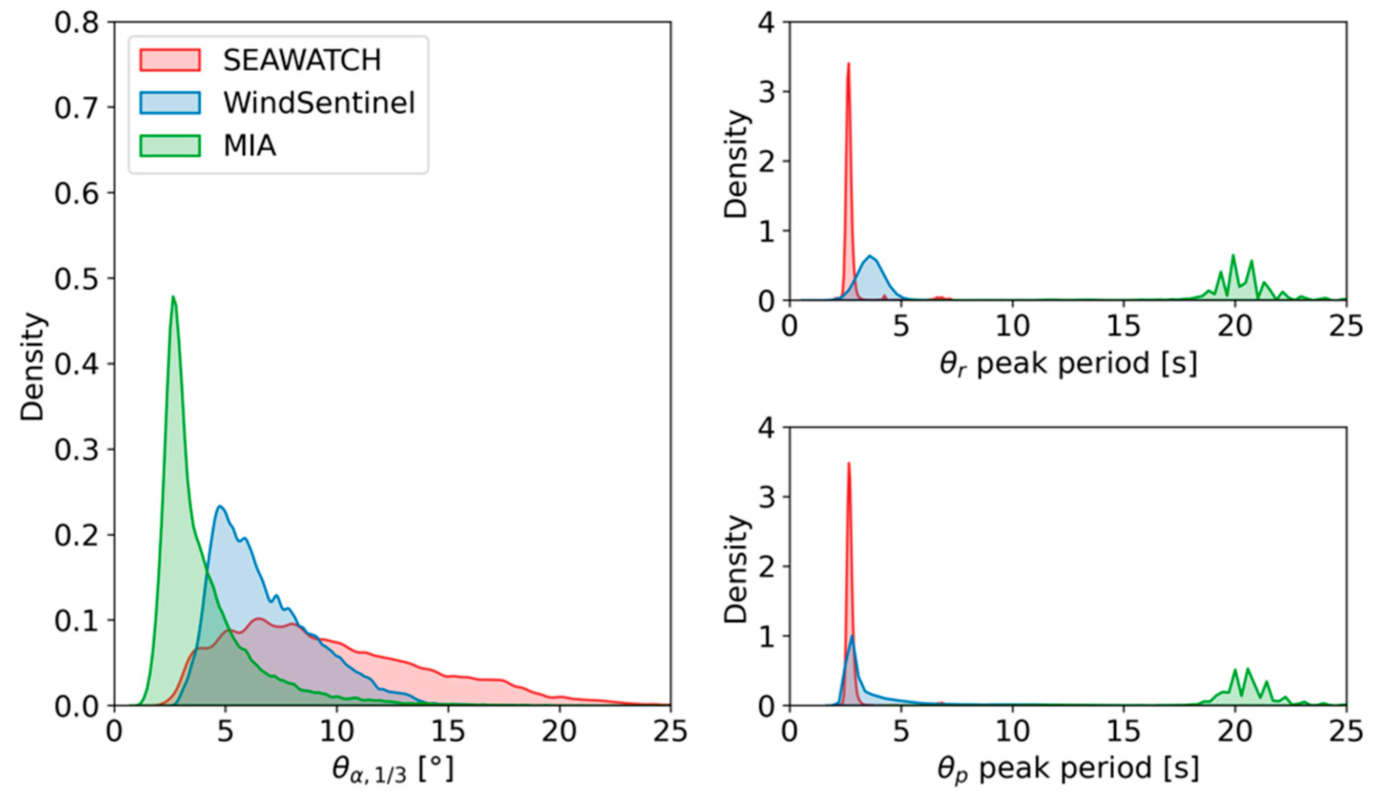
Figure 6 shows the significant tilt ${\theta }_{\alpha ,1/3}$ and peak periods of the roll ${\theta }_r$ and pitch ${\theta }_p$ for the three buoys. Notably, the motion of the buoy differs widely depending on its shape and mooring type. According to the significant tilt, SEAWATCH exhibits the largest motion and spread, MIA exhibits the smallest, and those of WindSentinel are in between. The spread, particularly for SEAWATCH and WindSentinel, seems to be affected by variable metocean conditions, while MIA exhibits a lower sensitivity. For the peak period, SEAWATCH and WindSentinel have smaller values (up to 5 s), while MIA exhibits a different distribution having a peak of around 20 s. WindSentinel has different peak periods for the roll and pitch, probably due to its anisotropic shape. However, compared to the distributions of the significant tilt, none are widely distributed. This suggests that, in general, the motion period of the FLS buoy does not change largely under variable metocean conditions and may be determined by the shape and mooring design. Regarding the sensitivity assessment of measurement error in the turbulent component, the focus should be on the significant tilt rather than on the motion period because the wave height affects the accuracy of the turbulence measurement of the FLSs [10]. According to this analysis, the MIA buoy is significantly stable, owing to its spar shape, compared to SEAWATCH and WindSentinel.

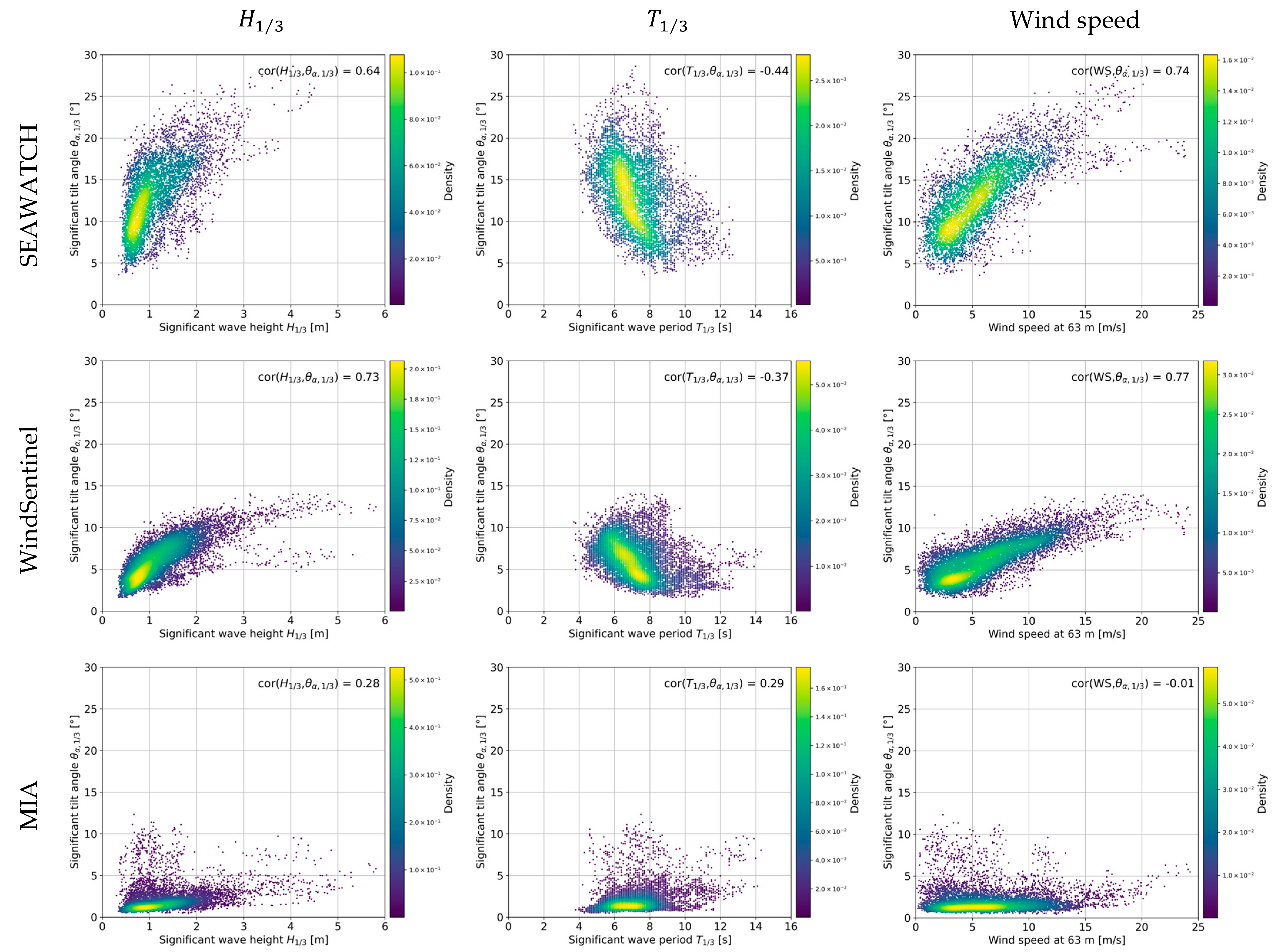
The sensitivity of the significant tilt angle ${\theta }_{\alpha ,1/3}$ to the wave and wind conditions is further analyzed. Figure 7 shows scatter plots of ${\theta }_{\alpha ,1/3}$ against the significant wave height $H_{1/3}$, wave period $T_{1/3}$, and wind speed. Regarding the wave height, all buoys exhibit positive correlations, suggesting that the buoy motion increases with the wave height, in general. SEAWATCH exhibits the most rapid increase in its ${\theta }_{\alpha ,1/3}$ with the wave height, followed by WindSentinel and MIA, which exhibits a low sensitivity. Regarding the wave period, negative correlations are observed for WAVEWATCH and WindSentinel, while that for MIA is positive because of the peak period of the buoy motion centered below 5 s for the first two buoys and 20 s for MIA, as shown in Figure 6. The sensitivity to wind speed exhibits a similar trend to that of the sensitivity to the wave height. MIA exhibits a low sensitivity for the wind speed below 15 m/s. However, the motion increases at higher wind speeds owing to the exposure to the high wind pressure. Overall, each buoy has different dimensions (weight, shape, and mooring), and thus different sensitivities of its motions to the environmental conditions. This is related to the motion-induced error in the measurement of turbulent components by FLS. On the other hand, ideally, the motion compensation should be universally applied to any type of FLS, regardless of the characteristics of the buoy. As the result shows the extent to which the significant tilt angle ${\theta }_{\alpha ,1/3}$ well represents both wind speed and wave height driven motions, it is expected to be effective for the assessment of the motion-induced error in the measurement of turbulent components.

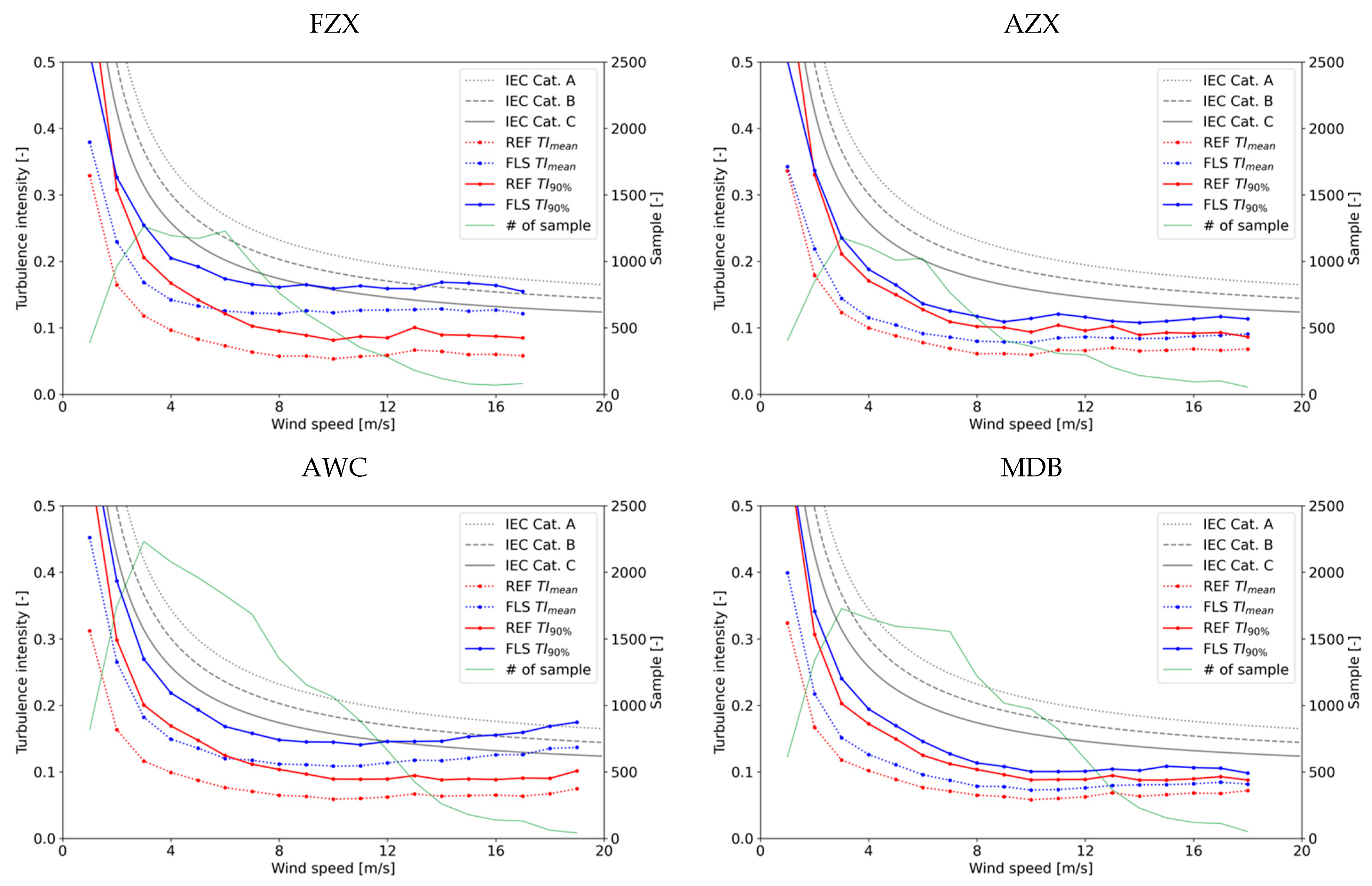
3.2. TI Without Motion Compensation

The performance of the FLS’s raw measurement for the turbulent component, without the use of a compensation algorithm, is analyzed with a comparison to a fixed VL. Figure 8 shows TI_mean and TI_90% as a function of the wind speed for both the FLS and fixed VL. The normal turbulence models (NTMs), categories A to C, as per IEC61400-1 [18], are also shown in Figure 8 as references. The overall result suggests that the FLS tends to overestimate both TI_mean and TI_90%. This trend is more notable for FZX and AWC than for AZX and MDB. It can easily be explained by comparing FLSs using the same LiDAR technology (FZX and AZX using a continuous-wave LiDAR and AWC and MDB using a pulsed LiDAR). If the same LiDAR technology is used, the FLS with a larger motion has a larger error in the turbulence measurement. Regarding the two measurements for AZX and AWC, which are installed on the same buoy and accordingly affected by the same motion, the pulsed-LiDAR may have a larger error. Finally, the differences between TI_mean and TI_90% for both fixed VL and FLSs are similar, which suggests that the standard deviation of the standard deviation in each wind speed bin (${\sigma }_{\sigma k}$) is relatively well captured, even by FLSs; however, the mean standard deviation (${\overline{\sigma }}_k$) is not well captured. Therefore, a correction for a systematic bias in TI is important for a better representation of both TI_mean and TI_90% by the FLS.

3.3. Relationship Between the TI Error and Buoy’s Motion

As suggested in the previous section, the error in standard deviation and TI is dependent on the buoy’s motion. To better understand this, a sensitivity assessment of the error to the buoy’s motions is qualitatively and quantitatively carried out. Figure 9 shows the relationship between the extent of motion in the x-axis and error in the standard deviation in the y-axis for wind speeds higher than 2 m/s. As previously mentioned in Section 2.7, the x-axis uses $1-\cos \left({\theta }_{\alpha ,1/3}\right)$ instead of ${\theta }_{\alpha ,1/3}$, because we found a clearer linear trend with this parameter. The range of the x-axis is 0 to 0.06 for FZX, AZX, and AWC and 0 to 0.01 for the MDB due to the smaller motion. To evaluate the systematic error, bin-averaged plots are also shown. Furthermore, the validity of the binned statistics is evaluated based on the number of samples, in accordance with the classification study in the IEC standard [19]. A linear regression is obtained for the valid bins that contain sufficient samples.

Overall, a clear positive relationship between the motion and error in standard deviation is observed for all units. The trend is well represented by the regression line, with R² higher than 0.98. In principle, the FLS predicts the fixed VL equivalent standard deviation and TI in the absence of motion. The regression line shows this as it approaches $y=0$ as x (motion of the buoy) decreases. Although there is still a small intercept in the case for MDB (0.076 m/s), it may be an error due to a constant tilt of the spar-type buoy, aside from the periodic motion. The slopes for those regression lines are divided into two groups. The FLSs with a continuous-wave LiDAR, i.e., FZX and AZX, have smaller slopes (13.8 and 12.8, respectively) than those with a pulsed LiDAR (34.5 for AWC and 28.3 for MDB), which suggests that the former FLSs are, in general, less sensitive to the motion in terms of the performances of the standard deviation and TI measurements. This probably occurs because the continuous-wave LiDAR requires only 1 s to obtain 50 Hz radial data and provides each wind vector, which is the basis of the 10 min wind speed and standard deviation, in the end, while the pulsed LiDAR needs approximately 4 s to obtain four radial wind speeds in all four directions and one vertical component. It is also worth mentioning that a side study with cup anemometers mounted on the collocated metmast shows a similar trend. Considering that the regression line well reflects the relationship between the overestimation of standard deviation by FLSs and buoy motion, it could be the basis of the motion compensation for a better representation of TI by FLSs.

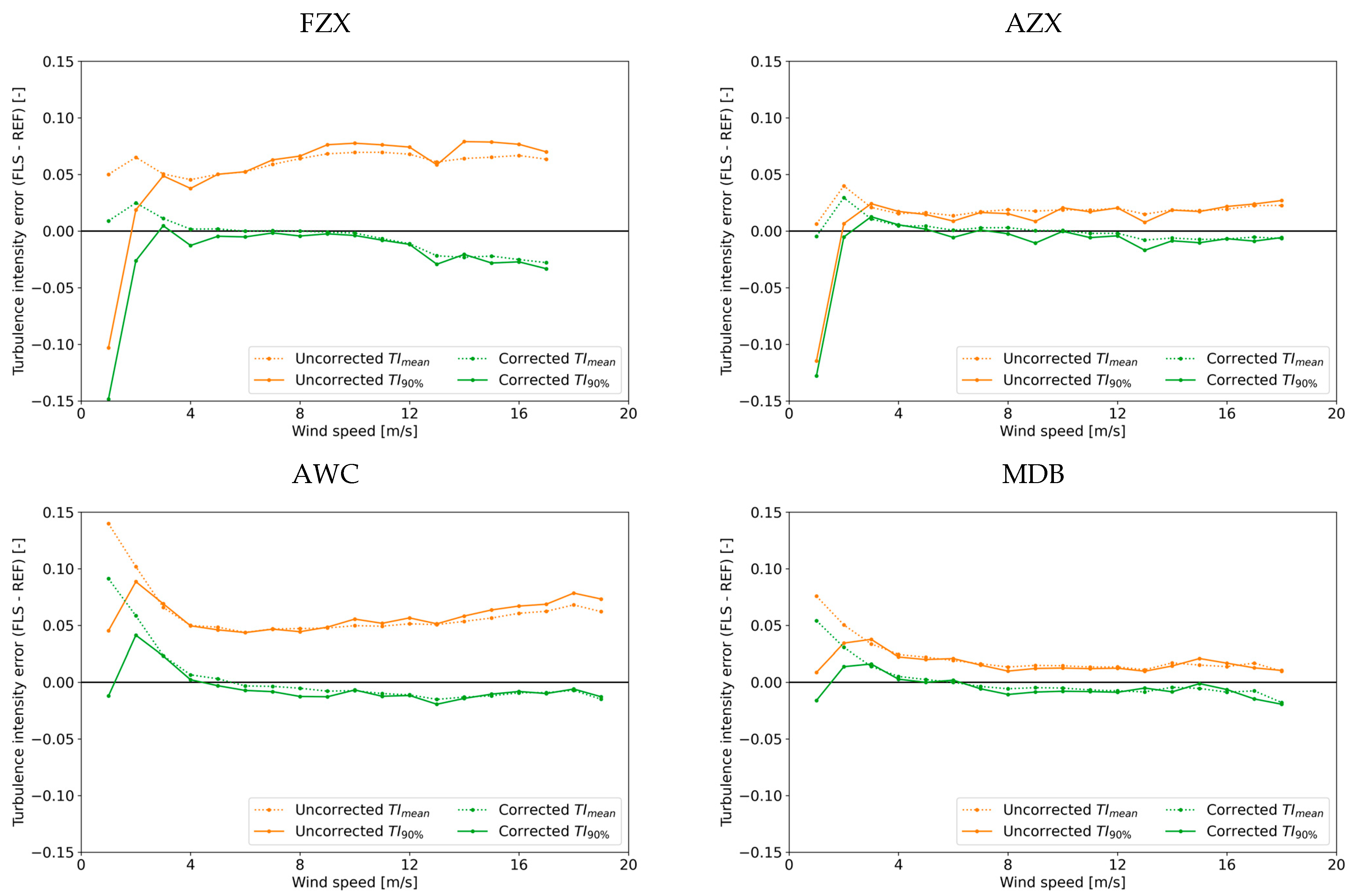
3.4. Correction of the FLS-Measured Standard Deviation Using an Empirical Regression Line

With the slope $a$ and offset $b$ obtained from the regression analysis in the previous section, the proposed correction method is applied to each FLS dataset in accordance with Equations (5) and (6). Figure 10 shows the resultant TI based on the corrected standard deviation of wind speed. Figure 11 shows the FLS TI estimation errors against the fixed VL before and after the correction is applied. Overall, these figures show a huge improvement in the FLS-measured TI_mean and TI_90% for all FLSs through the correction approach. Regarding the trend of the corrected TI, it may tend to be underestimated, i.e., overcorrected for a low wind speed, and vice versa for a high wind speed. The trend is observed for FZX and AWC. However, a large portion of the overestimation of TI by FLS is corrected by this approach. This implies that the motion of the FLS significantly contributes to the overestimated TI. Therefore, the assessment proves the benefit of the correction based on the single statistic parameter ${\theta }_{\alpha ,1/3}$, which represents the intensity of the buoy motion.

3.5. Dependence of the Correction Function on the Measurement Height

It is of significance to evaluate the change in the relationship between the error in the turbulence component and motion with the measurement height increase. The same analysis as that for Figure 9 in Section 3.3 was performed for 120 and 180 m. The obtained slope, offset, and R² are summarized in

Table 3. Slope, offset, and R² for the explanatory variable of $1-\cos \left({\theta }_{\alpha ,1/3}\right)$ and response variable of the error in standard deviation of wind speed ${\sigma }_{FLS}-{\sigma }_{REF}$ obtained by the sensitivity analysis, as in Figure 9, for the three representative measurement heights of 63, 120, and 180 m.

	63 m			120 m			180 m
	Slope a	Offset b	R2	Slope a	Offset b	R2	Slope a	Offset b	R2
FZX	13.775	−0.042	0.987	15.118	−0.053	0.989	15.394	−0.045	0.986
AZX	12.844	−0.015	0.991	13.312	−0.016	0.961	14.495	−0.023	0.950
AWC	34.520	−0.021	0.989	37.341	−0.032	0.986	38.315	−0.023	0.982
MDB	28.279	0.076	0.990	28.779	0.075	0.933	17.636	0.127	0.900

. For FZX, AZX, and AWC, the slope gradually increases with the measurement height but shows a constantly similar sensitivity. This implies that the impact of the buoy motion on the turbulence measurement tends to be more significant at larger measurement heights. This is in line with the common understanding that the swing of the measurement cone and, accordingly, the pointing error of LiDAR lead to a poorer measurement capability. For MDB, the slope rapidly dropped at 180 m, probably because the increased offset represents the largest error. As the range of the motion of MDB is considerably narrower than the others, the uncertainty in the determination of the slope and offset from the limited variability may be higher.

4. Discussion

This study was conducted with a focus on the performance of FLSs in TI measurements and the associated correction method using four FLS datasets on three different buoys at the Mutsu-Ogawara site in Japan. There are three key findings of this study with the use of the multiple FLSs. First, the error of the FLS’s TI measurement is largely affected by the buoy motion, and therefore by the buoy’s dimensions. Second, there is a similar relationship between the measurement error and buoy motion if the same VL type is used even on different buoys. This suggests that the development of a VL-specific motion compensation algorithm is possible. Third, the proposed correction algorithm based on the significant tilt angle ${\theta }_{\alpha ,1/3}$ has a good performance and significantly reduces the measurement error.

However, there are a few aspects to be discussed. The dataset used to understand the relationship between the error and buoy motion is the same as the dataset to which the correction is applied. Therefore, it is not surprising that a good performance of the correction is obtained. Nevertheless, it is still interesting to see how the “simplified” correction based only on the buoy motion ${\theta }_{\alpha ,1/3}$ can well remove the TI error. This demonstrates that the main source of the FLS TI error is the motion of the buoy, and that further development of the correction algorithm is possible. For example, there is a low sensitivity of the wind speed, aside from ${\theta }_{\alpha ,1/3}$ shown in Figure 9. It seems to account for the under- and overestimation of the TI at lower and higher wind speeds, respectively, observed for FZX and AWC in Figure 10 and Figure 11.

Further, the reference dataset used in this study is from a fixed VL, which also has a systematic error compared to a cup anemometer, as reported in our previous paper [10]. Thus, if the FLS TI is corrected by the algorithm proposed in this study, it is considered equivalent only to that of a fixed VL (more precisely Windcube V2.1) but not to that of a cup anemometer. In addition, if a different VL model, e.g., ZX300M, a continuous-wave VL, is used instead of Windcube as a reference fixed VL, different relationship and correction factors may be obtained. Furthermore, the dependence of the VL-measured TI on the measurement height is yet to be investigated. For FLSs, the amplified motion at larger measurement heights in addition to an increase in scan volume also needs to be investigated. These complexities should be addressed.

Despite the above limitations, the proposed motion compensation is rather simple to use and may be applied to any FLS dataset collected in the past by one of the VLs used in this study, as it requires only a gyro sensor to quantify the motion, without a physical upgrade to the FLS unit.

5. Conclusions

In this study, we investigated the performance of TI measurement by FLS and a motion compensation algorithm using four independent FLSs on three buoys with different motion characteristics. The obtained results can be summarized as follows.

The motion of the buoy and its response to environmental conditions, which are primarily wave height, period, and wind speed, are dependent on the shape and dimension of the buoy. A smaller buoy has a higher sensitivity to the wave, while a larger buoy has a low sensitivity. The significant tilt angle ${\theta }_{\alpha ,1/3}$ introduced in this study successfully quantifies the motion of the buoy regardless of the buoy’s shape and dimension.

The raw TI measurement by FLS has a poor accuracy against a fixed VL owing to the buoy motion causing the overestimation of TI. Particularly, for a smaller buoy (e.g., FZX), the magnitude of the overestimation is significantly larger than that on a larger buoy with less motion (i.e., MIA).

A clear correlation was obtained between the significant tilt angle ${\theta }_{\alpha ,1/3}$ and error in the standard deviation of wind speed, which suggests that the motion of the buoy has a primary role in the determination of the expected error of the turbulence measurement by FLS. Moreover, it was confirmed that if the VL is the same, there is a similar relationship between the tilt angle and error, even mounted on different buoys (e.g., FZX and AZX). This implies that the correction factor may be VL-specific regardless of the buoy on which the VL unit is mounted. The corrected TI is comparable to that of a fixed VL, which supports the above statements.

Further assessments shall be carried out to better understand the contribution of the measurement height and other environmental conditions to the error of the turbulence measurement by FLS. The ultimate goal is to obtain the correction factors that can be applied globally to any type of FLS.

References

- Gottschall, J.; Wolken-Möhlmann, G.; Viergutz, T.; Lange, B. Results and conclusions of a floating-lidar offshore test. Energy Procedia 2014, 53, 156–161. [Google Scholar] [CrossRef]
- Gottschall, J.; Gribben, B.; Stein, D.; Würth, I. Floating lidar as an advanced offshore wind speed measurement technique: Current technology status and gap analysis in regard to full maturity. WIREs Energy Environ. 2017, 6, e250. [Google Scholar] [CrossRef]
- Vepa, K.S.; Duffey, T.; Paepegem, W.V. Gyroscope-based floating lidar design proposal for getting stable offshore wind velocity profiles. Sea Technol. 2016, 57, 41–43. [Google Scholar]
- Bischoff, O.; Würth, I.; Gottschall, J.; Gribben, B.; Hughes, J.; Stein, D.; Verhoef, H. IEA Wind, Expert Group Report on Recommended Practices, 18. Floating LiDAR Systems, First Edition. 2017. Available online: https://iea-wind.org/wp-content/uploads/2020/12/IEA-Wind-RP-18-Floating-Lidar-Systems-fnl1.pdf (accessed on 31 March 2025).
- Mathisen, J.-P. Measurement of Wind Profile with a Buoy Mounted Lidar. 2013, p. 19. Available online: www.sintef.no/globalassets/project/deepwind-2013/deepwind-presentations-2013/c2/mathisen-j.p_fugro-oceanor.pdf (accessed on 31 March 2025).
- Bischoff, O.; Würth, I.; Cheng, P.; Tiana-Alsina, J.; Gutiérrez, M. Motion effects on lidar wind measurement data of the EOLOS buoy. In Proceedings of the First International Conference on Renewable Energies Offshore, Lisbon, Portugal, 24–26 November 2014. [Google Scholar]
- Bischoff, O.; Yu, W.; Gottschall, J.; Cheng, P.W. Validating a simulation environment for floating lidar systems. J. Phys. Conf. Ser. 2018, 1037, 052036. [Google Scholar] [CrossRef]
- Bastigkeit, I.; Leimeister, M.; Watson, W.; Wolken-Möhlmann, G.; Gottschall, J. Enhanced design basis for offshore wind farm load calculations based on met-ocean data from a floating lidar system. J. Phys. Conf. Ser. 2021, 2018, 012008. [Google Scholar] [CrossRef]
- Ohsawa, T.; Shimada, S.; Kogaki, T.; Iwashita, T.; Konagaya, M.; Araki, R.; Imamura, H. Progress of NEDO project “Bottom fixed offshore wind farm development support project (Establishment of offshore wind resource assessment method)”. Proc. Jpn. Wind Energy Symp. 2020, 42, 136–139. [Google Scholar]
- Uchiyama, S.; Ohsawa, T.; Asou, H.; Konagaya, M.; Misaki, T.; Araki, R.; Hamada, K. Accuracy Verification of Multiple Floating LiDARs at the Mutsu-Ogawara Site. Energies 2024, 17, 3164. [Google Scholar] [CrossRef]
- Carbon Trust Offshore Wind Accelerator (OWA). Roadmap for the Commercial Acceptance of Floating LIDAR technology. 2018. Available online: https://ctprodstorageaccountp.blob.core.windows.net/prod-drupal-files/documents/resource/public/Roadmap%20for%20Commercial%20Acceptance%20of%20Floating%20LiDAR%20REPORT.pdf (accessed on 31 March 2025).
- Thiébaut, M.; Thebault, N.; Le Boulluec, M.; Damblans, G.; Maisondieu, C.; Benzo, C.; Guinot, F. Experimental Evaluation of the Motion-Induced Effects for Turbulent Fluctuations Measurement on Floating Lidar Systems. Remote Sens. 2024, 16, 1337. [Google Scholar] [CrossRef]
- Kelberlau, F.; Neshaug, V.; Lonseth, L.; Bracchi, T.; Mann, J. Taking the motion out of floating lidar: Turbulence intensity estimates with a continuous-wave wind lidar. Remote Sens. 2020, 12, 898. [Google Scholar] [CrossRef]
- Kelberlau, F.; Neshaug, V.; Venu, A. Assessment of turbulence intensity estimates from floating lidar systems. J. Phys. Conf. Ser. 2023, 2507, 012014. [Google Scholar] [CrossRef]
- Rapisardi, G.; Araújo da Silva, M.P.; Miquel, A. A Machine Learning Approach to Correct Turbulence Intensity measured by Floating Lidars. J. Phys. Conf. Ser. 2024, 2767, 092050. [Google Scholar] [CrossRef]
- The Nationwide Ocean Wave Information Network for Ports and HArbourS (NOWPHAS). Available online: https://www.mlit.go.jp/kowan/nowphas/index_eng.html (accessed on 23 December 2024).
- Konagaya, M.; Ohsawa, T.; Inoue, T.; Mito, T.; Kato, H.; Kawamoto, K. Land–Sea Contrast of Nearshore Wind Conditions: Case Study in Mutsu-Ogawara. SOLA 2021, 17, 234–238. [Google Scholar] [CrossRef]
- IEC 61400-1; Ed. 4.0 Wind Energy Generation Systems—Part 1: Design Requirements. International Electrotechnical Commission: Geneva, Switzerland, 2019.
- IEC 61400-12-1; Ed. 2.0 Wind Energy Generation Systems—Part 12-1: Power Performance Measurements of Electricity Producing Wind Turbines. International Electrotechnical Commission: Geneva, Switzerland, 2017.