Melting in Shell-and-Tube and Shell-and-Coil Thermal Energy Storage: Analytical Correlation for Melting Fraction

Abstract

The following study investigated the melting behavior of coconut oil as a phase-change material in shell-and-tube and shell-and-coil thermal energy storage systems. The primary objective was to deepen the understanding of PCM melting dynamics under varying boundary conditions, aiming to optimize TES designs for renewable energy applications. This research addresses a gap in understanding how different heat-transfer configurations and boundary conditions affect melting efficiency. Experimental setups included two distinct heat-transfer surfaces in a cylindrical shell—a copper tube and a copper coil—tested under constant wall temperatures (34 °C for the tube, 33 °C for the coil) and constant heat flux (597 W/m² for the coil). Findings reveal that melting under constant heat flux takes approximately twice as long as under constant wall temperatures, underscoring the critical role of heat-transfer conditions in TES performance. The liquid fraction was estimated using two approaches: image-based analysis and the volume-averaged temperature method. The former proved less reliable due to geometric limitations, particularly when the heat-transfer surface was distant from the shell wall. Conversely, the latter yielded higher accuracy, especially in the shell-and-tube setup. Due to the scarcity of correlations for constant heat-flux conditions, the novel contribution of this work is the development of a modified semi-empirical correlation for the shell-and-coil TES system. For this purpose, an existing model, which demonstrated strong alignment with experimental data, was adapted. The findings suggest that slower melting under constant heat flux could benefit applications needing sustained heat release, like solar energy systems. Future work could investigate additional PCMs or novel geometries to further improve TES efficiency and scalability.

1. Introduction

Thermal energy storage (TES) systems are increasingly vital in addressing the dual challenges of rising energy consumption and environmental degradation. These systems enable the efficient storage and release of thermal energy, supporting the integration of renewable energy sources like solar [1,2], as well as the recovery of waste heat from industrial processes [3,4]. Among the various TES technologies, latent heat thermal energy storage (LHTES) utilizing phase-change materials (PCMs) stands out due to its high energy storage density and ability to maintain near-isothermal conditions during phase transitions. Organic PCMs, such as coconut oil, paraffin, and fatty acids, have attracted significant interest because of their recyclability, chemical stability, non-toxicity, and favorable thermophysical properties, positioning them as sustainable alternatives to synthetic materials [5,6,7].

The melting process of PCMs is a cornerstone of LHTES system performance, influencing both efficiency and practical applicability. Over time, research has focused on melting under constant wall-temperature boundary conditions (Dirichlet condition), or at least constant inlet temperatures, which simplifies analytical modeling and experimental design [8,9,10]. However, many real-world applications—such as solar thermal collectors, electronics cooling, nuclear reactor safety systems, and building HVAC systems—operate under constant heat-flux conditions, where heat input remains steady rather than temperature [11,12,13]. This mismatch between research focus and practical scenarios underscores the need for a deeper understanding of PCM melting dynamics under constant heat flux to optimize TES system design for diverse operational contexts [14,15].

A thorough review of the existing literature highlights a wealth of studies examining PCM melting under constant heat flux, particularly in rectangular geometries. For instance, M. Fadl and P. C. Eames [16] conducted experimental studies on RT44HC in a rectangular test cell, demonstrating a clear relationship between heat-flux magnitude and the evolution of the liquid fraction over time. Similarly, R. García-Roco et al. [17] explored the thermocapillary-driven melting of n-octadecane in a rectangular container under microgravity, emphasizing the critical role of natural convection in shaping melting behavior [18,19,20]. S. Huang et al. [21] investigated the influence of container height on RT42 melting under constant heat flux, revealing geometric effects on heat-transfer efficiency. Meanwhile, S. Motahar [11] leveraged artificial neural networks to predict melting patterns in rectangular enclosures, offering a computational approach to understanding complex, dynamic scenarios [20,22,23,24]. Collectively, these studies have elucidated key heat-transfer mechanisms, including the shift from conduction-dominated to convection-dominated regimes, and the impact of parameters such as heat-flux intensity, container aspect ratio, and PCM properties.

Beyond fundamental melting dynamics, researchers have also pursued strategies to enhance PCM performance under constant heat-flux conditions. N. S. Dhaidan et al. [12] examined the melting of nano-enhanced PCMs in a tube-in-tube configuration, finding that nanoparticle additives significantly boost thermal conductivity and reduce melting time. K. Chintakrinda et al. [13] compared enhancement techniques such as graphite nanofibers and metal foams in a heat sink, underscoring the importance of tailoring enhancement methods to specific applications like electronics cooling [25,26,27]. Y. Huo and Z. Rao [28] simulated PCM melting under constant heat flux, noting that while higher heat fluxes accelerate melting, they compromise the PCM’s ability to maintain stable temperatures during phase change. These advancements highlight the potential for material and system optimization, yet they also reveal gaps in applying such insights to non-rectangular geometries.

Despite the progress in rectangular systems, cylindrical TES configurations—particularly those with helical-coil heat exchangers—remain underexplored under constant heat-flux conditions. Cylindrical geometries are widely used in practical TES applications due to their compact design, structural integrity, and enhanced heat-transfer characteristics facilitated by curved surfaces and coil arrangements [29,30,31]. However, the complex interplay of geometry, boundary conditions, and fluid dynamics in these systems poses unique challenges. For example, M. H. Joneidi et al. [32] studied the effects of heat flux and tilt angle on PCM melting in a rectangular chamber, but their findings are not directly applicable to cylindrical setups with coils. V. Shatikian et al. [33] performed numerical analyses of PCM melting in a heat sink with vertical fins under constant heat flux, yet their focus on planar geometries limits its relevance to cylindrical systems. This research gap motivates a targeted investigation into cylindrical TES systems with coil configurations, which is a continuation of the author’s previous studies in this field [30,31,34,35,36].

One of the key factors for analyzing the melting process is the amount of liquid fraction; it can be treated as a thermal state of charge in TES applications. There are a few methods known from the literature used to obtain the dynamic of the melting phase: the use of thermochromic liquid crystals [37], ultrasonic methods [24], image data analysis [34], temperature field analysis (also called the interpolation method or volume-averaged temperature analysis [38]), and X-ray computed tomography [39].

The space between the coil and the shell is filled with coconut oil. It was chosen due to being non-toxic, abundant in nature, affordable, and readily available commercially. What is more, it can be seen as a good alternative to artificially produced PCMs, due to problems with their later utilization. Additionally, coconut oil has relatively favorable thermophysical properties, such as thermal conductivity greater than 0.3 W/mK. The thermophysical properties of coconut oil used for the calculations are shown in

Table 1. Thermophysical properties of coconut oil.

Property	Value	Unit
$\lambda$	0.329	W/mK
$\mathsf{\rho }$	1130	Kg/m3
$h$	146.7	kJ/kg
$c_p$	2.07	kJ/kg·K
$T_m$	25.5	°C
$\mu$	0.02	Pa·s
$\nu$	1.77 × 10−5	m2/s
$\mathsf{\beta }$	7.61 × 10−4	1/K
$\mathsf{\alpha }$	1.4 × 10−7	m2/s
$Pr$	125.8	-

. The coil was heated with a constant heat flux obtained through a DC power supply.

A key contribution of this study is the development of a modified analytical correlation for predicting the liquid fraction, adaptable to both constant wall-temperature and constant heat-flux conditions. As shown in

Table 2. Various correlations for the liquid fraction from the literature.

Year	Article	Correlation	Boundary Condition	PCM
1986	[42]	$\mathsf{\phi }=6.278{{\tau }_l}^{0.842}{{Ste}_l}^{0.0393}{A}^{0.0137}$	$T_w=const$	gallium (pure)
1993	[18]	$\mathsf{\phi }=0.2(1-1.35ln{S}_c)Ste{Fo}^{*}$	$q=const$	n-Octadecane (pure)
1999	[43]	$\mathsf{\phi }=4.73{Fo}^{0.906}{Ste}^{1.538}{Ra}^{0.002}$	$q=const$	PEG900
2001	[19]	$\mathsf{\phi }=1.43(0.957-e^{{\displaystyle \frac{4865SteFo}{{Ra}^{\raisebox{1ex}{$1$}\!\left/ \!\raisebox{-1ex}{$5$}\right.}}}})$	$q=const$	gallium (pure) n-Eicosane (pure) n-Tricontane (pure)
2018	[44]	$\mathsf{\phi }=0.596X+0.0438X^2-0.0825X^3+0.0130X^4$	$T_w=const$	Li2CO3–K2CO3
2019	[45]	$\mathsf{\phi }={\left[{\displaystyle \frac{0.1Fo{Re}^{0.064}{Ra}^a{Ste}^{*1.206}{\phi }^{0.0106}\left(21.178\sigma +\frac{0.1}{\sigma }\right)}{{\left(L/D\right)}^{0.3795}}}\right]}^{0.7}$	$T_w=const$	lauric acid (pure)
2023	[41]	$\mathsf{\phi }={\displaystyle \frac{C{Ste}^A{Ra}^B{Re}^D{Fo}^E}{{\left(L/D\right)}^F}}$	$T_w=const$	RT35

, correlations for constant heat flux lag behind those for constant temperature, hindered by the complexity of cylindrical systems and the rise of CFD studies, which is evidenced by the author’s recent review study [40]. Building on models like L.S. Raj et al. [41], this correlation incorporates geometric factors (e.g., coil diameter, cylinder radius) and dimensionless numbers (e.g., Stefan, Fourier), validated against experimental data to provide a versatile tool for TES design. The semi-empirical model can then be integrated into larger system models (e.g., solar thermal collectors, building heating systems, etc.) using connectors and standardized interfaces.

As shown before, the existing research on PCM melting under constant heat flux primarily focuses on rectangular TES systems, often comparing experimental and numerical results. However, these geometries, including flat walls and shell-and-tube configurations, are suboptimal for TES systems due to inefficient heat-transfer surface arrangements. This study addresses this gap by investigating a cylindrical TES system with a helical coil, filled with coconut oil, to enhance melting and solidification efficiency. It introduces a novel approach for practical applications, such as domestic hot water systems, district heating, and waste heat storage. Two distinctive methods were used to estimate the liquid fraction: an image-based technique, limited by the coil’s positioning obstructing melt front visualization, and a robust temperature-based method using thermocouple data, consistent with prior shell-and-tube studies.

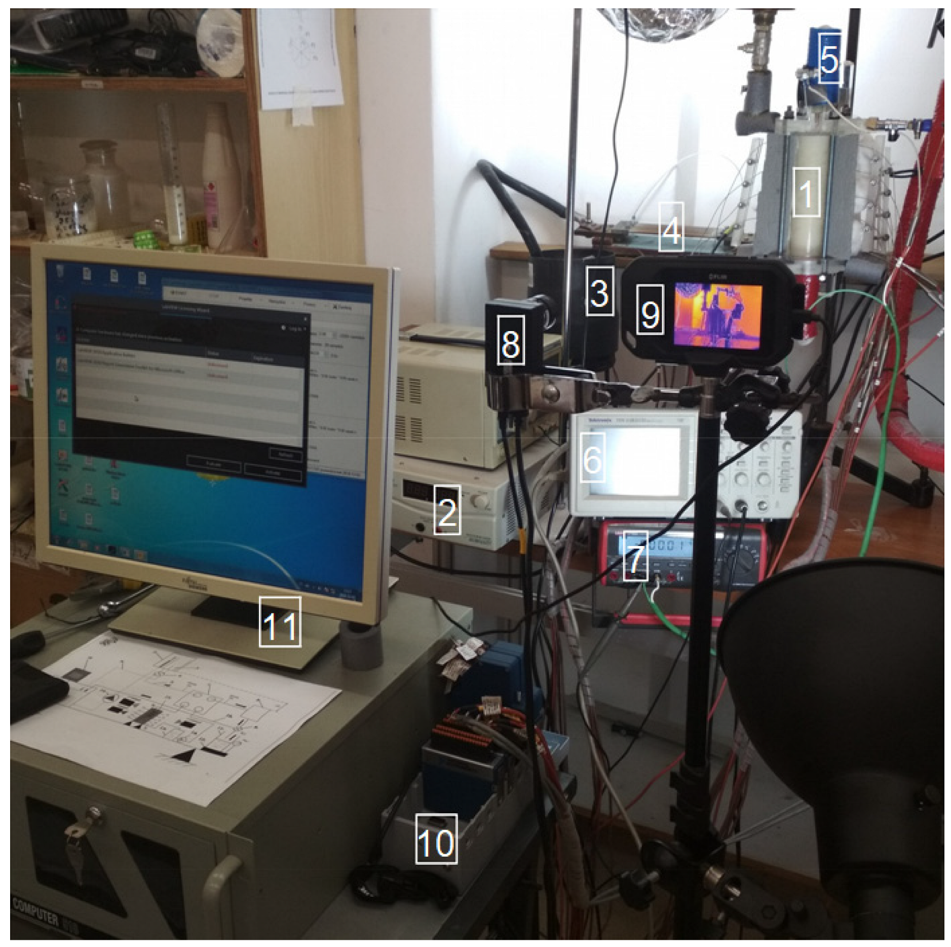
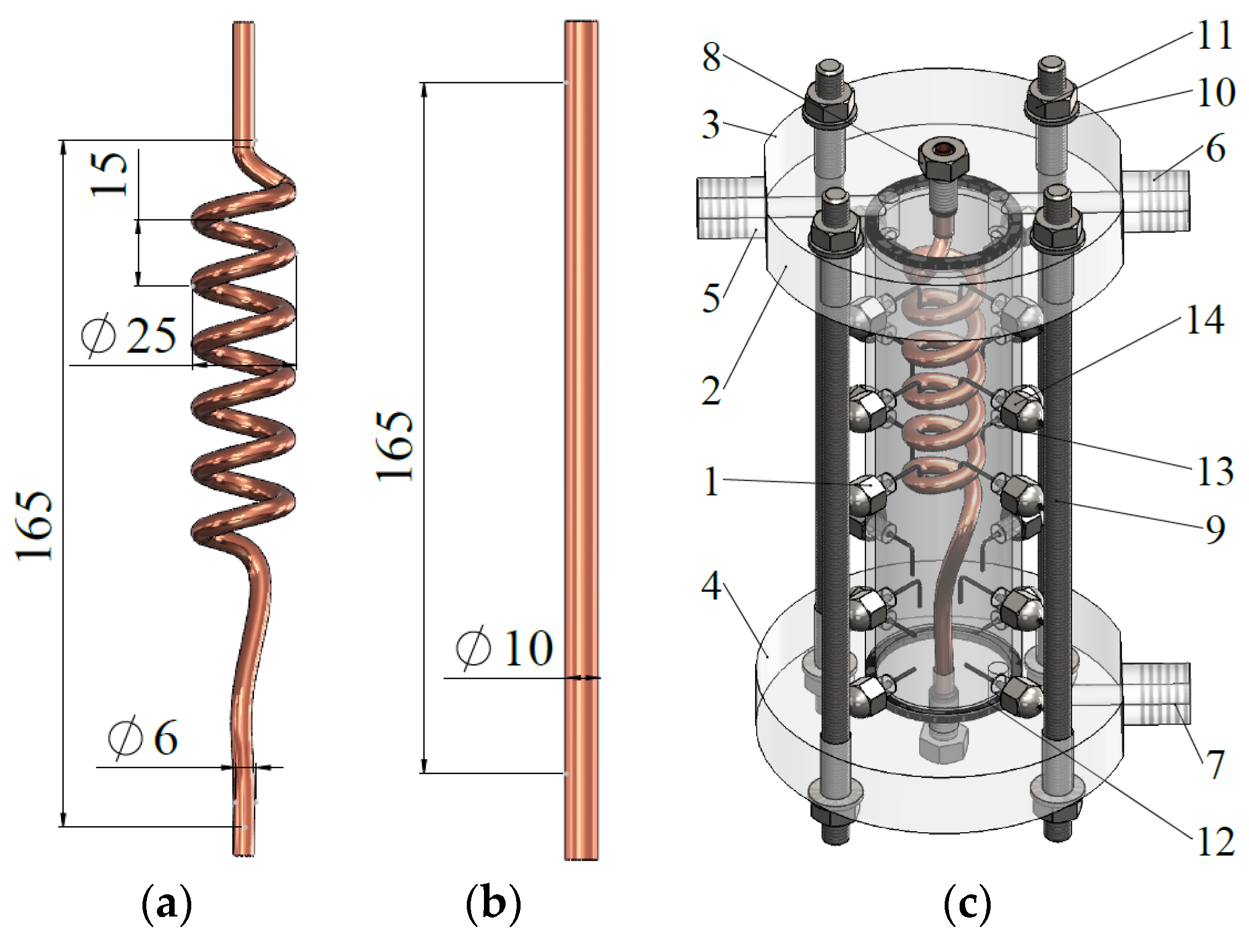
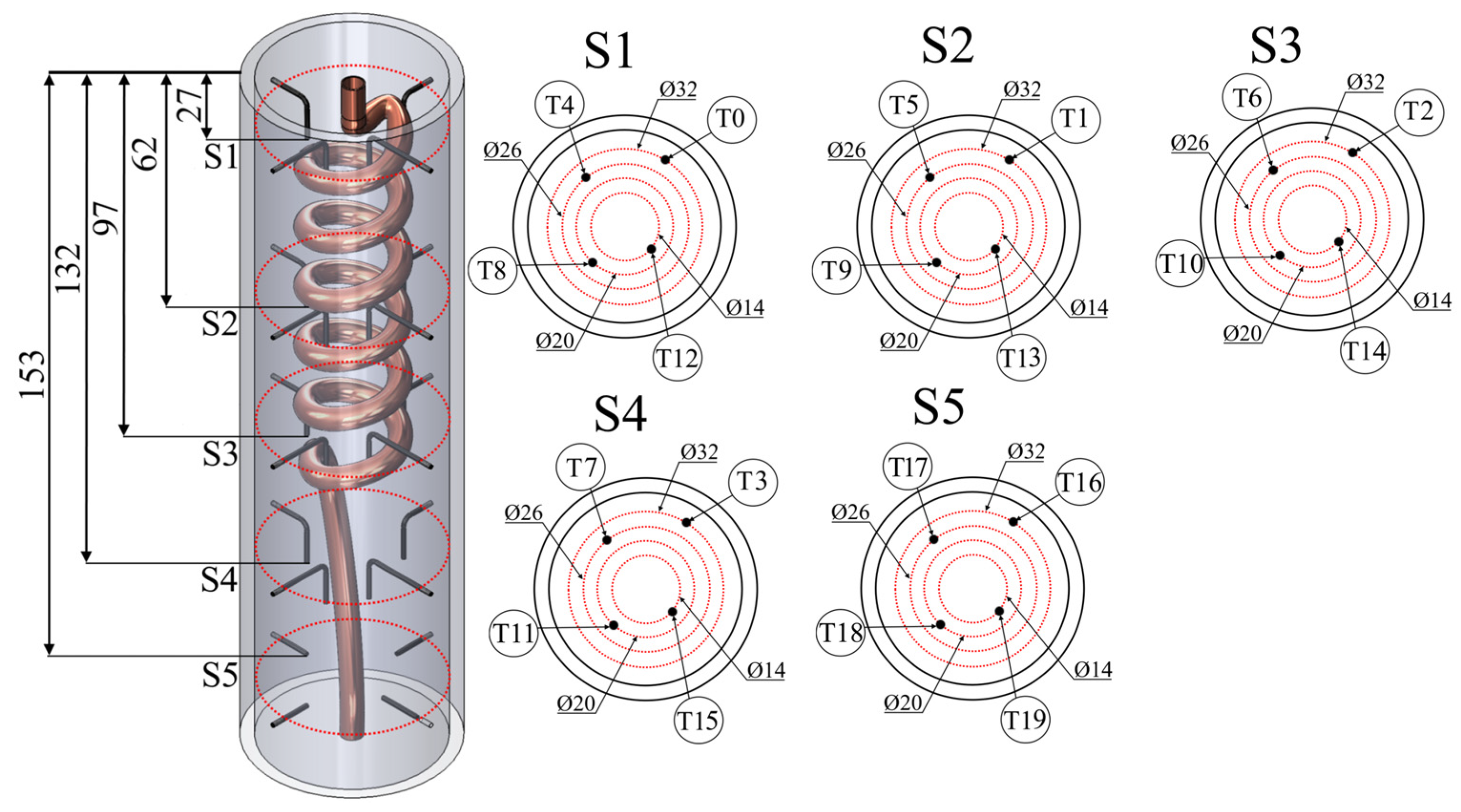
2. Materials and Methods

The schematic diagram of the experimental setup is shown in Figure 1. The copper heating element, in the form of a helical coil tube or a straight tube, was placed along the shell of TES system (1) and was connected to a SPS9600 MANSON DC power supply (2) to ensure a constant heat flux. Due to the low electrical resistivity of the heating material, the power supply loop was equipped with an additional load circuit (3) to maintain stable operation. Accurate determination of the supply current was achieved by measuring the voltage drop across a set of MERA LUMEL shunt resistors (4). Both shunts and the ends of a heating element were connected to a TDS210 TEKTRONIX oscilloscope (5). As part of the control procedures, a UT804 UNI-T multimeter (6) was used to independently verify the electrical parameters. Individually calibrated T-type thermocouples were connected to the data acquisition system (7). An HD UI1220ME-C-HQ high-speed camera (8) with a resolution of 752 × 480 pixels was used to record the melting process, capturing images at a frequency of 2 Hz (every 0.5 s). Both the data acquisition system and the camera were integrated with the PC station (9), allowing for simultaneous data logging of temperature and images. This solution eliminated the risk of time shifts. The calibration of the experimental setup is described in more detail in the authors’ previous study [35].

A photograph of the experimental stand is presented in Figure 2.

Figure 3 shows the design diagram of the TES system. The cylindrical shell (1) with an internal diameter of 40 mm was made of transparent acrylic glass, allowing for the observation of the PCM melting process. The heating element (2) was placed inside the shell and took the geometry of a helical coil (Figure 3a) or a straight pipe (Figure 3); it was made of a copper tube with a wall thickness of 0.5 mm. Regardless of the adopted configuration, the heat-transfer surface remained the same—around 8670 mm². The shell was closed from the top and bottom flanges (3 and 4), also made of acrylic. The flanges contained nozzles that allow the system to be operated during the preparation of the experiment. Additionally, central nozzles (8) were placed in the geometric centers of both flanges, the task of which was to stabilize the position of the heating element. The flanges and the shell were connected using four threaded rods (9). To ensure full tightness, silicone seals (12) were placed in the flange grooves. Dedicated connectors (14) were used to mount thermocouples (13), enabling their stable placement in the shell.

Uncertainties of all measured parameters are shown in

Table 3. Uncertainties of measured parameters.

Parameter	Units	Operating Range	Uncertainty	Error
$T$	°C	10–60	±0.2	-
$U$	V	1	±2 × 10−3	-
$I$	A	5.13	±0.01	-
$\dot{Q}$	W	50	±0.02	-
$L$	m	0.46	±5 × 10−4	-
$d_{out}$	m	6 × 10−3	±4 × 10−6 [46]	-
A	m2	8.67 × 10−3	7.23 × 10−4	±8%
$q$	W/m2	597	±4	±0.8%

.

Heat flux $q$ in this study is calculated as follows:

$$q={\displaystyle \frac{UI}{\pi d_{out}L}}$$

(1)

For calculating the heat-flux uncertainty $∆q$, a method of propagation of uncertainty is used [47], as presented below:

$$∆q=\sqrt{{\left({\displaystyle \frac{\partial \mathrm{q}}{\partial \mathrm{U}}}∆U\right)}^2+{\left({\displaystyle \frac{\partial \mathrm{q}}{\partial \mathrm{I}}}∆I\right)}^2+{\left({\displaystyle \frac{\partial \mathrm{q}}{\partial d_{out}}}∆d_{out}\right)}^2+{\left({\displaystyle \frac{\partial \mathrm{q}}{\partial \mathrm{L}}}∆L\right)}^2}$$

(2)

The heat-flux measurement uncertainty was about ±4 W/m², which produces an error of about ±0.8%. Similar calculations were carried out for the heat-transfer surface, and the results indicated a measurement uncertainty of about ±8.67 × 10⁻³ m², which produces an error of ±8%. To obtain the PCM temperature distribution, 20 individually calibrated thermocouples with an accuracy of 0.2 °C were used. All thermocouples, regardless of the coil used, were placed with four sensors on each of five surfaces (S1–S5). Detailed dimensions of the thermocouple arrangement are shown in Figure 4.

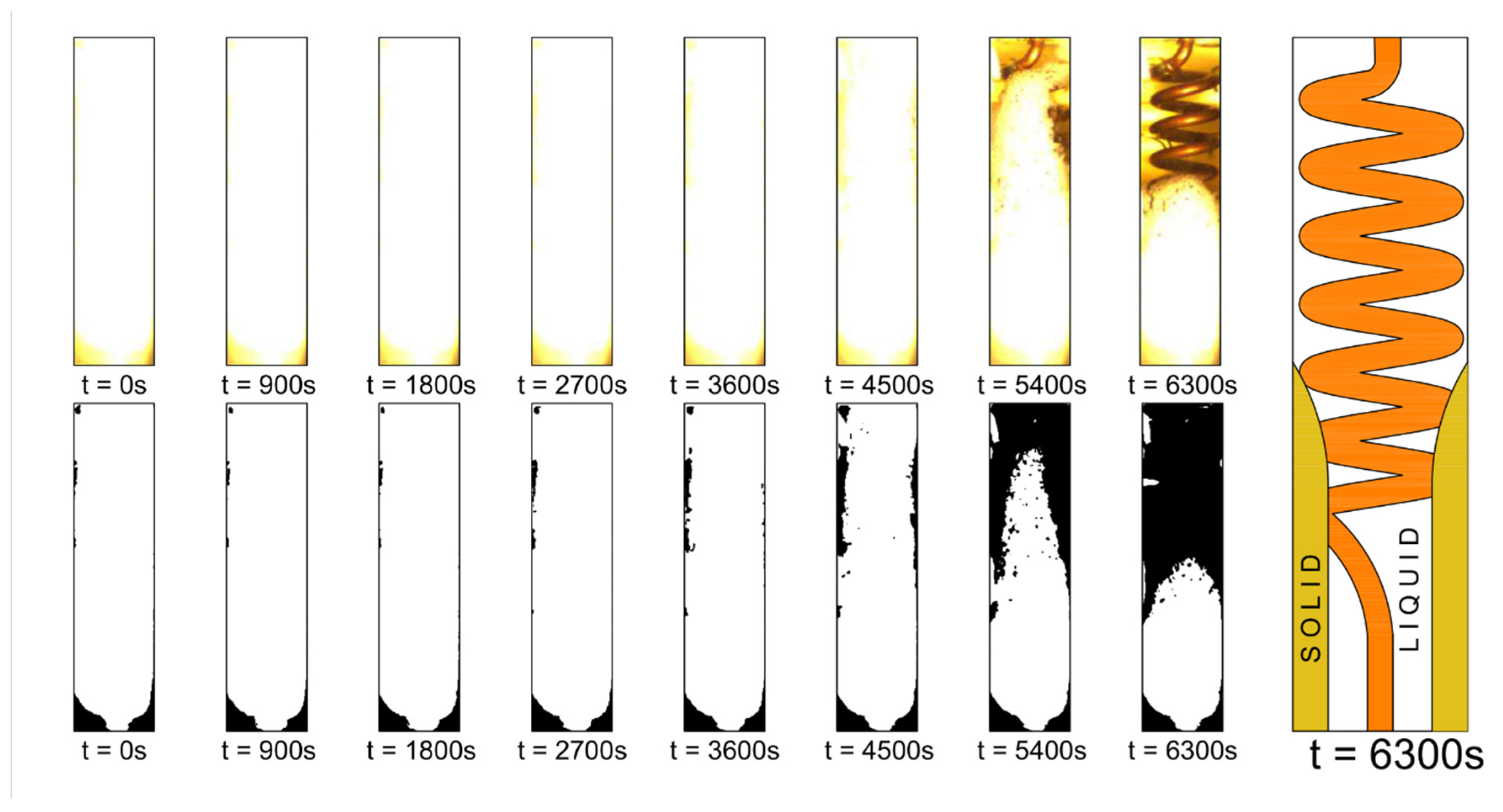
3. Visual Observations

High-resolution photographs of the thermal energy storage (TES) system were captured every 0.5 s to monitor the melting of coconut oil under three conditions: a tube at constant wall temperature ($T_w=34°\mathrm{C}$), a coil at constant wall temperature ($T_w=33°\mathrm{C}$), and a coil at constant heat flux ($q=597\mathrm{W}/{\mathrm{m}}^2$). Each image was processed through binarization to estimate the liquid fraction via a binary ratio—a method adapted from Boroojerdian et al. [48]. Figure 5 showcases various binarization techniques applied to images of the coil under constant heat flux, as explored in R. Petryniak [49]. These include simple binarization with thresholds of 100, 150, 200, and 250 (Figure 5a–e), and advanced algorithms, such as Otsu (Figure 5f), Savuola (Figure 5g), and Niblack (Figure 5h).

The Otsu algorithm determines a global threshold by minimizing intra-class variance, assuming a bimodal pixel distribution. The Savuola algorithm adjusts thresholds locally using the mean and standard deviation within a pixel window, effective for uneven lighting. The Niblack algorithm has its threshold defined as

$$T=M+KS$$

(3)

where

$M$—local mean.

$S$—local standard deviation.

$K$—user-defined parameter that adjusts the threshold sensitivity.

The Niblack algorithm is said to be well-suited to textured images, with varying backgrounds.

Despite their potential, advanced algorithms struggled with the TES module’s intense illumination, which caused reflections and obscured phase boundaries. Consequently, simple binarization with a threshold of 250 was selected for its consistency in distinguishing solid and liquid PCM under these conditions.

Color and binary images, alongside diagrams of expected melting front shapes based on the authors’ prior studies [30,35,36], are presented in Figure 6, Figure 7 and Figure 8 for the tube at constant temperature ($T_w=34°\mathrm{C}$), coil at constant temperature ($T_w=33°\mathrm{C}$), and coil at constant heat flux ($q=597\mathrm{W}/{\mathrm{m}}^2$), respectively. These images reveal distinct melting dynamics driven by geometry and boundary conditions.

For the tube under constant temperature (Figure 6), the melting front remains obscured until approximately 2700 s, as the deeply immersed tube delays the liquid phase’s visibility near the transparent acrylic shell.

The coil under constant temperature (Figure 7) shows an earlier melting front after about 900 s, attributed to the coil’s helical structure, which positions the heat-transfer surface closer to the shell wall, enhancing early-stage observability.

Conversely, the coil under constant heat flux (Figure 8) exhibits the most significant delay, with the melting front visible only after 4500 s, reflecting the slower, more uniform heat transfer inherent to this boundary condition.

The delayed visibility across cases results from the heat-transfer surface’s immersion within the PCM, which limits direct observation through the shell, as noted in prior work [29]. A coil with an outer diameter matching the tank’s inner wall could improve visibility but would compromise melting efficiency by distancing PCM from the heat source, reducing convective heat transfer [50]. Physically, the melting process is governed by an initial conduction-dominated phase, where heat diffuses slowly from the surface into the solid PCM. As melting progresses, natural convection dominates, particularly in the coil under constant temperature (Figure 7), where buoyant liquid PCM rises, accelerating melting in the upper tank region and forming a stratified melting front that advances downward. This stratification, driven by density differences between liquid and solid phases, is less pronounced in the constant heat-flux case (Figure 8), where lower heat input sustains conduction longer, delaying convection and resulting in slower, more uniform melting. The larger coil geometry further enhances upper-region melting, leaving the lower PCM solid for extended periods [51].

These observations highlight the critical role of heat-transfer surface arrangement, as emphasized by earlier studies [52], in shaping TES performance. For renewable energy applications, such as solar collectors or photovoltaic–thermal systems, rapid melting is crucial to capture intermittent energy. The prolonged melting under constant heat flux suggests suitability for applications requiring sustained heat release, but the obscured melting front underscores the need for temperature-based methods to complement image-based analysis, ensuring accurate liquid fraction estimation in complex geometries.

4. Thermal Analysis

This section presents a detailed thermal analysis of coconut oil melting in a cylindrical thermal energy storage (TES) system under constant heat flux ($q=597\mathrm{W}/{\mathrm{m}}^2$). The analysis initially focuses on temperature distributions, liquid fraction dynamics, and heat accumulation, elucidating the interplay of geometry and heat transfer to inform TES system design for applications like solar thermal storage and electronics cooling. What is more, experiments under different boundary conditions are also compared in this section.

Temperature profiles across five surfaces (S1–S5) within the TES module are shown in Figure 9, Figure 10 and Figure 11, with thermocouple data color-coded by distance from the shell axis: red (furthest), black, green, and blue (closest).

Thermocouples T1, T2, T3, and T16 align with the shell axis, as detailed in the experimental setup. These profiles reveal significant thermal stratification, driven by the non-symmetrical coil geometry, where a larger heat-transfer area is concentrated at the top (Surfaces 1–3), while the bottom resembles a simpler vertical tube. On Surface 2 (Figure 9b), temperature fluctuations indicate strong convective currents, as warmer liquid PCM rises, accelerating melting in the upper region. Conversely, the lower region (Surface 4 and Surface 5, respectively, shown in Figure 10b and Figure 11) exhibits slower temperature increases, with solid PCM persisting longer due to reduced heat transfer and limited fluid circulation between the upper and lower tank sections. This stratification, consistent with observations in shell-and-coil systems [30,35], results from buoyancy-driven convection, where the density difference between liquid and solid PCMs promotes upward flow, enhancing melting near the top but delaying it at the bottom.

The non-uniform temperature field posed challenges for estimating the liquid fraction across the entire PCM volume. To address this, three statistical parameters—average temperature, median temperature, and volume-averaged temperature—were evaluated for their ability to represent the thermal state. The volume-averaged temperature was calculated as a weighted average of thermocouple readings (Equation (4) from [51]).

$$T_{V\_avg}=\sum W_i·T_i$$

(4)

This parameter proved to be most effective due to its ability to account for spatial variations in all three experimental regimes, as shown in Figure 12, Figure 13, and Figure 14 for the tube ($T_w=34°\mathrm{C}$), coil ($T_w=33°\mathrm{C}$), and coil ($q=597\mathrm{W}/{\mathrm{m}}^2$), respectively.

The liquid fraction in each case was determined using two methods: image processing, based on binary ratio subtraction (Equations (5)–(7)), and temperature-based interpolation (Equation (8)), assuming a melting range of 22–28 °C, established through experimental observations and prior studies [30,31,34,35,36].

The liquid fraction in the former method was calculated as the result of subtracting image by image from the same starting point (the first image in the series, a reference image). The following equation was used to calculate the liquid fraction of the PCM in the i-th picture.

$${\phi }_i=\sum _{\tau =i}{(P}_w+P_b)$$

(5)

where

$P_w$—value attached to white pixels (0).

$P_b$—value attached to black pixels (1).

At the time point $t=0$, i.e., at the beginning of the melting process, the whole volume of the module was filled with a PCM in a solid phase.

$${\phi }_0=\sum _{\tau =0}{(P}_w+P_b)$$

(6)

The liquid fraction was then calculated using the following formula:

$$\phi ={\displaystyle \frac{\left({\phi }_i-{\phi }_0\right)}{{\phi }_0}}·100\mathrm{\%}$$

(7)

In the latter method, however, the liquid fraction is then calculated as follows [53]:

$$\mathsf{\phi }\left(T_{V_{avg}}\right)=\left\{\begin{array}{c}0for{T}_i\le T_s\\ {\displaystyle \frac{T_i-T_s}{T_m-T_s}}for{T}_s\le T_i\le \\ 1for{T}_i>T_m\end{array}\right.T_m$$

(8)

The image-based method consistently underestimated the liquid fraction, particularly for the coil under constant heat flux, due to the obscured melt front caused by the coil’s deep immersion, as discussed in Section 3. In contrast, the temperature-based method provided reliable estimates, capturing the gradual phase transition across the tank.

Figure 15 compares volume-averaged temperatures for the coil under constant heat flux ($q=597\mathrm{W}/{\mathrm{m}}^2$) and constant temperature ($T_w=33°\mathrm{C}$).

The constant heat-flux case exhibits a linear temperature rise, reaching the melting range (22–28 °C) after approximately 3000 s and completing melting around 9000 s. The constant temperature case, however, shows a steeper, non-linear increase, entering the melting range within 1000 s and completing melting around 4500 s—roughly half the time. This doubled melting time under constant heat flux results from a lower initial temperature gradient, which sustains a conduction-dominated phase longer before convection intensifies. Under constant temperature, the stable, higher gradient (e.g., 8–10 °C above the melting point) drives rapid convection, reducing melting time. After 8000 s, the constant heat-flux case shows a growing temperature gradient as surface temperatures rise, increasing the liquid fraction but at a slower rate due to persistent solid PCMs at the tank’s bottom.

Heat accumulation was quantified using the specific heat curve of coconut oil, derived from DSC examination carried out during previous studies [31]. It is shown in Figure 16.

Following B.M.S. Punniakodi and R. Senthil’s [51] methodology, total heat stored was calculated as shown below:

$$Q_t=\sum _i{Q}_i$$

(9)

$$Q_i=T_i·c_p\left(T_i\right)·m_i$$

(10)

Figure 17 illustrates that the constant heat-flux case accumulates heat more gradually, reaching approximately 12 kJ after 9000 s, while the constant temperature cases achieve this within 4500–5000 s, reflecting faster melting. The slower heat storage under constant heat flux aligns with its extended conduction phase, limiting early convective contributions.

Liquid fraction trends, shown in Figure 18, compare the volume-averaged temperature method (red) with individual thermocouple-based estimates (blue).

The volume-averaged method yields a smooth, representative curve, indicating a linear increase in the liquid fraction for the constant heat-flux case before reaching approximately 0.95, later than reported in numerical studies [51]. This delay, likely due to enhanced convection in the cylindrical geometry, contrasts with the constant temperature cases, where the liquid fraction rises more rapidly, reaching 0.95 within 4000 s. Stratification causes significant variations in individual thermocouple readings, with upper-region thermocouples (e.g., S1–S2) showing faster transitions to the liquid phase, while lower-region sensors (S4–S5) lag, confirming the convection-driven melting pattern.

These findings underscore the critical influence of geometry and boundary conditions on TES performance. The prolonged melting under constant heat flux, driven by a lower temperature gradient (initially~2–3 °C vs. 8–10 °C for constant temperature), suits applications requiring sustained heat release, such as solar thermal storage. Constant temperature conditions, with faster melting, are ideal for rapid energy absorption in intermittent renewable energy systems. The volume-averaged temperature method and validated heat accumulation calculations enhance the reliability of TES design, building on established methodologies [31,51], and provide actionable insights for optimizing cylindrical TES systems in renewable energy and thermal management applications.

5. Modeling

The correlation formulated by L.S. Raj et al. [41] for the tube under constant temperature is the most recent correlation available the literature. However, according to a publication by L.S. Raj et al. [41], the Reynolds number $Re$ is nearly insignificant to the melting process. This led to the decision to remove the $Re$ from the correlation, resulting in the following form:

$$MF={\displaystyle \frac{C{Ste}^A{Ra}^B{Fo}^E}{{\left(L/d\right)}^F}}$$

(11)

where dimensionless numbers are defined as follows:

$$Ste={\displaystyle \frac{c_p\left(T_{in}-T_m\right)}{{\mathrm{h}}_{ls}}}$$

(12)

$$Ra={\displaystyle \frac{g\beta \left(T_{in}-T_m\right)H^3}{\nu \alpha }}$$

(13)

$$Fo={\displaystyle \frac{\alpha t}{H^2}}$$

(14)

$L/d$ is the ratio of the shell length to the outside diameter of the tube, while $H$ is the characteristic dimension, which, for this case, is defined as below:

$$H={\displaystyle \frac{d_{in}-d_{out}}{2}}$$

(15)

For the tube in Figure 3a under a constant temperature $T_w=34°\mathrm{C}$, coefficients A, B, C, D, E, and F were calculated through curve-fitting. The liquid fraction was also experimentally obtained using both image processing and temperature readings. However, a different curve character was observed in this experiment compared to the study performed by the correlation authors. During this study, the authors developed a method to simplify a complex coil geometry into a tube of equivalent height. According to the literature, such simplifications are allowed and are used in research [53]. This method substitutes a coil of defined parameters, such as tube diameter, coil diameter, and pitch, into a tube of the same surface. A schematic of this method is shown in Figure 19.

After simplification, the coil is regarded as a tube of length $L$ equal to 165 mm, and the outside diameter of an equivalent tube $d_{eq}$ is equal to 16 mm. For the coil from Figure 3a under a constant temperature $T_w=33°\mathrm{C}$, coefficients A, B, C, D, E, and F were also calculated through curve-fitting. The liquid fraction was experimentally obtained using both approaches, as before (image processing and temperature readings). The liquid fraction was experimentally obtained using the same approaches as before. This modification to the correlation allows for testing constant heat flux for the same geometry as previously (coil from Figure 3a). The constant heat-flux condition forces the authors to utilize a modified Stefan number ${Ste}^{*}$ [54] and modified Rayleigh number ${Re}^{*}$ [55] in the following forms:

$${Ste}^{*}={\displaystyle \frac{{\mathrm{c}}_{p}qH}{\lambda {\mathrm{h}}_{ls}}}$$

(16)

$${Ra}^{*}={\displaystyle \frac{g\beta q{H}^{4}Pr}{\lambda {\nu }^2}}$$

(17)

The parameters used for curve-fitting for all of the studied cases are shown in

Table 4. Parameters used for curve-fitting.

Studied Case	Parameter	Value
Tube $T_w=34°\mathrm{C}$	$Ste$	0.105807
	$Ra$	75,908.44
	$L/d$	16.5
Coil $T_w=33°\mathrm{C}$	$Ste$	0.11286
	$Ra$	41,456.13
	$L/d$	10.3125
Coil $q=597\mathrm{W}/{\mathrm{m}}^2$	${Ste}^{*}$	0.38078
	${Ra}^{*}$	1111.5
	$L/d$	10.3125

.

The coefficients of for curves for all three of the studied cases are shown in

Table 5. Curve-fitting coefficients evaluated for studied cases alongside their $R^2$ value.

Studied Case	Threshold	A	B	C	E	F	${\mathit{R}}^2$
Tube $T_w=34°\mathrm{C}$	$\mathsf{\phi }<0.95$	−9.115	−3.508	0.6725	0.469	6.981	0.9953
	$\mathsf{\phi }>0.95$	−0.09181	0.7105	0.05595	0.0117	2.098	0.5268
Coil $T_w=33°\mathrm{C}$	$\mathsf{\phi }<0.95$	0.2438	0.3932	0.08631	0.7176	0.9447	0.9989
	$\mathsf{\phi }>0.95$	0.3567	0.47	0.1006	0.05653	0.8187	0.1148
Coil $q=597\mathrm{W}/{\mathrm{m}}^2$	$0<\mathsf{\phi }<1$	0.2753	0.5387	0.08948	0.5043	0.9987	0.9764

.

Curve-fitting results for all cases are shown in Figure 20.

The results for a tube under a constant temperature $T_w=34°\mathrm{C}$ and a coil under a constant temperature $T_w=33°\mathrm{C}$ exhibit a similar trend to that described in L.S. Raj et al. [41]; however, the change of trend happens later—that is, after obtaining a liquid fraction $\mathsf{\phi }$ equal to 0.95. No change of trend was observed for the coil under constant heat flux $q=597\mathrm{W}/{\mathrm{m}}^2$. Although a similarity between the curves and experimental data is evident in the graph, the ${\mathit{R}}^2$ parameter value indicates poor fit for $\mathsf{\phi }>0.95$. The ${\mathit{R}}^2$ value in the $\mathsf{\phi }<0.95$ region shows very good agreement. Nevertheless, a notable similarity among the coefficients of the fitted curves was observed for the coil geometry under different heat-transfer boundary conditions. Moreover, the melting front trend for shell-and-tube geometry is slightly different. This can generally be attributed to the distinct arrangement of the heat-transfer geometry within the PCM volume.

6. Conclusions

This study explored the melting behavior of coconut oil in cylindrical shell-and-tube and shell-and-coil TES systems under constant wall-temperature and constant heat-flux conditions, offering insights for optimizing TES designs. Visual observations highlighted that the coil’s helical geometry under constant temperature allowed earlier detection of the melting front compared to the tube or constant heat-flux case, though intense illumination required simpler binarization techniques. Thermal analysis revealed that melting under constant heat flux took about twice as long as under constant temperature due to a prolonged conduction phase, with temperature profiles showing faster melting in the upper tank region due to convection, while the lower tank region delayed the melting.

Modeling efforts produced a modified semi-empirical correlation adaptable to both boundary conditions, validated against experimental data, and supported simplifying coil geometries into equivalent tubes, despite challenges with coil placement. Future research should focus on a more systematic study of shell-and-coil TES units to better understand the impact of varying coil geometries and boundary conditions on melting efficiency.

References

1. Zayed, M.E.; Zhao, J.; Elsheikh, A.H.; Hammad, F.A.; Ma, L.; Du, Y.; Kabeel, A.; Shalaby, S. Applications of cascaded phase change materials in solar water collector storage tanks: A review. Sol. Energy Mater. Sol. Cells 2019, 199, 24–49. [Google Scholar] [CrossRef]
2. Mao, Q. Recent developments in geometrical configurations of thermal energy storage for concentrating solar power plant. Renew. Sustain. Energy Rev. 2016, 59, 320–327. [Google Scholar] [CrossRef]
3. Zondag, H.; de Boer, R.; Smeding, S.; van der Kamp, J. Performance analysis of industrial PCM heat storage lab prototype. J. Energy Storage 2018, 18, 402–413. [Google Scholar] [CrossRef]
4. Royo, P.; Acevedo, L.; Ferreira, V.J.; García-Armingol, T.; López-Sabirón, A.M.; Ferreira, G. High-temperature PCM-based thermal energy storage for industrial furnaces installed in energy-intensive industries. Energy 2019, 173, 1030–1040. [Google Scholar] [CrossRef]
5. Hordov, J.B.; Nižetić, S.; Jurčević, M.; Čoko, D.; Ćosić, M.; Jakić, M.; Arıcı, M. Review of organic and inorganic waste-based phase change composites in latent thermal energy storage: Thermal properties and applications. Energy 2024, 306, 132421. [Google Scholar] [CrossRef]
6. Okogeri, O.; Stathopoulos, V.N. What about greener phase change materials? A review on biobased phase change materials for thermal energy storage applications. Int. J. Thermofluids 2021, 10, 100081. [Google Scholar] [CrossRef]
7. Kamaraj, D.; Senthilkumar, S.R.R.; Ramalingam, M.; Vanaraj, R.; Kim, S.-C.; Prabakaran, M.; Kim, I.-S. A Review on the Effective Utilization of Organic Phase Change Materials for Energy Efficiency in Buildings. Sustainability 2024, 16, 9317. [Google Scholar] [CrossRef]
8. Ghalambaz, M.; Mohammed, H.I.; Mahdi, J.M.; Eisapour, A.H.; Younis, O.; Ghosh, A.; Talebizadehsardari, P.; Yaïci, W. Intensifying the charging response of a phase-change material with twisted fin arrays in a shell-and-tube storage system. Energies 2021, 14, 1619. [Google Scholar] [CrossRef]
9. Seddegh, S.; Wang, X.; Joybari, M.M.; Haghighat, F. Investigation of the effect of geometric and operating parameters on thermal behavior of vertical shell-and-tube latent heat energy storage systems. Energy 2017, 137, 69–82. [Google Scholar] [CrossRef]
10. Pakalka, S.; Valančius, K.; Streckienė, G. Experimental and theoretical investigation of the natural convection heat transfer coefficient in phase change material (PCM) based fin-and-tube heat exchanger. Energies 2021, 14, 716. [Google Scholar] [CrossRef]
11. Motahar, S. Experimental study and ANN-based prediction of melting heat transfer in a uniform heat flux PCM enclosure. J. Energy Storage 2020, 30, 101535. [Google Scholar] [CrossRef]
12. Dhaidan, N.S.; Khodadadi, J.; Al-Hattab, T.A.; Al-Mashat, S.M. Experimental and numerical investigation of melting of NePCM inside an annular container under a constant heat flux including the effect of eccentricity. Int. J. Heat Mass Transf. 2013, 67, 455–468. [Google Scholar] [CrossRef]
13. Chintakrinda, K.; Weinstein, R.D.; Fleischer, A.S. A direct comparison of three different material enhancement methods on the transient thermal response of paraffin phase change material exposed to high heat fluxes. Int. J. Therm. Sci. 2011, 50, 1639–1647. [Google Scholar] [CrossRef]
14. Kachalov, A.B.; Sánchez, P.S.; Porter, J.; Ezquerro, J. The combined effect of natural and thermocapillary convection on the melting of phase change materials in rectangular containers. Int. J. Heat Mass Transf. 2021, 168, 120864. [Google Scholar] [CrossRef]
15. Emam, M.; Ookawara, S.; Ahmed, M. Thermal management of electronic devices and concentrator photovoltaic systems using phase change material heat sinks: Experimental investigations. Renew. Energy 2019, 141, 322–339. [Google Scholar] [CrossRef]
16. Fadl, M.; Eames, P.C. An experimental investigations of the melting of RT44HC inside a horizontal rectangular test cell subject to uniform wall heat flux. Int. J. Heat Mass Transf. 2019, 140, 731–742. [Google Scholar] [CrossRef]
17. García-Roco, R.; Sánchez, P.S.; Bello, A.; Olfe, K.; Rodríguez, J. Dynamics of PCM melting driven by a constant heat flux at the free surface in microgravity. Therm. Sci. Eng. Prog. 2024, 48, 102378. [Google Scholar] [CrossRef]
18. Zhang, Y.; Chen, Z.; Wang, Q.; Wu, Q. Melting in an Enclosure with Discrete Heating at a Constant Rate. Exp. Therm. Fluid Sci. 1993, 6, 196–201. [Google Scholar] [CrossRef]
19. Pal, D.; Joshi, Y.K. Melting in a side heated tall enclosure by a uniformly dissipating heat source. Int. J. Heat Mass Transf. 2001, 44, 375–387. [Google Scholar] [CrossRef]
20. Hajjar, A.; Jamesahar, E.; Shirivand, H.; Ghalambaz, M.; Mahani, R.B. Transient phase change heat transfer in a metal foam-phase change material heatsink subject to a pulse heat flux. J. Energy Storage 2020, 31, 101701. [Google Scholar] [CrossRef]
21. Huang, S.; Lu, J.; Li, Y.; Xie, L.; Yang, L.; Cheng, Y.; Chen, S.; Zeng, L.; Li, W.; Zhang, Y.; et al. Experimental study on the influence of PCM container height on heat transfer characteristics under constant heat flux condition. Appl. Therm. Eng. 2020, 172, 115159. [Google Scholar] [CrossRef]
22. Ghasemi, B.; Aminossadati, S. Periodic natural convection in a nanofluid-filled enclosure with oscillating heat flux. Int. J. Therm. Sci. 2009, 49, 1–9. [Google Scholar] [CrossRef]
23. Gupta, A.K.; Mishra, G.; Singh, S. Numerical study of MWCNT enhanced PCM melting through a heated undulated wall in the latent heat storage unit. Therm. Sci. Eng. Prog. 2022, 27, 101172. [Google Scholar] [CrossRef]
24. Ben-David, O.; Levy, A.; Mikhailovich, B.; Azulay, A. 3D numerical and experimental study of gallium melting in a rectangular container. Int. J. Heat Mass Transf. 2013, 67, 260–271. [Google Scholar] [CrossRef]
25. Ho, J.; See, Y.; Leong, K.; Wong, T. An experimental investigation of a PCM-based heat sink enhanced with a topology-optimized tree-like structure. Energy Convers. Manag. 2021, 245, 114608. [Google Scholar] [CrossRef]
26. Karimi, G.; Azizi, M.; Babapoor, A. Experimental study of a cylindrical lithium ion battery thermal management using phase change material composites. J. Energy Storage 2016, 8, 168–174. [Google Scholar] [CrossRef]
27. Verma, A.; Shashidhara, S.; Rakshit, D. A comparative study on battery thermal management using phase change material (PCM). Therm. Sci. Eng. Prog. 2019, 11, 74–83. [Google Scholar] [CrossRef]
28. Huo, Y.; Rao, Z. Lattice Boltzmann simulation for solid–liquid phase change phenomenon of phase change material under constant heat flux. Int. J. Heat Mass Transf. 2015, 86, 197–206. [Google Scholar] [CrossRef]
29. Raut, D.; Lanjewar, S.; Kalamkar, V.R. Effect of geometrical and operational parameters on paraffin’s melting performance in helical coiled latent heat storage for solar application: A numerical study. Int. J. Therm. Sci. 2022, 176, 107509. [Google Scholar] [CrossRef]
30. Andrzejczyk, R.; Kozak, P.; Muszyński, T. Experimental investigations on the influence of coil arrangement on melting/solidification processes. Energies 2020, 13, 6334. [Google Scholar] [CrossRef]
31. Andrzejczyk, R.; Muszynski, T.; Kowalczyk, T.; Saqib, M. Experimental and numerical investigation on shell and coil storage unit with biodegradable PCM for modular thermal battery applications. Int. J. Therm. Sci. 2022, 185, 108076. [Google Scholar] [CrossRef]
32. Joneidi, M.; Hosseini, M.; Ranjbar, A.; Bahrampoury, R. Experimental investigation of phase change in a cavity for varying heat flux and inclination angles. Exp. Therm. Fluid Sci. 2017, 88, 594–607. [Google Scholar] [CrossRef]
33. Shatikian, V.; Ziskind, G.; Letan, R. Numerical investigation of a PCM-based heat sink with internal fins. Int. J. Heat Mass Transf. 2005, 48, 3689–3706. [Google Scholar] [CrossRef]
34. Andrzejczyk, R.; Saqib, M.; Rogowski, M. A New Approach of Solidification Analysis in Modular Latent Thermal Energy Storage Unit Based on Image Processing. Appl. Therm. Eng. 2024, 236, 121925. [Google Scholar] [CrossRef]
35. Andrzejczyk, R.; Kowalczyk, T.; Kozak, P.; Muszyński, T. Experimental and theoretical study of a vertical tube in shell storage unit with biodegradable PCM for low temperature thermal energy storage applications. Appl. Therm. Eng. 2020, 183, 116216. [Google Scholar] [CrossRef]
36. Andrzejczyk, R.; Saqib, M.; Kowalczyk, T.; Ali, H.M. Study on effective front region thickness of PCM in thermal energy storage using a novel semi-theoretical model. Int. Commun. Heat Mass Transf. 2023, 146, 106901. [Google Scholar] [CrossRef]
37. Li, Z.-R.; Hu, N.; Liu, J.; Zhang, R.-H.; Fan, L.-W. Revisiting melting heat transfer of nano-enhanced phase change materials (NePCM) in differentially-heated rectangular cavities using thermochromic liquid crystal (TLC) thermography. Int. J. Heat Mass Transf. 2020, 159, 120119. [Google Scholar] [CrossRef]
38. Wang, S.; Guo, Y.; Peng, C.; Wang, W. Experimental study of paraffin melting in cylindrical cavity with central electric heating rod. J. Environ. Manag. 2019, 237, 264–271. [Google Scholar] [CrossRef]
39. Martinez-Garcia, J.; Gwerder, D.; Wahli, F.; Guarda, D.; Fenk, B.; Stamatiou, A.; Worlitschek, J.; Schuetz, P. Volumetric quantification of melting and solidification of phase change materials by in-situ X-ray computed tomography. J. Energy Storage 2023, 61, 106726. [Google Scholar] [CrossRef]
40. Rogowski, M.; Andrzejczyk, R. Recent advances of selected passive heat transfer intensification methods for phase change material-based latent heat energy storage units: A review. Int. Commun. Heat Mass Transf. 2023, 144, 106795. [Google Scholar] [CrossRef]
41. Raj, L.S.; Sreenivasulu, S.; Prasad, B.D. Numerical analysis of melting time and melt fraction for bottom charged tube in tube phase change material heat exchanger. Sadhana 2023, 48, 1–13. [Google Scholar] [CrossRef]
42. Gau, C.; Viskanta, R. Melting and solidification of a pure metal on a vertical wall. J. Heat Transf. 1986, 108, 174–181. [Google Scholar] [CrossRef]
43. Wang, Y.; Amiri, A.; Vafai, K. An experimental investigation of the melting process in a rectangular enclosure. Int. J. Heat Mass Transf. 1999, 42, 3659–3672. [Google Scholar] [CrossRef]
44. Xu, Y.; Li, M.-J.; Zheng, Z.-J.; Xue, X.-D. Melting performance enhancement of phase change material by a limited amount of metal foam: Configurational optimization and economic assessment. Appl. Energy 2018, 212, 868–880. [Google Scholar] [CrossRef]
45. Kalapala, L.; Devanuri, J.K. Parametric investigation to assess the melt fraction and melting time for a latent heat storage material based vertical shell and tube heat exchanger. Sol. Energy 2019, 193, 360–371. [Google Scholar] [CrossRef]
46. EN 1057+A1; Copper and Copper Alloys—Seamless, Round Copper Tubes for Water and Gas in Sanitary and Heating Applications. European Committee for Standardization: Brussels, Belgium, 2006.
47. Rhinehart, R.R. Nonlinear Regression Modeling for Engineering Applications; Wiley: Hoboken, NJ, USA, 2016. [Google Scholar]
48. Boroojerdian, A.; Nemati, H.; Selahi, E. Direct and non-contact measurement of liquid fraction in unconstrained encapsulated PCM melting. Energy 2023, 284, 129359. [Google Scholar] [CrossRef]
49. Petryniak, R. Algorytmy Komputerowej Detekcji Dużych Obiektów w Obrazach o Wysokim Poziomie Szumu i Niejednorodności. Ph.D. Thesis, AGH University of Krakow, Kraków, Poland, 2011. [Google Scholar]
50. Punniakodi, B.M.S.; Senthil, R. Effect of conical coiled heat transfer fluid tube on charging of phase-change material in a vertical shell and coil type cylindrical thermal energy storage. Energy Sources Part A Recover. Util. Environ. Eff. 2020, 44, 8611–8626. [Google Scholar] [CrossRef]
51. Punniakodi, B.M.S.; Senthil, R. Experimental study on melting enhancement of phase change material in a vertical cylindrical latent heat storage using a short concentric helical heat transfer tube. J. Energy Storage 2021, 41, 102879. [Google Scholar] [CrossRef]
52. Lorente, S.; Bejan, A.; Niu, J. Constructal design of latent thermal energy storage with vertical spiral heaters. Int. J. Heat Mass Transf. 2015, 81, 283–288. [Google Scholar] [CrossRef]
53. Tian, S.; Bai, H.; Hui, N.; Gao, H.; Shao, S.; Sun, Z.; Liu, S. A dynamic analytical model to predict and parametrically analyze charging and discharging process of tube-in-tank PCM systems. Therm. Sci. Eng. Prog. 2021, 22, 100866. [Google Scholar] [CrossRef]
54. Liu, Z.; Ma, C. Numerical analysis of melting with constant heat flux heating in a thermal energy storage system. Energy Convers. Manag. 2002, 43, 2521–2538. [Google Scholar] [CrossRef]
55. Bathelt, A.G.; Viskanta, R.; Leidenfrost, W. Latent Heat-of-Fusion Energy Storage: Experiments on Heat Transfer from Cylinders During Melting. J. Heat Transf. 1979, 101, 453–458. [Google Scholar] [CrossRef]
Figure 1. Schematic diagram of the experimental setup: 1—TES; 2—DC power supply; 3—load circuit; 4—shunt resistors; 5—oscilloscope; 6—multimeter; 7—data acquisition system; 8—high-speed camera; 9—PC station.
Energies 18 02923 g001
Figure 2. Photograph of experimental stand located at Gdańsk TECH: 1—TES; 2—power supply; 3—cooling resistance wire; 4—shunt; 5—electrical connectors; 6—oscilloscope; 7—multimeter; 8—high-speed camera; 9—thermographic camera; 10—DAQ system; 11—lab computer.
Energies 18 02923 g002
Figure 3. (a) Dimensions of copper coil, (b) Dimensions of copper tube, (c) Schematic view of TES; 1—shell, 2—helical coil, 3—upper flange, 4—down flange, 5—filling port, 6—vent port, 7—discharge port, 8—nozzle, 9—threaded rod, 10—pad, 11—nut, 12—seal, 13—thermocouple, 14—sensor nozzle.
Energies 18 02923 g003
Figure 4. Schematic of thermocouples arrangement.
Energies 18 02923 g004
Figure 5. (a) color photo of a coil (a) alongside different binarization results for various binarization approaches: (b) simple binarization with a binary threshold 100, (c) simple binarization with a binary threshold 150, (d) simple binarization with a binary threshold 200, (e) simple binarization with a binary threshold 250, (f) Otsu algorithm, (g) Savuola algorithm, (h) Niblack algorithm.
Energies 18 02923 g005
Figure 6. Color and binary photos for tube under constant temperature T w = 34   ° C (binary threshold = 250), the rightmost image represents the expected shape of the melting front for a given timestamp.
Energies 18 02923 g006
Figure 7. Color and binary photos for coil under constant temperature T w = 33   ° C (binary threshold = 250), the rightmost image represents the expected shape of the melting front for a given timestamp.
Energies 18 02923 g007
Figure 8. Color and binary photos for coil under constant heat flux q = 597   W / m 2 (binary threshold = 250), the rightmost image represents the expected shape of the melting front for a given timestamp.
Energies 18 02923 g008
Figure 9. (a) Temperature vs. time distribution on Surface 1 (b) Temperature vs. time distribution on Surface 2.
Energies 18 02923 g009
Figure 10. (a) Temperature vs. time distribution on Surface 3 (b) Temperature vs. time distribution on Surface 4.
Energies 18 02923 g010
Figure 11. Temperature vs. time distribution on Surface 5.
Energies 18 02923 g011
Figure 12. Comparison of statistical parameters used for liquid fraction calculations for tube under constant temperature T w = 34   ° C .
Energies 18 02923 g012
Figure 13. Comparison of statistical parameters used for liquid fraction calculations for coil under constant temperature T w = 33   ° C .
Energies 18 02923 g013
Figure 14. Comparison of statistical parameters used for liquid fraction calculations for coil under constant heat flux q = 597   W / m 2 .
Energies 18 02923 g014
Figure 15. Volume-averaged temperatures of the experiment under constant heat flux q = 597   W / m 2 (red) and constant temperature T w = 33   ° C (black) boundary condition.
Energies 18 02923 g015
Figure 16. Specific heat of coconut oil vs. temperature—results of DSC examination of coconut oil.
Energies 18 02923 g016
Figure 17. Total accumulated heat.
Energies 18 02923 g017
Figure 18. Liquid fraction versus time calculated as a weighted average (red) vs. liquid fractions calculated for individual thermocouples from T0 to T19 (blue).
Energies 18 02923 g018
Figure 19. Schematic of coil-to-tube simplification method.
Energies 18 02923 g019
Figure 20. Curve-fitting results for all studied cases.
Energies 18 02923 g020