Research on Reconstructing Regional Business Cycle Analysis System Based on Electricity Big Data—A Case Study in Guangxi Province

Abstract

Existing systems for analyzing regional business cycles mostly select indicators from the macro perspective of consumption, investment, employment, etc., and use industrial value added or quarterly GDP as the benchmark cycle indicator. In order to better construct the benchmark cycle indicators, we introduce the Denton model to convert the quarterly GDP to the monthly GDP and select it as the benchmark cycle indicator. This study reconstructed a regional economic cycle analysis system from the perspective of energy using the power big data of Guangxi from January 2014 to December 2024. It compares results with macro-perspective and combined energy-macro approaches, demonstrating that the electric power big data approach enables timely reconstruction of the analysis system with maintained accuracy, enhancing the system’s timeliness. Therefore, the regional business cycle analysis system based on electric power big data can effectively avoid the problem of lag in the release of a monthly business cycle index and has important reference significance for building a high-quality macro real-time monitoring system.

1. Introduction

The regional business cycle analysis system is the “barometer” and “navigator” of the regional economy. By selecting a set of indicator systems and adopting relevant analysis methods, it helps policy makers make more accurate decisions in complex environments, promoting high-quality and sustainable economic development. The methods for monitoring and analyzing regional business cycles have been widely adopted by countries and regions across the globe—including the United States, France, South Korea, and the OECD. The historical evolution of these methods can be broadly divided into four stages [1]: First, the exploratory and formative stage, marked by early initiatives such as the Babson Index of Business Activity released by the Babson Statistical Organization, the Harvard Index of General Economic Conditions introduced by the Harvard Committee on Economic Research in 1917, and the seminal monograph Measuring Business Cycles by Burns and Mitchell in 1946. During this period, business cycle analysis methods were largely experimental and rarely used in actual government policy.

Second, the period of rapid development, beginning in the 1960s, was characterized by increasing government involvement. Notable milestones include the U.S. Department of Commerce’s adoption of the National Bureau of Economic Research (NBER) Diffusion Index (DI) in 1961, Japan’s Economic Planning Agency beginning monthly DI releases in 1960, and the introduction of both the DI and the composite index (CI) by the U.S. in 1968. These efforts laid the foundation for formalized business cycle monitoring.

Third, the maturation and internationalization stage saw the development of systems such as NBER’s International Economic Indicators System (1973), covering seven advanced economies; the OECD’s Advanced Indicators System (1978), monitoring economic trends among member states; and the Asian Economic Research Institute of Japan’s Short-Term Economic Prediction in Asia project (1984), covering eight Asian economies. During this period, business cycle analysis systems were increasingly standardized and widely adopted across both developed and developing countries.

Fourth, the new development stage in the 21st century is defined by innovation and diversification. The Economic Cycle Research Institute (ECRI), founded in 2000, developed a multidimensional leading Index framework to forecast economic sentiment and inflation across more than 20 countries. The Conference Board took over the release of the CI for the U.S. and other countries from the Department of Commerce in 1995. In 2012, the OECD shifted from using the Industrial Production Index (IIP) to GDP as the benchmark indicator. This era is characterized by methodological innovation, the emergence of specialized non-governmental research institutions, and the integration of high-frequency and big data sources.

At present, the Chinese business cycle index released by the China Economic Business Cycle Monitoring Center and China Economic Information Network is affected by the delayed release of official monthly statistical data, and usually, the business cycle index for this month can only be released in late next month. In order to address the issue of lagging release of the index, we first propose the following three basic assumptions: (1) Electricity data rely on physical statistics from electricity meters, resulting in higher accuracy and more timely release than official economic indicator data. (2) Regional economic business cycle can be measured by regional GDP. (3) It is possible to improve the timeliness of the business cycle index while maintaining the accuracy of the index by completely using electricity indicators to construct a regional economic business cycle analysis system. Based on the three assumptions mentioned above, this article focuses on the research question of reconstructing the regional economic business cycle analysis system entirely using electricity indicator data.

This study reconstructs a regional economic business cycle analysis system using electric power big data from an energy perspective. It compares results with macro-perspective and combined energy-macro approaches, demonstrating that the electric power big data approach enables timely reconstruction of the analysis system with maintained accuracy, enhancing the system’s timeliness.

This paper contributes via two key aspects. First, regarding benchmark indicator selection, while Tang et al. (2024) adopted quarterly GDP, we follow the method of Shi (2023) by applying the Denton model to convert quarterly GDP into monthly estimates, thereby improving frequency resolution [2,3]. Second, in the construction of the business cycle analysis system, we draw on the CI and DI methods adopted by mainstream business cycle institutions such as OECD and ECRI. From an energy perspective, we reconstruct the regional business cycle analysis system entirely based on electricity big data and compare the results with two scenarios: completely based on a macro perspective and completely based on a combination of energy and macro perspectives. The results show that the regional business cycle analysis system can be completely reconstructed based on electricity big data, and the results are relatively more timely without decreasing accuracy, improving the timeliness of the application of the business cycle analysis system.

The structure of this article is arranged as follows: Section 1 is the introduction, which mainly introduces the motivation and main contributions of this article. Section 2 is a literature review. Section 3 is about models and methods, which mainly introduces the methods used in this article and provides a brief comparison with other methods. Section 4 is empirical analysis, which mainly introduces data sources, data preprocessing, selection results of indicators, analysis results of the economic business cycle, and analysis and argumentation of empirical results. Section 5 is the conclusion and outlook.

2. Literature Review

Currently, almost all regional business cycle analysis systems primarily rely on macroeconomic indicators such as GDP, monetary supply, financial markets, employment, consumption, and investment. Energy-related indicators—except electricity consumption—are rarely included, and no existing system is constructed entirely from an energy perspective. However, extensive research highlights the significant role of energy in economic development, demonstrating its utility as a leading, coincident, and lagging indicator. For instance, Cleveland et al. (1984) empirically demonstrated a strong correlation between energy consumption and GDP, challenging the traditional capital-labor production model [4]. Hamilton (1983) identified oil prices as a leading economic indicator, finding that increases in oil prices typically precede recessions by 6–12 months through cost-push mechanisms [5]. Kilian (2009) distinguished among oil price shocks—supply-driven, demand-driven, and precautionary demand—and concluded that only supply-side shocks exert a predictive effect on downturns [6]. Soytas and Sari (2003) used Granger causality tests to show that energy consumption growth in G7 countries leads to GDP growth, supporting the “energy-driven growth” hypothesis [7]. Hirsh and Koomey (2015) found that due to the need for enterprises to increase electricity consumption (such as equipment debugging and raw material processing) before expanding production, electricity investment (such as power grids and new energy projects) directly reflects expectations for the future economy, thus giving the industry’s electricity consumption indicators a certain degree of foresight [8]. Yuan et al. (2007) conducted a multivariate causality test based on provincial data in China and found that industrial electricity consumption leads GDP by 1–2 quarters [9]. Aruoba et al. (2016) demonstrated that incorporating industrial electricity usage into the U.S. GDP Nowcasting model reduces forecast errors by over 30% [10]. Similarly, Chen et al. (2018) found that monthly electricity consumption in China is a better predictor of quarterly GDP than the PMI [11]. Allcott et al. (2016) empirical study based on data from India found that when there is a shortage of electricity, it can lead to a decrease in the current GDP, thus reverse-verifying the economic driving role of electricity supply [12]. Li et al. (2023) [13] constructed an indicator system and a business cycle warning model from the perspective of industry electricity elasticity. The study showed that when the electricity elasticity of high-energy-consuming industries (such as electrolytic aluminum) is greater than 1.5, it indicates the risk of economic overheating [13].

Regarding the coincident and lagging relationships between energy and the economy, Voigt et al. (2014) showed that short-term fluctuations in energy intensity are coincident with economic activity, although long-term dynamics are affected by technological progress [14]. An IMF (2021) study noted increasing synchronization between GDP growth and renewable energy capacity—particularly in the EU, where wind energy comprises over 20% of electricity generation [15]. A 2022 U.S. Department of Energy study revealed that real-time diesel usage and freight data can reflect business cycle fluctuations, such as the 9% drop in diesel demand in April 2020 that coincided with a sharp GDP contraction [16]. Zhang et al. (2017) identified a 24-month lag between industrial energy-efficiency standards and declines in electricity use per output unit in China [17]. The IEA (2023) found that global clean energy investment rose by 24% in 2022 but lagged policy stimulus enacted in 2021 by approximately one year [18].

Research on economic business cycle analysis methods falls into two major categories. On the one hand, academic studies focus on methodological innovations. Stock and Watson (1988) employed dynamic factor models (DFMs) and Kalman filtering to extract latent common factors from monthly indicators, resulting in the widely cited S-W business cycle index [19]. Dong et al. (1998) conducted a study on China’s business cycle based on the S-W index and found that the S-W index can serve as a useful supplement to the CI index but cannot completely replace it [20]. Mariano and Murasawa (2003) extended this to a Mixed-Frequency dynamic factor model (MF-DFM), incorporating both monthly indicators and quarterly GDP [21]. Camacho et al. (2013) further integrated a Markov Regime Switching (MS) process into the index to distinguish business cycle phases [22]. Other noteworthy contributions include the works of Li and Zheng (2015), Ye (2015), and Chen et al. (2019) [23,24,25]. Beyond MS-MF-DFM models, recent approaches also include time-varying parameter dynamic factor models [26,27] and other Mixed-Frequency models [28,29]. Regarding benchmark indicators, several studies (e.g., Yan & Wu, 2005 [30]; Wang et al., 2015 [31]; Tang et al., 2024 [2]) argue for replacing the industrial output growth rate with quarterly GDP growth as a more robust anchor for constructing leading indicator systems.

On the other hand, institutional research focuses on practical implementation and innovation. After the US Department of Commerce released DI and CI in 1968, OECD (1987) used the stage averaging method to decompose the trends of each indicator in the leading indicator group and then proposed a CI compilation method for the leading composite index (usually referred to as the OECD method) [32]. The Japan Economic Planning Agency simplified the standardization of indicators based on the CI method of the US Department of Commerce and proposed the CI method of the Japan Economic Planning Agency in 1993. The ECRI has integrated high-frequency data—such as credit card transactions—and local indicators like the Texas Shale Oil business cycle index into its monitoring systems. It also introduced 10 weekly indicators (e.g., fuel sales, job postings) to develop a Weekly Economic Index, employed time-varying parameter models to adjust fixed indicator weights dynamically, and utilized machine learning (e.g., Random Forests) and MS models for variable selection and recession probability forecasting. The OECD, since the 1970s, has also modernized its approach by incorporating high-frequency indicators like Google search trends, API-based ERP data access (e.g., in France and South Korea), and pilot programs to link corporate financial reports (e.g., Estonia and Japan) [33]. Technologically, institutions have adopted models such as MIDAS for high-frequency GDP forecasting, LSTM networks for optimizing indicator weights, and MS models for detecting different macroeconomic regimes (e.g., stagflation, inflation). In China, the CEInet Economic business cycle System has updated its indicators by replacing the registered urban unemployment rate with online job postings and traditional steel inventories with construction machinery sales. Methodologically, it has implemented dynamic weight adjustment strategies for services and real estate indicators.

3. Materials and Methods

3.1. Data and Preprocessing

We collected monthly electricity consumption data from January 2014 to December 2024, which contains a total of 65 electricity consumption indicators divided into major and minor industry categories, and the data were obtained from Guangxi Power Grid Co., Ltd. For comparison, we also collected 51 monthly statistical indicators of Guangxi released by the relevant government [the number of original collection indicators was 92, and considering the completeness, sustainability, and validity of the data, we chose 51 indicators from the 92 indicators]; the data period is from January 2007 to December 2024. Source: National Bureau of Statistics, Guangxi Bureau of Statistics, and other official websites.

The preprocessing of data includes four basic steps: sequence type screening, selection of benchmark cyclic indicators, frequency conversion of benchmark cyclic indicators, and time lag relationship analysis. Among them, the sequence types include original sequence, original sequence, year-on-year growth sequence, etc. There are 12 types in total. The benchmark cyclic indicators include the quarterly GDP of Guangxi and the monthly total retail sales of Guangxi. Quarterly GDP is converted to monthly GDP, and here, we draw on Shi et al. (2023) and use the Denton model for frequency conversion [3]. For the time-lag relationship analysis, we use the classic practices of K-L informativeness and time-difference correlation analysis in boom analysis [34]. As a result, we totaled 5568 indicator series involved in the screening [Here, the total number of indicators is 51 + 65 = 116, there are 12 types of series, there are 2 baseline cyclic indicators, and there are 2 methods of time lag relationship analysis, so the number of series involved is 116 × 12 × 2 × 2 = 5568].

Due to the requirement of consistent data length for all indicators during the selection of business cycle indicators, we have chosen January 2014 as the starting point for all 5568 indicators. For the year-on-year growth rate sequence, the starting point of the data is January 2015 due to the need to calculate the year-on-year growth rate.

3.2. Methods

Based on the practical application perspective, we adopt the practice consistent with the mainstream organizations such as OECD, ECRI, etc., and choose the DI method and CI method as the methods for reconstructing the regional economic business cycle analysis system based on the electric power data completely.

For the calculation of DI, for the screened series indicators, if the value of an indicator at time t is greater than its value in the previous j months, it is called a diffusion indicator and counted as 1 diffusion indicator; if the value of an indicator at time t is equal to the value in the previous j months, it is called a semi-diffusion indicator and counted as 0.5 diffusion indicators; if the value of an indicator at time t is less than the value in the previous j months, it is called a non-diffusion indicator and counted as 0 diffusion indicators. The resulting diffusion indicator counts are added together, multiplied by the importance weights of each indicator, and finally multiplied by 100, using the following formula:

$$D{I}_t={\displaystyle \sum _{i=1}^N{\omega }_{i}I[·]\times 100\hspace{1em}}$$

where ${\omega }_i$ is the size of the weight of the ith indicator in the whole indicator group, and N is the number of indicators in the indicator group. The representation function is defined as

$$I\left[·\right]=\left\{\begin{array}{cc}1& x_{\mathrm{t}}^i>x_{t-j}^i\\ 0.5& x_{\mathrm{t}}^i=x_{t-j}^i\\ 0& x_{\mathrm{t}}^i<x_{t-j}^i\end{array}\right.$$

where $x_t^i$ represents the value of the ith indicator at moment t; the value of j is generally taken as 3, that is, compared with the value of the previous three months. In practice, in order to make the DI smoother, generally will be a moving average of the DI, to get the MDI. Taking three-term moving average for smoothing as an example, the formula for the MDI is given as follows:

$$MD{I}_i={\displaystyle \frac{D{I}_{i-1}+D{I}_i+D{I}_{i+1}}{3}}$$

For the calculation of CI, the following five steps are usually included, and more details can be found in Shi (2017) [1]. In the first step, the seasonal and irregular factors of the indicators are removed, and then the standardized symmetric rate of change of each indicator is calculated. The second step is to calculate the average rate of change of the leading, coincident, and lagging indicator groups, then calculate the standardized factor between the groups, and finally calculate the standardized, average rate of change, which makes the three groups of indices comparable. The third step is to find the initial composite index of the three groups of indicators. In the fourth step, calculate the average growth rate of the coincident indicator group and take it as the target trend, then perform trend adjustment on the standardized average change rates of the three groups of indicators. In the fifth step, calculate the synthetic index.

When conducting economic business cycle analysis, CI has the following four advantages over MDI: firstly, from the perspective of the amount of information contained, MDI can only reflect the direction of economic business cycle changes (diffusion direction) and cannot reflect the magnitude of changes. CI can comprehensively reflect the magnitude and direction of economic business cycle changes. Secondly, in terms of sensitivity, MDI mainly focuses on the direction of indicator changes (such as the proportion of “rising” or “falling”) and is more sensitive to breadth; CI can capture the actual changes in economic indicators and is more sensitive to economic turning points (such as recession or recovery), making it suitable for monitoring economic turning points. Thirdly, in terms of weight processing, MDI usually calculates weights equally, while CI can use differentiated weighting calculation. Fourthly, in terms of application scenarios, CI is more suitable for analyzing medium and long-term economic trends compared to MDI due to its synthesis methods (such as moving averages and seasonal adjustments) that can effectively smooth short-term fluctuations.

The CI and DI methods have always been adopted by mainstream international organizations. Compared to DFM models and other methods such as machine learning, CI and DI methods have four main advantages: firstly, they can intuitively reflect the direction and magnitude of economic fluctuations, are easy to explain, and conform to the cognitive habits of policy makers and enterprises. Secondly, the CI and DI methods are based on monthly data and have low sensitivity to data revisions. They can quickly capture economic turning points and are suitable for short-term business forecasting. Thirdly, the CI and DI methods are based on the synthesis of multiple indicators, which can reduce the fluctuation interference of a single indicator, resulting in strong robustness and noise resistance. Fourthly, the parameters of CI and DI methods are relatively fixed, making it easier to vertically compare the economic business cycle of different periods. The parameters of other methods are greatly affected by data, and although they can capture structural mutations, their historical comparability is weak.

4. Results

4.1. Indicator Screening Results

By screening and comparing the 5568 series, we selected 10 leading indicators (5 of which are electricity consumption indicators and 5 are economic indicators); 3 coincident indicators (all of which are electricity consumption indicators), and 2 lagging indicators (all of which are electricity consumption indicators), and the results are shown in

Table 1. Results of indicator group selection.

Benchmark Indicator	Indicator Type	Count	Indicator Name	Lag (Cross-Correlation)	Correlation Coefficient	Lag (K-L Information)	K-L Statistic
GDP	Leading	10	X107 (Electricity consumption in residential living)	−9	0.572	−8	7.814
			X123 (Electricity consumption in mining industry)	−10	0.535	−5	92.03 **
			X131 (Electricity consumption in agricultural and sideline food processing)	−6	0.618	−4	147.48 **
			X137 (Electricity consumption in leather, fur, feather products, and shoemaking)	−12	0.563	−8	0.97
			X148 (Electricity consumption in non-metallic mineral products)	−6	0.675	−9	5.75
			Crude oil production	−12	0.101 *	−11	1.55
			Floor area under construction by real estate developers	−12	0.323 *	−6	7.76
			Highway passenger turnover	−12	0.316 *	−8	57.53 **
			Express delivery volume	−8	0.172 *	−12	42.78
			Current assets of industrial enterprises above designated size	−12	0.271 *	−6	3.33
	Coincident	3	X105 (Electricity consumption in transportation, storage, and postal services)	−1	0.691	−3	8.82
			X108 (Other electricity consumption)	−3	0.727	−3	6.21
			X165 (Electricity consumption in water production and supply)	−2	0.558	−2	2.67
	Lagging	2	X134 (Electricity consumption in tobacco products industry)	12	0.287 *	7	8.37
			X144 (Electricity consumption in chemical raw materials and chemical manufacturing)	12	0.326 *	9	49.24

Notes for Table 1: * indicates that the correlation coefficient is less than 0.5, suggesting weak empirical evidence of a lag relationship between the selected indicator and the benchmark cycle based on cross-correlation analysis. ** indicates that the Kullback–Leibler (K-L) information value exceeds 50, suggesting weak empirical evidence of a lag relationship based on K-L information analysis.

below.

As can be seen from the results in Table 1, if we adopt only the electricity data and choose five leading indicators of electricity consumption, three coincident indicators, and two lagging indicators, we can calculate the leading CI and MDI, the coincident CI and MDI, and the lagging CI and MDI and, thus, realize the construction of Guangxi’s economic business cycle analysis system without adopting any external economic indicators. In order to facilitate comparison and analysis, three leading indices are compiled at the same time, i.e., the leading index containing only 5 power indicators, the leading index containing only 5 economic indicators, and the leading index containing 10 indicators at the same time.

4.2. Results of the Business Cycle Index

Based on the models and algorithms in Section 3.2, we calculated three leading MDIs, one coincident MDI, and one lagging MDI, and the results are shown in Figure 1, Figure 2 and Figure 3, respectively. Figure 1 illustrates the results of the three leading MDIs with the TC series of GDP as a reference. From the figure, it can be seen that the MDI (leading-elec) consisting of five power indicators has a better leading, with the wave peaks leading the GDP better at the four points A–D, respectively, and all of them leading for more than three months; the troughs leading the GDP better at the three points a, b, and d, respectively, and all of them leading for more than three months. The MDI (leading-ecom), which consists of five economic indicators, leads poorly at the three wave points B–D (where the time lag at point B and the wave peaks at points C and D are insignificant) and performs relatively poorly at the trough point b (where the time lag of the trough is at point b).

Figure 2 demonstrates the results of the TC series of coincident MDI and GDP as a reference. From May 2020 to March 2021, MDI showed an upward trend, and the index was above the Rongbuk line; in the same time period, it was observed that GDP also showed an upward trend, and in April 2021, MDI crossed the 50% mark and continues to be below the Rongbuk line in the period of April 2021–April 2022. The beginnings of GDP’s oscillating downward trend were observed in April 2021, and the coincident MDI is largely consistent with the overall operation of the economy. After the second half of 2024, the coincident MDI shows a rapid rise, indicating that Guangxi’s economy has shown a growth trend since the second half of last year.

Figure 3 shows the results of lagging MDI and TC series of GDP as a reference; lagging MDI did not present an obvious lagging relationship with the TC series of GDP for the time being. The reason for this may be the limited number of constructed indexes of lagging MDI, which needs to be followed up with more in-depth research in various aspects, such as screening of indexes and algorithm improvement.

Similarly, based on the model and algorithm in Section 3.2, we calculated three leading CIs, one coincident CI, and one lagging CI, and the results are shown in Figure 4, Figure 5 and Figure 6, respectively. Figure 4 shows the three types of leading CIs, the TC series of GDP, and observing the high and low points of each series, we can find that the leading CIs have some leading indications relative to GDP.

Figure 5 shows the coincident CI, the TC series of GDP. Observing each series, it can be found that there is consistency between the coincident CI and the trend of GDP change.

Figure 6 demonstrates the relationship between the lagging CI and the benchmark cyclical indicator GDP, from which it can be seen that the blue realization marks the peaks and valleys of the lagging CI, and overall, the lagging CI is better than the lagging MDI due to the fact that the method of calculating the CI is not sensitive to the number of lagging indicators.

5. Discussions

For the results in Table 1, we provide the following possible explanations for the electricity indicators selected by the Guangxi Business Cycle Analysis System based on the meanings of leading, coincident, and lagging. First, the growth of electricity consumption of residents (X107) usually indicates the improvement of the overall living standard of the residents, which implies that the future economic development trend is favorable and, thus, has a certain degree of leading. Secondly, the increase in electricity consumption in the mining industry (X123) and non-metallic mineral products industry (X148) usually implies an increase in business directly related to resource extraction and construction activities, which can be seen as a reflection of the positive economic development and, thus, has a certain degree of leading. Thirdly, the increase in electricity consumption in the agro-food processing industry (X131) and the leather, fur, feather, and their products and footwear industry (X137) may signal future expansion and increase in production activities in these industries, which are closely related to the life of the population, and such an increase can be seen as a reflection of the upward trend of economic development, thus having a certain degree of leading. Fourth, for electricity consumption in transportation, storage, and postal services (X105) and water production and supply (X165), these two indicators are coincident indicators. The possible reason for this is that these two industries maintain a high degree of synchronicity with economic activities, so the increase in electricity consumption in these two industries can be seen as a coincident expansion of economic activities. Fifth, Other Electricity Consumption (X108) refers to the electricity consumption of industries other than agriculture, industry, construction, transportation, wholesale and retail, and accommodation and catering, as well as residential life, and includes a large number of small and micro-enterprises, community stores, and other services that are not separately counted, and which are somewhat coincident with economic activity. Fifth, electricity consumption in the tobacco products industry (X134) has a certain lag because tobacco demand is less affected by price and income changes, and sales decline slowly during economic downturns, resulting in lagging production adjustments, while electricity consumption in the chemical materials and chemical products manufacturing industry (X144) has a certain lag due to the fact that the chemical industry usually maintains high inventories and prioritizes the depletion of inventories rather than the immediate cutback of production in the event of a downturn in demand, which leads to electricity consumption response lags behind the actual economic downturn, again with a certain lag. From the viewpoint of the screened electric power indicator data, whether it is a leading indicator, a coincident indicator, or a lagging indicator, the electric power indicator data have better interpretability. This is basically consistent with some research findings of Soytas and Sari (2003) [7], Hirsh and Koomey (2015) [8], Yuan et al. (2007) [9], and Allcott et al. (2016) [12].

It should be noted that the results in Table 1 are obtained by selecting monthly GDP as the benchmark indicator. However, based on the monthly retail sales as the benchmark indicator, no eligible indicator group was selected. Therefore, overall, the screening results based on monthly GDP as the benchmark indicator are better than those based on monthly retail sales as the benchmark indicator. This is consistent with the conclusions of Yan and Wu (2005) [30], Wang et al. (2015) [31], and Tang et al. (2024) [2].

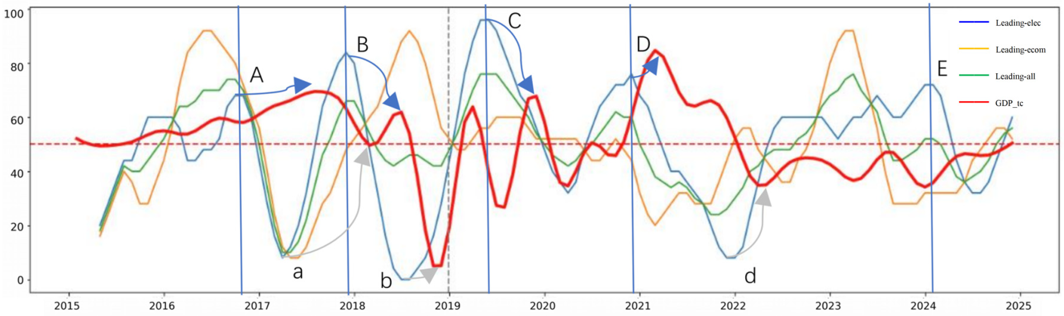
For the results of the business cycle index, the results of the leading index perform well and have strong interpretability. For example, in Figure 4, the leading CI has a local high in October 2020, and the TC series of GDP reaches a local high in March 2021, with the high of the leading CI advancing 5 months relative to GDP (marked by the red vertical line in the chart), and the leading CI has a local low in November 2021, and the TC series of GDP reaches a local low in April 2022, with the low of the leading CI also advancing 5 months relative to GDP. Relative to GDP, this is also five months earlier (marked by the green vertical line in the figure). All three leading indices show an upward trend in the second half of 2024, and based on the five-month lead of the leading indices, it can be predicted that Guangxi’s economy will maintain an upward trend in the first half of this year. Overall, the effectiveness of CI and MDI based on electricity indicators is better than that based on economic indicators. This is basically consistent with the research findings of Li et al. (2023) [13]. One possible explanation for this is that electricity indicator data relies on physical statistics from electricity meters and is more accurate than economic indicators that have been calculated and statistically analyzed.

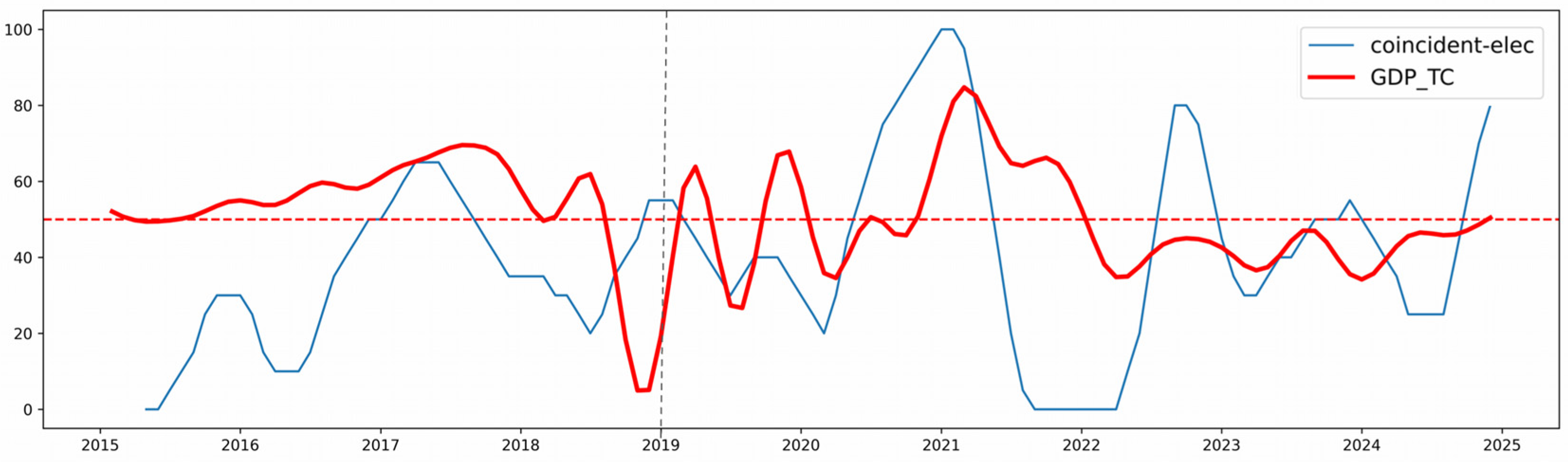
For the results of the coincident index, we use the TC series of GDP as a reference, and the coincident index has relatively good interpretability. For example, in Figure 5, in February 2020 (marked by the blue vertical line in the figure), the CI series is found to have a common low with the GDP series (the lows are two months apart, which is approximated as an overlap), in March 2021 (marked by the red vertical line in the figure), the CI series is found to have a common high with the GDP series (the highs are one month apart, which is approximated as an overlap), in April 2022 (marked by the green vertical line in the figure) The CI series and the GDP series are found to share a common low point. in the second half of 2024, the coincident CI shows a stabilizing trend, suggesting that the Guangxi economy has bottomed out and stabilized in the second half of last year.

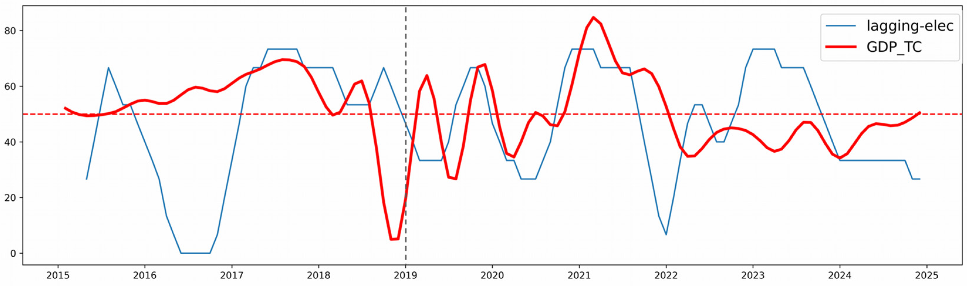
Relatively speaking, the results of the lagging index perform poorly and have weak interpretability. There may be two main reasons for this. Firstly, the number of indicators that make up the lagging index is relatively small. Secondly, the lagging statistical characteristics of the lagging indicators are not very significant (as shown in Table 1).

Comparing the overall results of CI and MDI, the CI index performs better than MDI. This conclusion is consistent with the findings of Dong et al. (1998) [20], OECD (1987) [32], and the Investigation Department of Japan Economic Planning Agency. A common explanation for this conclusion is that the calculation of CI is not limited by the number of indicators, while the calculation of MDI is not only affected by the number of indicators but also by the choice of moving average method, which is consistent with the comparative conclusion of CI and MDI in Section 3.

6. Conclusions

By constructing and analyzing the business cycle analysis system of Guangxi Province from the perspectives of electricity data, economic indicators, and a combination of both, we can draw the following conclusions. First, based entirely on electricity consumption indicators, the regional business cycle analysis system can be reconstructed, thereby improving the timeliness of the calculation results of the business cycle analysis system and enriching the screening range of business cycle indicators. This conclusion indicates that our proposed assumption 3 is correct. Second, the effectiveness of CI and MDI based on electricity indicators is better than that based on economic indicators. This indirectly indicates that the our proposed assumption 1 is correct. Third, in terms of benchmark indicator selection, using monthly GDP as the benchmark indicator is better than using monthly retail sales as the benchmark indicator. This conclusion indicates that the our proposed assumption 2 is correct.

In the future, we plan to work on the following aspects to further improve the applicability of the regional economic business cycle analysis system constructed on the basis of the power indicator data: first, in terms of forecasting, we will introduce the BB turning point method, combine the currently compiled CIs and MDIs, and compile a timed table for economic cycle forecasting to improve the forecasting ability of the system. Second, in the indicator screening method, a machine learning algorithm is introduced while combining the existing K-L information quantity method and time difference correlation coefficient method to further improve the effectiveness of indicator screening. Third, in the benchmark cycle determination, in addition to considering the monthly GDP, the table of major events of Guangxi’s economic development is also introduced to compile the benchmark cycle table of Guangxi’s economic cycle. Fourth, in the indicator weight determination method, an intelligent search algorithm is introduced to realize the intelligent selection of weights for CI calculation and MDI calculation. Fifth, in the scope of indicators, in addition to increasing the data of power indicators such as the volume of OEE, the same high-frequency and timely Baidu search index data can be introduced to expand the scope of indicator selection.