An Improved Tiered Electricity Pricing Scheme Considering Energy Saving and Carbon Reduction, Cross-Subsidy Handling, and User Demands

Abstract

The electric power industry is not only facing the pressure from the reduction of industrial and commercial electricity prices to stimulate the significant growth of demand, but also facing the increasingly serious pressure of unreasonable consumption caused by cross-subsidies; the cross-subsidy mitigation effect and energy-saving effect of the current tiered electricity price policy have basically disappeared. This article examines the main variables that affect the electricity demand and carbon emissions in order to develop a better tiered electricity pricing scheme that can effectively manage cross-subsidies in electricity prices while simultaneously saving energy and lowering carbon emissions. The China Statistical Yearbook’s electricity balance sheets for 2013–2020 are used in this article, along with pertinent data from the State Grid Corporation of China and the China Statistical Yearbook for 2006–2016. It builds an electricity demand model for classified users by using the time series analysis method and multiple statistical regression method. The variables are then subjected to a Granger causality test and a cointegration test in this article. The analysis shows that the adjustment of the electricity price policy has a significant impact on energy-saving and carbon reduction, and for residential electricity consumption, the income variable is the main factor affecting the electricity demand. We take residents’ affordability as the constraint condition for dividing the range of electricity and determining the beneficiary group, take the carbon emission responsibility target and the cross-subsidy degree alleviation target as constraints in determining the tiered price difference, propose an improvement scheme for the tiered electricity price, and carry out the sensitivity analysis of the influence between the parameters. The results show that the optimization improves the precision of the cross-subsidy treatment and significantly improves the effects of energy conservation and emission reduction.

1. Introduction

A key component of attaining high-quality development, according to the report of the 20th National Congress of the Communist Party of China, is encouraging the economy and society to grow in a green and low-carbon manner [1]. In addition, the report also highlights the necessity of promoting carbon peaking and carbon neutrality in an active and responsible manner, as well as accelerating the green transformation of the development mode. Additionally, it promotes the economic and efficient use of all resources, the implementation of a comprehensive strategy for resource conservation, the advancement of the energy revolution, the gradual transition to a system of “Dual control” over the overall quantity and intensity of carbon emissions, the promotion of green consumption, and the development of low-carbon and green production and lifestyle patterns [2]. China’s yearly carbon emissions are predicted to reach over 10 billion tons in 2030, which corresponds to a peak of almost 12 billion tons. With over 40% of the total, the power industry is crucial to reaching the “Double Carbon” target [3]. Currently, there are two main obstacles to green development in the area of electricity consumption: First, the structure and level of electricity prices are severely distorted by China’s long-standing and intricate electricity price cross-subsidy, which leads to excessive electricity use and high power intensity [4,5,6]. Second, because the two price reduction initiatives for general industry and commerce have led to a significant increase in the demand for power, there is now additional pressure on energy conservation and emission reduction. Furthermore, by denying some target groups the subsidies to which they are legally entitled, the one-way price reduction has rendered the subsidy system ineffectual [3,5]. On the other hand, the tiered electricity price policy must fairly and accurately reflect the disparities in the electricity consumption demands and power consumption patterns among different groups. However, there is still a gap between the current policy and this goal, which requires further improvement. At present, the reform of the electricity market is being actively promoted, with the goal of creating a fairer, more efficient, and more competitive environment. Optimizing the electricity price mechanism is a critical link. As a result, while the tiered electricity price policy includes a price penalty mechanism for high-consumption groups, it fails to provide adequate incentives for lower-tier users. Therefore, it is of great significance to study the electricity demand situations and influencing factors of different users, explore how to address the issue of inaccurate electricity price cross-subsidies, figure out how to enhance the subsidy efficiency in combination with the goals of energy conservation and carbon reduction, and propose an improved tiered electricity price scheme that can more reasonably and accurately reflect the differences in electricity consumption demands and power consumption patterns among different groups. This is crucial for reasonably guiding users’ electricity consumption behaviors, promoting the energy consumption revolution, and facilitating energy conservation, carbon reduction, and efficiency improvement.

The remainder of our study is organized as follows: In Section 3 of this article, the electricity balance sheets from the China Statistical Yearbook for the period 2013–2020, as well as the relevant data from the China Statistical Yearbook and the State Grid Corporation of China from 2006–2016, are utilized to analyze the changing trends of the proportion of residential electricity consumption and electricity bill expenditure in disposable income, as well as the electricity consumption of classified users and the influence. In Section 4 of this article, the multiple statistical regression and time series analysis methods are used to create an electricity demand model for classified users. Following that, cointegration and Granger causality tests are performed on the variables, and the effect of price variables on electricity consumption is examined. In Section 5, we summarize the regression results of the electricity demand function models for various user types. This subsection examines the impact of a policy to reduce electricity prices for industrial and commercial use on carbon emissions, as well as the degree to which each independent variable influences the per capita electricity consumption. In Section 6, we examine the improved tiered electricity price scheme and its impact on emissions reduction. This section proposes an improved tiered electricity price scheme based on the targets of resident affordability, carbon emission responsibility, and reducing the level of cross-subsidies. We performed a sensitivity analysis of the impacts between the parameters. Meanwhile, an effect analysis of the impacts brought about by the improved scheme is also conducted. The final section consists of the conclusions, suggestions, and outlooks.

2. Literature Review

Implementing a tiered electricity pricing policy to address cross-subsidies and so encourage energy conservation, carbon reduction, and efficiency is currently a well-established approach. Relevant research and opinions can be summed up in the following two ways.

First, the effects of cross-subsidy electricity prices on efficiency, carbon reduction, and energy conservation were examined. Using the Ramsey pricing formula, Tang and Yang [5] calculated that the structural distortion of China’s power prices between 2007 and 2011 was between 25% and 46%, and that the cross-subsidy raised annual emissions by 130,000 tons of sulfur dioxide and 20 million tons of carbon dioxide. According to a 2007 analysis of China’s electricity usage data by Lin et al. [7], the removal of the cross-subsidy for household electricity consumption would result in a 35.71 billion kWh reduction in electricity consumption and a 23.27 million ton reduction in CO₂ emissions. Xie and Zhang [8] empirically examined the effects of electricity price cross-subsidies on the efficiency of China’s industrial green development through the factor inputs and cost mechanisms, using a sample of 30 Chinese provinces and cities from 2007 to 2013. The eastern region was more adversely affected than the central and western regions. Burke and Kurniawati [9] verified that Indonesia’s electricity price reductions are cross-subsidized, saving 7% of the annual electricity usage and lowering carbon emissions through increased electricity consumption efficiency. Carlos [10], Bhattacharyya [11], Gelan [12], and Andor and Voss [13] found that price subsidies for electricity are mostly effective in fostering technological advancement and the growth of renewable energy, and direct subsidies for power generation and storage. It can effectively lower the energy intensity and encourage the use of a green supply. Developing nations mostly target low-income populations and particular industries, and inclusive subsidy policies lessen the incentive for innovation, impede marketization, and impede the transition to green development.

Second, there is a wealth of research on the mitigating impacts of cross-subsidies and the energy-saving and carbon-reducing implications of the tiered electricity pricing structure. According to Xue and Chen et al. [14], Ma and Zhang [15], and Liu and Zhu [16], the implementation of a tiered electricity pricing policy could reduce environmental pressure by lowering carbon emissions, the electricity demand, and the cross-subsidy. However, Qiao [17], Wang and Zhang [18], Sun [19], and Ye et al. [20] found that the design of China’s current tiered electricity pricing scheme is imprecise, the first tier of electricity consumption is too high, the price difference between tiers is too small, and the energy-saving incentive effect of the tiered electricity pricing policy is not particularly effective, with the average household electricity decreasing by only 1%. The degree of cross-subsidy reduction is also not significant enough, and the mitigation degree is between 2.63% and 8.27%. Based on Tian and Feng [21] and Liu [22], the current tiered electricity pricing policy’s energy-saving and environmental effects have vanished because the policy’s timeliness has weakened, its expected effect has vanished, and the steepness of the incremental tiered electricity pricing structure in developed regions is lower than in less developed regions.

Furthermore, in their research on tiered electricity price models and energy policies, Liu Zimin et al. [16] viewed residents’ consumption of energy sources such as electricity and gasoline as individual carbon trading behaviors. They created the electricity consumption tiers of the tiered electricity price by calculating the equilibrium carbon price of individual carbon trading behaviors. Wang Ting et al. [23] developed a carbon emission quota bidding game model with the goal of maximizing utility in order to compare the differences in the average annual electricity demand between the individual carbon trading mechanism and the tiered electricity pricing mechanism. Shaban et al. [24] developed a Mixed-Integer Quadratic Programming (MIQP) load scheduling model to investigate ways to reduce household energy costs. This model took into account Egypt’s Inclining Block Rate (IBR) of electricity prices, as well as the net metering system, which includes a domestic Photovoltaic (PV) system.

Gunkel et al. [25] investigated the effects of three different pricing methods on consumers’ electricity costs, taking into account various preferences, local network characteristics, and cost allocation factors. Igancio et al. [26] established a residential electricity demand structure model for the ladder electricity price structure in Mexico based on the utility maximization and water demand model. Kim [27] used the marginal electricity price response of consumers to conduct ladder electricity pricing.

In conclusion, the majority of the literature currently in publication examines the effects of cross-subsidies and tiered electricity pricing on green development. It also addresses issues like the need to address cross-subsidies, enhance the tiered electricity pricing policy, and increase electricity prices to encourage carbon reduction and energy conservation, among other things. However, there has been little research on “how to solve the problem” by combining energy-saving and cross-subsidy objectives to design or improve a tiered electricity pricing system. The relevant literature on tiered electricity prices and energy conservation focuses primarily on investigating the relationship between individuals, electricity consumption, and the design of tiered electricity pricing from an energy perspective. What sets this article apart is that our modeling attempts to investigate the relationship between the electricity demands of three distinct types of users—residential, commercial, and general industrial—and other variables. In addition, there are relatively few studies on how to solve the problems of inaccurate subsidy recipients and the insufficient coverage of subsidies. Therefore, we establish a classified user electricity demand model, conduct an empirical study using electricity consumption panel data, and uncover the key factors influencing the electricity demand and carbon emissions. Then, we design an improved tiered electricity pricing scheme that can achieve the coordination of multiple objectives, including enhancing the energy-saving and carbon reduction effects, strengthening the alleviating effect of the cross-subsidy, and adapting to the different affordability of residents. Through the effect analysis, the improved scheme can, to a large extent, achieve the goals of more precise subsidy targets, more refined subsidy levels, and the promotion of energy conservation, carbon reduction, and efficiency improvement.

3. Materials and Methods

3.1. Materials

3.1.1. The Changing Trends of the Proportion of Residential Electricity Consumption and Electricity Bill Expenditure in Disposable Income

The overall amount of electricity consumed is increasing quickly due to the economy’s quick development and the notable rise in resident income. To study the changing trends of the proportion of residential electricity consumption and electricity bill expenditure in disposable income, we obtained data from the official website of the electricity balance sheet in the China Statistical Yearbook. After sorting out the data, they are presented in

Table 1. Changes in household electricity consumption and disposable income from 2013 to 2020 in China.

Year	Population Size (Billions)	Residential Electricity Consumption (kWh)		National Disposable Income per Capita			The per Capita Disposable Income of National Residents Divided into Five Equal Groups by Income
							Low-Income Households (20%)	Lower-Middle Households (20%)	Middle-Income Households (20%)	Upper-Middle Households (20%)	High-Income Households (20%)
		Per Capita Electricity Consumption (kWh)	Year-on-Year Growth Rate (%)	Disposable Income (CNY)	Year-on-Year Growth Rate (%)	Ratio of Electricity Bills to Income (%)	Disposable Income (CNY)	Disposable Income (CNY)	Disposable Income (CNY)	Disposable Income (CNY)	Disposable Income (CNY)
2013	13.61	513.52		18,310.8		1.57	4402.4	9653.7	15,698	24,361.2	47,456.6
2014	13.68	524.56	2.15	20,167.1	10.14	1.46	4747.3	10,887.4	17,631	26,937.4	50,968
2015	13.75	550.18	4.88	21,966.2	8.92	1.4	5221.2	11,894	19,320.1	29,437.6	54,543.5
2016	13.83	608.89	10.67	23,821	8.44	1.43	5528.7	12,898.9	20,924.4	31,990.4	59,259.5
2017	13.9	625.54	2.73	25,973.8	9.04	1.35	5958.4	13,842.8	22,495.3	34,546.8	64,934
2018	14.05	715.87	14.44	28,228	8.68	1.38	6440.5	14,360.5	23,188.9	36,471.4	70,639.5
2019	14.1	754.4	5.38	30,732.8	8.87	1.33	7380.4	15,777	25,034.7	39,230.5	76,400.7
2020	14.12	775.42	2.79	32,188.8	4.734	1.31	7868.8	16,442.7	26,248.9	41,171.7	80,293.8
Average value	13.88	633.85	6.15	25,173.6	8.4	1.4	5943.5	11,769.6	21,317.7	33,018.4	63,062

Note: compiled from the China Statistical Yearbook.

. Based on the data from the China Statistical Yearbook, a substantial increase in electricity consumption in 2019 is evident. Compared to 2006, the total electricity consumption, industrial electricity consumption, and domestic electricity consumption in 2019 increased by 2.62 times, 2.39 times, and 3.27 times, respectively (the data can be found on the official website of China: https://www.stats.gov.cn/sj/ndsj/ (accessed on 12 March 2024)). The percentage of industrial electricity consumption fell from 74.3% to 67.7%, while residential electricity consumption rose from 11.4% to 14.2%, with residential electricity consumption growing at a faster rate than industrial electricity consumption, according to the structural change trend analysis. The degree of the subsidy and the amount of subsidized electricity consumed are positively correlated with the cross-subsidy scale. The scale of the subsidy increases with the amount of subsidized electricity [22]. The cross-subsidy of electricity prices in China currently accounts for about 50%, amounting to 250 billion CNY [19,28]. Since the removal of the cross-subsidy will impact residents’ affordability, and based on the fundamental policy of the universal service of electricity, the Chinese government has not changed the price of electricity for over ten years. Furthermore, as residents continue to receive industrial and commercial subsidies, the scope of cross-subsidies will grow, increasing the burden on industrial and commercial users [21,29].

The affordability of removing or reducing cross-subsidies in electricity prices is indicated by the ratio of residents’ electricity expenses to their disposable income. The average annual growth rate of the residents’ disposable income is 8.40%, which is much higher than the growth rate of the residents’ electricity consumption. Table 1 shows that the per capita consumption of electricity during the eight years from 2013 to 2020 was 633.85 kWh, with an average annual growth rate of 6.15%. With an annual average of 1.40%, the per capita electricity expenditure per resident as a percentage of disposable income declines annually. Residents’ disposable incomes vary greatly; the incomes of upper-middle-class and high-income groups are 10.61 and 5.56 times higher, respectively, than those of low-income groups. This suggests that middle-class and upper-class groups are more tolerant of changes in price policy.

3.1.2. Electricity Consumption of Different Types of Users and Influencing Factors

The total electricity consumption in residential settings is determined by two factors: the population size and per capita electricity consumption. The per capita electricity consumption of residents is affected by electricity costs and income levels [5]. Rising income levels lead to an increased electricity demand and higher carbon emissions [30]. On the contrary, when electricity prices go up, electricity consumption decreases, and carbon emissions are curbed [5]. Lowering industrial and commercial electricity prices reduces businesses’ electricity costs, increases the electricity demand, and raises carbon emissions [27]. Apart from electricity prices, factors like the economic growth rate, industrial structure, and the output value of industrial and commercial sectors also influence carbon emissions from industrial and commercial power use [7]. In the European region, some of the literature holds the view that factors such as income, sunshine duration, and temperature fluctuations can also have a positive impact on the electricity consumption [31]. Moreover, the elasticity of the electricity demand is influenced by income, regional differences, and the electricity price structure [32]. We posit that for residential electricity consumption, higher incomes lead to greater electricity usage, higher electricity prices curb excessive consumption, and larger household sizes result in a higher demand. For commercial and general industrial sectors, higher electricity prices reduce consumption, while increased output boosts electricity usage. Based on these insights, we propose the following hypotheses:

H1a:

Residential electricity consumption is inversely proportional to residential electricity prices.

H1b:

Residential electricity consumption is directly proportional to residential income.

H1c:

Residential electricity consumption is directly proportional to the average household population size.

H2a:

Commercial electricity consumption is inversely proportional to commercial electricity prices.

H2b:

Commercial electricity consumption is directly proportional to commercial output value.

H3a:

General industrial electricity consumption is inversely proportional to general industrial electricity prices.

H3b:

General industrial electricity consumption is directly proportional to the general industrial output value.

In this paper, data such as the population size, average household size, per capita electricity consumption, average electricity price at the consumer end, per capita disposable income, commercial electricity price, output value of the tertiary industry, electricity consumption of non-general industries (nationwide), and the proportion of electricity consumption of non-general industries of the State Grid Corporation of China in the total industrial electricity consumption are downloaded from the official websites of the China Statistical Yearbook and the State Grid Corporation of China (the data can be found on the official website of China: https://www.sgcc.com.cn/html/sgcc_main/gb/index.shtml (accessed on 12 March 2024)). The data on the electricity consumption of various types of users and their influencing factors from 2006 to 2016 are sorted out, as shown in

Table 2. Electricity consumption and influencing factors of various users from 2006 to 2016 in China.

Year	Electricity for Urban and Rural Residents					Commercial Electricity			General Industrial Electricity
	Population Size (Billions)	Average Household Size (Persons/Household)	Per Capita Electricity Consumption (kWh)	Average Electricity Price to Household (CNY/kWh)	Disposable Income per Capita (CNY)	Consumption of Commercial Electricity Price (Billion kWh) ①	Commercial Electricity Price (CNY/kWh)	Commercial Output Value (Billion CNY) ②	Non-General–General Industrial Electricity Consumption (National) ③	Non-General Industrial Prices (CNY/kWh)	Proportional Conversion of Industrial Output Value (Billion CNY) ④
2006	1.314	3.17	247.49	0.5024	7228.8	147.98	0.8742	9175.97	2870.5	0.6952	1246.091
2007	1.321	3.17	274.26	0.5143	8583.5	183.4	0.8797	11,581.07	3298.7	0.7085	1495.845
2008	1.328	3.16	331.02	0.5111	9956.5	201.65	0.8741	13,680.58	3173.1	0.7386	1646.339
2009	1.335	3.15	364.94	0.512	10,977.5	229.43	0.8692	15,474.79	3430.4	0.7748	1763.998
2010	1.341	3.10	382.18	0.5135	12,519.5	315.48	0.8719	18,203.80	3516.4	0.8187	1880.833
2011	1.347	3.02	417.22	0.5169	14,550.7	500.52	0.8424	21,609.86	4134.1	0.8205	2325.436
2012	1.354	2.98	459.31	0.5261	16,509.5	526.92	0.8774	24,482.19	4719.2	0.8684	2720.969
2013	1.361	2.97	513.52	0.5461	18,310.8	413.09	0.9238	27,795.93	5406.5	0.8747	3063.590
2014	1.368	2.97	524.56	0.5422	20,167.1	479.27	0.9087	30,805.86	5076.3	0.878	2909.392
2015	1.375	3.10	550.18	0.5417	21,966.2	521.72	0.8873	34,614.97	5318.1	0.8629	3027.124
2016	1.383	3.11	608.89	0.5419	23,821.0	583.87	0.8402	38,336.50	5697.8	0.8195	3277.749
Average value		3.08	424.87	0.5244	14,962.8	373.01	0.8772	22,341.96	4240.1	0.8054	2305.215

Note: The above data are based on the 2006–2016 China Statistical Yearbook and relevant data from the State Grid, among them: ^① Refers to the electricity consumption of commercial electricity price, which is converted according to the ratio of commercial electricity from the State Grid. ^② Commercial output is replaced by tertiary industry output; ^③ Refers to the electricity consumption of non-general industrial (general industrial) electricity prices, which is converted according to the proportion of non-general industrial electricity in industrial electricity of the national grid. ^④ According to the proportion of non-general industrial electricity in industrial electricity of the State grid.

below. Among them, the “Consumption of commercial electricity price” is calculated by multiplying the proportion of the commercial electricity quantity of the State Grid Corporation of China by the total electricity quantity. The “Commercial output value” is replaced by the data of the output value of the tertiary industry. The “Non general-general industrial electricity consumption” is obtained by multiplying the proportion of the electricity consumption of non-general industries of the State Grid Corporation of China in the total industrial electricity consumption by the total industrial electricity consumption. The “Proportional conversion of industrial output value” is calculated by multiplying the proportion of the electricity consumption of non-general industries of the State Grid Corporation of China in the total industrial electricity consumption by the total industrial output value.

In order to define the variables systematically, in addition to providing a more detailed textual explanation directly under the model, we have also created a variable definition.

3.2. Methods

In China, cross-subsidies for electricity prices are processed in accordance with the cost-internalization mechanism of power grid enterprises. In this system, commercial and industrial enterprises bear the cross-subsidies, while residential and agricultural electricity consumers enjoy them. Additionally, the price of electricity and the consumption of electricity by various users have an impact on each other, which ultimately affects the overall effect of carbon reduction and energy conservation [22,26]. Therefore, this article builds a model of classified user electricity consumption and examines the factors that influence it.

3.2.1. Electricity Demand Function Model of Classified Users

In order to explore the correlation between the variables in Table 2 and the electricity demands of classified users, we take the electricity consumption as the dependent variable and the influencing factors of electricity consumption as the independent variables. In the first step, we first create scatter plots between the dependent variable and each independent variable. It is found that there is no obvious curvilinear relationship between the average household size and residential electricity consumption, as well as between the commercial electricity price and commercial electricity consumption. However, there is a linear relationship between other variables and the electricity consumption of users. In the second step, we conduct a correlation analysis between the dependent variable and each independent variable, and the results are shown in

Table 3. Correlation analysis.

	Population Size	NHom	QRes	PRes	IRes	QBus	PBus	GDPBus	QInd	PInd	GDPInd
population size	1
NHom	−0.5821	1
QRes	0.9963	−0.603	1
PRes	0.9184	−0.6378	0.9254	1
IRes	0.997	−0.5792	0.9921	0.9301	1
QBus	0.9192	−0.6987	0.9102	0.7827	0.9175	1
PBus	0.0886	−0.4198	0.1103	0.4153	0.1058	−0.0841	1
GDPBus	0.9961	−0.5524	0.9903	0.9241	0.9993	0.9129	0.0824	1
QInd	0.9635	−0.6638	0.9693	0.9682	0.9724	0.8964	0.2252	0.9684	1
PInd	0.8468	−0.8592	0.8534	0.8098	0.8295	0.8518	0.3382	0.8115	0.84	1
GDPInd	0.9739	−0.7012	0.9812	0.9511	0.977	0.9247	0.1966	0.9712	0.9933	0.8809	1

. As can be seen from Table 3, per capita electricity consumption (Q_Res) is highly correlated with the population size, average household size (N_Hom), household electricity price of commercial (P_Bus), and per capita disposable income (I_Res). The per capita electricity consumption of commercial electricity consumption (Q_Bus) is highly correlated with the commercial electricity price (P_Bus) and the output value of the commercial industry (GDP_Bus). The per capita electricity consumption of general industrial electricity consumption (Q_Ind) is highly correlated with the price of non-general industries (P_Ind) and the output value of non-general industries (GDP_Ind).

In the third step, according to the curve fit result, the categorized user electricity demand function model is constructed as follows:

$$\mathrm{l}n{Q}_{Res}={\alpha }_1+{\beta }_{11}\ln P_{Res}+{\beta }_{12}\ln I_{Res}+{\beta }_{13}\ln N_{Hom}+{\epsilon }_1$$

(1)

$$\ln Q_{Bus}={\alpha }_2+{\beta }_{21}\ln P_{Bus}+{\beta }_{22}\ln GD{P}_{Bus}+{\epsilon }_2$$

(2)

$$\ln Q_{Ind}={\alpha }_3+{\beta }_{31}\ln P_{Ind}+{\beta }_{32}\ln GD{P}_{Ind}+{\epsilon }_3$$

(3)

In Formulas (1)–(3), $Q_{Res}$, $Q_{Bus}$, and $Q_{Ind}$ denote the per capita electricity consumption of residents, commercial electricity consumption, and general industrial electricity consumption; $P_{Res}$, $P_{Bus}$, and $P_{Ind}$ are the household electricity prices of residential, commercial, and non-general–general industrial users, respectively; $I_{Res}$ is the disposable income of the residents; $N_{Hom}$ is the average population size of the household; $GD{P}_{Bus}$ and $GD{P}_{Ind}$ are the commercial output value and the general (non-general) industrial output value, respectively; ${\alpha }_i$ is a constant; ${\beta }_{i1}$ is the elasticity coefficient; and ${\epsilon }_i$ is the random error term, in which $i=1,2,3$ denotes the three categories of residential, commercial, and general industry users. In order to avoid the issue of “pseudo-regression” and ascertain whether there is a causal and long-term stable relationship between the aforementioned variables and the corresponding dependent variables, the Cointegration and Granger causality tests must be performed.

3.2.2. The Improved Tiered Electricity Pricing Scheme Based on Precise Handling of Cross-Subsidies

This paper considers the careful management of cross-subsidies and green development as joint goals for the creation of a tiered electricity pricing structure, which contains three objectives: First, screening the target group and determining the accuracy of the subsidy targets based on the affordability of residents and the fairness of subsidies principle. Second, in accordance with the demands of green development and emission reduction targets, the degree of cross-subsidies for residents of various income levels or the extent of their reduction should be determined using the cost pricing principle in order to achieve a fine match between cross-subsidy handling policies and subsidy targets. Third, the effects of emission reduction should be measured in order to achieve the precise effects of promoting green consumption.

The analysis of the residential electricity demand function model shows that the primary driver of the demand growth is the rise in resident income. Table 2 shows that in 2016, residents’ disposable income was 3.3 times higher than that of 2006, and per capita electricity consumption was 2.5 times higher than that of 2006. Moreover, residents’ affordability for the elimination or reduction of the cross-subsidy of electricity prices has increased significantly. There is a significant disparity in residents’ disposable income (Table 1). High-income, upper-middle-income, middle-income, and lower-middle-income households are 10.72, 5.70, 3.72, and 2.29 times higher than low-income households, respectively.

This paper proposes the following design concept for the tiered electricity pricing improvement program (Figure 1):

Using residents’ income as the primary parameter, Model (4) estimates the electricity consumption of various income levels based on the panel data of national or various provincial and municipal incomes ($I_j$) and the coefficient of residents’ income–demand elasticity (${\beta }_{12}$). The objects of the cross-subsidy and the extent of the subsidy are then established in accordance with this estimated electricity consumption, which serves as the boundary electricity volume for each tier of the tiered electricity pricing system.

$$Q_j={\beta }_{12}{I}_j$$

(4)

The price difference is ascertained in the second step. There are two methods that can be used. The price–demand elasticity coefficient (${\beta }_{11}$) is used to predict the electricity savings after the tiered price difference is established based on the goal of reducing cross-subsidies. Second, the price differences that must be adjusted for each tier (typically the second and third tiers) are computed using the price–demand elasticity coefficient, and the target electricity savings for energy conservation are established in accordance with the emission reduction target.

The third step is to measure the total amount of emissions that can be reduced. Based on the electricity savings calculated by the first method, combined with the target electricity savings amount in the second method and the grid baseline emission factor, one can calculate the total amount of emissions that can be reduced. The formula is as follows:

$$\Delta C_E=e{\displaystyle \sum T_{Res}}\times P_{R_o}-j\times (Q_j-Q_j-1)\times \Delta P_j/P_0\times {\beta }_{11}\times O_M$$

(5)

where $\Delta C_E$ is the amount of carbon emissions that can be reduced; $T_{Re\mathrm{s}}$ is the total population of residents; $P_{R_o-j}$ represents the ratio of the number of residents subject to the j-th tier of the electricity price to the total number of residents; $Q_j$ is the upper boundary electricity consumption of tiered j; $Q_{j-1}$ is the upper boundary electricity consumption of tiered j−1; $\Delta P_j$ represents the variation value of the electricity price at the j-th tier; $P_0$ is the baseline electricity price of residents; ${\beta }_{11}$ is the price–demand elasticity coefficient of residents; and $O_M$ is the baseline emission factor of the power grid. Then, we can calculate the overall amount of emission reduction based on the baseline emission factor of the power grid, the projected energy-saving electricity consumption of the first method, or the energy-saving target electricity consumption of the second method.

The fourth step is the dynamic adjustment process. We can dynamically modify the price differentials and tiered electricity consumption at the end of the subsequent year or specific cycle in response to changes in relevant variables like the price elasticity, income growth, and emission reduction targets.

We used 2016 data as a base. Then we calculated the monthly average household (3.11 persons/household) and annual per capita electricity consumption for various income levels, from low to high. From low to high income levels, the data are as follows: 208 kWh/year∙person (54 kWh/month∙households), 385 kWh/year∙person (100 kWh/month∙households), 547 kWh/year∙person (142 kWh/month∙households), 744 kWh/year∙person (193 kWh/month∙households), and 1165 kWh/year∙person (302 kWh/month∙households), respectively. Of these, 20% of high-income groups consumed around 38.2% of the electricity, while 40% of upper-middle-income and high-income groups consumed 62.6%. The electricity consumption of high-income, upper-middle-income, middle-income, and lower-middle-income homes is 5.6, 3.6, 2.6, and 1.9 times higher than that of low-income households, respectively.

China has been implementing a tiered electricity pricing policy (No. 2617, [2011] of the National Development and Reform Commission) since 2004. Residential electricity is priced in three tiers, with the first tier covering 80% of residential users in each province and city and not adjusting prices. The price of each kWh should be raised by at least 5 cents in the second tier, which should cover 80% to 95% of residential users; the third tier, which covers 95% to 100% of residential users, should raise prices by roughly 0.3 CNY per kWh. Relevant scholars have determined that the current average of the first, second, and third tiers are 0–120 kWh/month·households, 120–400 kWh/month·households, and 400 kWh/month·households and above, based on the weighted average of 31 Chinese provinces and municipalities [19]. Even 20% of high-income households (302 kWh/month) are not included in the tiered electricity price increase, according to a comparison between the model data and the current policy. Rather than designing the tiered electricity pricing policy based on the actual situation of the electricity consumption of various income levels, using the benefit coverage as the primary criterion will also result in a significant “leakage effect” of the cross-subsidy and decrease the effectiveness of income redistribution [5,19]. In actuality, the “rich ride on the poor” phenomenon in the current tiered electricity pricing policy is quite serious [21], departing from the cross-subsidy tiered electricity pricing policy’s goal of the fairness and rationality of the universal service [19,21,22].

In order to better achieve the equity and efficiency goals of the universal service policy, this paper considers the affordability of residents as the constraints of the tiered boundary electricity consumption and beneficiary groups, and implements a precise subsidy policy, with low-income, low-middle-income, and middle-income households as the target of the subsidy (with the number of users accounting for 60%, and the electricity consumption accounting for 37.4%), and with high-income and upper-middle-income households as the target of the cross-subsidy cancellation or reduction (with the number of users accounting for 40%, and electricity consumption accounting for 62.6%). Based on the electricity consumption of users at each income level, the first tier is set at 0–142 kWh/month·households and below; the second tier is set at 142–193 kWh/month ∙ households; and the third tier is set at 193 kWh/month∙households and above. This plan is more comprehensive than the current ladder electricity price classification, increases the electricity consumption limit of the first tier, raises the benefit coverage rate, and reflects equity; it also reduces the “leakage effect” and narrows the second-grade difference, lowers the third threshold tax, and increases the effectiveness of income redistribution [19,21]. In the event that further refinement is required, the electricity consumption of the tiered electricity pricing program is separated into five grades according to the measured tiered boundary electricity consumption.

3.2.3. The Mitigation Effect of Electricity Prices’ Cross-Subsidies

In order to further analyze the relationship between the reduction amount of carbon emissions and the degree of cross-subsidy cancellation, and to explore how much the degree of cross-subsidy cancellation should be determined under different carbon emission targets. We set the degree of cross-subsidy cancellation E_Sub as the independent variable and the reduction in carbon emissions $\Delta C_E$ as the dependent variable.

According to the internationally accepted cross-subsidy measurement model based on the price difference method, the determination of the cross-subsidy amount and the degree of cross-subsidy should satisfy the following formula:

$$Sub=\left(P_0-P_{\mathrm{i}}\right)\times Q$$

(6)

$$D_{Sub}=\left(P_0-P_{\mathrm{i}}\right)/ P_0$$

(7)

where $Sub$ and $D_{Sub}$ represent the cross-subsidy amount and the degree of cross-subsidy for residential users, respectively. $P_0$ represents the benchmark electricity price for residents. The benchmark electricity price for electricity consumption is the reference electricity price in the electricity market, serving as the basic standard of electricity prices, and it reflects the average production cost of electric energy. $P_i$ is the actual electricity price of residents and $Q$ is the electricity consumption of residents. On this basis, the degree of the cross-subsidy of the tiered electricity pricing can be calculated, which is represented by Equation (7). It can be further introduced that $(1-D_{Sub})$ is the degree of cross-subsidy to be reduced under the policy objective, so the degree of elimination of the cross-subsidy is denoted by $E_{S\mathrm{ub}}$, and from this, we can determine the correlation with the electricity price level $P_{\mathrm{i}}$:

$$E_{Sub}=1-D_{Sub}=1-\left(P_0-P_j\right)/ P_0$$

(8)

In addition, the residential price–demand elasticity ${\beta }_{11}$ can be used to measure the reduction in the total electricity demand $Q\_De{c}_{\mathrm{i}}$, which means that there is a correlation between the total electricity demand reduction $Q\_De{c}_{\mathrm{i}}$ and the degree of the cross-subsidy$E_{Sub}$.

$$Q\_D{\mathrm{ec}}_i={\beta }_{11}\times P_i-Q_0$$

(9)

On this basis, referring to the study of Liu Zimin et al. [33], the following model was established by using $\mathrm{MATLAB}$ 2018 software.

$$\Delta C_E={\alpha }_1{E}_{Sub}+{\alpha }_{2}ln{P}_1+{\alpha }_{3}lnQ\_De{c}_1+{\alpha }_{4}lnP\_In{c}_1+{\alpha }_{5}ln{P}_2+{\alpha }_{6}lnQ\_De{c}_2+{\alpha }_{7}ln P\_In{c}_2+\mu$$

(10)

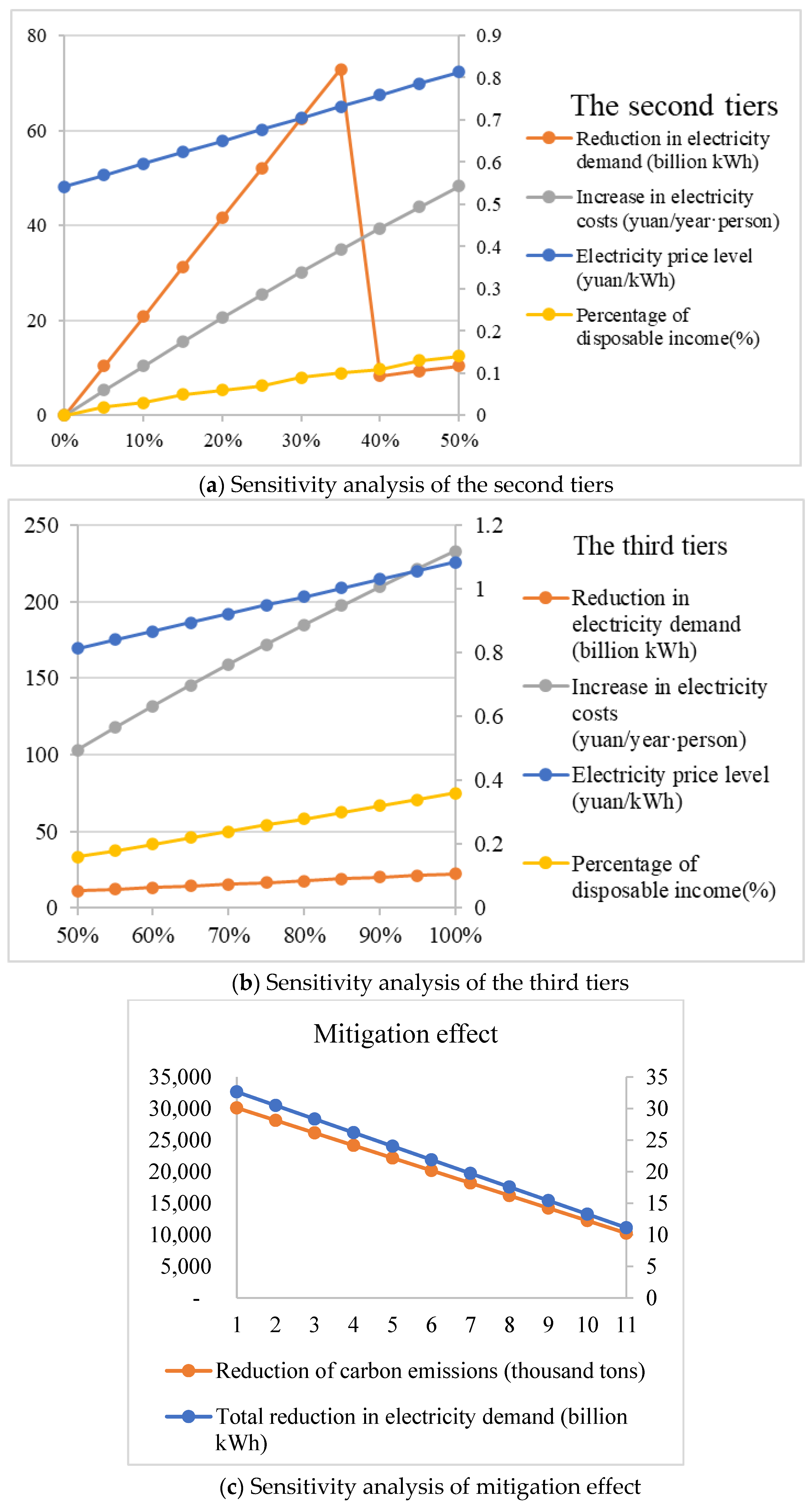
In model (10), $\Delta C_E$ is the reduction in carbon emissions due to the policy impact calculated in model (5); $P_1$ and $P_2$, respectively, represent the electricity price levels under the second-tier and third-tier ladders determined by the policy; $Q\_DE{C}_1$ and $Q\_DE{C}_2$, respectively, represent the total reduced electricity demand under the second-tier and third-tier ladders, both of which are affected by the price–demand elasticity of residents; and $P\_In{c}_1$ and $P\_In{c}_2$, respectively, represent the total increased electricity bills per year under the second-tier and third-tier ladders. Through the sensitivity analysis of the impact of gradually canceling the degree of the electricity price cross-subsidy on residents’ affordability and the emission reduction effect, and in combination with Equation (10), we can determine the degree of the electricity price cross-subsidy that needs to be reduced according to the target emission reduction amount, thus reducing the net loss of social welfare caused by the electricity price cross-subsidy problem.

4. Regression Results of the Electricity Demand Function Models for Various Types of Users

4.1. Test of the Stable Relationship of Variables

To determine whether there is a long-term stable and causal relationship between the above independent variables and the corresponding dependent variables in Models (1)–(3), and to avoid the problem of “spurious regression”, it is necessary to conduct a cointegration test and a Granger causality test. The first step is to determine whether the 10 variables are non-stationary by performing a unit root test on them. The findings indicate that while some variables are first-order integrated variables, others are second-order. The order in which the explanatory variables are integrated must match the cointegration test’s requirements. Therefore, the variables are all differenced at the same order to convert them into stationary sequences, and a cointegration test is carried out on these difference values. The results are shown in

Table 4. Results of the stationarity test for each variable.

Second-Order Differenced Variable	Test Type	ADF Value	1% Critical Value	5% Critical Value	10% Critical Value	Conclusion
Average household size (persons/household)	(c,0,0)	−4.268 **	−4.38	−3.6	−3.24	Stationary
Per capita electricity consumption (kWh)	(c,0,0)	−3.578 **	−3.75	−3	−2.63	Stationary
Average electricity price to household (CNY/kWh)	(c,0,0)	−3.977 ***	−3.75	−3	−2.63	Stationary
Disposable income per capita (CNY)	(c,0,0)	−2.614 *	−3.75	−3	−2.63	Stationary
Consumption of commercial electricity price (billion kWh)	(c,0,0)	−2.752 ***	−3.75	−3	−2.63	Stationary
Commercial electricity price (CNY/kWh)	(c,0,0)	−2.958 **	−3.75	−3	−2.63	Stationary
Business industry (billion CNY)	(c,0,0)	−3.165 **	−3.75	−3	−2.63	Stationary
Non-general–general industrial electricity consumption (national)	(c,0,0)	−5.142 ***	−3.75	−3	−2.63	Stationary
Non-general industrial prices (CNY/kWh)	(c,0,0)	−4.814 ***	−3.75	−3	−2.63	Stationary
Proportional conversion of industrial output value (billion CNY)	(c,0,0)	−2.903 **	−3.75	−3	−2.63	Stationary

Note: The ADF test type is (c, t, k), where c represents the intercept term, t denotes the inclusion of a trend term, and k indicates the lag order; ***, **, and * signify significance at the 1%, 5%, and 10% levels, respectively.

.

According to Table 4’s results, following a second-order difference in the variables, the ADF test statistic for per capita disposable income is higher than the critical value at the 10% significance level; this is also the case for the average household size, per capita electricity consumption, commercial electricity price, commercial industry output value, and industrial output value at the 5% significance level. As a result, the null hypothesis cannot be disproved, proving that all variables are stationary time series with a cointegration relationship and no unit roots.

In order to determine whether there is a statistical relationship in the economic sense among the above variables, Granger causality test models for per capita residential electricity consumption, commercial electricity consumption, and general industrial electricity consumption are established, respectively, according to Models (1)–(3). The test results are shown in

Table 5. Granger causality test between electricity consumption and independent variables of various users.

Test Variable	Original Hypothesis Causation	F Value	p Value	Test Conclusion
PRes	The electricity price of household users is not the Granger cause of per capita electricity consumption of residents	150.010	0.000	The electricity price of household users, disposable income of residents and average household population size are the Granger reasons of the per capita electricity consumption of residents
IRes	Disposable income of residents is not the Granger cause of per capita electricity consumption of residents	198.884	0.000
NHom	Average household size is not a Granger reason for per capita residential electricity consumption of residents	46.773	0.001
PBus	The commercial electricity price of household users is not the Granger cause of commercial electricity consumption	158.494	0.000	The commercial electricity price of household users and commercial output value are Granger reasons of commercial electricity consumption
GDPBus	Commercial output value is not Granger cause of commercial electricity consumption	428.297	0.002
PInd	Non-general–general industrial electricity price of household users is not the Granger cause of general industrial electricity consumption	148.319	0.000	Non-general–general industrial electricity price of household users, general (non-general) industrial output is the Granger reason of general industrial electricity consumption
GDPInd	General industrial output value is not the Granger cause of general industrial electricity consumption	46.695	0.001

.

Table 5 demonstrates that the dependent and independent variables of Models (1)–(3) exhibit Granger causality. Consequently, we perform multiple linear regression on the variables using SPSS21.0. In the regression analysis, the forced entry method is used for price variables. Instead of screening these variables, all of them are included in the model. For the other variables, we adopt the stepwise regression method.

Table 6. Power demand function model statistics of various users.

User Category	Model	Model Checking		$\mathbf{Ratio} ({\mathit{\alpha }}_{\mathit{i}}$)			$\mathbf{Ratio} ({\mathit{\beta }}_{\mathit{i}1}$)			$\mathbf{Ratio} ({\mathit{\beta }}_{\mathit{i}2}$)			$\mathbf{Ratio} ({\mathit{\beta }}_{\mathit{i}3}$)			Collinearity Statistic
		R-Square	Modified Sig.F	Unstd. Coeff.	T Value	Sig.	Unstd. Coeff.	T Value	Sig.	Unstd. Coeff.	T Value	Sig.	Unstd. Coeff.	T Value	Sig.	VIF
Residential electricity consumption	1	0.822	0.000	11.703	13.263	0.000	8.806	6.453	0.000							6.675
	2	0.988	0.000	−1.621	−1.276	0.238	−0.529	−0.557	0.592	0.764	10.683	0.000				6.564
	3	0.988	0.000	−1.626	−1.052	0.328	−0.528	−0.516	0.622	0.764	9.765	0.000	0.004	0.007	0.994	1.769
	4	0.988	0.000	−0.929	−3.623	0.006				0.727	27.113	0.000				1.000
Commercial electricity consumption	1	0.001	0.919	26.460	33.024	0.000	−0.624	−0.104	0.919							1.010
	2	0.919	0.000	−5.174	−1.551	0.160	−2.338	−1.287	0.234	1.025	9.506	0.000				1.010
Industrial electricity consumption	1	0.751	0.001	27.299	241.196	0.000	2.519	5.211	0.001							6.130
	2	0.983	0.000	1.601	0.651	0.533	−0.652	−1.966	0.085	0.880	10.455	0.000				6.130

Note: “Modified Sig.F” means the significance result of the F-test after modification or adjustment. “Sig.” is stand for significance and nit refers to the p-value. “VIF” stands for Variance Inflation Factor.

displays the results of the regression for pertinent statistics.

4.2. Impact of Industrial and Commercial Electricity Price Reduction Policy on Carbon Emissions

Since 1 April 2018, China has successively reduced electricity prices for general industrial and commercial users by 10% for two consecutive years, resulting in a 19% compound price cut after two rounds of adjustments. Significant reductions in industrial and commercial electricity prices have stimulated the electricity demand, increased pressure on energy conservation and emission reduction, and led to a certain degree of the proper handling of cross-subsidies. The price-cut policy has accelerated the process of gradually returning residential electricity prices to cost-based pricing. Next, a quantitative analysis of the price-cut policy’s impact on carbon emissions will be conducted.

Through successive tests of the models for the industrial and commercial electricity demand, we discovered that the R-square, T-value, and significance for commercial electricity consumption in Model 1 (where the price of commercial electricity is the independent variable) indicate that the model and price variable coefficients are not statistically significant. Next, we perform a partial correlation analysis of the variables related to the commercial electricity price and consumption using commercial GDP as a control variable. The partial correlation coefficient is −0.414. The elasticity coefficient of the commercial output value–demand ${\beta }_{22}$ is 1.025, indicating that the commercial GDP has a significant influence on the commercial electricity demand. For Model (2), in which the independent variables are the commercial electricity price and commercial GDP, the corresponding coefficient of the commercial GDP variable is statistically significant, with a significance level of 91.9%, meaning Hypothesis 2a and 2b hold.

For general industrial electricity consumption, Model (1) (the independent variable is the general industrial electricity price) and Model (2) (the independent variables are the general industrial electricity price and general industrial GDP) are both statistically significant. In Model (1), the ${\beta }_{31}$ coefficient is 2.519, which is not consistent with reality. The coefficient of the general industrial price variable in Model (2) is ${\beta }_{31}$, and this value represents the price–demand elasticity coefficient of −0.652, and the coefficient of the general industrial GDP variable is ${\beta }_{32}$, which is the elasticity coefficient of the industrial output value–demand and equals 0.880, meaning Hypothesis 3a and 3b hold. Model (2) shows that the influence of the general industrial GDP variable on electricity consumption is greater than the influence of the price variable on electricity consumption. The partial correlation coefficient between the price of industrial electricity and its consumption is −0.571.

The yearly demand for commercial and general industrial electricity will rise by 45.9 billion kWh and 61.8 billion kWh, respectively, following the two price reductions in 2016. The price reduction policy will result in an increase of 99.34 million tons of carbon dioxide emissions, based on the baseline emission factor ($OM$) (0.9224 tCO₂/MWh) averaged by China’s regional grid in 2017.

4.3. The Degree of Influence of Each Independent Variable on per Capita Electricity Consumption

According to Table 6, the Sig. for Model (1) (independent variable: the residential electricity price), Model (2) (independent variables: the residential electricity price and per capita disposable income), and Model (4) (independent variable: the per capita disposable income, others are control variables) concerning per capita residential electricity consumption is 0.000. The R-square indicates that the resolution of the data is 82.2%, 98.8%, and 98.8%, and that all three models are statistically significant. The price variable is statistically significant, as indicated by the coefficients ${\alpha }_1$ and ${\beta }_{11}$ in Model (1), which correspond to t-values ($\ge 1.96$) with Sig. (<0.05); however, the price–demand elasticity coefficient is 8.806, which is not consistent with reality. The t-value corresponding to the coefficients in Model (2) ($\ge 1.96$) with Sig. (<0.05) shows that the coefficient ${\beta }_{12}$ of the variable of disposable income per capita is statistically significant, but ${\alpha }_1$ and ${\beta }_{11}$ are not. Model (2) also demonstrates that the impact of per capita disposable income on per capita electricity consumption is greater than the effect of the residential electricity price on per capita electricity consumption. Therefore, Hypothesis 1a, 1b, and 1c hold. According to Model (4), the coefficient of residential income–demand elasticity is 0.727, and ${\alpha }_1$ and ${\beta }_{12}$ are statistically significant. Model (3) (the independent variables are the residential electricity price, per capita disposable income, and household size) shows that the household size has basically no bearing on the per capita electricity consumption. Accordingly, the corresponding price variable coefficients in Model (2) are not statistically significant since the corresponding price variable coefficients in Model (1) are inconsistent with reality. Thus, using the household size and per capita disposable income as the control variables, this study performs partial correlation analysis on the residential price and per capita electricity consumption variables, yielding a partial correlation coefficient of −0.191. The partial correlation coefficient allows us to assess how much the independent variable influences the dependent variable. This value is essentially in line with the data collected by domestic researchers, including Tang Yaojia and Yang Jian [5], who calculated the elasticity of the demand for the price of electricity for residential use to be −0.324, and Lin Boqiang and Jiang Zhujun et al. [7] who calculated the elasticity of demand for the price of electricity for urban residents to be −0.2149. However, this value shows some differences from the results calculated abroad. The price elasticity in Europe and Central Asia is −0.61, while that in North America reaches −0.63 [30].

5. Analysis of Improved Tiered Electricity Pricing Scheme and Emission Reduction Effects

5.1. The Emission Reduction Effect of the Improved Scheme

According to Table 2, the average yearly rise in home power prices from 2006 to 2016 was 0.715%, or 1.079 times the 2006 price. With a price–demand elasticity coefficient of −0.191 and household power usage of 842.1 billion kWh in 2016, we can determine that the existing tiered electricity pricing strategy only lowers the annual electricity demand by 1.15 billion kWh. The 2017 average OM of 0.9224tCO₂/MWh was used as the basis for the computation; the price difference between grades is too minor, the home power price has not been changed for 11 years, from 2006 to 2016, and the existing tiered electricity pricing scheme has very little impact on reducing emissions and saving energy [17].

The degree of cross-subsidy of residential electricity prices in China is approximately 50% [5,21]. In accordance with the first method of improving the scheme’s price spread design, we use the cross-subsidy mitigation target as the scheme’s constraints and use Equation (4) to calculate the effect of lowering the degree of cross-subsidies on energy conservation and emission reduction. In addition, we use the residents’ growing electricity charges and their percentage of their disposable income (2017) as the reference index of their affordability based on the various cross-subsidies, as determined by their price–demand elasticity. In this paper, we pre-select the second tier of the electricity cross-subsidy to be reduced by 50% (this indicator can be selected according to the policy objectives, see

Table 7. Sensitivity analysis of the impact of cross-subsidy levels on residents’ affordability and emission reduction effects.

Programmatic Portfolio	The Second Tiers					The Third Tiers					Mitigation Effect
	Degree of Cross-Subsidy Elimination (%)	Electricity Price Level (CNY/kWh)	Reduction in Electricity Demand (Billion kWh)	Increase in Electricity Costs (CNY/Year·Person)	Percentage of Disposable Income (%) ①	Degree of Cross-Subsidy Elimination (%)	Electricity Price Level (CNY/kWh)	Reduction in Electricity Demand (Billion kWh)	Increase in Electricity Costs (CNY/Year·Person)	Percentage of Disposable Income (%) ①	Total Reduction in Electricity Demand (Billion kWh)	Reduction in Carbon Emissions (Thousand Tons)
1	50%	0.8129	10.408	48.28	0.14	100%	1.0838	22.242	232.84	0.36	32.649	30,115.7
2	45%	0.7858	9.3669	43.91	0.13	95%	1.0567	21.13	221.32	0.34	30.496	28,129.9
3	40%	0.7587	8.3261	39.44	0.11	90%	1.0296	20.018	209.47	0.32	28.344	26,144.2
4	35%	0.7316	72.853	34.87	0.1	85%	1.0025	18.905	197.3	0.30	26.191	24,158.4
5	30%	0.7045	62.446	30.19	0.09	80%	0.9754	17.793	184.82	0.28	24.038	22,172.6
6	25%	0.6774	52.038	25.41	0.07	75%	0.9483	16.681	172.01	0.26	21.885	20,186.8
7	20%	0.6503	41.631	20.54	0.06	70%	0.9212	15.569	158.88	0.24	19.732	18,201.0
8	15%	0.6232	31.223	15.55	0.05	65%	0.8941	14.457	145.43	0.22	17.579	16,215.2
9	10%	0.5961	20.815	10.47	0.03	60%	0.8670	13.345	131.67	0.20	15.427	14,229.4
10	5%	0.5690	10.408	5.287	0.02	55%	0.8399	12.233	117.58	0.18	13.274	12,243.7
11	0	0.5419	0	0	0	50%	0.8129	11.121	103.18	0.16	11.121	10,257.9

Note: ^① in this study, the ratio of incremental electricity charge to residents’ disposable income is used as an observational parameter for changes in residents’ affordability.

) as the initial target, take a 5% sensitivity ratio (any sensitivity ratio can be set to scale; the lower the ratio, the more meticulous), and carry out the decrement calculation. Then, we reduce the third tier of the electricity cross-subsidy by 100% (cost-based pricing), carry out a decrement calculation at a 5% ratio, and obtain the impact of the degree of cross-subsidies on the sensitivity data analysis of the residents’ affordability and energy-saving and emission reduction effect. The obtained impact is shown in Table 7 and Figure 2.

As can be seen from the two figures above, (a) and (b) in Figure 2, the electricity price of the second tier is lower than that of the third tier. With the increase in the degree of cross-subsidy cancellation, the electricity price gradually rises. In the second tier, the “Reduction in electricity demand” shows a significant increase when the degree of cross-subsidy cancellation reaches 35%, while in the third tier, it remains in a linear state throughout. The change trends of “Increase in electricity costs” and “Percentage of disposable income” are the same. As the degree of subsidy cancellation decreases, both indicators show a downward trend.

In Table 7, columns 2 and 7 show the cross-subsidy mitigation targets, and columns 3 and 8 show the corresponding second- and third-tiered electricity pricing, which can be combined into a single-tiered electricity pricing scheme in any two groups. According to Equation (4), the energy-saving and emission reduction effect of the pricing scheme can be measured. For example, in the combination of Scheme 1 of Table 7, eliminate the third-tiered electricity cross-subsidies, and the price is doubled (1.0838 CNY/kWh) to achieve cost pricing; eliminate the second-tiered cross-subsidies of 50%, the price is increased by 0.5 times (0.8129 CNY/kWh). This pricing scheme reduces the electricity demand by 32.65 billion kWh and will reduce 30.116 million tons of carbon dioxide emissions, which is 28.4 times the emission reduction effect of the current tiered electricity pricing policy. In the specific design, it is also possible to follow the second method of improving the scheme: taking the energy-saving and emission reduction targets as the constraints of the spread design, selecting the degree of cross-subsidies that need to be reduced in each grade according to the sensitivity analysis table, and combining them into the optimal spread ladder tariff scheme.

Table 7 shows that the adjustment of the tiered electricity pricing policy and the implementation of a precise cross-subsidy mechanism can significantly reduce carbon emissions, but still cannot offset the increase in emissions due to the reduction of general industrial and commercial tariffs, and the situation of emission reduction in the field of electricity consumption is becoming more and more serious.

Taking Combination Scenario 1 as an example, Table 7 shows that according to the improved scenario, based on the disposable income of the residents in 2017, the upper-middle-income group spends more on electricity, with costs of 48.28 CNY/year·person, which accounts for 0.14% of their disposable income, and the high-income group spends more on electricity, with costs of 232.84 CNY/year·person, accounting for 0.36% of their disposable income, which is a relatively low percentage. The average annual growth rates of the disposable income of the upper-middle-income and high-income groups measured in Table 1 are 9.13% and 8.16%, respectively. Therefore, when increasing the price difference and eliminating or reducing the cross-subsidy, the impact is minimal, and the proportion of the increase in the electricity fees for the two tiers of residential users is significantly lower than the average annual growth rate of residents’ disposable income.

5.2. The Alleviating Effect of Electricity Price Cross-Subsidy

In order to study the alleviating effect of the electricity price cross-subsidy, we made use of Models (6)–(10) and obtained the following results by performing function fitting in $\mathrm{MATLAB}$ software. The fitting results are shown in

Table 8. The fitting results of the carbon emissions model.

${\mathit{\alpha }}_1$	${\mathit{\alpha }}_2$	${\mathit{\alpha }}_3$	${\mathit{\alpha }}_4$	${\mathit{\alpha }}_5$	${\mathit{\alpha }}_6$	${\mathit{\alpha }}_7$
−5.04	−25.08	5.16	43.22	−3.81	−0.14	2.95

Note: the results in the table are the result of dividing the value by 1000.

.

The results in Table 5, combined with Equation (10), can be used to determine the extent of the cross-subsidy that needs to be reduced based on the targeted emission reductions, thereby reducing the net loss of social welfare caused by the electricity price cross-subsidy problem. For example, if policymakers decide to set the target for emission reduction in the next year at 30 million tons, and we assume that under the second and third tiers of the electricity price, the electricity price levels are 0.6 CNY per kilowatt/hour and 1.1 CNY per kilowatt/hour, respectively, the reduced electricity demands are 9 billion kilowatt/hours and 20 billion kilowatt/hours, respectively, and the increased total electricity charges per person in that year are 45 CNY and 220 CNY, then according to Model (10) and the fitting results in Table 8, the degree of the electricity price cross-subsidy that should be cancelled can be calculated to be 42.697%.

6. Discussion

This paper proposes an enhanced framework for the tiered electricity price policy, exploring the intricate interplay between energy consumption dynamics and electricity price cross-subsidies. We conduct a comprehensive analysis of the new scheme’s potential to drive emission reductions and mitigate cross-subsidy disparities. Through in-depth research, we identify key determinants of electricity consumption: for residential sectors, household income, population size, average household occupancy, and per-unit electricity costs are pivotal; commercial consumption is mainly influenced by commercial electricity rates and the industry output value; and general industrial consumption is closely associated with industrial electricity tariffs and the production volume.

In comparison with international research, Wesley et al. [34] highlight that in-home displays (IHDs) providing real-time electricity consumption feedback to residents represent an additional influential factor. Wemyss et al. [35] demonstrate that social power interventions yield positive and encouraging short-term outcomes in electricity conservation and self-reported behavioral changes. However, these beneficial effects diminish partially within a year. Burney et al. [36] emphasize that the per capita income is the most significant determinant, followed by the share of industry in GDP, years of education, and urbanization levels.

Furthermore, significant regional disparities exist in residential electricity consumption. When analyzing the energy consumption intensity, it is essential to consider the unique resource endowments and infrastructure histories of different countries and regions [37]. Our study provides further evidence that income is the most influential factor in electricity consumption. Consistent with this finding, Jones et al. [38] have identified 62 potential factors influencing residential electricity use, categorized into 13 socioeconomic, 12 residential-related, and 37 appliance-related variables. Notably, in developed countries and regions, these factors interact to generate distinct consumption patterns, reflecting the complex interplay of economic, social, and technological contexts. In the UK, the building area of residential properties, especially the number of rooms and bedrooms, along with the prevalence of regular home-based work, are key indicators reflecting variations in household electricity and gas consumption [39]. In Israel, larger household sizes correlate with lower per capita electricity consumption, and households with members under 40 years old account for the majority of electricity use [40]. In Sweden, factors such as the number of family members, usage of sauna equipment and computers, and heating intensity positively impact electricity consumption [41]. In Australia, extreme weather conditions and consumer behavior significantly shape the energy demand [42]. In the US and Norway, the growth rate of the total energy demand lags behind that of household income, and the per capita energy demand decreases as the number of family members increases [43,44]. Additionally, in the US, factors including the household building area, family size, disposable income, HoH gender, presence of children, and residents’ window-opening behavior all influence residential electricity consumption [45]. In developing countries, different consumption drivers are at play. In Kuwait, the residential lifestyle, electrical equipment usage duration, and air-conditioning settings are crucial for energy consumption [46]. In Burkina Faso, the household income, residential property type and ownership, and furniture inventory significantly impact urban household electricity use [47]. In Taiwan, China, Hung et al. [48] reveals that the relationship between electricity consumption and household size is non-linear, presenting an inverted U-shape, which is only significant during non-summer months.

Regarding the improvement and optimization of the tiered electricity price policy, Ayertey et al. [49] stress the necessity of tailoring the policy to local contexts; otherwise, its effectiveness will be severely limited. Cardenas et al. [50] propose integrating information on heterogeneous price elasticities into the pricing policy, which can reduce residential electricity consumption inequality while maintaining power suppliers’ revenues. Research in Ethiopia shows that when electricity prices are far below the total average cost and constitute a small proportion of household income, the positive electricity conservation effect of the tiered electricity price policy is minimal [51]. Currently, relying solely on energy conservation campaigns proves insufficient for cultivating residents’ environmental awareness [52]. Instead, strategies such as providing real-time electricity consumption feedback, setting personalized consumption targets, and implementing reward systems have been shown to effectively enhance environmental awareness [53,54]. Li et al. [55] finds that women, the elderly, highly educated individuals, and high-income residents play a more prominent role in promoting energy-saving behaviors compared to men, young people, those with lower education levels, and low-income residents. In developed countries like Australia, the energy intensity decreases with increasing expenditure levels [56]. In contrast, in some developing countries such as Brazil and India, the average household energy intensity grows slowly with rising income, even among the highest-income groups [57].

7. Conclusions

China is facing an increasingly serious problem of electricity price cross-subsidy because the residential electricity prices have not been adjusted for more than a decade. Excessive cross-subsidies have led to the distortion of electricity prices, serious problems of irrational consumption, an increase in environmental governance costs, and great difficulties in promoting the energy consumption revolution. The misaligned cross-subsidy policy has led to the phenomenon of “the rich taking advantage of the poor”, resulting in low efficiency in income redistribution. The people-benefiting policy suffers from a serious “leakage effect”, which undermines its fairness. In addition, the current tiered electricity pricing policy has achieved very little in terms of energy conservation, emission reduction, and the alleviation of cross-subsidies due to their inaccurate design.

Under the dual constraints of economic development and environmental pressure, dealing with cross-subsidies through the tiered electricity pricing policy is no longer a one-way issue. Instead, it requires the coordination of multiple objectives such as fairness, efficiency, and green development for improvement. Through empirical research using the electricity consumption data of residential, industrial, and commercial users from 2006 to 2016, we find that:

• Among the factors affecting the electricity demand of different users, the residential electricity demand is highly correlated with the population size, the average household size, the average electricity price per household, and the per capita disposable income; the commercial electricity demand is highly correlated with the commercial electricity price and the commercial output value; and the electricity demand of non-general industrial users is highly correlated with the non-general industrial price and the non-general industrial output value. Among them, residents’ income is a key variable affecting electricity demand.
• By taking residents’ disposable income, carbon emission responsibility targets, and the degree of cross-subsidy alleviation as constraints and then determining the tiered electricity consumption boundaries and price differentials between tiers of the tiered electricity pricing, we can improve the precision of handling cross-subsidies, significantly enhance the effects of energy conservation and carbon reduction as well as the alleviation of cross-subsidies, and promote green consumption.
• Dividing and identifying the target beneficiary groups based on the residents’ income levels can reduce the degree of subsidy mismatch such as “the rich free-riding on the poor” and improve the fairness of universal services.

When formulating residential electricity prices, power companies can conduct more precise pricing according to the characteristics of the electricity consumption needs of different income groups. For example, for low-income groups, since they are more sensitive to electricity prices, power companies can appropriately reduce the electricity prices or provide a certain amount of electricity subsidies to ensure their basic electricity consumption needs for daily life. For high-income groups, the electricity prices can be increased to a certain extent to reflect their higher electricity consumption demand and consumption ability. For commercial and non-general industrial users, according to their correlations with commercial electricity prices, output values, as well as non-general industrial prices and output values, differentiated electricity prices can be formulated for users of different industries and scales to better match their electricity consumption costs and revenues. Since the electricity demand of commercial and non-general industrial users is highly correlated with electricity prices and output values, regulatory authorities can guide the adjustment of the industrial structure by adjusting electricity price policies. At the same time, considering the carbon emission responsibility targets, regulatory authorities can formulate more stringent carbon emission supervision standards for the power industry. Specifically, these standards can require power enterprises to optimize the power source structure, increase the proportion of clean energy power generation, and reduce the carbon emissions from traditional fossil energy power generation. Meanwhile, users can be guided to save energy and reduce emissions through the price mechanism. Higher electricity prices can be imposed on high-energy-consuming and high-polluting enterprises, and certain price preferences or subsidies can be given for clean energy consumption to promote the development of the whole society towards the direction of being green and low-carbon. After comprehensively considering and setting three parameters, namely the residents’ affordability range (for example, taking the proportion of the increased electricity bill expenditure of users in the first, second, and third tiers to their disposable income as the reference value), the emission reduction target, and the cross-subsidy alleviation target, the price regulatory authorities can calculate the change in carbon emissions by adjusting the degree of the cancellation of cross-subsidies through the sensitivity analysis table, so as to conveniently select the corresponding tiered electricity pricing combination plan. Therefore, this study has good practicality.

The limitation of this study is that due to the high difficulty of data acquisition, factors such as sunlight and temperature have not been taken into account in the model, and the regions have not been divided in detail. Future work should address the above limitations. If these data can be obtained, the accuracy and scientific nature of this article can be further enhanced. In addition, time-of-use electricity pricing is also a hot topic in recent years. Future research on tiered electricity pricing can be discussed together with the content of time-of-use electricity pricing.