On the Convergence of Normal and Curvature Calculations with the Height Function Method for Two-Phase Flow

Abstract

The volume-of-fluid (VOF) method is widely used for multiphase flow simulations, where the VOF function implicitly represents the interface through the volume fraction field. The height function (HF) method on a Cartesian grid integrates the volume fractions of a column of cells across the interface. A stencil of three consecutive heights and centered finite differences compute the unit normal $\mathbf{n}$ and the curvature $\kappa$ with second-order convergence with grid refinement. The interface line can cross more than one cell of the column, and the value of the geometrical properties of the interface should be interpolated in the cut cells. We propose a numerical algorithm to interpolate the geometrical data that removes the inconsistency between theoretical and numerical results presented in many papers. A constant approximation in the column of cells provides first-order convergence with grid refinement, while linear and quadratic interpolations indicate second-order convergence. The numerical results obtained with analytical curves agree with the theoretical development presented in this study.

1. Introduction

Multiphase flows with moving interfaces separating immiscible fluids are present in many natural phenomena and industrial applications. The presence of interfaces makes it difficult to simulate the physical phenomena involved, which often depend on the interfacial forces and the physical properties of the different phases. For example, two-phase flow can be characterized by high density and viscosity ratios with a wide range of spatial and temporal scales and strong interface deformation due to surface tension, which can produce complex topologies with merging and/or splitting of the interface. Direct numerical simulations of multiphase flows can simulate quite complex configurations of practical interest, where the continuum length and time scales are fully resolved. These require a precise calculation of the interface geometry, in particular the local values of the interface unit normal $\mathbf{n}$ and its curvature $\kappa$, in all computational cells cut by the interface. For incompressible flows and constant physical properties, the computation of the spatial position of the phases is performed through the phase indicator function $\chi (\mathbf{x},t)$, which is 1 inside the reference phase and 0 in the secondary phase. The function $\chi$ is discontinuous on the interface and conventional discretization methods fail to reproduce its evolution in time satisfactorily. Several methods have been proposed to track a moving interface; examples include, among others, the volume-of-fluid (VOF) method, the Level Set (LS) method, and the Front-Tracking (FT) method [1,2,3].

The computation of the unit normal and curvature along the interface can be approximated in various ways in the different methods. In this paper, we focus on the VOF method, which has also been implemented in several free, open-source software platforms [4,5,6,7,8].

The VOF method considers the fraction of volume $C_i$ of any computational cell ${\mathrm{\Omega }}_i$ to represent implicitly the interface between two immiscible fluids:

$$\begin{array}{c}\hfill C_i={\displaystyle \frac{1}{V_i}}{\int }_{{\mathrm{\Omega }}_i}\chi (\mathbf{x},t)dV,\end{array}$$

where $V_i$ is the volume of the cell and $\chi (\mathbf{x},t)$ the phase indicator function with value 1 inside the reference phase and 0 in the secondary phase.

The advection of the volume fraction field depends on the local fluid velocity $\mathbf{u}$ and satisfies the following advection equation:

$$\begin{array}{c}\hfill {\displaystyle \frac{\partial C}{\partial t}}+\mathbf{u}·\nabla C=0.\end{array}$$

(1)

The volume fraction field changes abruptly across the interface—see Figure 1a—since the $\chi$ function is discontinuous. When solving for the hyperbolic Equation (1), finite difference methods, such as upwind schemes, are rather diffusive and the interface does not remain sharp in time. For an incompressible flow, $\nabla ·\mathbf{u}=0$, a geometrical approach is more efficient and proceeds in two steps. The interface is first reconstructed, and the Piecewise Linear Interface Calculation (PLIC) approximates in two dimensions the interface line as a segment in each cut cell, $\mathbf{n}·\mathbf{x}=n_{x}x+n_{y}y=\alpha$, where the non-homogeneous term $\alpha$ is computed by enforcing area conservation [9]. Various schemes have been proposed to estimate the unit interface normal, $\mathbf{n}=-\nabla C/|\nabla C|$, in a uniform Cartesian grid, including finite differences and error minimization [10,11,12]. Then, the reconstructed interface is advected in the given velocity field. This amounts to computing geometrically the reference phase area in two dimensions (2D) [9] or volume in three dimensions (3D) [13] that is exchanged across the boundary of neighboring cells. They can still produce very small mass errors due to the intrinsic finite machine precision, which should be removed during the numerical simulations.

The surface tension force, located at the fluid–fluid interface, can be modelled by a force per unit volume, using the continuum surface force (CSF) model [14]: ${\mathbf{F}}_{\sigma }=\sigma \kappa \mathbf{n}{\delta }_S$, where $\sigma$ is the surface tension coefficient and ${\delta }_S$ a surface distribution localized at the interface [9]. The interface curvature, $\kappa =-\nabla ·\mathbf{n}$, can be computed as the second derivative of the abruptly changing C field, but it is a poor approximation. The volume fraction field C can be convoluted with a smoothing kernel to obtain a more regular function (CV) [15]. Another possibility is the reconstructed distance function (RDF), which can be computed from the piecewise linear reconstruction of the interface [15], in a way similar to the coupled VOF-Level Set (CLSVOF) method [16]. The CV and the RDF functions can then be numerically differentiated to compute the curvature. These two methods are robust at low resolution, but do not have good convergence properties with grid refinement. Other methods to compute the mean curvature include least-square methods that fit a parabola/paraboloid to the volume fractions of a block of cells [17] or to a set of interfacial points [5], and volumetric fitting methods [18].

This paper focuses on the computation of the interface geometrical properties with the height function method (HF). In some articles, the HF method is observed to have first-order convergence with grid refinement [19,20], while theoretical results indicate second-order convergence. We analyze the reasons for this unexpected behavior of the VOF method. The novelty of this paper is a proposal for avoiding this incongruous result.

To this aim, we investigate the origin of the numerically observed first-order convergence of the HF method and suggest how to remove this inconsistency to obtain the theoretical second-order convergence. This work follows what was previously published in [21].

Section 2 introduces the continuous height function of [22] and three different polynomial approximations of the interface line, of its unit normal $\mathbf{n}$, and of the curvature $\kappa$ in a column of cells cut by the interface. Section 3 considers an interface line described by a set of differentiable parametric equations and characterized by a variation of the curvature, both in magnitude and sign. Second-order convergence with grid refinement is recovered when the interface line is drawn in a uniform Cartesian grid at the points where the heights are located, but data interpolation provides a different order of convergence according to the polynomial approximation under consideration. Finally, our conclusions are drawn in Section 4.

2. Interface Line Approximation with the Height Function

The height function (HF) method is based on the C field, and the heights are computed by summing the volume fractions across the interface along one coordinate direction. The height is an approximation of the distance of the interface point on the column midline from a reference coordinate line, as shown in Figure 1. Three consecutive heights along the same coordinate direction are required to compute the unit normal $\mathbf{n}$ and the curvature $\kappa$ with centered finite differences. The Standard Height Function (SHF) method uses a fixed $7\times 3$ stencil to calculate the three heights, while the Generalized Height Function (GHF) method uses an adaptive stencil to compute them [5]. The second approach is more precise at low resolution or in the presence of complex topologies that are characterized by interface breakup or coalescence. The HF method has also been extended to non-uniform Cartesian grids [23], to adaptively refined meshes [5], and to unstructured meshes [24].

The HF method fails to provide adequate estimates of the interface geometry when the surface is not well resolved in the computational grid, in other words, when the local radius of curvature is close to the grid spacing. Some hybrid methods have been developed to overcome this issue. At high grid resolutions, the unit normal and the curvature of the interface are computed with second-order convergence with the HF method. At lower grid resolutions, the hybrid method should automatically switch to another more robust method with coarse grids, such as the CV and RDF methods.

More recently, a machine learning approach has been used to estimate the interface properties, directly from the volume fractions of a fixed block of cells [19,20], or even from the HF distribution [21]. Its curvature estimate does not converge with grid refinement; still, it can be used at coarse grid resolution as a part of a hybrid method.

2.1. The Continuous Height Function

Following the derivation of [22], we consider an interface line that locally can be expressed in the explicit form $y=f\left(x\right)$, when $\left|\mathrm{d}f\right(x)/\mathrm{d}x|\le 1$. The inverse form $x=f^{-1}\left(y\right)$ should be considered when $\left|\mathrm{d}f\right(x)/\mathrm{d}x|>1$. We assume that $f\left(x\right)$ is continuous with its derivatives, with the notation $f^{\left(n\right)}\left(x\right)={\mathrm{d}}^{n}f\left(x\right)/\mathrm{d}{x}^n$. The continuous height function $H(x;h)$ is then defined as

$$\begin{array}{c}\hfill H_0=H(x;h)={\displaystyle \frac{1}{h}}{\int }_{x-h/2}^{x+h/2}f\left(t\right)\mathrm{d}t,\end{array}$$

(2)

$H_0$ is by definition the mean value of $f\left(x\right)$ in the given interval of integration of length h. Similarly, the mean value of $f\left(x\right)$ in the two adjacent intervals can be denoted as $H_{-1}=H(x-h;h)$ and $H_{+1}=H(x+h;h)$. With these three consecutive values of the height function, it is possible to approximate with centered finite differences the values of the first and second derivatives and of the curvature $\kappa$ of the function $f\left(x\right)$ at point x:

$$\begin{array}{c}\hfill H_x={\displaystyle \frac{H_{+1}-H_{-1}}{2h}},H_{xx}={\displaystyle \frac{H_{+1}+H_{-1}-2H_0}{h^2}},{\kappa }_n={\displaystyle \frac{H_{xx}}{{\left(1+H_x^2\right)}^{3/2}}}.\end{array}$$

(3)

The first derivative represents the slope of the tangent line that determines uniquely the direction of the unit normal $\mathbf{n}$. With an expansion in the Taylor series with the small parameter h, it is straightforward to show the following [22]:

$$\begin{array}{cc}\hfill f\left(x\right)-H_0& =-{\displaystyle \frac{f^{\left(2\right)}\left(x\right)}{24}}{h}^2+\mathcal{O}\left(h^4\right),\hfill \end{array}$$

(4)

$$\begin{array}{cc}\hfill f^{\left(1\right)}\left(x\right)-H_x& =-{\displaystyle \frac{5f^{\left(3\right)}\left(x\right)}{24}}{h}^2+\mathcal{O}\left(h^4\right),\hfill \end{array}$$

(5)

$$\begin{array}{cc}\hfill f^{\left(2\right)}\left(x\right)-H_{xx}& =-{\displaystyle \frac{f^{\left(4\right)}\left(x\right)}{8}}{h}^2+\mathcal{O}\left(h^4\right),\hfill \end{array}$$

(6)

$$\begin{array}{cc}\hfill \kappa \left(x\right)-{\kappa }_n& ={\displaystyle \frac{-S\left(x\right)f^{\left(4\right)}\left(x\right)+5T\left(x\right)}{8S^{5/2}\left(x\right)}}{h}^2+\mathcal{O}\left(h^4\right),\hfill \end{array}$$

(7)

where $S\left(x\right)=1+{\left(f^{\left(1\right)}\left(x\right)\right)}^2$ and $T\left(x\right)=f^{\left(1\right)}\left(x\right)f^{\left(2\right)}\left(x\right)f^{\left(3\right)}\left(x\right)$. Higher-order terms of the Taylor series are defined by $\mathcal{O}\left(h^4\right)$. The approximation of the function $f\left(x\right)$ and of its derivatives and curvature with the height function H and centered finite differences is therefore second-order-accurate with grid spacing h. However, it should be noted that this statement is correct only at the abscissa x where the height point is located.

For the situation depicted in Figure 2a, the interface section inside the central column does not cross a horizontal grid line, and the height $H_0$, where the interface geometrical properties are evaluated, is centered with respect to that section. On the other hand, in Figure 2b, the same interface line crosses a horizontal grid line in the central column. A centered scheme would require the computation of the geometrical properties at midpoints $x_1$ and $x_2$, after the calculation of the position $z_0$ of the interface intersection with the grid line.

For the normal calculation, this issue was first raised in [25], where the numerical second derivative, given by the second of Equation (3), was used to approximate the variation of the unit normal $\mathbf{n}$ across the column, and the abscissa of midpoints $x_1$ and $x_2$ was computed with an expression involving the volume fraction C of the two consecutive cut cells. For the curvature calculation, a quadratic interpolation that was demonstrated to be second-order accurate was proposed in [22], but numerical results were not provided.

Here, we consider three consecutive values of a geometrical property—for example, the height function values $H_{-1}$, $H_0$, and $H_{+1}$ of Figure 2a—to interpolate the data inside the central column. We compute the following three coefficients

$$\begin{array}{c}\hfill a={\displaystyle \frac{H_{+1}-2H_0+H_{-1}}{2h^2}},b={\displaystyle \frac{H_{+1}-H_{-1}}{2h}},c=H_0,\end{array}$$

(8)

and consider the three polynomials $P_0\left(x\right)$, $P_1\left(x\right)$, and $P_2\left(x\right)$, of order 0, 1, and 2, respectively:

$$\begin{array}{c}\hfill P_0\left(x\right)=c,P_1\left(x\right)=bx+c,P_2\left(x\right)=a{x}^2+bx+c.\end{array}$$

(9)

Let $x_m$ be the abscissa of the midpoint of the central column; then at any point x of the central column, with $x=x_m+\gamma h$ and $\left|\gamma \right|<=1/2$, we find

$$\begin{array}{cc}\hfill f\left(x\right)-P_0\left(x\right)& =\gamma f^{\left(1\right)}\left(x_m\right)h+\mathcal{O}\left(h^2\right)\hfill \\ \hfill f\left(x\right)-P_1\left(x\right)& ={\displaystyle \frac{12{\gamma }^2-1}{24}}{f}^{\left(2\right)}\left(x_m\right)h^2+\mathcal{O}\left(h^3\right)\hfill \\ \hfill f\left(x\right)-P_2\left(x\right)& =-{\displaystyle \frac{1}{24}}{f}^{\left(2\right)}\left(x_m\right)h^2+\mathcal{O}\left(h^3\right).\hfill \end{array}$$

(10)

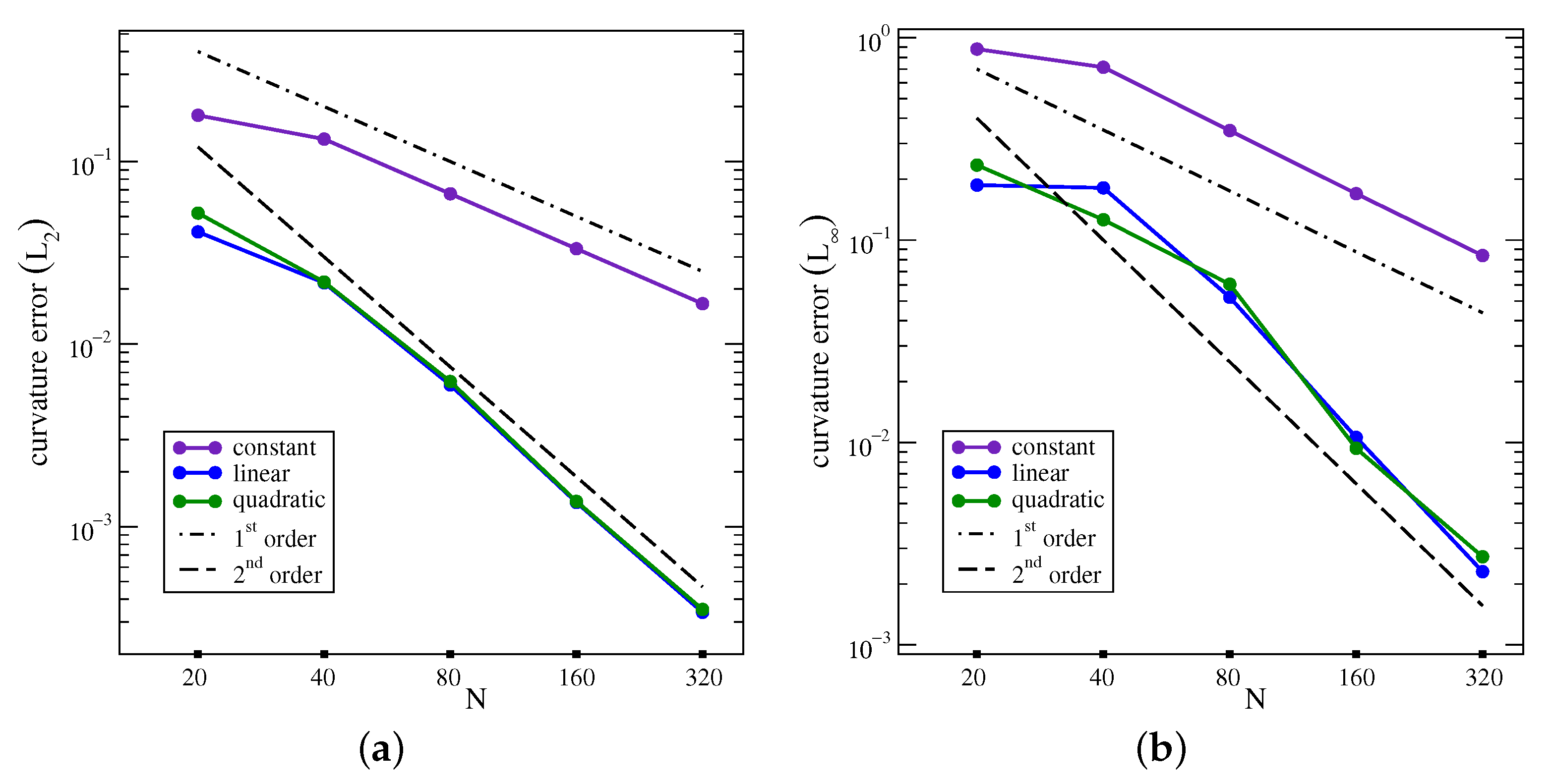
The constant approximation $P_0\left(x\right)$ is first-order-accurate in the central cell, while the linear and quadratic interpolations, $P_1\left(x\right)$ and $P_2\left(x\right)$, are both second-order-accurate. These results are a direct consequence of the fact that the three height function values $H_{-1}$, $H_0$, and $H_{+1}$ are second-order-accurate.

In place of the height function values, we can consider three consecutive values of the first derivative and of the curvature, both of them defined in Equation (3), to recompute the coefficients a, b, and c of the polynomial approximations. For the first derivative, we find

$$\begin{array}{cc}\hfill f^{\left(1\right)}\left(x\right)-P_0\left(x\right)& =\gamma f^{\left(2\right)}\left(x_m\right)h+\mathcal{O}\left(h^2\right)\hfill \\ \hfill f^{\left(1\right)}\left(x\right)-P_1\left(x\right)& ={\displaystyle \frac{12{\gamma }^2-5}{24}}{f}^{\left(3\right)}\left(x_m\right)h^2+\mathcal{O}\left(h^3\right)\hfill \\ \hfill f^{\left(1\right)}\left(x\right)-P_2\left(x\right)& =-{\displaystyle \frac{5}{24}}{f}^{\left(3\right)}\left(x_m\right)h^2+\mathcal{O}\left(h^3\right)\hfill \end{array}$$

(11)

and for the curvature

$$\begin{array}{cc}\hfill \kappa \left(x\right)-P_0\left(x\right)& ={\displaystyle \frac{\gamma S\left(x_m\right)f^{\left(3\right)}\left(x_m\right)-3\gamma f^{\left(1\right)}\left(x_m\right){\left(f^{\left(2\right)}\left(x_m\right)\right)}^2}{S^{5/2}\left(x_m\right)}}h+\mathcal{O}\left(h^2\right)\hfill \\ \hfill \kappa \left(x\right)-P_1\left(x\right)& ={\displaystyle \frac{V(\gamma ,x_m)}{8S^{7/2}\left(x_m\right)}}{h}^2+\mathcal{O}\left(h^3\right)\hfill \\ \hfill \kappa \left(x\right)-P_2\left(x\right)& ={\displaystyle \frac{-S\left(x_m\right)f^{\left(4\right)}\left(x_m\right)+5T\left(x_m\right)}{8S^{5/2}\left(x_m\right)}}{h}^2+\mathcal{O}\left(h^3\right)\hfill \end{array}$$

(12)

where $V(\gamma ,x_m)=12{\gamma }^2(4{\left(f^{\left(1\right)}\left(x_m\right)\right)}^2-1){\left(f^{\left(2\right)}\left(x_m\right)\right)}^3-(36{\gamma }^2-5)S\left(x_m\right)T\left(x_m\right)+(4{\gamma }^2-1)S^2\left(x_m\right)f^{\left(4\right)}\left(x_m\right)$. For both geometrical properties, we find again that the constant approximation is first-order-accurate, while the linear and quadratic approximations are second-order-accurate.

2.2. The Discrete Height Function

In a computational domain in two dimensions, partitioned with square cells of side h, the volume fraction field C is initialized with the new version of the Vofi library [26], which requires a user-defined function $g\left(\mathbf{x}\right)$. The interface is described by the implicit equation $g\left(\mathbf{x}\right)=0$ and points inside the reference phase satisfy $g\left(\mathbf{x}\right)<0$, while $g\left(\mathbf{x}\right)>0$ in the secondary phase. The library computes the interface intersections with the grid lines and in each cut cell performs, where required, a 1D Gauss–Legendre integration with a variable number of nodes to calculate the area between the interface line and the cell boundary. The new version optimizes the algorithms described in [27] while introducing a few new features as well. The volume fraction distribution in a $3\times 3$ block of square cells is shown in Figure 1a.

A grid cell $(i,j)$ cut by the interface will have $0<C_{i,j}<1$; then the discrete height H can be calculated with a one-dimensional (1D) stencil by adding the C data columnwise, along the y direction, or rowwise, along the x direction. Let us consider only the vertical direction, where the interface line can be locally written in the explicit form $y=f\left(x\right)$. Then,

$$\begin{array}{c}\hfill H={\displaystyle \frac{1}{h}}{\int }_{x_i-h/2}^{x_i+h/2}f\left(x\right)\mathrm{d}x={\displaystyle \frac{1}{h}}\sum _{k=-n}^n{C}_{i,j+k}{h}^2.\end{array}$$

(13)

For the volume fraction distribution of Figure 1a, three vertical heights can be computed, as shown in Figure 1b.

In the standard height function method (SHF), a fixed value of n is used; then, the 1D stencil will have 5 cells for $n=2$ and 7 cells for $n=3$. The height point H is centered in the i-th column, but it is not necessarily inside the cell $(i,j)$. Furthermore, it is not guaranteed that the interface line crosses the entire column within the stencil, or there can be more than one interface section in the given stencil. This second situation may happen in the case of complex topologies, such as droplet merging or filament breakup.

The generalized height function method (GHF) considers an adaptive 1D stencil [5], centered on the mixed cell $(i,j)$ and with a maximum length of $n_c$ cells. The algorithm is dynamical, and the summation in (13) stops as soon as a full cell, $C=1$, and an empty one, $C=0$, are found on opposite sides of the stencil. We usually consider a stencil with $n_c=5$ cells; then the height in the first two cases of Figure 3 is correctly computed, but not in Figure 3c as the stencil is not wide enough. However, in Figure 3c, the height can be computed along the x coordinate direction. In Figure 3d, there is an empty cell between the two interface sections, and the GHF method is capable of computing the two local heights; this is not the case for the SHF method. If the two sections approach each other even more and the empty cell disappears, both methods fail to provide an adequate height function value.

The height H is stored as an offset from the cell center, together with a positive integer flag to indicate if the height is measured from the top or the bottom of the cell. Therefore, when we collect the heights to compute the interface geometrical properties, we need to normalize their value to a common base of the central column before computing the numerical derivatives. In the mixed cells with no height, the integer flag is set to a negative value to indicate that an interpolation of the local geometrical data is required in that cell.

At small grid resolutions, it is not always possible to collect three consecutive values of the height function that have been computed along the same coordinate direction. In that case, we can combine discrete heights computed columnwise and rowwise. This part of the algorithm has been discussed in [22]. In this study, we investigate only the asymptotic behavior of the height function method. In the present implementation of the algorithm, a first sweep across the computational domain is required to compute the discrete heights with Equation (13); then, a second sweep is performed to numerically calculate the geometrical properties of the interface with Equation (3). This procedure is similar to what has been implemented in other numerical codes. However, the geometrical data are no longer local, but need to be stored in matrices, and with a third sweep are interpolated where necessary with the polynomials of Equations (11) and (12), after the evaluation of the interface intersections with the grid lines using Equation (9).

3. Numerical Results

3.1. Analytical Test Case

To recover numerically the theoretical results of the previous section, we consider an interface line that requires the use of the height function along both coordinate directions that is characterized by a variation of the curvature value both in magnitude and sign and where the curvature can also be computed analytically. To this end, we consider the 4-petaled star that was introduced in [20], with parametric equations

$$\begin{array}{cc}\hfill x\left(\theta \right)& =\left(R_s+A_{s}cos\left(n_s\theta \right)\right)cos\left(\theta \right)\hfill \end{array}$$

(14)

$$\begin{array}{cc}\hfill y\left(\theta \right)& =\left(R_s+A_{s}cos\left(n_s\theta \right)\right)sin\left(\theta \right)\hfill \end{array}$$

(15)

where $R_s=1$ is the radius of the base circle, $A_s=0.25$ the amplitude of the oscillation, and $n_s=4$ the number of oscillations (or petals). The interface line is drawn in Figure 4a. However, because of the symmetry of the figure, we consider only the portion of the line in the top-right quadrant where the angle $\theta$ varies in the range $[0,\pi /2]$. The straight line $\theta =\pi /4$ is another axis of symmetry, as also pointed out by the numerical results. We subdivide the square domain of side $L=R_s+A_s=5/4$ with square cells of side $h_i=R_s/N_i$, where $N_i$ is the grid resolution. The coarsest resolution is $N_0=20$, i is the resolution level, $i=0,1,\dots ,5$, and $N_i=2^i{N}_0$. A small portion of the computational grid at the lowest resolution $h_0=1/N_0$ is also shown in Figure 4a.

If the height function is numerically computed with Equation (13) along the vertical direction y, we are approximating with the first one of Equation (3) the first derivative $f^{\left(1\right)}\left(x\right)=dy/dx$ at position x with centered finite differences. Given the parametric representation of Equations (14) and (15) of the interface line, and with the notation $\dot{y}=dy/d\theta$ and $\ddot{y}=d^{2}y/d{\theta }^2$, we compute analytically the required derivatives as

$$\begin{array}{c}\hfill f^{\left(1\right)}\left(x\right)={\displaystyle \frac{dy}{dx}}={\displaystyle \frac{dy/d\theta }{dx/d\theta }}={\displaystyle \frac{\dot{y}\left(\theta \right)}{\dot{x}\left(\theta \right)}},f^{\left(2\right)}\left(x\right)={\displaystyle \frac{d}{dx}}\left({\displaystyle \frac{dy}{dx}}\right)={\displaystyle \frac{\dot{x}\ddot{y}-\dot{y}\ddot{x}}{{\dot{x}}^3}}\end{array}$$

(16)

and then the curvature as

$$\begin{array}{c}\hfill \kappa \left(x\right)={\displaystyle \frac{\dot{x}\ddot{y}-\dot{y}\ddot{x}}{{\left({\dot{x}}^2+{\dot{y}}^2\right)}^{3/2}}}.\end{array}$$

(17)

These derivatives are computed at the abscissa $x_k$ of the midpoint of the different columns, $x_k=(k-1/2)h_i$ with $k=1,2,\dots ,5N_i/4$. In the top-right quadrant of Figure 4a, Equation (14) is strictly monotonic and can be numerically inverted to express the angle $\theta$ as a function of x.

In a similar manner, we can compute analytically the derivatives of the inverse function $x=f^{-1}\left(y\right)$ at the ordinate $y_k$ and plot them as a function of the angle $\theta$ after the inversion of Equation (15). Therefore, we can plot the first derivatives $dy/dx$ and $dx/dy$ as a function of the angle $\theta$ on the same figure, as shown in Figure 4b. The sections represented with solid lines are those where the first derivative of $f\left(x\right)$ and of $f^{-1}\left(y\right)$ are smaller than one in absolute value. In the figure, we observe three consecutive switches from one representation of the derivative to the other one. In Figure 4c, we plot the second derivative and in Figure 4d the curvature, which is a geometrical property of the line that does not depend on the analytical representation.

3.2. Pointwise Convergence

The minimum radius of curvature $r_{min}$, or the maximum curvature ${\kappa }_{max}$, is found at $\theta ={\theta }_c=\pi /4$, where $r_{min}={\kappa }_{max}^{-1}\approx 3.46h_0$. At that point, the absolute value of the first derivative is equal to one, and there is a switch in the representation of the first derivative. For these two reasons, the error of the numerical approximation of the curvature is expected to be maximum. In Figure 5a, we consider three consecutive columns, the middle one centered at the abscissa $x_c=x\left({\theta }_c\right)$, computed from Equation (14). The value H of the three heights is calculated with the Vofi library and the numerical first derivative and curvature with Equation (3). The local error $E_c$ for a geometrical property q is defined as follows:

$$\begin{array}{c}\hfill E_c=|q_{n,i}-q_c|\end{array}$$

(18)

where $q_c$ is the analytical value at ${\theta }_c$ and $q_{n,i}$ the numerical value at resolution level i. The thickness of the largest column is $h=1/40$, corresponding to level $i=1$; that of the most slender one is $h=1/640$ of level $i=5$.

We also consider a $3\times 3$ block of square cells of side h of the computational domain that was previously defined. The point of interest at ${\theta }_c$ is always contained in the central column of the block, as shown in Figure 5b for the first three grid resolutions. The midpoint $x_i$ of the central column provides an approximation of the abscissa $x_c$, and it coincides with the root approximation of $x_c$ given by the bisection method. The sequence $\left\{x_i\right\}$ of midpoints is then approaching the value $x_c$ with the linear convergence of the bisection algorithm. In this case, we can define two local errors:

$$\begin{array}{c}\hfill E_{gc}=|q_{n,i}-q_c|,E_{gi}=|q_{n,i}-q_{a,i}|\end{array}$$

(19)

where $q_{n,i}$ is the numerical value of q at $x_i$ from the three heights in the block and $q_{a,i}$ is the analytical value at $x_i$. The results for the first derivative and the curvature at ${\theta }_c$ are shown in Figure 6. A second-order convergence is observed for the three different local errors, even if the sequence $\left\{x_i\right\}$ converges only linearly to $x_c$. The fluctuation in the values of $E_{gc}$ and $E_{gi}$ is due to the fact that the error is maximum at $x_c$ and that the point $x_i$ can get very close to $x_c$ at any grid spacing h and then moves away at the next refinement, as typical of the bisection method.

3.3. Convergence to the Interface Line

In Figure 4, we plot the interface line, its first and second derivatives, and the curvature as a function of the angle $\theta$. Sections of the different lines are drawn as solid lines where the first derivative of the function $f\left(x\right)$ or of the inverse function $f^{-1}\left(y\right)$ are smaller than or equal to 1 in absolute value. In these sections, we compute the error $E_k$ at the abscissa $x_k$ or ordinate $y_k$, where the height function is defined, for any geometrical property q as

$$\begin{array}{c}\hfill E_k=|q_{n,k}-q_{a,k}|\end{array}$$

(20)

where $q_{n,k}$ is the numerical value computed from the height function field and $q_{a,k}$ the corresponding analytical value. As we double the grid resolution from $N_i$ cells to $N_{i+1}=2N_i$, the number of heights along each coordinate direction also roughly doubles. To keep that number more or less constant in a plot, we divide that number by the factor $2^i$, where i is the resolution level that was previously defined. Similarly, for a second-order convergence, the error $E_k$ of Equation (20) should decrease by the factor 4 from one resolution level to the next one. Again, to keep that value more or less constant at each abscissa $x_k$, or ordinate $y_k$, we multiply it by the factor $4^i$, $E_k^{*}=4^i{E}_k$. In Figure 7, we plot the error $E_k^{*}$ of the height function, of its first and second derivatives, and of the curvature as a function of the angle $\theta$. In Figure 7a, the three switches from one representation of the interface line to the other are seen as cusps. The error is maximum at $\theta ={\theta }_c=\pi /4$, as previously anticipated. In the other plots, the error is still continuous at $\theta =\pi /4$, because of the symmetry of the interface line with respect to that axis, but not in the other two transitions. A few minima appear in the plots that are due to error cancellation for the corresponding values of the angle $\theta$.

The error of the height function model for any geometrical property q can be evaluated by the $L_2$ norm defined as

$$\begin{array}{c}\hfill E_2=\sqrt{{\displaystyle \frac{{\sum }_{k=1}^{M_i}{\left(q_{n,k}-q_{a,k}\right)}^2}{M_i}}}\end{array}$$

(21)

and by the $L_{\infty }$ norm:

$$\begin{array}{c}\hfill E_{\infty }=\underset{k}{max}|q_{n,k}-q_{a,k}|\end{array}$$

(22)

where again $q_{n,k}$ is the numerical value from the height function field, $q_{a,k}$ the analytical value at the same position $x_k$, or $y_k$, and $M_i$ the total number of cells where the height is positioned, at resolution level i.

The results for the two error norms are presented in Figure 8 for the first derivative and curvature. A second-order convergence is observed for both norms and geometrical properties.

3.4. Data Interpolation

The numerical results obtained in the previous section agree with the theoretical development of Section 2.1, namely, that the discrete height function approximation, given by Equation (13), and the numerical approximation of its geometrical properties, given by Equation (3), are second-order-accurate at the points where the height H is positioned. The vertical heights of Figure 2a are along the midline of each column. However, if the interface section inside the column crosses a horizontal grid line, as shown in Figure 2b, the two subsections of the interface lie on different grid cells. The issue is now which value should be considered for the normal vector and for the local curvature in the two subsections.

In Figure 2a, a translation of the interface line parallel to itself along the vertical direction changes the value of the three heights H by the same amount, and also the position of the intersection point with the horizontal grid line in Figure 2b. However, the values of the first and second derivatives and the curvature do not change. Therefore, to simplify the derivation, in the columns or rows where the height function is located, we consider the subgrid spacing $h_s=h/10$ and the positions at $\pm j{h}_s$, with $j=1,2,3,4$, for a total of 8 points, where we compute the error between an analytical value and that given by the numerical interpolation.

Figure 9a shows the constant, linear, and quadratic approximations of the interface line calculated from three consecutive heights H, in the vertical column with the abscissa x in the range $[0.15,0.20]$ at the coarsest resolution, $h=1/N_0$. The endpoint of the height H is always positioned in the convex region of the interface line, and the quadratic interpolation lies entirely in the same set. The central part of the linear approximation is also in the convex region. Still, it crosses the interface line, and the two endpoints of the linear interpolation are in the concave region. This implies that the linear interpolation is closer to the interface line than the quadratic one in a relevant fraction of the column size. The two interpolations are then comparable, and in any cut cell the “best” choice could be different according to the position of the intersection point $z_0$ and of the two midpoints $x_1$ and $x_2$ of Figure 2b. Figure 9b shows the constant, linear, and quadratic approximations of the interface curvature in the same column. The two interpolations are both in the convex region, and the quadratic one is somewhat closer to the analytical value. We can conclude that the linear and quadratic interpolations show a similar behavior, since the geometrical properties q, which have been computed numerically, are only second-order-accurate and outperform the constant approximation.

To be more quantitative, at each refinement level i, we have $8M_i$ additional points where we compute the errors, $M_i$ being the total number of cells with the height H. We consider the same two error norms of Equations (21) and (22), where $q_{a,k}$ is again the analytical value of the geometrical property q computed at the additional points. In contrast, the numerical value $q_{n,k}$ is now evaluated with one of the three polynomial interpolations of Equation (9). The coefficients a, b, and c are calculated from three consecutive values of q, as illustrated in Equation (8) for the height function. Figure 10 and Figure 11 show the convergence of $L_2$ and $L_{\infty }$ error norms for the interpolation of the first derivative and of the curvature, respectively. These results agree with the theoretical ones of Equations (11) and (12). The constant approximation shows first-order convergence. This is by far the most commonly used approximation in two-phase flow simulations with the one-fluid formulation of the Navier–Stokes equations. The linear and quadratic interpolations compute the first derivative more accurately with second-order convergence. This interpolation should be used at any grid resolution only when the interface line intersects a horizontal grid line in a given vertical column, as shown in Figure 2b, but not, for example, in the two adjacent columns. For the interpolation, a few more computations need to be performed: geometrical data need to be collected from the two lateral columns (or rows) to approximate the intersection $z_0$ and the position of the two midpoints $x_1$ and $x_2$, where the geometrical data need to be interpolated. In a local Cartesian coordinate system with the origin on the bottom-left corner, the abscissas of the two midpoints are $x_1=z_0/2$ and $x_2=(h+z_0)/2$, respectively.

4. Conclusions

In this study, we considered the height function (HF) method for the representation of an interface line and the calculation of its geometrical properties. We proposed a numerical algorithm that removes the inconsistency between the theoretical and numerical results presented in many papers: the HF method is observed to have first-order convergence with grid refinement while theoretical results indicate second-order convergence. The HF method integrates the volume fraction (VOF) field along a column of grid cells of a Cartesian grid and provides a smoother field to be differentiated with finite differences. We chose the generalized height function (GHF) approach, which considers an adaptive stencil for the VOF function integration, over the standard height function (SHF) approach, which considers a fixed stencil, because it computes more accurate heights, in particular in high-curvature regions.

With the HF values from three consecutive columns of cells along the same coordinate direction and centered finite differences, the first and second derivatives of the interface line can be computed with second-order convergence with grid refinement. The unit normal $\mathbf{n}$ and the curvature $\kappa$ are then calculated along the column midline from these two derivatives. The interface line can intersect more than one cell in a given column of a Cartesian grid. When this happens, the interface geometrical properties have to be interpolated in the cut cells from the value in the column midline. We considered three polynomials that corresponded to constant, linear, and quadratic approximations of the interface line inside the column, respectively. The constant approximation is the most widely used approximation and provides first-order convergence, while the linear and quadratic approximations provide second-order convergence.

Finally, we considered an interface line in a uniform Cartesian grid. The interface is described by differentiable parametric equations and is characterized by a curvature changing both in magnitude and sign. The numerical results are in agreement with the theory presented.

The HF method has been extended to three dimensions [5,28]. If the interface section in a column is shared by two consecutive cubic cells, the two midpoints $x_1$ and $x_2$ of Figure 2b in 2D become the barycenters of two interface subsections. Expressions for the barycenter coordinates have been derived for a linear interface cutting a cubic cell [12]; this task becomes much more complicated for a quadratic interface and probably will require some approximations. Therefore, the linear interpolation should be considered in practice, as it provides second-order convergence with grid refinement at a lower computational cost. We believe that this algorithm may enhance robustness and limit phase break-up caused by improper surface tension evaluation in small structures. We plan to test this numerical algorithm in three dimensions and implement it in dynamic codes to evaluate its robustness.