CFD-Assisted Design of an NH₃/H₂ Combustion Chamber Based on the Rich–Quench–Lean Concept

Abstract

Ammonia (NH₃) and hydrogen (H₂) are considered promising fuels for the power sector’s decarbonization. Their combustion is capable of producing energy with zero direct CO₂ emissions, and ammonia can act as a stable energy H₂ carrier. This study numerically investigates the design and implementation of staged combustion of a mixture of NH₃/H₂ by means of CFD simulations. The investigation employed the single-phase flow RANS governing equations and the eddy dissipation concept (EDC) combustion model, with the incorporation of a detailed kinetic mechanism. The combustion chamber operates under the RQL (rich–quench–lean) combustion regime. The first stage operates under rich conditions, firing mixtures of ammonia in air, enriched by hydrogen (H₂) to enhance combustion properties in a swirl and bluff-body stabilized burner. The secondary stage injects additional air and hydrogen to mitigate unburnt ammonia and NO_x emissions. Simulations of the first stage were performed for a thermal input ranging from 4 kW to 8 kW and flames with an equivalence ratio of 1.2. In the second stage, additional hydrogen is injected with a thermal input of either 1 kW or 2 KW, and air is added to adjust the global equivalence ratio to 0.6.

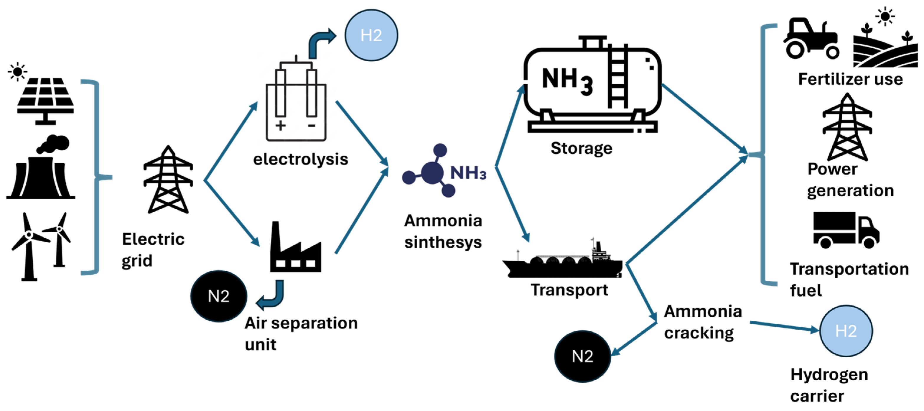
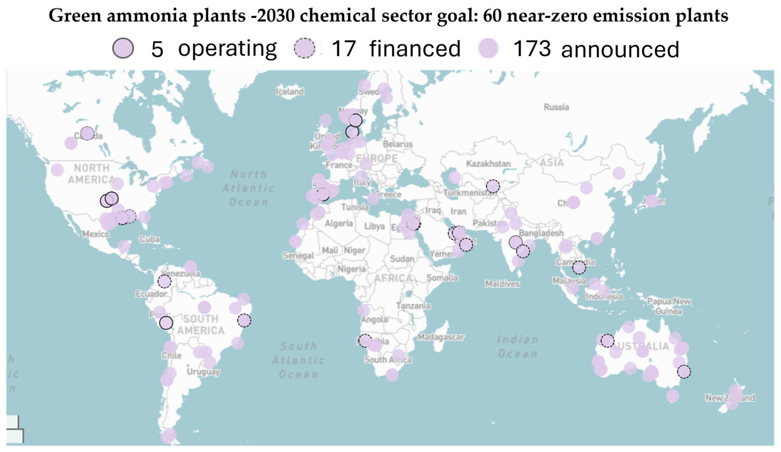
1. Introduction

The climate change effect on our planet has raised concerns about how our society produces energy and its impact on the environment in terms of pollution and global warming. The only way to tackle this problem is by implementing cleaner energy production technologies that enable sustainable fuel implementation and reduce our dependence on fossil fuels. Recent events, such as the global pandemic and geopolitical instabilities, have raised concerns regarding the robustness and vulnerability of logistical chains and energy dependence on external sources. The production of sustainable fuels and the use of energy carriers are necessary to meet the emissions reduction set by the Paris Agreement in order to keep the average global temperature below 2 °C by the end of the century [1] and further improve energy independence.

Ammonia (NH₃) is emerging as a promising carbon-free energy carrier due to its high hydrogen content, existing infrastructure, and relevance for hard-to-abate sectors such as power, industry, and maritime transport. As one of the most produced chemicals globally (183 Mt in 2020) [2], it plays a key role in fertilizer production and other industrial applications [3]. Current ammonia production is highly carbon-intensive, primarily based on fossil fuels, and results in approximately 2.4 tons of CO₂ per ton of ammonia, significantly more than steel or cement production [4]. However, ammonia can also be synthesized from green hydrogen produced using renewable electricity and water, enabling the creation of a sustainable, carbon-free fuel. As illustrated in Figure 1, green ammonia production and distribution pathways are being actively developed, with initiatives such as green maritime corridors aiming to link ammonia produced in southern Europe with northern European ports [5,6,7].

Figure 2 shows that numerous green ammonia projects are underway globally, with recent announcements indicating that projected capacity could exceed 2030 targets. Notably, around 30% of the required capacity is already financed, reflecting a strong commitment from both the public and private sectors. The recent commitment from both private and governmental parties highlights the increased interest in green ammonia, and a green transition pathway is already being carved, considering the projected demand for green ammonia [9].

Ammonia is a promising alternative fuel with a lower heating value of 18.8 MJ/kg, comparable to methanol with 19.7 MJ/kg [11]. While it has a lower energy density than hydrogen by mass, its ease of storage as a liquid under moderate pressure gives it a higher volumetric energy density of 11.5 MJ/L than both liquid and compressed hydrogen [12,13]. The combustion of ammonia offers a carbon-free solution, though its low flame speed and high ignition energy pose challenges for stable and efficient combustion [6,7,14,15].

These aforementioned considerations and findings led to the development and investigation of a modular laboratory-scale staged combustion chamber to evaluate different air–fuel mixing strategies, equivalence ratios, and fuel mixtures. One of the key benefits of a modular design is its flexibility in testing different combustion configurations. By allowing researchers to modify components such as burner geometry, fuel injection systems, and airflow patterns, a modular chamber enables the study of various combustion regimes and operating conditions without requiring a complete redesign. This adaptability is particularly useful for conducting parametric studies and optimizing combustion performance while minimizing emissions.

Figure 3 illustrates the air and fuel injection strategy. Although it is not a true RQL configuration, as it lacks the quick-mixing/quick-quench stage, the rich–lean approach has proven to be a successful solution for NO_x mitigation. Additionally, it includes a secondary fuel injection that improves combustion stability during the second stage of operation and mitigates N₂O production, which is associated with incomplete and low-temperature ammonia combustion.

The literature strongly supports the motivation for the selection of the RQL strategy. Rodolfo et al. [15] evaluated different combustion concepts for stationary gas turbines operating with ammonia, including RQL, dry low emissions (DLE), and moderate or intense low oxygen dilution (MILD) strategies through the use of chemical reactor networks. Their findings indicated that RQL provides the best compromise between flame stability and emissions control. The study also noted that H₂ formed in the rich stage significantly aids downstream combustion in the lean zone, making RQL an attractive solution for staged ammonia combustion.

Experimental evidence further supports this approach. Okafor et al. [16] performed experimental and numerical investigations of staged combustion using NH₃/air and NH₃/CH₄/air mixtures, demonstrating that swirl-stabilized flames enhance combustion stability and reduce NO_x and unburned ammonia emissions. Their results indicated that achieving a homogeneous air–fuel mixture in the primary zone is critical for maintaining combustion efficiency and controlling emissions. They also highlighted the sensitivity of ammonia flames to equivalence ratio variations. Additionally, Kurata et al. [17] developed and demonstrated an RQL-type combustor for a 50 kW micro gas turbine system operating with NH₃/CH₄ blends.

Numerical investigations of ammonia combustion have employed different modeling approaches ranging from simplified reactor networks to comprehensive CFD simulations [15,18,19]. These studies aim to gain an understanding of the fundamental physics, validate kinetic mechanisms, and identify optimal combustion strategies to enhance efficiency while minimizing pollutant emissions. Validated chemical kinetics mechanisms, such as the Konnov mechanism [20] and reduced variations [15,21,22,23], have been fundamental in accurately modeling ammonia combustion under various conditions and understanding phenomena such as NO_x and N₂O formation, NH₃ dissociation into H₂ under rich regimes, and flame stabilization.

To address ammonia’s inherently poor combustion properties, researchers have blended ammonia with more reactive fuels, such as H₂ or CH₄, which have been shown to significantly improve flame stability, enhance ignition properties, and expand the flammability range, facilitating more robust combustion strategies. Studies indicate that blending ammonia with 10–50% hydrogen by volume can increase reactivity and reduce unburned ammonia emissions, although raising the potential of NO_x formation due to higher flame temperatures [24,25]. These findings reinforce the need for optimization studies focusing on mixing ratios and operating conditions.

CFD simulations utilizing Reynolds-Averaged Navier–Stokes (RANS) equations or large eddy simulation (LES) have been employed to study ammonia and ammonia/hydrogen blend combustion in single-phase [24,25,26] and multi-phase flow configurations [27], including scenarios involving liquid ammonia spray injection. Notably, several studies have demonstrated good agreement between simulations and experimental data, demonstrating the capability of current models to capture key aspects of ammonia and NH₃/H₂ combustion dynamics. The improvement in the modeling accuracy can be primarily attributed to recent advances in ammonia combustion modeling, particularly in chemical kinetics, turbulence–chemistry interactions, and multi-phase treatment.

Based on previous findings and works from the literature, this work aims to propose a design for a laboratory-scale RQL combustion chamber with the aid of CFD simulations to provide insight into the combustion processes. A detailed kinetic mechanism captures the complex interactions between chemical reactions, heat transfer, and fluid dynamics within the chamber. Various geometrical configurations and firing strategies are systematically evaluated in terms of combustion efficiency, temperature distribution, and pollutant emissions. The objective is to identify the most promising design for experimental implementation, contributing to the development of cleaner and more efficient combustion technologies. The results of this study can serve as a foundation for future works where experimental measurements, such as exhaust gas analysis, temperature profiles, and chemiluminescence analysis are planned.

The structure of this paper has been organized as follows. First, the methodology, simulation parameters, and geometry used in the simulations are presented. This is followed by a detailed description of the numerical setup, including the turbulence and combustion models and mesh configuration. Finally, the results of the simulations are discussed, and the main conclusions are outlined.

2. Methodology

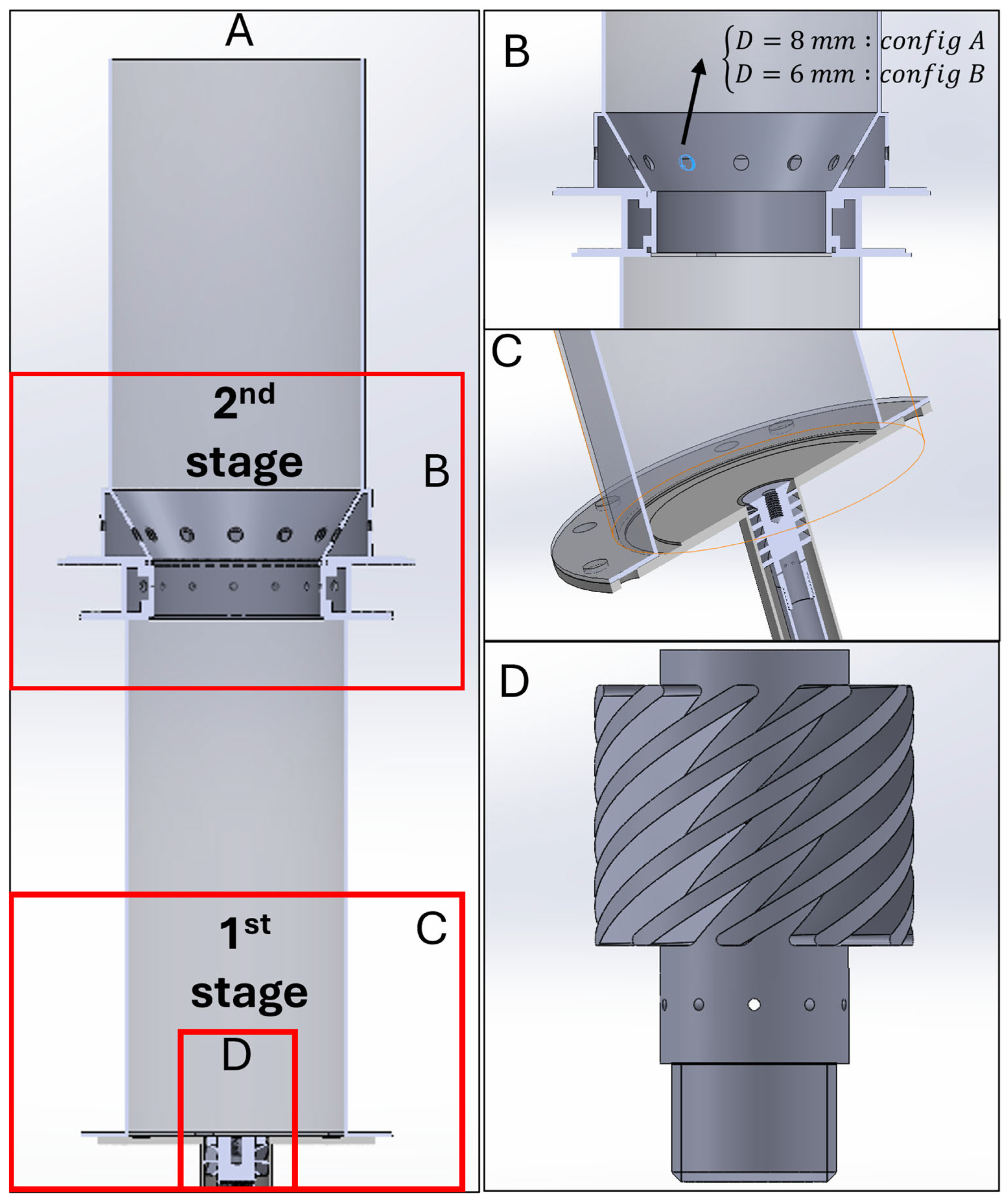
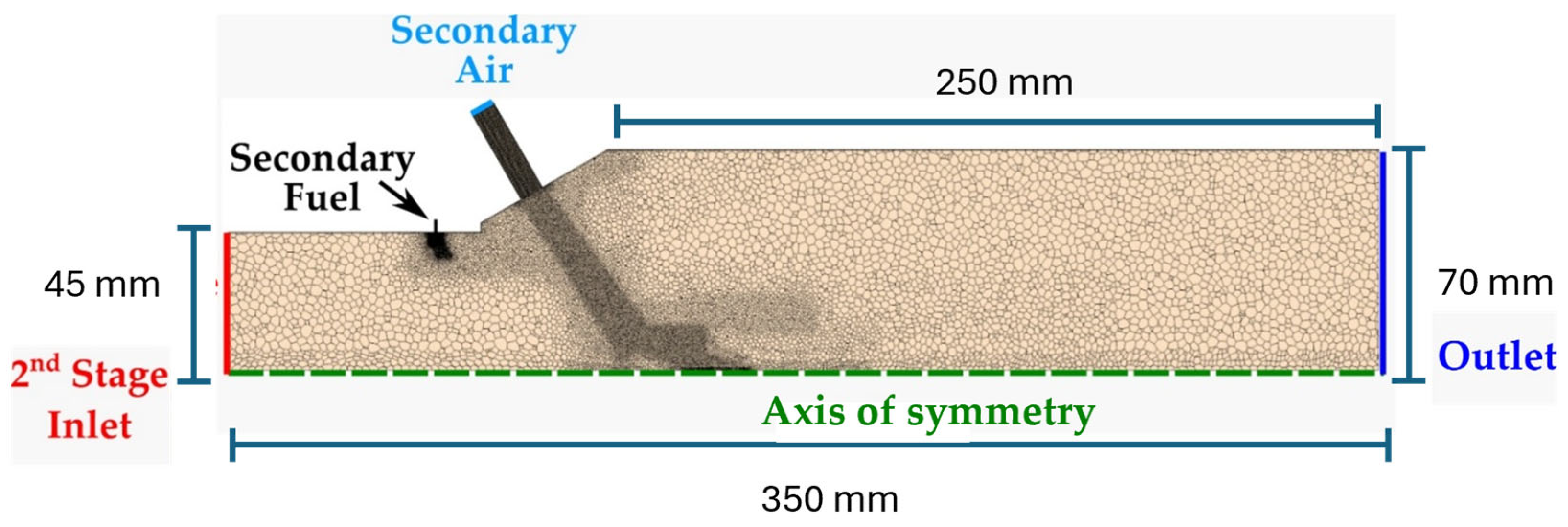
2.1. Burner Geometry

The design of the combustion chamber was based on previous works where the rich combustion of ammonia/hydrogen mixtures was investigated [20]. The first stage was developed with a similar concept, where the new burner comprises a modular design to be operated and adapted to more flexible operating conditions. The burner operates under a premixed combustion regime with a 45° swirl vane angle (SVA) swirler and a bluff body, which can be interchanged with the swirler vanes as needed. In the current design, the burner inlet is engineered to form a 2 mm annular slot, directing the reactant mixture from the swirler toward a 36 mm diameter bluff body, which promotes recirculation and enhances flame anchoring. The combustion chamber was designed with a modular architecture, allowing interchangeable swirlers and bluff body to accommodate different combustion regimes. The second stage of the combustion chamber was designed to be coupled to the first stage, which is composed of 3 different parts: fuel injection, air injection, and burner cover. Figure 4 shows the burner geometry implemented in the simulations for the first and second stages of the burner, which will be built according to the findings of the numerical studies.

2.2. Operating Conditions

In this work, different operating conditions were simulated to understand the performance and working envelope of the developed combustor. For the first stage, only the thermal input was varied in order to understand its impact on ammonia combustion efficiency and pollutant production.

Table 1. Simulation conditions for the first stage burner.

Thermal Input (kW)	Primary Equivalence Ratio	Fuel Mixture
4	1.2	80% NH3/20% H2
6	1.2	80% NH3/20% H2
8	1.2	80% NH3/20% H2

shows the different working conditions simulated for the first stage.

For the second stage, several parameters were tested to improve the complete combustion of ammonia, such as secondary fuel injection and a different secondary air injection geometry, aiming to improve the penetration of the secondary air into the combustion chamber and the mixing properties.

Table 2. Simulated conditions for burner operation, targeting optimal second stage conditions.

Case	Total Power (kW)	1st Stage Power Input 80%NH3/20%H2	2nd Stage Power Input 100% H2	Global Equivalence Ratio	Secondary Air Configuration (see Figure 4)
1	5	4	1	0.6	A
2	10	8	2	0.6	A
3	4	4	0	0.5	A
4	8	8	0	0.5	A
5	5	4	1	0.6	B
6	10	8	2	0.6	B
7	4	4	0	0.5	B
8	8	8	0	0.5	B

shows the different operating conditions simulated for the secondary stage. For all the simulations, the combustion chamber operated at ambient pressure, reflecting the operating conditions of the upcoming experimental campaign. The highest simulated thermal input corresponds to a global power input of 10 kW, and the minimum firing thermal input corresponds to 4 kW. Additionally, the mass flow rates for the inlet boundaries are given in

Table A1. Inlet Boundary Conditions—Mass Flow Rates for All Simulation Cases.

Case	Total Power (kW)	1st Stage Power Input 80%NH3/20%H2	1st Stage Inlet Mass Flow kg/s NH3xi = 0.147 H2xi = 0.0429 N2xi = 0.653 O2xi = 0.198	2nd Stage Power Input 100% H2	Secondary Fuel Mass Flow kg/s	Secondary Air Mass Flow kg/s	Global Equivalence Ratio	Secondary Air Configuration (See Figure 4)
1	5	4	1.99 × 10−4	1	7.60 × 10−7	1.33 × 10−4	0.6	A
2	10	8	3.97 × 10−4	2	1.52 × 10−6	2.65 × 10−4	0.6	A
3	4	4	1.99 × 10−4	0	0	1.33 × 10−4	0.5	A
4	8	8	3.97 × 10−4	0	0	2.65 × 10−4	0.5	A
5	5	4	1.99 × 10−4	1	7.60 × 10−7	1.33 × 10−4	0.6	B
6	10	8	3.97 × 10−4	2	1.52 × 10−6	2.65 × 10−4	0.6	B
7	4	4	1.99 × 10−4	0	0	1.33 × 10−4	0.5	B
8	8	8	3.97 × 10−4	0	0	2.65 × 10−4	0.5	B

, presented in Appendix A. These power inputs were selected because they are the expected experimental conditions on a laboratory scale to be tested in the near future after the combustion chamber is fully developed.

3. Numerical Methods

3.1. Governing Equations for Reactive Fluid Flow

The CFD study was performed by employing the Reynolds-Averaged Navier–Stokes (RANS) discretization. The equations are presented as follows for their compressible and conservative forms:

$${\displaystyle \frac{\mathsf{\partial }\left(\overline{\rho }\widetilde{u_j}\right)}{\mathsf{\partial }{x}_j}}=0$$

(1a)

$${\displaystyle \frac{\mathsf{\partial }}{\mathsf{\partial } x_j}}\left(\overline{\rho }\widetilde{u_j}\widetilde{u_i}\right) =-{\displaystyle \frac{\mathsf{\partial }\left(\overline{p}\right)}{\mathsf{\partial }{x}_i}} +{\displaystyle \frac{\mathsf{\partial }}{\mathsf{\partial } x_j}}\left[u\left({\displaystyle \frac{\mathsf{\partial }\widetilde{u_i}}{\mathsf{\partial }{x}_j}}+{\displaystyle \frac{\mathsf{\partial }\widetilde{u_i}}{\mathsf{\partial }{x}_j}}\right)-{\displaystyle \frac{2}{3}}u{\displaystyle \frac{\mathsf{\partial }\widetilde{u_k}}{\mathsf{\partial }{x}_k}}{\delta }_{ij}-\overline{\rho }\widetilde{u_j^{″}{u}_i^{″}}\right]+ \overline{f_b}$$

(1b)

$$\begin{array}{c}{\displaystyle \frac{\mathsf{\partial }\left(\overline{\rho }\widetilde{u_j}\tilde{h}\right)}{\mathsf{\partial }{x}_j}}=\widetilde{u_j}{\displaystyle \frac{\mathsf{\partial }\overline{p}}{\mathsf{\partial }{x}_j}}+\overline{u_j^{″}{\displaystyle \frac{\mathsf{\partial }p}{\mathsf{\partial }{x}_j}}}+\overline{{\tau }_{ij}}{\displaystyle \frac{\mathsf{\partial }\widetilde{u_i}}{\mathsf{\partial }{x}_j}}+\overline{\overline{{\tau }_{ij}}{\displaystyle \frac{\mathsf{\partial }{u}_i^{″}}{\mathsf{\partial }{x}_j}}}\\ \hspace{1em}\hspace{1em}\hspace{1em}\hspace{1em}\hspace{1em}\hspace{1em}\hspace{1em}+{\displaystyle \frac{\mathsf{\partial }}{\mathsf{\partial } x_j}}\left[\overline{{\displaystyle \frac{\lambda }{c_p}}{\displaystyle \frac{\mathsf{\partial }h}{\mathsf{\partial }{x}_j}}}-{\displaystyle \sum _{i=1}^N}\left(1-{\displaystyle \frac{1}{{Le}_i}}\right)\overline{{\displaystyle \frac{\lambda }{c_p}}{h}_i{\displaystyle \frac{\mathsf{\partial }{y}_i}{\mathsf{\partial }{x}_j}}}-\overline{\rho }\widetilde{u_j^{″}{h}^{″}}\right]+\overline{S^T}\end{array}$$

(1c)

where u_j and x_j are the velocity component and the coordinate in the jth direction, respectively, ρ denotes density, and p corresponds to the pressure. The specific heat capacity at constant pressure is given by c_p, and K is the thermal conductivity of the fluid. The term τ is the viscous stress tensor, $\lambda$ is the thermal conductivity, ${Le}_i$ is the Lewis number of species i, T is the temperature, and h is the specific enthalpy (sum of sensible and chemical enthalpy). Lastly, $S^T$ represents the energy source term due to combustion and radiation [8]. These equations are based on the assumptions that the fluid is Newtonian, mass diffusion is governed by Fick’s law, the Dufour effect is negligible, and the mixture behaves as an ideal gas. The second term on the right side of Equation (1c) is usually neglected. Furthermore, the second term into the square brackets in Equation (1c) is also often neglected, assuming that the Lewis number is equal to unity for all species.

3.2. Turbulent Model: Realizable k–ϵ

In this work, all simulations were performed with the realizable k–ϵ turbulent model. This model has been successfully widely used in CFD calculations and in previous numerical works for combustion applied to predict turbulent flow [8,24]. This model is a more recent version of the standard k–ϵ model, where some of its limitations have been addressed. Accordingly, it is more reliable and enables more accurate predictions for a broader range of conditions. The model is able to account for the effect of mean rotation in a more accurate way, being more accurate for swirling flows, such as those encountered in this work. This model has already been successfully used in numerical simulations for ammonia combustion applications and follows the same methodology as previous works [8].

The model includes a modified transport equation for the turbulent dissipation rate $\epsilon$ [28] and a variable damping function Fu, which depends on both the mean flown and turbulence characteristics. This function is applied to adjust the model coefficient C_μ.

This process ensures the model satisfies the specific mathematical constraints related to normal stresses, maintaining physical consistency with turbulence behavior (realizability). The idea of using a damped C_μ is further supported by experimental investigations conducted in boundary layers. Damping C_μ reduces turbulence intensity near the wall, which enhances the accuracy of predictions regarding flow separation, drag, and overall flow behavior in boundary layers.

The transport equation for the turbulent kinetic energy, k, can be expressed as follows:

$${\displaystyle \frac{\mathsf{\partial }\left(\rho k\right)}{\mathsf{\partial }t}}+\mathsf{\nabla }\cdot \left(\rho \overline{u}k\right)=\mathsf{\nabla }\cdot \left[\left(\mu +{\displaystyle \frac{{\mu }_t}{{\sigma }_k}}\right)\mathsf{\nabla }k\right]+P_k-\rho (\epsilon -{\epsilon }_0)$$

(2)

In this equation, $\mu$ denotes the dynamic viscosity, while ${\mu }_t$ represents the turbulent viscosity. The production of turbulent kinetic energy was denoted by P_k and s_k is a model coefficient. The equation governing the dissipation rate of turbulent kinetic energy, e, is given by:

$${\displaystyle \frac{\mathsf{\partial }\left(\rho ϵ\right)}{\mathsf{\partial }t}}+\mathsf{\nabla }\cdot \left(\rho \overline{\mu }ϵ\right)=\mathsf{\nabla }\cdot \left(\left(\mu +{\displaystyle \frac{{\mu }_t}{{\sigma }_{ϵ}}}\right)\mathsf{\nabla }ϵ\right)+C_{ϵ1}{\displaystyle \frac{1}{T_e}}{P}_{ϵ}-C_{ϵ2}{F}_2\rho \left({\displaystyle \frac{ϵ}{T_e}}-{\displaystyle \frac{{ϵ}_0}{T_0}}\right)$$

(3)

where ${ϵ}_0$ is an ambient turbulence value that is included in the source term to counteract turbulence dissipation [29], ${\sigma }_{ϵ}$ is a constant of the model, and $P_{ϵ}$is the production term for the dissipation rate. The time scale $T_0$ is defined as $T_0$ = max $\left({\displaystyle \frac{k_0}{{ϵ}_0}},C_t{\displaystyle \frac{\nu }{{ϵ}_0}}\right)$, where $C_t$, $C_{{ϵ}_1}$ and $C_{{ϵ}_2}$ are empirical constants used in the model. The $F_2$ damping function is defined as follows:

$$F_2={\displaystyle \frac{k}{k+\sqrt{\nu ϵ}}}$$

(4)

Here, $\nu$ denotes the kinematic viscosity. The turbulent eddy viscosity, ${\mu }_t$, is determined using the following expression:

$${\mu }_t=\overline{\rho }{C}_{\mu }{F}_{\mu }k{T}_e$$

(5)

where $T_e={\displaystyle \frac{k}{ϵ}}$ is the large eddy time scale, while $C_{\mu }$ is a model constant, and the function $F_{\mu }$ serves as a damping factor that mimics the decrease in the turbulent mixing close to walls. This ensures the model realizability and is defined as follows:

$$F_{\mu }={\displaystyle \frac{1}{C_{\mu }\left(A_0+A_s\frac{U^{*}k}{ϵ}\right)}}$$

(6)

here, $A_0$ is a constant set to 4.0. The variable $A_s$ depends on both the strain rate and the angular velocity of the flow. $U^{*}$ represents a velocity scale that accounts for the effects of the strain and flow rotation defined as $U^{*}=\sqrt{S_{ii}{S}_{ij}+{\Omega }_{ij}{\Omega }_{ij}}$, where $S_{ij}$ represents the mean strain rate tensor and ${\Omega }_{ij}$ is the mean rate of rotation tensor. The term $A_s$ is calculated using the following set of expressions:

$$A_s=\sqrt{6}\mathit{cos}\varphi$$

(7)

here, $\varphi$ is defined as:

$$\varphi ={\displaystyle \frac{1}{3}}\mathit{arccos}\left(\sqrt{6}W\right)$$

(8)

here, $W$ is a dimensionless parameter related to the mean rate of rotation and the strain rate [30]. The values of the constants of the model are the following: ${\sigma }_k=1.0,{\sigma }_{ϵ}=1.2,C_t=1,C\mu =0.09,C_{ϵ1}=\mathit{max}\left(0.43,{\displaystyle \frac{\eta }{5+\eta }}\right),where\eta ={\displaystyle \frac{Sk}{ϵ}},and{C}_{ϵ2}=$ 1.9. These equations form the basis of the realizable k–ϵ model, enabling more accurate and reliable simulations of turbulent flows compared to the standard model over a wide range of engineering applications [31].

3.3. Chemical Kinetics Mechanism

Understanding the ammonia combustion/oxidation process for a broad region of operating conditions has been challenging for combustion kinetics and simulations. However, the recent interest in ammonia as an energy vector for combustion applications has provided a variety of experimental data for different combustion regimes and combustion strategies that allowed the development of more accurate kinetic mechanisms for a wide range of conditions and fuel blends.

The chemical kinetics model used in this work was developed by Stagni et al. [21]. The mechanism is based on previous studies by the author [21]. and was further improved by implementing a sub-mechanism based on the most recent available theoretical data [30,32,33].

The revised mechanism comprises 31 species and 203 reactions [21] and was validated against a wide range of experimental data on NH₃ pyrolysis and oxidation. This kinetic mechanism was selected for this work due to its sensitivity to the NO_x and N₂O reaction pathways, which are crucial to understanding and simulating pollutant emissions for ammonia combustion applications. The mechanism also incorporates N_xH_y reactions that significantly impact the combustion process due to the interaction of H₂ and NH₃ inside the combustion chamber. Stagni et al. [21] stated that the mechanism allowed to understand better the impact of changing from 100% NH₃ to mixtures with H₂, with the H radical from direct oxidation of H₂ enhancing reactivity. An additional update involved the thermal NO_x model, introducing the production rate recommended by Abian et al. [34].

3.4. Combustion Model

Combustion is an inherently complex process due to the flow field–chemistry interactions; hence, it becomes necessary to employ a suitable model for the problem under consideration, especially when considering the impact on computational costs [35]. STAR-CCM+ provides three turbulence–chemistry interaction models applicable to combustion simulations, which are also compatible with Reynolds-Averaged Navier–Stokes (RANS) single-phase flow calculations [36].

For this work, the model implementation was similar to what was already successfully employed in previous works with ammonia combustion using CFD simulations [8,14,37,38]. The eddy dissipation concept (EDC) model was chosen as the combustion modeling approach.

The EDC model assumes that chemical reactions primarily occur in small-scale turbulent structures with a size of the order of the Kolmogorov scale, where intense mixing leads to rapid combustion. Within these fine structures, the reactants are considered perfectly mixed, allowing combustion to proceed at a rate controlled by turbulence dissipation rather than by chemical kinetics alone. The wide range of chemical reaction time scales requires the use of an ordinary differential equation (ODE) solver capable of efficiently handling stiff reaction systems to integrate the chemical source terms accurately.

These considerations make the EDC model particularly useful for high-turbulence combustion systems, such as gas turbine combustors, industrial burners, and internal combustion engines, where turbulent mixing dominates reaction rates. The model also offers the flexibility to handle simple and detailed chemical reaction mechanisms, making it suitable for applications requiring accurate pollutant predictions, such as NO_x and N₂O formation and NH₃ dissociation. Additionally, it is efficiently coupled with turbulence models like the k–ε or k–ω approaches, allowing for a more realistic representation of turbulence–chemistry interactions. However, the model assumes that combustion is limited to fine-scale turbulent structures, which may not fully capture effects like flame quenching or stretch in low-turbulence regimes. Despite these limitations, the EDC model remains a powerful and computationally efficient tool for predicting combustion performance in practical engineering applications. Bridging the gap between turbulence modeling and chemical kinetics provides a more accurate representation of combustion processes than simpler models assuming infinitely fast chemistry.

In the EDC, the reaction rate is governed by solving the full chemical kinetic mechanism over the residence time of the fine structures and can manage a wide range of kinetic time scales present in the chemical mechanism [36]. The model requires the solution of the species transport equations, which are given by:

$${\displaystyle \frac{\mathsf{\partial }}{\mathsf{\partial }t}}\left(\mathsf{\rho }{Y}_i\right) +{\displaystyle \frac{\mathsf{\partial }}{\mathsf{\partial }{x}_j}} \left(\mathsf{\rho }{u}_j{Y}_i+F_{k,j}\right)={\mathsf{\omega }}_i$$

(9)

Y_i refers to the mass fraction of species i, and F_k,j denotes the corresponding diffusion flux. The source term ω_i accounts for the reaction rate of species i. Within the framework of the EDC model, the reaction rate ω_i of species i is expressed as follows:

$${\mathsf{\omega }}_i=\mathsf{\rho }f\left({\displaystyle \frac{Y_i^{\mathrm{*}}-Y_i}{\mathsf{\tau }}}\right)$$

(10)

here, τ represents the residence time, f is the factor that adjusts mean reaction rate, and $Y_i^{\mathrm{*}}$ is the species mass fraction calculated after time step integration [23], as indicated in Equation (13). The time scale is proportional to the Kolmogorov time scale, and f is defined as follows:

$$f= {\left({\left[C_{l1}{\left({\displaystyle \frac{v{C}_{l2}{\mathsf{\tau }}_{*}}{L_t^2}}\right)}^{0.25}\right]}^{-3} -1\right)}^{-1}$$

(11)

here, C_l1 = 2.1377 is the model constant for the fine structure length [24], L_t denotes the turbulent length scale, and ${\mathsf{\tau }}_{*}$ represents the turbulent time scale. The time scale used in Equation (11), is determined as follows:

$${\mathsf{\tau }}_{*}=C_t{\mathsf{\tau }}_{\mathsf{\eta }}$$

(12)

In this expression, C_t is a model constant typically set to the default value 0.4082, and τ_η refers to the Kolmogorov turbulent time scale, defined as $\sqrt{{\displaystyle \frac{v}{\mathsf{ϵ}}}}$. The mean species mass fraction are calculated as follows:

$$Y_i^{\mathrm{*}}= Y_i + {\int }_0^{\mathsf{\tau }}{r}_k dt$$

(13)

where r_k expresses the net reaction rate of species k, based on the respective Arrhenius expressions [23].

3.5. Radiation Model

The discrete ordinates method (DOM) [39] was employed to simulate thermal radiation in the combustion chamber. This method solves the radiative transfer equation by discretizing it into a finite set of directions, known as ordinates. Increasing the number of ordinates enhances accuracy but also increases computational demand. In this study, the S₄ quadrature was utilized for the calculations.

For the first stage simulation, the medium radiative properties were determined with the use of the k-distribution model. It accounts for the spectral dependence of the absorption coefficient of the medium due to H₂O. Spectral reordering is used to solve the radiative transfer equations for each discrete direction, spectral band, and quadrature point [40]. The model allows for an accurate and efficient numerical integration with a limited number of quadrature points. Modest and Zhang [40] later extended the concept, leading to the development of the full-spectrum k-distribution (FSK) method [41]. Today, the FSK approach is widely recognized as one of the most accurate and computationally efficient models for simulating full-spectrum radiative transfer in combustion systems [42,43,44].

This method allows a very efficient and accurate numerical integration using a limited number of quadrature points. The k-distribution model has been previously implemented in research related to ammonia combustion [38].

For the second stage simulation, thermal radiation was modeled using the discrete ordinates method (DOM) along with the weighted sum of gray gases (WSGG) model. This approach approximates spectrally integrated thermal radiation by summing the solutions of the radiative transfer equation (RTE) over a limited number of gray gases, each associated with a specific weighting factor. The model was selected due to its lower computational cost compared to other models. Previous studies have demonstrated that the WSGG model provides an efficient solution for engineering applications when appropriate parameters are applied. However, if the computational cost is not a concern, then the FSCK model generally offers higher accuracy. The WSGG model has been widely applied in combustion simulations, particularly for CO₂ and H₂O mixtures, which are the primary participating species in the combustion of hydrocarbons.

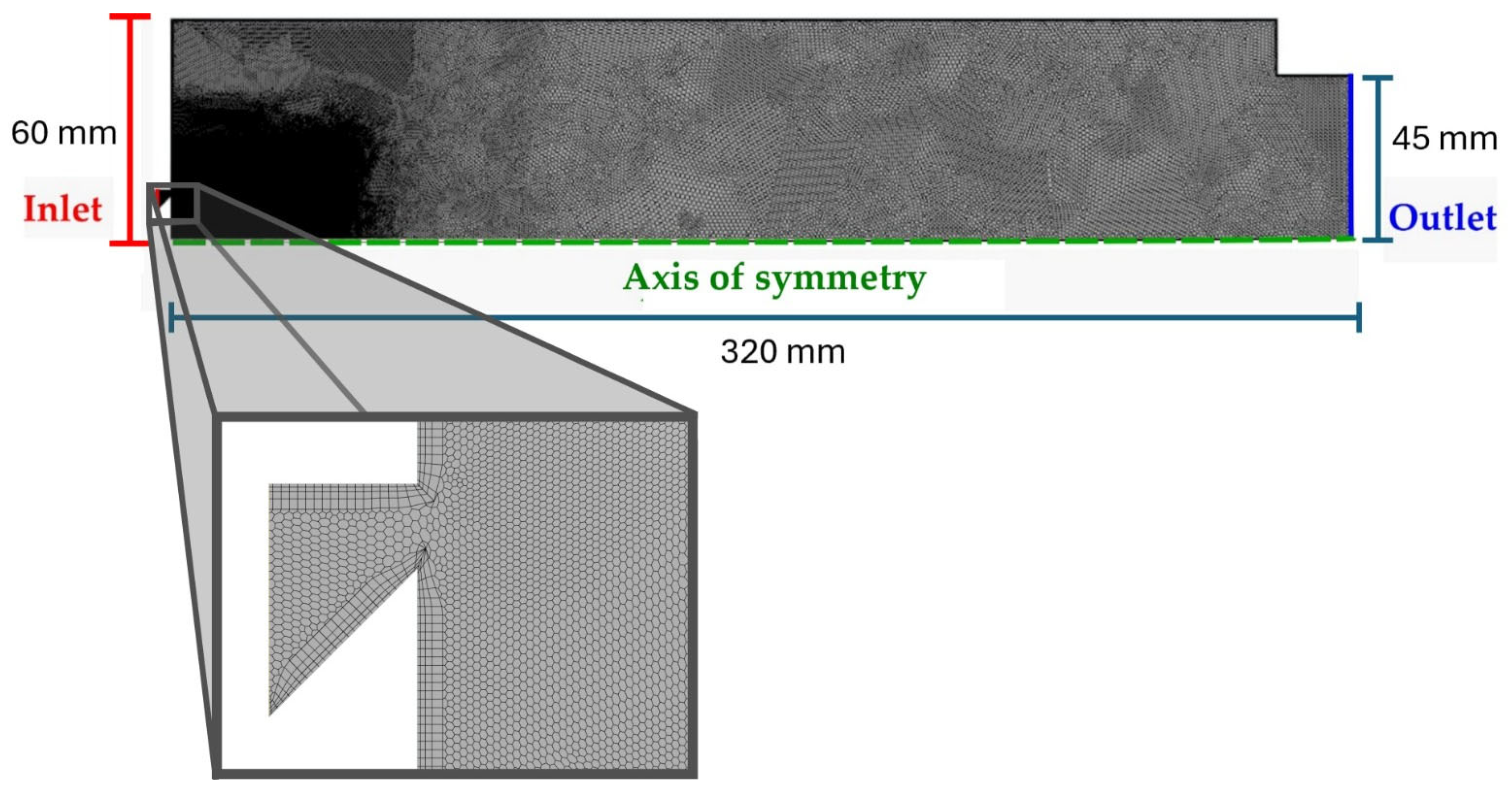
3.6. Mesh and Computational Domain

For this study, each stage of the combustion chamber was modeled independently to optimize computational efficiency and enable a parametric analysis of different combustion chamber geometries, combustion regimes, and fuel mixtures. The mesh geometry was generated using the STAR-CCM+ software package. In the first stage, a 2D axisymmetric mesh was used, while in the second stage, a 30° sector was simulated using a 3D mesh with periodic boundary conditions. A 3D simulation is needed in the second stage because the secondary air and fuel are injected through discrete holes. Hence, the axisymmetric domain cannot be implemented.

Both meshes were created with polyhedral control volumes, and a prism layer was used for the near-wall region. The meshes included local refinement to accurately predict and capture the flow field and chemistry in the flame region and inside the combustion chamber and to account for the geometric details of the combustion chamber. Figure 4 shows the burner geometry implemented in the simulations for the first and second stages of the burner, which will be built according to the findings of the numerical studies.

Figure 5 illustrates a section view for the first stage combustor and indicates the type of boundary conditions employed. Additional information on the boundary conditions is given in

Table 3. Boundary conditions for the first stage simulation.

1st stage	Momentum	Temperature
Wall	Laws of the wall	1100 K
Inlet	Mass flow inlet; Turbulence intensity = 0.1; Viscosity ratio = 10	300 K
Outlet	Pressure outlet	Extrapolated

. The first stage mesh comprises unstructured polyhedrons with sizes between 0.2 and 1 mm. The resolution of the near-wall region was fixed at 0.2 mm for the first prism layer, with a growth ratio of 1.1, creating a mesh with a total of 78 k cells.

The second stage mesh used a similar procedure with a cell base size of 2 mm, a near-wall mesh resolution of 0.2 for the prism layer, and a growth ratio of 1.1 mm, leading to 587 k cells. Figure 6 illustrates a section view of the second stage burner mesh and outlines the boundary conditions.

Table 4. Boundary conditions for the second stage simulation.

2nd Stage	Momentum	Energy
Wall	Laws of the wall	1100 K
Inlet section	Radial profile	Radial profile
Secondary Fuel inlet	Mass flow inlet, Turbulence intensity = 0.1; Viscosity ratio = 10	300 K
Species	Radial profile	Radial profile
Secondary air inlet	Mass flow inlet, Turbulence intensity = 0.1; Viscosity ratio = 10	300 K
Outlet	Pressure outlet	Extrapolated

gives additional details of the boundary conditions. The computed radial profiles of species concentration, temperature, and velocity at the exit of the first stage were applied as boundary conditions at the inlet of the second stage.

4. Results

4.1. First Stage Simulation

For the first stage, simulations were performed for three different power setups ranging from 4 to 8 kW. The simulations were performed in order to understand how the envisaged operating envelope would affect flame stability and emissions from the first stage. The burner fired a premixed fuel mixture of 80% NH₃/20% H₂ at an equivalence ratio of 1.2. Figure 7 shows the temperature contours for the three simulated conditions. The NO_x, H₂, N₂O, and NH₃ molar fraction contours for each power input can be seen in Figure 8, Figure 9 and Figure 10. Figure 11 shows the outlet radial profiles for relevant quantities that are used as inlet boundary conditions for the second stage. Additionally, the profiles can aid in understanding the operation of the combustion chamber first stage.

The maximum temperature for all simulations can be observed inside the IRZ (inner recirculation zone). For the 4 kW and 6kW cases, the flame appears to have a similar behavior. However, the flame front shifts downstream with increasing thermal power due to the corresponding rise in inlet velocities. Ammonia is especially sensitive to this phenomenon due to its inherently reduced flame speed and reactivity, leading to a narrower flammability limit. The 8 kW flame showed the impact of ammonia’s low reactivity more evidently, with the flame front propagating downstream, leading to a slight reduction to 1947 K of the peak temperature inside the IRZ. Even though the simulations predicted a stable frame and almost complete fuel oxidation, flame instabilities are expected when operating at higher power outputs due to the poor combustion characteristics of ammonia. The stability of the flames will be addressed in the near future through experimental measurement campaigns on the final designed model for a more precise definition of the operating envelope. The 8 kW simulation yielded higher outlet temperatures. This can be attributed to lower heat losses due to the reduced residence time inside the combustion chamber and because the heat losses represent a smaller fraction of the total energy output.

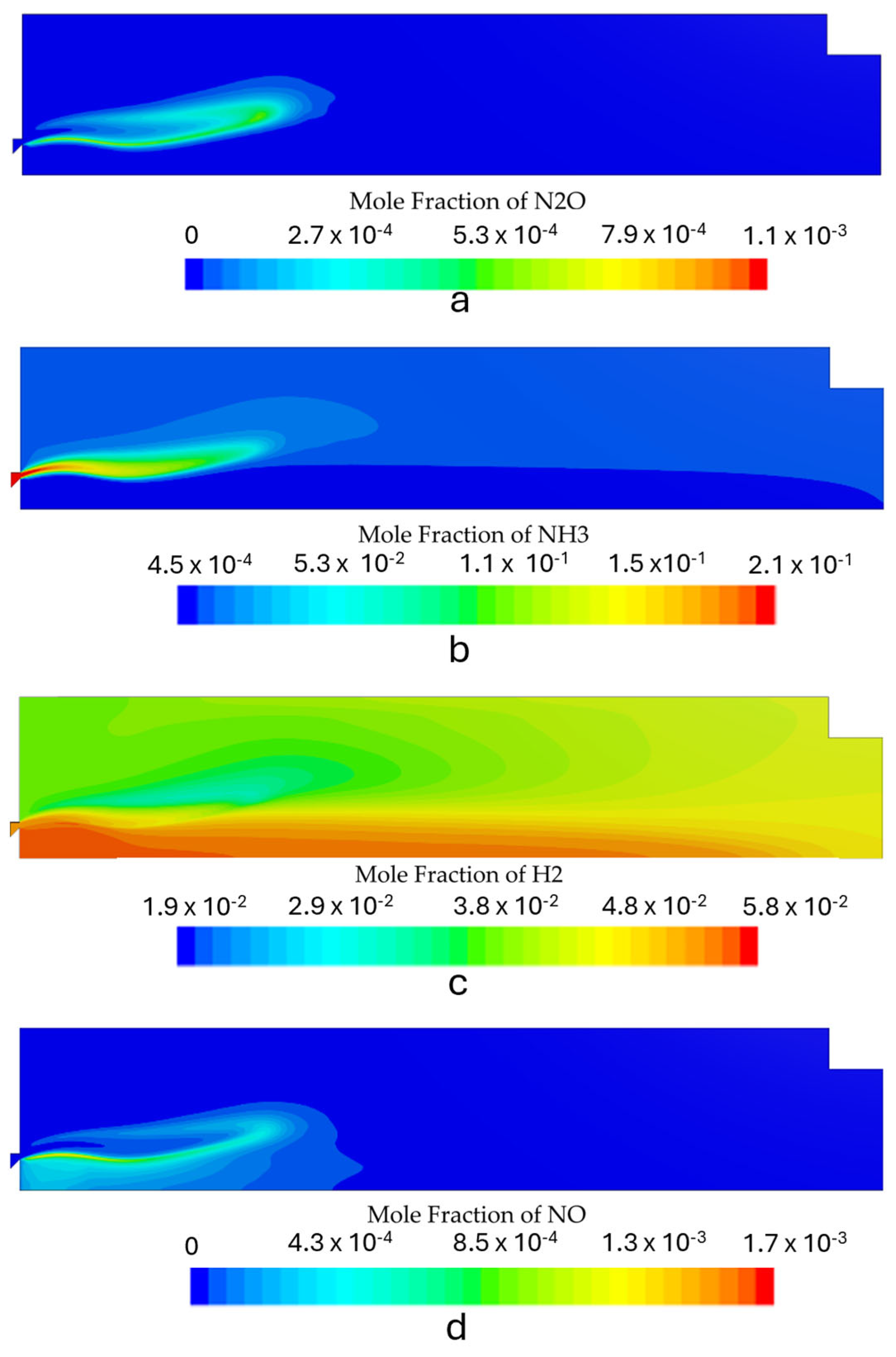
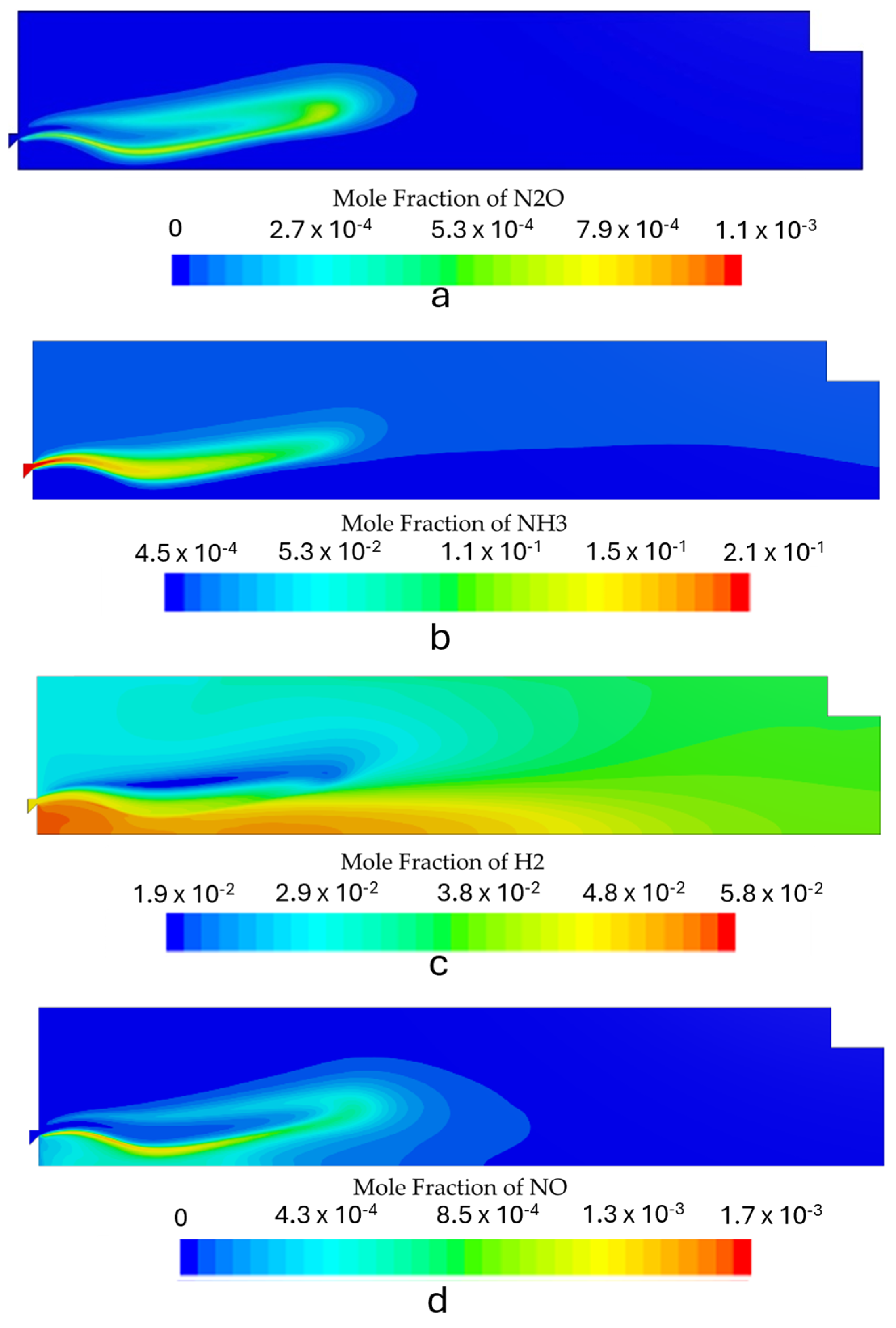
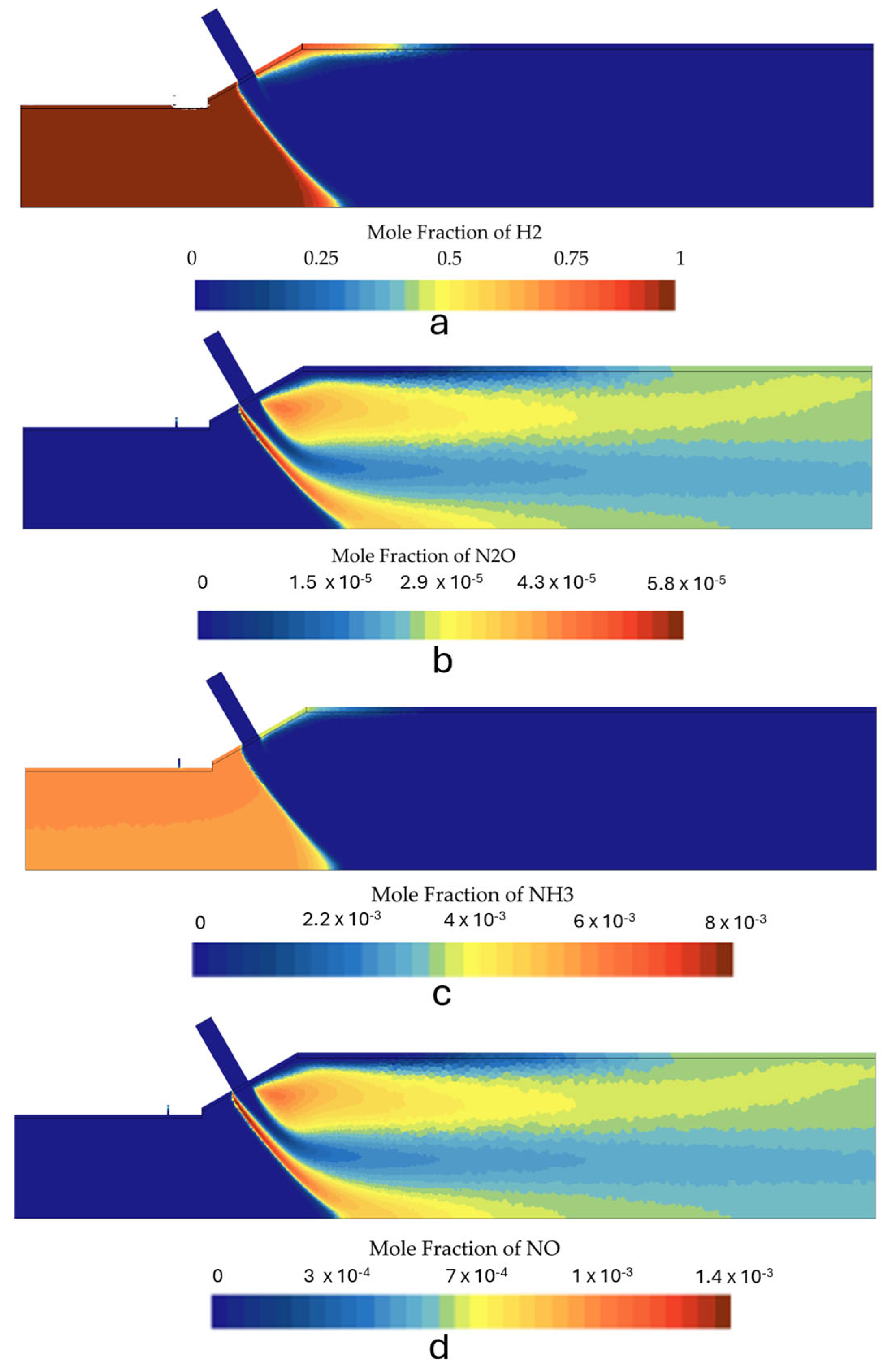
4.2. Species Concentration Contours

Figure 8, Figure 9 and Figure 10 show the contours of the most relevant species in ammonia combustion for each operating condition. The burner operation should minimize NO_x and N₂O emissions while maximizing the conversion process of NH₃ into H₂. The maximum mole concentration of H₂ occurs inside the recirculation zone for all the simulated power inputs, which is also the zone with the highest temperatures. The increase in the power output led to some differences in the species distribution inside the combustion chamber. The N₂O local molar concentration reached the highest value for the highest thermal input, which can be attributed to high reactant velocities and an incomplete combustion process, which reduces the H radical production and restricts N₂O consumption through the reaction of N₂O + H ⇌ N₂+ OH.

NO_x emissions also increased with rising thermal power. However, this trend was accompanied by a reduction in the NH₃ slip and an enhancement of the conversion process of NH₃ to H₂. The rise in NO_x emissions was marginal, with a maximum of 8 ppm, which remains well below the typical levels observed in standard combustion equipment. These findings are in agreement with the results of previous studies [6,15,45,46] that reported low NO_x emissions in the combustion of ammonia under fuel-rich conditions. The emissions from the first stage are presented in

Table 5. Species mole fractions (vol.% or ppm) for the first stage.

Species Concentration	4 kW	6 kW	8 kW
NOx ppm	1.3	4.7	7.8
H2%	4.7	4.8	4.9
NH3 ppm	8059	6989	6320
N2O ppm	~0	~0	~0

. Figure 11 shows the radial NO_x profile at the exit section, where the highest outlet temperatures correspond to higher NO_x emissions. This can be attributed to the combined effects of thermal and fuel NO_x generated through ammonia oxidation.

The maximum H₂ concentration is located in the IRZ, where the highest temperatures are present, which indicates that the temperature field highly controls the NH₃ oxidation process. The average H₂ molar fraction ranged from 4.7% to 4.9%. The predicted hydrogen concentration at the outlet of the first stage burner is consistent with results from previous experimental studies conducted under similar operating conditions using a comparable burner configuration, which served as the conceptual basis for the design of the current system. Experimental data reported a hydrogen mole fraction of approximately 4.4% [19], which closely aligns with the numerical predictions, showing only a minor deviation.

Regarding unburned ammonia, the predicted emissions for the simulated regimes demonstrated moderate accuracy, with the results presented in Table 5 falling within the range observed in experimental tests. In particular, the reference combustor yielded unburned ammonia concentrations of approximately 5000 ppm [19]. These results highlight the ability of the kinetic model to capture the sensitivity to NH₃ “cracking” and the dissociation phenomenon, which is a crucial parameter to model in an RQL application.

Flames with higher thermal inputs yield higher H₂ emissions. The radial temperature profile at the exit reveals that the highest temperatures correspond to the highest H₂ and the lowest NH₃ molar fractions, as shown in Figure 11. Additionally, higher NH₃ emissions occur near the wall for the lowest power output, while at higher thermal power, a more homogeneous NH₃ concentration profile is observed.

4.3. Second Stage Simulation

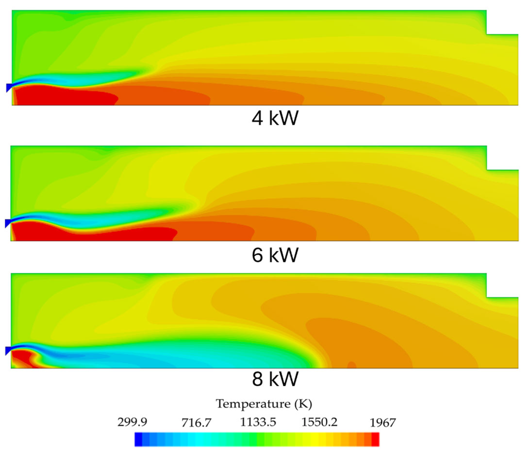
4.3.1. Cases 1 and 2: Effect of Thermal Input

A different approach was taken for the second stage of the combustor. For this simulation, different fuel injection strategies and geometries were investigated. Only the results for the base scenarios (cases 1 and 2 from Table 2) and the most promising operation regimes (cases 4 and 6 from Table 2) of the second stage are presented in detail. Simulations were performed for thermal powers ranging from 4 to 10 kW and for both configurations A and B (cases 1, 2, 4, and 6 in Table 2). The secondary fuel injection aims to maintain flame stability at the second stage while enhancing the mixture for complete combustion and reducing N₂O emissions and ammonia slip. The necessity and impact of this secondary fuel injection will be investigated in detail in an experimental measurements campaign on the geometry optimized in this numerical study.

Figure 12 shows the predicted temperature contours for various operating conditions. The NO_x, H₂, N₂O, and NH₃ species molar concentration contours for each case can be seen in Figure 13 and Figure 14.

Table 6. Emissions in vol.% and in ppm for the second stage simulations (see case conditions in Table 5).

Species	Case 1	Case 2	Case 3	Case 4	Case 5	Case 6	Case 7	Case 8
NOx ppm	680	504	599	581	687	491	478	556
H2 ppm	0	1	0	0	0	0	0	2
NH3 ppm	0.0	0.0	0	0	0	0	0	0
N2O ppm	7.73	2.5	30	9	6	1	38	13
H2O%	21.8	21.57	18.2	17.9	21.8	21.7	18.2	18.1
O2%	6.7	6.9	8.9	9.0	6.7	6.8	8.9	8.9
Temperature (K)	1306	1372	1086	1144	1263	1330	106	110

gives the composition of the combustion products at the outlet for all simulated conditions. The temperature contours reveal that the highest thermal power also yields the highest flame temperature. The peak temperature regions appeared downstream of the secondary air injection within its wake and in its upstream region where the cross-flow interacts with the secondary air jet. The increase in flame temperature at higher thermal inputs can be attributed to a faster and better mixing of air and reactants, leading to complete combustion and lower NO_x and N₂O emissions. These phenomena can be observed in detail in Figure 14, where case 2 presented lower NO_x and N₂O emissions compared to case 1 (Figure 13). It can also be observed that NH₃ is almost completely oxidized downstream of the secondary air jet, with both simulations predicting ammonia contents below 1 ppm. However, the combustion chamber still presents substantial NO_x emissions for current combustion applications, which led to the adoption of alternative strategies to mitigate these emissions.

4.3.2. Case 6: Effect of Secondary Air

The effect of secondary air is investigated by performing a simulation for configuration B. This configuration enables the combustor to operate with a higher inlet velocity for the secondary air injection. This increase was accomplished by means of a reduction of the inlet diameter from 8 mm to 6 mm, aiming to improve the mixing and, consequently, the combustion process. This modification led to a shorter high temperature region downstream of the secondary air injection and a higher penetration of the air jet towards the center of the combustion chamber. The higher penetration led to the formation of a recirculating region upstream of the air injection. This recirculation does not exist for simulations that use configuration A (cases 1, 2, 3, and 4). When operating at a power of 10 kW and a global equivalence ratio of Φ = 0.6 (cases 2 and 6), configuration B yielded lower NO_x values compared with configuration A, while keeping N₂O emissions to minimum levels. This effect can be observed in Figure 15, where the species contours are displayed, and we can observe that almost no N₂O is produced in case 6. In this case, NO_x formation occurs mainly inside the IRZ where temperatures are higher, and the thermal NO_x formation is the main mechanism. Dilution of the combustion products occurs due to the secondary air injection, decreasing the temperature and freezing the NO_x formation.

4.3.3. Case 4: Effect of Secondary Fuel

In case 4, the combustion chamber was fired without the addition of secondary fuel. This strategy was employed to increase the NH₃/H₂ ratio of the global fuel mixture and reduce the inherent complexity of additional fuel injection in real-life applications. Another important aspect is that the fuel mixture would ideally have a hydrogen ratio that could be obtained via local ammonia cracking instead of operating with two different fuel mixtures, which is one of the operational challenges of dual fuel technologies. The burner operated under the same configuration as case 2 but without the secondary fuel injection, lowering the power output from 10 to 8 kW and reducing the global equivalence ratio from 0.6 to approximately 0.5.

In this case, a peak temperature is located in the same location as observed in the case 1 and 2 simulations, occurring within the upstream shear layer of the jet similar to the previous mentioned simulations. The downstream peak temperature is lower than the upstream peak and the downstream flame is shorter compared to the case 2 simulation, as illustrated in Figure 12. The reduction in the peak temperature for case 4 can be attributed to the absence of the hydrogen injection that would enrich the mixture to be more reactive and achieve higher temperatures.

Figure 16 shows the species contours for this operating condition. The mixture burned completely and there was no NH₃ slip. However, both N₂O and NO_x emissions increased compared to case 2. Table 6 shows the emissions in vol.% and ppm for all the second stage burner simulations, which can be analyzed in detail and compared. Even though the N₂O emissions are only 9 ppm in case 4, it should be noted that this is a very critical issue since N₂O has a GWP 289 times greater than CO₂, and therefore its emissions should be kept to a minimum. However, it should be noted that simulations predicted a stable flame and that operating the burner without the secondary fuel injection is possible. H₂ played a significant role in reducing the N₂O emissions to minimum levels. The NO_x emissions also increased slightly compared to case 2 and case 6, with case 4 yielding the highest emissions among the simulations that used higher thermal input.

4.4. Exhaust Gas Emissions

In this section, the emissions from the combustion chamber are discussed in detail. The NH₃, NO_x, and N₂O emissions in the most promising conditions (cases 1, 2, 4, and 6) are given in

Table 7. Pollutant emissions in mg/Nm³ for the simulated conditions (dry basis, corrected to 15% O₂).

	NOx mg/Nm3	NH3 mg/Nm3	N2O mg/Nm3
Case 2	362	~ 0	2.6
Case 6	351	~ 0	1.5
Case 4	471	~ 0	10.5
Case 1	379	~ 0	6.3

in mg/NM³, according to the European Union directive 2010/75 [47]. These simulations were selected as the most promising operating conditions due to their balanced performance in terms of N₂O and NO_x emissions. They allowed for the lowest NO_x emissions among all conditions while maintaining minimal N₂O levels.

The values obtained for the NO_x emissions presented similar ranges with previous works in the literature, where the NO_x emissions for staged combustion chamber operation with ammonia yielded similar NO_x emissions for a global equivalence ratio of 0.6 with approximately 330 mg/NM³ [48]. This highlights the capacity to predict the pollutant emissions at different equivalence ratios, at both the first and second stages.

Regarding N₂O, the predicted emissions yielded relatively low levels, which are also in line with other combustion works. Although not directly comparable with the current design, a swirl burner operating under a lean regime with an equivalence ratio of 0.65 yielded less than 20 ppm of N₂O for the highest power output [49]. Another numerical and experimental study investigated the combustion of cracked and partially cracked ammonia at an equivalence ratio of 0.9. Although the operating conditions were not directly comparable to the current work, the study also reported low N₂O emissions, with experimental results showing less than 10 ppm for both pure and cracked ammonia [50].

It can be concluded that case 6 is the most promising operating regime as it yields the lowest NO_x and N₂O emissions. Although cases 1 and 2 presented higher emissions for both N₂O and NO_x, their absolute differences were relatively small, with the highest deviations being 28 mg/Nm³ for NO_x and 5 mg/Nm³ for N₂O in case 1 (Table 7).

Other operating conditions should also be addressed, such as case 7 (Table 6), which presented the lowest NO_x emissions among all the simulated cases. However, this condition also presented the highest N₂O emissions. Based on the emissions presented in Table 7, it can be concluded that none of the simulated conditions achieved NO_x emission levels within the legislation limits [47]. Therefore, De-NO_x treatment solutions are necessary, as the emissions do not comply with local directives. Technologies such as post-combustion SCR treatment are currently under development for marine combustion engines. MAN Energy Solutions already announced the first iteration of an SCR catalytic converter for a marine ammonia engine that passed factory tests [51]. The unit is an adaptation from existing SCR technology, originally developed for cruise and cargo ships to reduce NO_x emissions from conventional marine engines. Nikki-universal has also been developing catalyst technologies for De-NO_x, De-N₂O, and De-NH₃ for combustion application [52], which would be fundamental to the fast implementation of ammonia combustion technologies while keeping emissions under legislation limits.

4.5. Greenhouse Gas Emissions

This section assesses the impact of ammonia combustion on global warming. Since ammonia does not emit CO₂ during combustion, it is a promising fuel for applications like gas turbines, boilers, and internal combustion engines, allowing for the retrofitting of existing infrastructure without full replacement, accelerating the transition to sustainable fuels.

Global warming potential (GWP) is commonly used to evaluate environmental impact. GWP is defined as the time-integrated radiative forcing from the pulsed emission of a gas, expressed either in absolute terms (AGWP) or relative to CO₂ (GWP) [53,54]. It is typically evaluated over 20- and 100-year timeframes [55]. Although N₂O is a potent GHG with a GWP₁₀₀ of 298, the GWP of NO_x is variable and highly dependent on emission location and altitude. Estimates range from GWP₂₀ = 30–33 to GWP₁₀₀ = 7–10 for surface emissions [53] and up to 59 for high-altitude sources [56].

The literature considers the impact of NH₃ in the GWP as non GHG emissions. However, due to its toxicity, it is a pollutant with a high local impact, and its emissions should be kept to a minimum. The values of GWP for 20- and 100-year timeframes are summarized in

Table 8. Global warming potential (GWP) for NH₃, NO_x, and N₂O (compared with CO₂) for the 20-year and 100-year timeframes.

	NOx	NH3	N2O	CO2
GWP20 years	33 *	~0	273	1
GWP100 years	10 *	~0	298	1

* worst case scenario for ground emissions [55].

.

Table 9. CO₂-equivalent Emissions of Greenhouse Gases Based on GWP Factors.

	NOx mg/kWh	NH3 mg/kWh	N2O mg/kWh	g CO2eq 20 years /kWh	g CO2eq 100 years/kWh
Case 2	100.3	0.0	0.7	4.9	1.2
Case 6	99.0	0.0	0.4	4.8	1.1
Case 4	143.7	0.0	3.2	7.7	2.3
Case 1	137.8	0.0	2.3	7.1	2.0

shows the CO₂-equivalent emissions for combustor operation. The CO₂-equivalent emissions are small compared to conventional combustion operations, with the highest emissions (about 8 g/kWh CO₂ equivalents) occurring in case 4. This magnitude of emissions is far lower than the average combined-cycle gas turbine, which presents an average value of approximately 429 g CO₂ equivalents/kWh.

Table 10. CO₂ emissions per kWh for various power generation technologies.

Energy Source	CO2 Emissions (gCO2/kWh)	Reference
Coal	~986	RTE FRANCE [57]
Oil-based Generation	~777	RTE FRANCE [57]
Natural Gas (combined cycle)	~429	RTE FRANCE [57]
Biomass	~230	IPCC [58]
Nuclear	~12	IPCC [58]
Hydropower	~24	IPCC [58]
Wind Power	~11	IPCC [58]
Solar PV	~41	IPCC [58]

shows the equivalent CO₂ emissions for the most common energy production sources. The table facilitates a comparative analysis of CO₂-equivalent emissions from conventional energy sources and those obtained under the combustion chamber conditions detailed in Table 9. It should be noted that only the emissions from the combustion chamber operation were accounted for in this analysis. The CO₂-equivalent emissions from NH₃ or H₂ production, storage, and transportation were not considered. Moreover, the values obtained in this study highlight the possibility of reducing the greenhouse effect impact in combustion applications by using ammonia as a direct fuel or through co-firing it with conventional fuels.

4.6. Pratical Implications

In this section, the combustion chamber is evaluated in terms of performance for different design parameters, such as the pollutant emissions that have a local impact and greenhouse gas emissions that have a global impact. Geometry B presented the best emissions performance in case 6 when operating with the secondary fuel injection, highlighting the impact of H₂ as a combustion promoter and an inhibitor in N₂O formation. However, geometry A in case 4 also presented a promising performance to apply the RQL strategy for ammonia combustion without secondary fuel injection. Although its CO₂ equivalence is higher when compared to the secondary fuel counterpart (case 6), its value is still 30 times lower than the average combined-cycle gas turbine, highlighting that there is still room to explore and improve a design that maximizes the NH₃ content in the fuel mixture. This would improve the easiness of implementation in real-life applications where, ideally, the burner would operate on pure ammonia or in an NH₃/H₂ mixture that would be possibly obtainable through cracking of NH₃ into an H₂/NH₃/N₂ mixture. The necessity of dual fuel operation might be a logistical and operational challenge for industrial applications. Several research groups have already tackled this hypothesis [59,60,61] where ammonia would be dissociated with the heat recovered from the combustion chamber.

5. Conclusions

The CFD simulation of an RQL combustion chamber fired by mixtures of NH₃/H₂ was performed in this work. The results showed that the first stage was able to operate stably under fuel-rich conditions while keeping NO_x and N₂O at minimum levels. During the first stage of operation, NH₃ emissions are expected to exceed the acceptable ammonia concentration in the flue gas due to the incomplete conversion into hydrogen. Although the conversion efficiency was not 100%, a significant portion of the surplus ammonia was successfully transformed into H₂, with the highest observed molar fraction reaching 4.9% and an ammonia concentration of 6320 ppm. The results align with previous experimental and numerical work findings [19], highlighting the potential of the CFD RANS simulation to develop preliminary combustion chamber designs without the necessity of more complex turbulent modeling. This work demonstrates the potential of moderately demanding CFD simulation for R&D applications, where a simplified turbulence RANS model coupled with a detailed chemistry model can be a powerful tool to investigate different geometries and firing strategies while preserving core fundamental physics. However, it should be noted that this methodology presents certain limitations due to the absence of direct experimental validation for the second stage combustion chamber. Moreover, this approach can offer valuable insights for geometry development and optimization, the prediction of flame location, and dimensional design.

Future work will focus on conducting detailed experimental campaigns to validate the numerical findings. More specifically, exhaust gas measurements will be performed to verify emission predictions and unburned ammonia slip. At the same time, axial temperature profiles will provide deeper insights into the thermal distribution within the combustion chamber. Chemiluminescence measurements are also planned to improve our understanding of reaction mechanisms and flame dynamics. Additionally, combustion stability tests will be carried out to validate the envisaged combustion regimes and assess the combustion chamber’s operational envelope. These experimental results will refine the model and aid in developing a more optimized combustion chamber design.

Regarding the second stage, different firing strategies and geometries were simulated using the same numerical methodologies as the first stage. All simulated flames predicted complete NH₃ oxidation, with the major differences being in the predicted NO_x and N₂O emissions. The main conclusions drawn from the analysis can be summarized as follows:

• The emissions from the RQL combustor show the potential to fire mixtures of H₂/NH₃ to produce power while keeping CO₂-equivalent emissions to minimum levels. Case 6 yielded a GWP CO_2equivalent/kWh of only 1.1, highlighting the potential of ammonia combustion to reduce greenhouse gas emissions in combustion applications.
• The second stage NO_x emissions exceeded the legislation levels (250 mg/Nm³) for all the simulations. This shows the necessity of catalytic treatment to keep emissions at acceptable levels. Case 6 predicted a concentration of 350 mg/Nm³ of NO_x, which is not yet able to comply with legislation despite being the lowest NO_x emissions among the simulated operating conditions.
• The addition of H₂ as a secondary fuel (cases 1, 2, 5, and 6) enabled the reduction of N₂O emissions to single digit values. The second stage of the combustion chamber was able to operate without the necessity of a secondary fuel, although at the expense of an increase in N₂O emissions. This configuration resulted in the lowest NO_x emissions among all scenarios. However, it also exhibited the highest predicted N₂O emissions, indicating a trade-off between NO_x mitigation and N₂O formation. This trade-off highlights the challenge of simultaneously minimizing both pollutants in ammonia combustion.
• A pathway should be focused on using fuel mixtures with higher NH₃ contents and, preferably, design a combustion chamber that can operate with pure ammonia to minimize the logistic constraints of dual fuel operation. A possible solution for the inability to stably burn and minimize ammonia slip is to perform a local dissociation of ammonia into H₂/NH₃ mixtures to enhance the fuel combustion properties.

References

- United Nations. Paris Agreement. In United Nations Framework Convention on Climate Change; United Nations: Paris, France, 2015. [Google Scholar]
- Saygin, D.; Blanco, H.; Boshell, F.; Cordonnier, J.; Rouwenhorst, K.; Lathwal, P.; Gielen, D. Ammonia Production from Clean Hydrogen and the Implications for Global Natural Gas Demand. Sustainability 2023, 15, 1623. [Google Scholar] [CrossRef]
- Wang, B.; Li, T.; Gong, F.; Othman, M.H.D.; Xiao, R. Ammonia as a Green Energy Carrier: Electrochemical Synthesis and Direct Ammonia Fuel Cell—A Comprehensive Review. Fuel Process. Technol. 2022, 235, 107380. [Google Scholar] [CrossRef]
- IEA. Ammonia Technology Roadmap Towards More Sustainable Nitrogen Fertiliser Production; IEA: Paris, France, 2021. [Google Scholar]
- Cardoso, J.P. Ammonia as a Decarbonization Tool for Low Carbon Fuel Applications and Stationary Power Generation. Ph.D. Thesis, Instituto Superior Técnico, Lisbon, Portugal, 2024. [Google Scholar]
- Kobayashi, H.; Hayakawa, A.; Somarathne, K.D.K.A.; Okafor, E.C. Science and Technology of Ammonia Combustion. Proc. Combust. Inst. 2019, 37, 109–133. [Google Scholar] [CrossRef]
- Alnajideen, M.; Shi, H.; Northrop, W.; Emberson, D.; Kane, S.; Czyzewski, P.; Alnaeli, M.; Mashruk, S.; Rouwenhorst, K.; Yu, C.; et al. Ammonia Combustion and Emissions in Practical Applications: A Review. Carbon Neutrality 2024, 3, 13. [Google Scholar] [CrossRef]
- Pacheco, G.; Pereira, J.; Mendes, M.; Coelho, P. Investigation of a Fuel-Flexible Diffusion Swirl Burner Fired with NH3 and Natural Gas Mixtures. Energies 2024, 17, 4206. [Google Scholar] [CrossRef]
- Mission Possible Partnership. Making Net-Zero Ammonia Possible. 2022. Available online: https://www.energy-transitions.org/publications/making-net-zero-ammonia-possible/ (accessed on 12 February 2025).
- Mission possible Partnership. MPP Global Project Tracker. January 2025. Available online: https://tracker.missionpossiblepartnership.org/mpp-global-projects-map/ (accessed on 19 January 2025).
- Afif, A.; Radenahmad, N.; Cheok, Q.; Shams, S.; Kim, J.H.; Azad, A.K. Ammonia-Fed Fuel Cells: A Comprehensive Review. Renew. Sustain. Energy Rev. 2016, 60, 822–835. [Google Scholar] [CrossRef]
- Zhou, F.; Yu, J.; Wu, C.; Fu, J.; Liu, J.; Duan, X. The Application Prospect and Challenge of the Alternative Methanol Fuel in the Internal Combustion Engine. Sci. Total Environ. 2024, 913, 169708. [Google Scholar] [CrossRef]
- Lan, R.; Tao, S. Ammonia as a Suitable Fuel for Fuel Cells. Front. Energy Res. 2014, 2, 35. [Google Scholar] [CrossRef]
- Giuntini, L.; Frascino, L.; Ariemma, G.B.; Sorrentino, G.; Galletti, C.; Ragucci, R. Modeling of Ammonia MILD Combustion in Systems with Internal Recirculation. Combust. Sci. Technol. 2023, 195, 3513–3528. [Google Scholar] [CrossRef]
- Rocha, R.C.; Costa, M.; Bai, X.S. Combustion and Emission Characteristics of Ammonia under Conditions Relevant to Modern Gas Turbines. Combust. Sci. Technol. 2021, 193, 2514–2533. [Google Scholar] [CrossRef]
- Okafor, E.C.; Naito, Y.; Colson, S.; Ichikawa, A.; Kudo, T.; Hayakawa, A.; Kobayashi, H. Experimental and Numerical Study of the Laminar Burning Velocity of CH4–NH3–Air Premixed Flames. Combust Flame 2018, 187, 185–198. [Google Scholar] [CrossRef]
- Kurata, O.; Iki, N.; Matsunuma, T.; Inoue, T.; Tsujimura, T.; Furutani, H.; Kobayashi, H.; Hayakawa, A. Performances and Emission Characteristics of NH3-Air and NH3-CH4-Air Combustion Gas-Turbine Power Generations. Proc. Combust. Inst. 2017, 36, 3351–3359. [Google Scholar] [CrossRef]
- Romano, C.; Cerutti, M.; Babazzi, G.; Miris, L.; Lamioni, R.; Galletti, C.; Mazzotta, L.; Borello, D. Ammonia Blends for Gas-Turbines: Preliminary Test and CFD-CRN Modelling. Proc. Combust. Inst. 2024, 40, 105494. [Google Scholar] [CrossRef]
- Pacheco, G.P.; Rocha, R.C.; Franco, M.C.; Mendes, M.A.A.; Fernandes, E.C.; Coelho, P.J.; Bai, X.S. Experimental and Kinetic Investigation of Stoichiometric to Rich NH3/H2/Air Flames in a Swirl and Bluff-Body Stabilized Burner. Energy Fuels 2021, 35, 7201–7216. [Google Scholar] [CrossRef]
- Li, R.; Konnov, A.A.; He, G.; Qin, F.; Zhang, D. Chemical Mechanism Development and Reduction for Combustion of NH3/H2/CH4 Mixtures. Fuel 2019, 257, 116059. [Google Scholar] [CrossRef]
- Stagni, A.; Arunthanayothin, S.; Dehue, M.; Herbinet, O.; Battin-Leclerc, F.; Bréquigny, P.; Mounaïm-Rousselle, C.; Faravelli, T. Low- and Intermediate-Temperature Ammonia/Hydrogen Oxidation in a Flow Reactor: Experiments and a Wide-Range Kinetic Modeling. Chem. Eng. J. 2023, 471, 144577. [Google Scholar] [CrossRef]
- Okafor, E.C.; Naito, Y.; Colson, S.; Ichikawa, A.; Kudo, T.; Hayakawa, A.; Kobayashi, H. Measurement and Modelling of the Laminar Burning Velocity of Methane-Ammonia-Air Flames at High Pressures Using a Reduced Reaction Mechanism. Combust Flame 2019, 204, 162–175. [Google Scholar] [CrossRef]
- Ren, J.; Li, W.; Zou, C. Development of a Reduced Combustion Model for Ammonia/Hydrogen Combustion. Fuel 2023, 354, 129389. [Google Scholar] [CrossRef]
- Fatehi, M.; Renzi, M. Modelling and Development of Ammonia-Air Non-Premixed Low NOX Combustor in a Micro Gas Turbine: A CFD Analysis. Int. J. Hydrogen Energy 2024, 88, 1–10. [Google Scholar] [CrossRef]
- Mazzotta, L.; Lamioni, R.; D’Alessio, F.; Meloni, R.; Morris, S.; Goktepe, B.; Cerutti, M.; Romano, C.; Creta, F.; Galletti, C.; et al. Modeling Ammonia-Hydrogen-Air Combustion and Emission Characteristics of a Generic Swirl Burner. J. Eng. Gas Turbine Power 2024, 146, 091022. [Google Scholar] [CrossRef]
- Xiao, H.; Valera-Medina, A.; Bowen, P.J. Modeling Combustion of Ammonia/Hydrogen Fuel Blends under Gas Turbine Conditions. Energy Fuels 2017, 31, 8631–8642. [Google Scholar] [CrossRef]
- Okafor, E.C.; Kurata, O.; Yamashita, H.; Iki, N.; Inoue, T.; Jo, H.; Shimura, M.; Tsujimura, T.; Hayakawa, A.; Kobayashi, H. Achieving High Flame Stability with Low NO And Zero N2O and NH3 Emissions during Liquid Ammonia Spray Combustion with Gas Turbine Combustors. Proc. Combust. Inst. 2024, 40, 105340. [Google Scholar] [CrossRef]
- Shih, T.-H.; Liou, W.W.; Shabbir, A.; Yang, Z.; Zhu, J. A new K-epsilon eddy viscosity model for high reynolds numer turbulent flows. Comput. Fluids 1995, 24, 227–238. [Google Scholar] [CrossRef]
- Spalart, P.R.; Rumsey, C.L. Effective Inflow Conditions for Turbulence Models in Aerodynamic Calculation. AIAA J. 2007, 45, 10. [Google Scholar] [CrossRef]
- Baulch, D.L.; Bowman, C.T.; Cobos, C.J.; Cox, R.A.; Just, T.; Kerr, J.A.; Pilling, M.J.; Stocker, D.; Troe, J.; Tsang, W.; et al. Evaluated Kinetic Data for Combustion Modeling: Supplement II. J. Phys. Chem. Ref. Data 2005, 34, 757–1397. [Google Scholar] [CrossRef]
- Siemens Industries Digital Software Realizable K-Epsilon Model. In SIEMENS STAR-CCM+ Documentation; Siemens: Munich, Germany, 2020.
- Li, Y.; Sarathy, S.M. Probing hydrogen–nitrogen chemistry: A theoretical study of important reactions in NxHy, HCN and HNCO oxidation. Int. J. Hydrogen Energy 2020, 45, 23624–23637. [Google Scholar] [CrossRef]
- Klippenstein, S.J.; Harding, L.B.; Ruscic, B.; Sivaramakrishnan, R.; Srinivasan, N.K.; Su, M.C.; Michael, J.V. Thermal Decomposition of NH2OH and Subsequent Reactions: Ab Initiotransition State Theory and Reflected Shock Tube Experiments. J. Phys. Chem. A 2009, 113, 10241–10259. [Google Scholar] [CrossRef]
- Abian, M.; Alzueta, M.U.; Glarborg, P. Formation of NO from N2/O2 Mixtures in a Flow Reactor: Toward an Accurate Prediction of Thermal NO. Internatonal J. Chem. Kinet. 2015, 47, 518–532. [Google Scholar] [CrossRef]
- Veynante, D.; Vervisch, L. Turbulent Combustion Modeling. Prog. Energy Combust. Sci. 2002, 28, 193–266. [Google Scholar] [CrossRef]
- Siemens Industries Digital Software. Reacting Species Transport. In SIEMENS STAR-CCM+ Documentation; Siemens: Munich, Germany, 2020. [Google Scholar]
- Klimanek, A.; Adamczyk, W.; Sładek, S.; Fan, Y.; Bothien, M.R.; Gruber, A.; Szlęk, A. Prediction of Ammonia Ignition/Quenching and Emissions of NOx, NH3 and H2 in a Non-Premixed Swirl Combustor Using the EDC Model. Case Stud. Therm. Eng. 2025, 65, 105670. [Google Scholar] [CrossRef]
- Kuang, Y.; Han, D.; Xu, Z.; Wang, Y.; Wang, C. Numerical Study on Combustion Characteristics of Ammonia Mixture under Different Combustion Modes. Int. J. Hydrogen Energy 2024, 54, 1403–1409. [Google Scholar] [CrossRef]
- Siemens Industries Digital Software Participating Media Radiation (DOM). In SIEMENS STAR-CCM+ Documentation; Siemens: Munich, Germany, 2020.
- Modest, M.F. Narrow-Band and Full-Spectrum k-Distributions for Radiative Heat Transfer-Correlated-k vs. Scaling Approximation. J. Quant. Spectrosc. Radiat. Transf. 2003, 76, 69–83. [Google Scholar] [CrossRef]
- Mazumder, S.; Roy, S.P. Modeling Thermal Radiation in Combustion Environments: Progress and Challenges. Energies 2023, 16, 4250. [Google Scholar] [CrossRef]
- Liu, Y.; Zhu, J.; Liu, G.; Liu, F.; Consalvi, J.-L. Assessment of Various Full-Spectrum Correlated K-Distribution Methods in Radiative Heat Transfer in Oxy-Fuel Sooting Flames. Int. J. Therm. Sci. 2023, 184, 107919. [Google Scholar] [CrossRef]
- Wang, C.; Modest, M.F.; Ren, T.; Cai, J.; He, B. Comparison and Refinement of the Various Full-Spectrum k-Distribution and Spectral Line Weighted-Sum-of-Gray-Gases Models for Nonhomogeneous Media. J. Quant. Spectrosc. Radiat. Transf. 2021, 271, 107695. [Google Scholar] [CrossRef]
- Zhou, Y.; Wang, C.; Ren, T.; Zhao, C. A Machine Learning Based Full-Spectrum Correlated k-Distribution Model for Nonhomogeneous Gas-Soot Mixtures. J. Quant. Spectrosc. Radiat. Transf. 2021, 268, 107628. [Google Scholar] [CrossRef]
- Khateeb, A.A.; Guiberti, T.F.; Zhu, X.; Younes, M.; Jamal, A.; Roberts, W.L. Stability Limits and NO Emissions of Technically-Premixed Ammonia-Hydrogen-Nitrogen-Air Swirl Flames. Int. J. Hydrogen Energy 2020, 45, 22008–22018. [Google Scholar] [CrossRef]
- Mashruk, S.; Shi, H.; Mazzotta, L.; Ustun, C.E.; Aravind, B.; Meloni, R.; Alnasif, A.; Boulet, E.; Jankowski, R.; Yu, C.; et al. Perspectives on NOX Emissions and Impacts from Ammonia Combustion Processes. Energy Fuels 2024, 18, 19253–19292. [Google Scholar] [CrossRef]
- Official Journal of the European Union. DIRECTIVE 2010/75/EU; European Union: Brussels, Belgium, 2010. [Google Scholar]
- Okafor, E.C.; Somarathne, K.D.K.A.; Hayakawa, A.; Kudo, T.; Kurata, O.; Iki, N.; Kobayashi, H. Towards the Development of an Efficient Low-NOx Ammonia Combustor for a Micro Gas Turbine. Proc. Combust. Inst. 2019, 37, 4597–4606. [Google Scholar] [CrossRef]
- Mashruk, S.; Okafor, E.C.; Kovaleva, M.; Alnasif, A.; Pugh, D.; Hayakawa, A.; Valera-Medina, A. Evolution of N2O Production at Lean Combustion Condition in NH3/H2/Air Premixed Swirling Flames. Combust Flame 2022, 244, 112299. [Google Scholar] [CrossRef]
- An, Z.; Zhang, W.; Zhang, M.; Xing, J.; Kai, R.; Lin, W.; Wang, R.; Wang, J.; Huang, Z.; Kurose, R. Experimental and Numerical Investigation on Combustion Characteristics of Cracked Ammonia Flames. Energy Fuels 2024, 38, 7412–7430. [Google Scholar] [CrossRef]
- Ammonia Energy Association. Selective Catalytic Reduction for Marine Ammonia Engines. January 2024. Available online: https://ammoniaenergy.org/articles/selective-catalytic-reduction-for-marine-ammonia-engines/ (accessed on 12 February 2025).
- suji, I.; Ikoma, T.; Okamoto, H.; Aoi, N. Exhaust Gas Treatment Catalysts for Ammonia-Fueled Engines. Ammonia Energy Conference. 2022. Available online: https://ammoniaenergy.org/presentations/exhaust-gas-treatment-catalysts-for-ammonia-fueled-engines/ (accessed on 12 February 2025).
- Lasek, J.A.; Lajnert, R. On the Issues of NOx as Greenhouse Gases: An Ongoing Discussion…. Appl. Sci. 2022, 12, 10429. [Google Scholar] [CrossRef]
- Fuglestvedt, J.S.; Shine, K.P.; Berntsen, T.; Cook, J.; Lee, D.S.; Stenke, A.; Skeie, R.B.; Velders, G.J.M.; Waitz, I.A. Transport Impacts on Atmosphere and Climate: Metrics. Atmos. Environ. 2010, 44, 4648–4677. [Google Scholar] [CrossRef]
- Lammel, G.; Graßl, H. Greenhouse Effect of NOx Review Articles. Environ. Sci. Pollut. Res. 1995, 2, 40–45. [Google Scholar] [CrossRef]
- Skowron, A.; Lee, D.S.; De León, R.R. Variation of Radiative Forcings and Global Warming Potentials from Regional Aviation NOx Emissions. Atmos. Environ. 2015, 104, 69–78. [Google Scholar] [CrossRef]
- RTE France. Réseau de Transport d’Électricité ECO2mix—CO2 Emissions per KWh of Electricity Generated in France. January 2025. Available online: https://www.rte-france.com/en/eco2mix/co2-emissions (accessed on 12 February 2025).
- Schlömer, S.; Bruckner, T.; Fulton, L.; Hertwich Austria, E.; McKinnon, A.U.; Perczyk, D.; Roy, J.; Schaeffer, R.; Hänsel, G.; de Jager, D.; et al. Annex III: Technology-specific cost and performance parameters. In Climate Change 2014: Mitigation of Climate Change. Contribution of Working Group III to the Fifth Assessment Report of the Intergovernmental Panel on Climate Change; Cambridge University Press: Cambridge, UK; New York, NY, USA, 2014. [Google Scholar]
- Kim, N.; Lee, M.; Park, J.; Park, J.; Lee, T. A Comparative Study of NOx Emission Characteristics in a Fuel Staging and Air Staging Combustor Fueled with Partially Cracked Ammonia. Energies 2022, 15, 9617. [Google Scholar] [CrossRef]
- Mei, B.; Zhang, J.; Shi, X.; Xi, Z.; Li, Y. Enhancement of Ammonia Combustion with Partial Fuel Cracking Strategy: Laminar Flame Propagation and Kinetic Modeling Investigation of NH3/H2/N2/Air Mixtures up to 10 Atm. Combust Flame 2021, 231, 111472. [Google Scholar] [CrossRef]
- Romano, C.; Bellotti, D.; Pucci, E.; Fadlun, E.; Roma, M.; Ghezzi, S.; Manferino, G.; Anfosso, C.; Monacchini, C. Ammonia Cracking As Auxiliary System for Gas Turbine: Preliminary Studies. In Proceedings of the ASME 2024 Power Conference, Washington, DC, USA, 15–18 September 2024. [Google Scholar] [CrossRef]