Improved Discrete-Time Active Disturbance Rejection Control for Enhancing Dynamics of Current Loop in LC-Filtered SPMSM Drive System

Abstract

Active disturbance rejection control is implemented in a LC-filtered surface-mounted permanent magnet synchronous motor (SPMSM) drive system to enhance current control dynamics. However, the combined effects of computation one-beat delay and the pulse-width modulation zero-order hold (ZOH) effect significantly degrade system stability and dynamic performance. To address these limitations, an improved predictive extended state observer (ESO) with an accurate ZOH discretization method is proposed to ensure fast and robust dynamic performance. The predictive ESO predicts one beat to compensate for the delay effect, while the ZOH discretization yields a more precise discrete dynamic model of the system. These combined improvements substantially enhance the system’s phase and gain margins, leading to superior dynamic performance. Furthermore, a discrete-domain transfer function of the control system is analytically derived, with the control parameters systematically designed using frequency-domain analysis to guarantee robust performance. Experimental validation on a LC-filtered SPMSM drive system demonstrates remarkable enhancement in current control dynamics while maintaining sufficient robustness.

1. Introduction

In pursuit of reliable operation and high torque density, a surface-mounted permanent magnet synchronous motor (SPMSM) is frequently applied to a system with voltage-source inverter (VSI) connected [1]. For applications such as long-cable fed drive [2], wide-bandgap semiconductor-based VSI [3] and high-speed motor systems [4], an LC filter is needed to suppress the negative effects of high dv/dt in PWM waveform on the stator insulation of SPMSM. The integration of an LC filter in the system may introduce resonance issues, significantly degrading the dynamic performance of motor current control, thereby limiting its applicability in high-performance applications [5]. Therefore, developing a control strategy with enhanced dynamic response becomes crucial.

Extensive research efforts have been devoted to developing advanced control strategies for LC-filtered SPMSM current regulation, as evidenced in [6,7,8,9,10,11,12,13,14,15,16,17]. These approaches encompass model predictive control (MPC) [6,7,8], active damping techniques (AD) [9,10,11], and triple-cascaded proportional-integral control (TCPI) [12,13]. These methodologies demonstrate substantial improvements in resonance attenuation and dynamic response compared to conventional PI controllers [14]. However, they are intrinsically limited by the fundamental constraints of digital control systems. Specifically, the inevitable one-beat computational delay and zero-order hold (ZOH) effects pose significant challenges. These inherent limitations present significant challenges in achieving further enhancements in transient response performance.

Digital control, with its high programmability and widespread industrial use, is limited by one-beat delay and ZOH effects. In traditional continuous-domain controller design, the one-beat delay and ZOH effect can be approximated as a delay of one and a half sampling periods [15,16]. In motor control, this delay is represented as a lagging angle in the rotating dq-axis, providing an equivalent spatial interpretation of digital computation delay [17]. Such delays can generate output voltages with phase retardation in both d-axis and q-axis, resulting in reduced stability margins and degraded dynamic performance [18].

To deal with the one-beat delay and ZOH effect in SPMSM control without LC filter, there are strategies, including the phase-lead corrector [19,20], deadbeat prediction [21,22], and discrete-domain pole-zero assignment [23,24]. The phase-lead correction method proposed in [19] is popularly used in motor control applications. In this method, the time-delay effect is compensated by introducing a phase-lead correction prior to the inverse Park transformation. This correction is achieved by calculating the hysteretic rotation angle through the product of the measured angular velocity and one and a half sampling periods [20]. While effective, this phase-lead correction method exhibits limited dynamic performance [25] and may lead to system instability under high-speed operating conditions [26]. Deadbeat prediction has emerged as a prevalent delay compensation technique in digital control systems. This method employs system model-based one-beat prediction to counteract the computational delay inherent in digital processors, thereby significantly enhancing transient response characteristics [21,22]. Nevertheless, its performance is critically dependent on precise parameter matching. Practical implementations reveal that parameter deviations can induce oscillatory instability and steady-state tracking errors, severely degrading system robustness. In comparison, discrete-domain pole-zero assignment demonstrates superior parameter robustness through explicit specification of closed-loop pole locations [23]. By incorporating the time delay as an inherent component of the discrete system model, this approach achieves effective delay compensation while maintaining stability margins [24]. However, the absence of predictive compensation necessitates conservative phase margin allocation. Therefore, the advantages of deadbeat prediction and discrete-domain pole-zero assignment can be combined to generate one-beat prediction while ensuring system robustness through pole placement.

Active disturbance rejection control (ADRC), a derivative of the classic PID controller, retains the strong practical applicability and ease of parameter tuning characteristic of PID controllers. By employing a tracking differentiator (TD), extended state observer (ESO), and state error feedback (SEF), ADRC significantly improves both the dynamic response and robustness of the system [27,28]. An observer-based control method has been extensively applied in SPMSM drive systems, including address parameter uncertainties [29], current control [30], speed regulation [31], and sensorless control strategies [32]. In the field of LC-filtered SPMSM control, current control systems face heightened susceptibility to multiple disturbance sources. These include pronounced resonance phenomena induced by LC filter dynamics and cross-coupling effects between dq-axes, which can collectively drive the system towards instability if not properly compensated. Owing to its superior disturbance rejection capabilities, ADRC has witnessed expanding industrial adoption, particularly in applications requiring robust resonance attenuation and rapid dynamic compensation [33,34,35,36]. The application of ADRC has been further extended to LCL-type grid-connected inverters, where it effectively mitigates resonance phenomena and reduces current harmonics. Building on these developments, a third-order ADRC architecture was proposed in [34], which introduces the estimated first derivative of current as an additional damping term for resonance suppression. Alternative approaches include the first-order system approximation method in [35], which leverages capacitor current feedback to provide inherent damping characteristics. The resonant ESO technique in [36] estimates resonance information for adaptive controller design. However, despite these significant contributions, existing methodologies have not adequately addressed the critical challenges posed by computational delays and discretization effects in digital control systems.

Various improved discretization methods have been proposed for its practical implementation. In the transition from continuous to discrete domain, a current-observer-based observer structure was developed in [37], while [38] employed the Euler method to derive the discrete observer matrix. Predictive schemes have been effectively incorporated into ADRC to mitigate delay effects [39,40]. The study in [39] cascades a Smith predictor with the ADRC observer, demonstrating superior uncertainty tolerance and delay compensation compared to conventional prediction methods. Furthermore, Ref. [40] introduces a predictive ADRC design utilizing fixed-time prediction instead of the Smith predictor, achieving enhanced robustness and faster dynamic response. However, these ADRC discretization approaches fail to specifically address the one-beat computation delay, and the ZOH effect remains unmitigated. Consequently, the dynamic performance of ADRC-based current control in LC-filtered SPMSM systems cannot be guaranteed.

Although Euler discretization and current observers offer structural simplicity and implementation ease, their direct applications in LC-filtered SPMSM current control demonstrate limited performance. This limitation stems from two fundamental issues: Euler discretization inadequately represents the discrete dynamics of PWM voltage inputs, while current observers fail to compensate for the inherent one-step computation delay in digital control. These deficiencies amplify resonance issues in LC-filtered SPMSM systems, significantly degrading both phase and gain margins. Consequently, the dynamic performance of ADRC-based current control is substantially compromised, restricting the application of LC-filtered SPMSM in high-performance drive systems requiring fast dynamic response.

To address these limitations, this paper proposes an enhanced ADRC discretization method. The proposed method improves the current control loop by incorporating ZOH discretization instead of Euler discretization and introducing an improved predictive observer to replace the conventional current observer, significantly enhancing both dynamic performance and system stability. The main contributions of this work are threefold:

(1)

A comprehensive comparison demonstrating the superior performance of ZOH discretization in accurately modeling discrete system dynamics and the enhanced delay compensation capability of the proposed predictive observer over conventional approaches, establishing the necessity of the proposed method for high-performance applications.

(2)

Development of an accurate discrete-domain transfer function for the control system, accompanied by a systematic discrete-domain parameter design methodology based on frequency-domain analysis, ensuring robust stability and consistent dynamic performance under parameter variations.

(3)

Experimental validation showing a substantial improvement in current response speed, achieving over 72% reduction in settling time compared to existing methods [7,9,13].

The rest of this paper is organized as follows. Section 2 presents the system model and outlines the limitations of traditional ADRC discretization methods. Section 3 details the ZOH discretization and the improved predictive observer. In Section 4, the impulse transfer function of the discrete ADRC is derived, along with the corresponding parameter design method. Section 5 provides experimental results to validate the effectiveness of the proposed method. Finally, Section 6 concludes the paper.

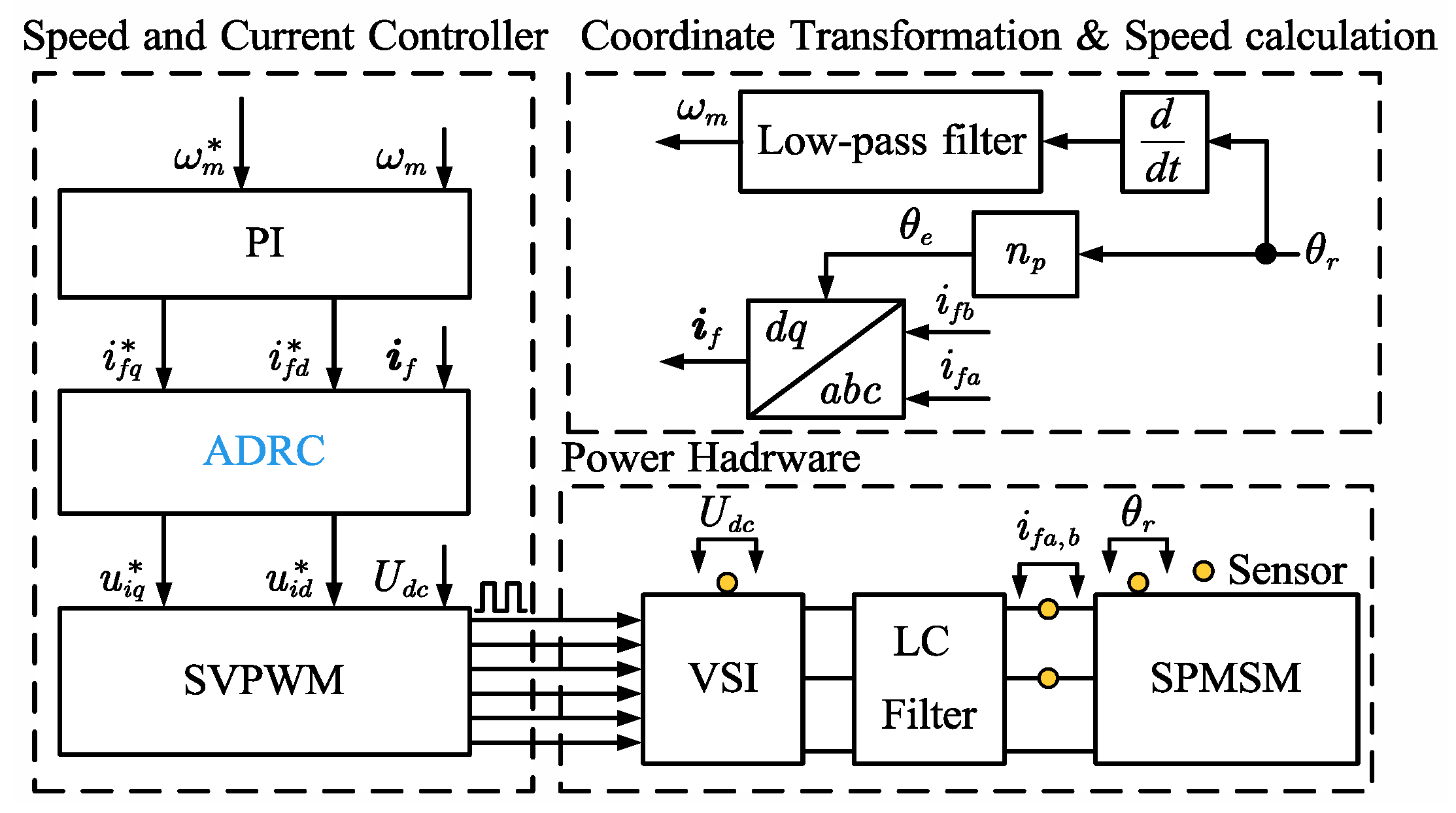
2. Modeling of LC-Filtered SPMSM Drive System and Traditional ADRC Design

2.1. Mathematical Modeling of System

The block diagram of the LC-filtered SPMSM drive system in the dq synchronous reference frame is shown in Figure 1, which includes the VSI, LC filter, and SPMSM. The output voltage and output current of VSI are defined as ${\mathit{u}}_i$ = $\left[u_{id},u_{iq}\right]$ and ${\mathit{i}}_i$ = $\left[i_{id},i_{iq}\right]$, respectively. The output voltage and output current of the LC filter are defined as ${\mathit{u}}_f$ = $\left[u_{fd},u_{fq}\right]$ and ${\mathit{i}}_f$ = $\left[i_{fd},i_{fq}\right]$, respectively. The LC filter is composed of the filter inductance $L_f$, the filter resistance $R_f$, and the filter capacitor $C_f$. The SPMSM parameters include stator inductance $L_s$, stator resistance $R_s$, electrical angular velocity ${\omega }_e$, pole pairs $n_p$ and permanent magnet flux linkage ${\psi }_m$.

Modeling the LC-filtered SPMSM drive system in the dq synchronous reference frame gives [13]

$$\left\{\begin{array}{c}{u}_{id}=L_f\left(d{i}_{id}/dt\right)+R_f{i}_{id}-{\omega }_e{L}_f{i}_{iq}+u_{fd}\\ u_{iq}=L_f\left(d{i}_{iq}/dt\right)+R_f{i}_{iq}+{\omega }_e{L}_f{i}_{id}+u_{fq}\end{array}\right.$$

(1)

$$\left\{\begin{array}{c}{i}_{id}=C_f\left(d{u}_{fd}/dt\right)-{\omega }_e{C}_f{u}_{fq}+i_{fd}\\ i_{iq}=C_f\left(d{u}_{fq}/dt\right)+{\omega }_e{C}_f{u}_{fd}+i_{fq}\end{array}\right.$$

(2)

$$\left\{\begin{array}{c}{u}_{fd}=L_s\left(d{i}_{fd}/dt\right)+R_s{i}_{fd}-{\omega }_e{L}_s{i}_{fq}\\ u_{fq}=L_s\left(d{i}_{fq}/dt\right)+R_s{i}_{fq}+{\omega }_e{L}_s{i}_{fd}+{\omega }_e{\psi }_m\end{array}\right.$$

(3)

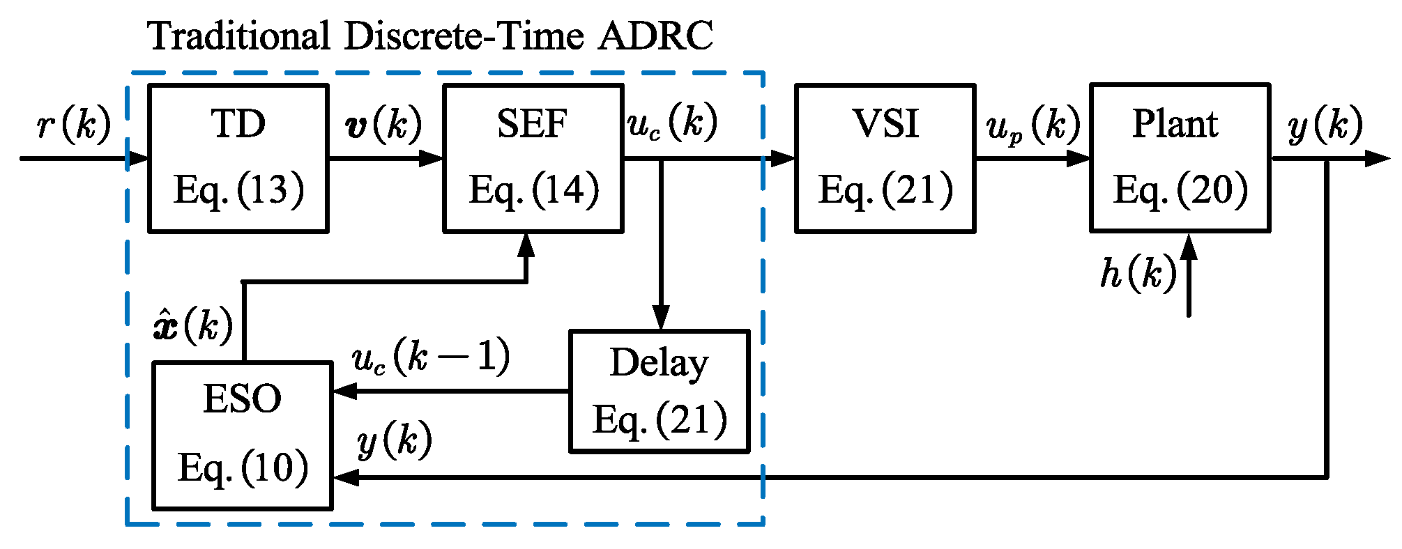
2.2. Design of the Third-Order ADRC in Continues Domain

The control block diagram of the LC-filtered SPMSM drive system is shown in Figure 2. The speed loop is based on the classical PI control, and the current loop is based on the third-order ADRC.

The design of the third-order ADRC in continuous domain includes extended state observer (ESO), tracking differentiator (TD) and state error feedback (SEF). ESO plays a very important role, relying on system model information for state variable estimation and disturbance rejection. TD is used to generate the reference signal traces. SEF is used to generate control signals with desired controller bandwidth.

Taking q axis as an example, substituting the differential of (1) and (2) into (3) yields the third-order expression of the q-axis LC filter output current as

$$\stackrel{⃛}{y}\left(t\right)=-a_2\ddot{y}\left(t\right)-a_1\dot{y}\left(t\right)-a_{0}y\left(t\right)+b_0{u}_p\left(t\right)+f_l\left(t\right)$$

(4)

where

$$\begin{gathered} a_0=\left(R_s+R_f\right)/\left(C_f{L}_f{L}_s\right);a_1=\left(L_f+L_s\right)/\left(C_f{L}_f{L}_s\right) \\ {a}_2=\left(C_f{L}_f{R}_s+C_f{L}_s{R}_f\right)/\left(C_f{L}_f{L}_s\right);b_0=1/\left(C_f{L}_f{L}_s\right). \end{gathered}$$

$y=i_{fq}$ is the q-axis current, $u_p=u_{iq}$ is the q-axis input voltage, and the number of dots above a letter represents the order of its time derivative. $f_l\left(t\right)$ represents the lumped disturbance of the system, which includes the back electromotive force, the dq-axis coupling, and the unmodeled dynamics.

An extended state is added to describe the dynamic of lumped disturbance in the system (4), thus the state-space expression of the extended system is noted as

$$\left\{\begin{array}{c}\dot{\mathit{x}}\left(t\right)={\mathit{A}}_p\mathit{x}\left(t\right)+{\mathit{B}}_p{u}_p\left(t\right)+\mathit{E}h\left(t\right)\\ y\left(t\right)=\mathit{C}\mathit{x}\left(t\right)\end{array}\right.$$

(5)

where

$$\mathit{x}\left(t\right)=\left[\begin{array}{c}{x}_1\left(t\right)\\ x_2\left(t\right)\\ x_3\left(t\right)\\ x_4\left(t\right)\end{array}\right];{\mathit{A}}_p=\left[\begin{array}{cccc}0& 1& 0& 0\\ 0& 0& 1& 0\\ 0& 0& 0& 1\\ 0& -a_0& -a_1& -a_2\end{array}\right];{\mathit{B}}_p=\left[\begin{array}{c}0\\ 0\\ b_0\\ -a_2{b}_0\end{array}\right];\mathit{E}=\left[\begin{array}{c}0\\ 0\\ 0\\ 1\end{array}\right];\mathit{C}={\left[\begin{array}{c}1\\ 0\\ 0\\ 0\end{array}\right]}^T.$$

$y\left(t\right)=i_{fq}\left(t\right)$ is the q-axis output current of LC filter, $u_p\left(t\right)$ is the system plant input, and $h\left(t\right)={\dot{f}}_l\left(t\right)$ is the derivative of the lumped disturbance.

The design of ESO is well-established in the continuous domain based on the extended system (5). With the observer gain matrix to correct the estimated states, the state-space expression of ESO is constructed as

$$\dot{\widehat{\mathit{x}}}\left(t\right)={\mathit{A}}_e\widehat{\mathit{x}}\left(t\right)+{\mathit{B}}_e{u}_e\left(t\right)+{\mathit{L}}_c\left(y\left(t\right)-\mathit{C}\widehat{\mathit{x}}\left(t\right)\right)$$

(6)

with $\widehat{\mathit{x}}\left(t\right)={\left[\begin{array}{cccc}{\widehat{x}}_1\left(t\right)& {\widehat{x}}_2\left(t\right)& {\widehat{x}}_3\left(t\right)& {\widehat{x}}_4\left(t\right)\end{array}\right]}^T$, ${\mathit{A}}_e={\mathit{A}}_p$, ${\mathit{B}}_e={\mathit{B}}_p$. ${\mathit{L}}_{\mathit{c}}$ is the observer gain matrix in continuous domain, $u_e$ is the input of ESO.

TD can be designed as

$$\dot{\mathit{v}}\left(t\right)={\mathit{A}}_t\mathit{v}\left(t\right)+{\mathit{B}}_{t}r\left(t\right)$$

(7)

where

$$\mathit{v}\left(t\right)=\left[\begin{array}{c}{v}_1\left(t\right)\\ v_2\left(t\right)\\ v_3\left(t\right)\end{array}\right];{\mathit{A}}_t=\left[\begin{array}{ccc}0& 1& 0\\ 0& 0& 1\\ -{\omega }_t^3& -3{\omega }_t^2& -3{\omega }_t\end{array}\right];{\mathit{B}}_t=\left[\begin{array}{c}0\\ 0\\ {\omega }_t^3\end{array}\right].$$

$\mathit{v}\left(t\right)$ is the reference signal traces matrix, ${\omega }_t$ is the tracking bandwidth, and $r\left(t\right)$ is the current-loop reference.

SEF is designed as

$$u_c\left(t\right)={\mathit{K}}_v\mathit{v}\left(t\right)-{\mathit{K}}_x\widehat{\mathit{x}}\left(t\right)$$

(8)

where control gains ${\mathit{K}}_v$ and ${\mathit{K}}_x$ are determined by bandwidth method commonly adopted in [32] as

$${\mathit{K}}_v=\left[\begin{array}{ccc}{\omega }_c^3& 3{\omega }_c^2& 3{\omega }_c\end{array}\right]/b_0;{\mathit{K}}_x=\left[\begin{array}{ccc}{\omega }_c^3& 3{\omega }_c^2& 3{\omega }_c\end{array} 1\right]/b_0.$$

(9)

2.3. Limitations of Euler Discretion and Current Observer

The control block diagram is shown in Figure 3. Based on the work of [37] on discrete ESO, the current observer form ESO is adopted as

$$\left\{\begin{array}{c}\overline{\mathit{x}}\left(k\right)={\overline{\mathit{\Phi }}}_e\widehat{\mathit{x}}\left(k-1\right)+{\overline{\mathit{\Gamma }}}_e{u}_p\left(k-1\right)\\ \widehat{\mathit{x}}\left(k\right)=\overline{\mathit{x}}\left(k\right)+{\overline{\mathit{L}}}_d\left(y\left(k\right)-\mathit{C}\overline{\mathit{x}}\left(k\right)\right)\end{array}\right.$$

(10)

where $k$ denotes the value at the time $t=kT$. $\overline{\mathit{x}}\left(k\right)$ is the predicted value obtained from the assumed plant dynamics. ${\overline{\mathit{\Phi }}}_e$ and ${\overline{\mathit{\Gamma }}}_e$ are the discrete dynamic matrices of the assumed plant. $u_p\left(k-1\right)$ is the input to the ESO, which is equal to $u_c\left(k-2\right)$. $\widehat{\mathit{x}}\left(k\right)$ is the corrected value derived from $\overline{\mathit{x}}\left(k\right)$ and the plant output $y\left(k\right)$. ${\overline{\mathit{L}}}_d$ is the observer gain matrix.

Using Euler discretization [38], the values of ${\overline{\mathit{\Phi }}}_e$ and ${\overline{\mathit{\Gamma }}}_e$ are derived as

$${\overline{\mathit{\Phi }}}_e={\mathit{I}}_4+T{\mathit{A}}_e;{\overline{\mathit{\Gamma }}}_e=T{\mathit{B}}_e.$$

(11)

The poles are then configured in the discrete domain to determine ${\overline{\mathit{L}}}_d$ as

$$\left|z{\mathit{I}}_4-\left({\overline{\mathit{\Phi }}}_e-{\overline{\mathit{L}}}_d\mathit{C}{\overline{\mathit{\Phi }}}_e\right)\right|={\left(z-z_o\right)}^4$$

(12)

where ${\mathit{I}}_4$ is a fourth-order identity matrix, $z$ is a Z-transform operator, $z_o=\mathrm{e}\mathrm{x}\mathrm{p}\left(-{\omega }_o{T}_s\right)$ is the poles of the observer in discrete domain.

TD (7) can be discretized by Euler method as

$$\widehat{\mathit{v}}\left(k\right)={\overline{\mathit{\Phi }}}_t\widehat{\mathit{v}}\left(k-1\right)+{\overline{\mathit{\Gamma }}}_{t}r\left(k-1\right)$$

(13)

where ${\overline{\mathit{\Phi }}}_t={\mathit{I}}_3+T{\mathit{A}}_t$, ${\overline{\mathit{\Gamma }}}_t=T{\mathit{B}}_t$, ${\mathit{I}}_3$ is a third-order identity matrix, and $r\left(k\right)$ is the reference signal of current loop.

SEF (8) can be discretized naturally as

$$u_c\left(t\right)={\mathit{K}}_v\mathit{v}\left(k\right)-{\mathit{K}}_x\widehat{\mathit{x}}\left(k\right).$$

(14)

The traditional discrete methods mentioned above mainly suffer from two issues: discretization inaccuracies and the impact of one-beat time delay.

Backward Euler discretization introduces errors between the real system model and the ESO. These errors increase as the switching frequency decreases, potentially leading to resonance peaks and additional phase lag.

The one-beat computation delay in digital control systems significantly impacts system stability by reducing the phase margin. In the frequency domain, this delay introduces frequency-dependent phase lag that increases proportionally with frequency.

Consequently, the combined effects of discretization inaccuracies and the one-beat time delay diminish the stability margin of ADRC implemented with Euler discretization and the current-observer method. Therefore, when attempting to improve dynamic performance, the system can easily become unstable. This can be observed in the variation of the closed-loop poles shown in Figure 4. The range of control bandwidth ${\omega }_c$ varies from 50 Hz to 500 Hz, with a step size of 50 Hz, while ${\omega }_o$ is fixed at 1500 Hz. The system parameters used in this analysis are consistent with those listed in Table 3 of Section 5. As the control bandwidth ${\omega }_c$ increases, the poles in Figure 3 gradually shift from inside the stable unit circle to outside the unstable unit circle. The system becomes unstable around at ${\omega }_c$ = 250 Hz. The detailed derivation is conducted in Section 4.

3. Proposed Predictive ESO for Delay Compensation and ZOH Accurate Discretization

Discretization inaccuracies and one-beat time delays reduce controller bandwidth and degrade dynamic performance. In this section, an accurate discretization and delay-compensated method are proposed to address this issue.

3.1. Accurate Plant Discretization via ZOH Method

The discrete observer (10) can be divided into two parts:

one part is the observer dynamics item which simulates the system dynamics, represented as ${\overline{\mathit{\Phi }}}_e\widehat{\mathit{x}}\left(k-1\right)+{\overline{\mathit{\Gamma }}}_e{u}_p\left(k-1\right)$. When the ${\overline{\mathit{\Phi }}}_e$ and ${\overline{\mathit{\Gamma }}}_e$ matrices of the observer closely match those of the real plant, the system’s stability margin is higher, allowing for greater dynamic response.

The other part is the correction item based on the feedback value, represented as ${\overline{\mathit{L}}}_d\left(y\left(k\right)-\mathit{C}\overline{\mathit{x}}\left(k\right)\right)$.The selection and impact of ${\overline{\mathit{L}}}_d$ will be analyzed in the next subsection.

Compared to the Euler discretization method, the ZOH discretization method can more accurately obtain the plant’s dynamic matrices under PWM voltage input. The core concept of ZOH discretization is to assume that the plant’s input remains constant during each sampling interval. Simultaneously, the PWM output is approximated as a constant value within each interval, following the volt-second balance principle [41]. The following is the derivation process.

According to the solution of state-space Equation (5), state variables at instant $t=kT$ and $t=\left(k+1\right)T$ are obtained as

$$\mathit{x}\left(k\right)=e^{{\mathit{A}}_{p}kT}\mathit{x}\left(0\right)+e^{{\mathit{A}}_{p}kT}{\int }_0^{kT}{e}^{-{\mathit{A}}_p\tau }\left({\mathit{B}}_p{u}_p\left(\tau \right)+\mathit{E}h\left(\tau \right)\right)d\tau$$

(15)

$$\mathit{x}\left(k+1\right)=e^{{\mathit{A}}_p\left(k+1\right)T}\mathit{x}\left(0\right)+e^{{\mathit{A}}_p\left(k+1\right)T}{\int }_0^{\left(k+1\right)T}{e}^{-{\mathit{A}}_p\tau }\left({\mathit{B}}_p{u}_p\left(\tau \right)+\mathit{E}h\left(\tau \right)\right)d\tau$$

(16)

Multiply (15) by $\mathrm{e}\mathrm{x}\mathrm{p}\left({\mathit{A}}_{p}T\right)$, and then subtract Equation (16) to obtain:

$$\mathit{x}\left(k+1\right)=e^{{\mathit{A}}_{p}T}\mathit{x}\left(k\right)+e^{{\mathit{A}}_p\left(k+1\right)T}{\int }_{kT}^{\left(k+1\right)T}{e}^{-{\mathit{A}}_p\tau }\left({\mathit{B}}_p{u}_p\left(\tau \right)+\mathit{E}h\left(\tau \right)\right)d\tau$$

(17)

The PWM output voltage $u_p\left(t\right)$ between $kT$ and $\left(k+1\right)T$ can be approximated as a zero-order holder, which can be expressed as

$$u_p\left(t\right)=u_p\left(k\right),h\left(t\right)=h\left(k\right)\left(kT⩽t<kT+T\right).$$

(18)

According to the ZOH characteristics, (17) can be simplified as

$$\begin{array}{ll}\mathit{x}\left(k+1\right)=e^{{\mathit{A}}_{p}T}& \mathit{x}\left(k\right)+e^{{\mathit{A}}_{p}T}{\int }_0^T{e}^{-{\mathit{A}}_{p}t}\left({\mathit{B}}_p{u}_p\left(k\right)+\mathit{E}h\left(k\right)\right)dt\\ & =e^{{\mathit{A}}_{p}T}\mathit{x}\left(k\right)+{\int }_0^T{e}^{{\mathit{A}}_p\lambda }\left({\mathit{B}}_p{u}_p\left(k\right)+\mathit{E}h\left(k\right)\right)d\lambda \end{array}$$

(19)

where $\lambda =T-t$.

The discrete state equation of the plant based ZOH method is listed as

$$\left\{\begin{array}{c}\mathit{x}\left(k+1\right)={\mathit{\Phi }}_p\mathit{x}\left(k\right)+{\mathit{\Gamma }}_p{u}_p\left(k\right)+{∆}_{p}h\left(k\right)\\ y\left(k\right)=\mathit{C}\mathit{x}\left(k\right)\end{array}\right.$$

(20)

where ${\mathit{\Phi }}_p=e^{{\mathit{A}}_{p}T};{\mathit{\Gamma }}_p=\left({\int }_0^T{e}^{{\mathit{A}}_p\tau }d\tau \right){\mathit{B}}_p;{∆}_p=\left({\int }_0^T{e}^{{\mathit{A}}_p\tau }d\tau \right)\mathit{E}$.

The plant’s precise discrete model, obtained using the ZOH method, as given in (20), serves as the basis for designing the discrete ESO. The dynamic process of the discrete ESO designed based on (20) closely mimics the dynamics of the plant, thereby improving the system’s stability margin.

3.2. Improved Predictive ESO with One-Beat Lead

In addition to obtaining the plant’s accurate discrete dynamic model through the ZOH method, the ESO also needs to be improved to account for the one-beat time delay introduced by digital computation.

Time delay is noted in discrete domain as

$$G_d\left(z\right)=z^{-1}$$

(21)

The current observer, as shown in (10), provides the estimate at the current time $t=kT$, and it does not compensate for the one-beat time delay. Similarly, the traditional predictive observer, as illustrated by the dashed line in Figure 5, outputs the state estimate to the SEF, which is still based on the current time $t=kT$. In addition, since the traditional predictive observer uses $u_p\left(k-1\right)$ and $y\left(k-1\right)$ to calculate $\widehat{\mathit{x}}\left(k\right)$, this method theoretically introduces a greater delay compared to the current observer.

This paper proposes an improved predictive observer that provides a one-step lead prediction, outputting the predicted value at time $t=\left(k+1\right)T$, which helps to counteract the one-beat delay in the forward channel. The proposed control method is shown in Figure 5 based on ADRC using the improved predictive ESO and accurate ZOH discretization.

The proposed predictive ESO based on the ZOH discretization method is given by

$$\widehat{\mathit{x}}\left(k+1\right)={\mathit{\Phi }}_e\widehat{\mathit{x}}\left(k\right)+{\mathit{\Gamma }}_e{u}_e\left(k\right)+{\mathit{L}}_d\left(y\left(k\right)-\mathit{C}\widehat{\mathit{x}}\left(k\right)\right)$$

(22)

where ${\mathit{\Phi }}_e={\mathit{\Phi }}_{\begin{array}{c}p\end{array}};{\mathit{\Gamma }}_e={\mathit{\Gamma }}_p$.

The SEF based on the proposed predictive ESO is given by

$$u_c\left(k\right)={\mathit{K}}_v\mathit{v}\left(k+1\right)-{\mathit{K}}_x\widehat{\mathit{x}}\left(k+1\right)$$

(23)

Subtracting the observer equation from the state equation with $\mathit{e}\left(k\right)=\mathit{x}\left(k\right)-\widehat{\mathit{x}}\left(k\right)$ yields

$$\mathit{e}\left(k+1\right)=\left({\mathit{\Phi }}_e-{\mathit{L}}_d\mathit{C}\right)\mathit{e}\left(k\right)$$

(24)

Based on the above equation, the dynamics of the error can be designed in the discrete domain. The observer feedback gain matrix ${\mathit{L}}_d$ is derived as

$$\mathrm{d}\mathrm{e}\mathrm{t}\left(z{\mathit{I}}_4-\left({\mathit{\Phi }}_e-{\mathit{L}}_d\mathit{C}\right)\right)={\left(z-z_o\right)}^4$$

(25)

where $z_o=e^{-{\omega }_{o}T}$ is parameter related to observer bandwidth, and $z_o$ is the mapping point of ${\omega }_o$ in $z$ domain.

To verify the improvement in dynamic performance of the ADRC based on the ZOH discretization method and the improved predictive observer, the closed-loop pole trajectories are illustrated in Figure 6. The control bandwidth ${\omega }_c$ varies from 350 Hz to 800 Hz, with a step size of 50 Hz, while the observer bandwidth ${\omega }_o$ is fixed at 1500 Hz. It can be seen that when the controller bandwidth reaches 800 Hz, the system’s closed-loop poles remain inside the unit circle. In comparison to the ADRC based on the Euler discretization method and the conventional observer shown in Figure 4, the controller bandwidth can be significantly increased without losing stability.

4. Robust Control Parameter Design Based on Open-Loop Transfer Function Margin Metrics

Predictive control strategies typically require rigorous stability analysis, and the proposed discrete ESO is no exception. This section presents a systematic approach for control parameter design based on margin metrics, aiming to achieve a trade-off between robustness and dynamic.

4.1. Open-Loop Transfer Function Derivation

The equivalent control block of the control system is derived as shown in Figure 7. ${\mathit{G}}_t\left(z\right)$ is the transfer function of TD derived in Section 4.3.

Based on the discrete expression of ESO in (22), the relation between the estimated state vector $\widehat{\mathit{X}}\left(z\right)$ and the input of ESO $U_e\left(z\right)$ and $Y\left(z\right)$ is obtained as

$$\widehat{\mathit{X}}\left(z\right)={\mathit{G}}_1\left(z\right)U_e\left(z\right)+{\mathit{G}}_2\left(z\right)Y\left(z\right)$$

(26)

where uppercase letters denote variables in the Z-domain; for example, $Y\left(z\right)$ is the Z-transform of $y\left(k\right)$. The transfer function is defined as follows:

$${\mathit{G}}_1\left(z\right)={\left(z{\mathit{I}}_4-{\mathit{\Phi }}_{\mathit{e}}+{\mathit{L}}_d\mathit{C}\right)}^{-1}{\mathit{\Gamma }}_e; {\mathit{G}}_2\left(z\right)={\left(z{\mathit{I}}_4-{\mathit{\Phi }}_e+{\mathit{L}}_d\mathit{C}\right)}^{-1}{\mathit{L}}_d.$$

The Z-transform of the ESO output $\widehat{\mathit{x}}\left(k+1\right)$ is

$$\mathcal{Z}\left[\widehat{\mathit{x}}\left(k+1\right)\right]=z\widehat{\mathit{X}}\left(z\right)$$

(27)

where $\mathcal{Z}$ represents the Z-transform.

The modeling of plant in discrete domain with ZOH input according to (20) is obtained as

$$G_p\left(z\right)=Y\left(z\right)/U_p\left(z\right)=\mathit{C}{\left(z{\mathit{I}}_4-{\mathit{\Phi }}_p\right)}^{-1}{\mathit{\Gamma }}_p.$$

(28)

The open-loop transfer function of the control system is obtained as

$$G_{op}\left(z\right)=U_c\left(z\right)/M\left(z\right)={\mathit{K}}_x\left({\mathit{G}}_1\left(z\right)+G_p\left(z\right){\mathit{G}}_2\left(z\right)\right).$$

(29)

4.2. Control Parameters Design and Margins Improvement

Increased control bandwidth ${\omega }_c$ enhances the system’s dynamic response performance and disturbance rejection capability. However, excessively high bandwidth ${\omega }_c$ may compromise system robustness, creating an inherent trade-off between dynamic response and stability.

Based on frequency-domain design principles, the open-loop transfer function must satisfy the following stability criteria to ensure both dynamic performance and robustness:

• A minimum phase margin of 40°.
• A minimum gain margin of 6 dB.

Following these design guidelines, the proposed improved discrete ADRC parameters are selected as

$${\omega }_c=500 \mathrm{Hz}; {\omega }_o=3{\omega }_c=1500\mathrm{Hz}$$

(30)

Figure 8 shows the Bode plots of the open-loop transfer functions for the four discretization methods of “Euler discretization + Current observer” (“Eul. + Cur.”), “ZOH discretization + improved predictive observer” (“ZOH + Pre.”), “Euler discretization + improved predictive observer” (“Eul. + Pre.”), and “ZOH discretization + Current observer” (“ZOH + Cur.”). The control bandwidth is set as ${\omega }_c$ = 500 Hz, and the ESO bandwidth is set as ${\omega }_o$ = 1500 Hz.

As illustrated in Figure 8, the proposed “ZOH + Pre.” method achieves a gain margin of 6.3 dB and a phase margin of 63.8°, demonstrating high stability margins and meeting robustness requirements. In contrast, the “Eul. + Pre.” method yields a gain margin of 5.3 dB and a phase margin of 18.5°, indicating relatively lower stability margins and insufficient robustness. The “ZOH + Cur.” method further degrades, with a gain margin of 0.4 dB and a phase margin of 3.3°, approaching the stability boundary. Notably, the “Eul. + Cur.” method fails to maintain stability, exhibiting a gain margin of −10.3 dB and a phase margin of −73.5°. The proposed “ZOH + Pre.” method significantly enhances system stability, improving the gain margin from −10.3 dB to 6.3 dB (a 16.6 dB increase) and the phase margin from −73.5° to 63.8° (a 137.3° increase).

It can be concluded that, under the same bandwidth, both the improved predictive observer method and the ZOH discretization can improve the gain margin and phase margin, compared to the current observer method and the Euler discretization. As a result, it offers a significant advantage when increasing the controller bandwidth to improve system dynamic performance. This alleviates the trade-off between system dynamic performance and robustness, ensuring stability at higher control bandwidths.

4.3. Tracking Differentiator and Step Response

While the open-loop transfer function determines the stability margin of the control system, it is the closed-loop transfer function that critically defines the system’s tracking performance.

TD (7) can be discretized by ZOH method as

$$\widehat{\mathit{v}}\left(k\right)={\mathit{\Phi }}_t\widehat{\mathit{v}}\left(k-1\right)+{\mathit{\Gamma }}_{t}r\left(k-1\right)$$

(31)

where ${\mathit{\Phi }}_t=e^{{\mathit{A}}_{t}T};{\mathit{\Gamma }}_t=\left({\int }_0^T{e}^{{\mathit{A}}_t\tau }d\tau \right){\mathit{B}}_t.$ The transfer function of the TD in the discrete domain is denoted as

$${\mathit{G}}_{\mathit{t}}\left(z\right)={\left(z{\mathit{I}}_3-{\mathit{\Phi }}_t\right)}^{-1}{\mathit{\Gamma }}_t.$$

(32)

Design of bandwidth parameter for TD is based on the engineering configuration experience as

$${\omega }_t=2{\omega }_c.$$

(33)

Based on Figure 7, the closed-loop transfer function of the control system is hence derived as

$$G_{cl}\left(z\right)={\displaystyle \frac{R\left(z\right)}{Y\left(z\right)}}={\displaystyle \frac{{\mathit{K}}_v{\mathit{G}}_{\mathit{t}}\left(z\right)G_p\left(z\right)}{1+G_{op}\left(z\right)}}.$$

(34)

The selection of controller and observer bandwidth parameters must consider the phase margin of the system’s open-loop transfer function. Insufficient phase margin (typically < 40°) indicates proximity to instability, particularly under parameter uncertainties. Practical control methods therefore require adequate phase margin.

As Figure 8 demonstrates, the “Eul. + Pre.”, “Eul. + Cur.”, and “ZOH + Cur.” methods exhibit critically low phase margins (<20°) at ${\omega }_c$ = 500 Hz and ${\omega }_o$ = 1500 Hz, rendering them unsuitable for direct implementation. Mitigation involves reducing controller and observer bandwidths to enhance phase margins.

Table 1. Phase margins with reduced controller and observer bandwidth.

Methods	Control Bandwidth and Observer Bandwidth	Phase Margin	Reduced Bandwidth	Phase Margin
“ZOH + Pre.”	500 Hz; 1500 Hz	63.8°	No need to reduce bandwidth
“Eul. + Pre.”	500 Hz; 1500 Hz	18.5°	300 Hz; 600 Hz	41.2°
“ZOH + Cur.”	500 Hz; 1500 Hz	3.3°	300 Hz; 600 Hz	40.1°
“Eul. + Cur.”	500 Hz; 1500 Hz	−73.5°	150 Hz; 600 Hz	34.5°

quantifies the improved phase margins with reduced controller and observer bandwidths.

For TD bandwidth selection, empirical practice suggests setting it to twice the controller bandwidth in (33) to accelerate closed-loop response.

The resulting parameter configurations for different discretization methods are detailed in

Table 2. Selection of bandwidth parameters for step response.

Methods	$\mathbf{Control} \mathbf{Bandwidth} {\mathit{\omega }}_{\mathit{c}}$	$\mathbf{Observer} \mathbf{Bandwidth} {\mathit{\omega }}_{\mathit{o}}$	$\mathbf{TD} \mathbf{Bandwidth} {\mathit{\omega }}_{\mathit{t}}$
“ZOH + Pre.”	500 Hz	1500 Hz	1000 Hz
“Eul. + Pre.”	300 Hz	600 Hz	600 Hz
“ZOH + Cur.”	300 Hz	600 Hz	600 Hz
“Eul. + Cur.”	150 Hz	600 Hz	300 Hz

, with numerical calculation of step response shown in Figure 9. For “ZOH + Pre.” method, the settling time is 1.0 ms with an overshoot of 1%. “Eul. + Pre.” method shows a settling time of 2.6 ms and an overshoot of 13%. For “Eul. + Cur.” method, the settling time is 6.2 ms with an overshoot of 11%, while “ZOH + Cur.” method has a settling time of 9.6 ms and an overshoot of 4%.

With the inclusion of accurate discretization and delay compensation, both the settling time and overshoot improve in current tracking performance.

5. Experimental Verification

The effectiveness of the proposed method was validated experimentally. All control parameters used in the experimental verification are listed in Table 2. The experimental setup of the drive system is shown in Figure 10. The basis for the design and selection of LC filters can be seen in [4]. The experiments were conducted using a dSPACE MicroLabBox (ds1202) real-time platform along with the hardware prototype. The system parameters are listed in

Table 3. Parameters of system.

Symbol	Parameter	Value
$L_f$	Inductance of filter	2.2 mH
$R_f$	Resistance of filter	$0.5 \mathsf{\Omega }$
$C_f$	Capacitor of filter	$11 \mathsf{\mu }\mathrm{F}$
$L_s$	Inductance of SPMSM	6.5 mH
$R_s$	Resistance of stator	$1 \mathsf{\Omega }$
$n_p$	Number of pole pairs	4
${\psi }_m$	Motor flux linkage	0.086 Wb
$I_n$	Rated motor current	3.5 A
$P_n$	Rated motor power	750 W
$n_n$	Rated rotor speed	1500 r/min
$J$	System moment of inertia (with load)	0.005 kg·m2
$U_{dc}$	DC-link voltage	311 V
$f_s$	Sampling and Switching frequency	10 kHz

. The system is powered by a 311 V DC source, making it suitable for industrial applications. The sampling rate and control frequency are both set to 10 kHz, with the inverter dead-time set to 1 μs. The LC filter consists of three-phase inductors and capacitors. The SPMSM is connected to a magnetic powder brake, which serves as the load via a shaft.

The output voltage of the LC filter and the DC bus voltage were measured by Hall-effect voltage sensors (LEM LV 25-P). The SPMSM are configured with the parameters specified in Table 3. The output current of the LC filter was measured by Hall-effect current sensors (LEM LA 25-P). The SPMSM is equipped with a high-resolution incremental encoder with 2500 pulses per revolution to ensure accurate position feedback. These measurement signals are fed into the dSPACE system, which generates PWM signals for driving the inverter through the control strategy.

5.1. Speed and Current Response During Startup

Figure 11 shows the rotor speed, and motor current waveforms during the startup process of the SPMSM. Both the “ZOH + Pre.” and “Eul. + Cur.” discretization methods were applied to discretize the ADRC in the current controller. Control parameters are selected from Table 2. Both speed controllers employ conventional PI control with a bandwidth set to 5 Hz. An enlarged version of the current waveforms is also provided to observe more details of the dynamic process during the current step response.

Figure 11a shows the motor speed waveform during startup, with the speed reference value stepping from 0 to 1000 r/min at 0 s. The rotor speed settling time (5%) for both “ZOH + Pre.” and “Eul. + Cur.” discretization methods are close to 210 ms.

Figure 11b shows the current waveform during the startup process. The steady-state current fluctuation amplitude for the “ZOH + Pre.” discretization method is 0.5 A (10% of reference current), while for the “ZOH + Pre.” discretization method, it is 2.2 A (44% of reference current).

Figure 11c shows more details of the current step response at zero speed. The current settling time (5%) of the “ZOH + Pre.” discretization method is 1.1 ms with no overshoot, compared to 10.0 ms with a 4% overshoot for the “Eul. + Cur.” discretization method. The experimental current step response waveforms closely match the numerical calculation results shown in Figure 9.

Therefore, the proposed “ZOH + Pre.” discretization method significantly outperforms the “Eul. + Cur.” discretization method in terms of current settling time, highlighting the effectiveness and necessity of accurate discretization and delay compensation techniques in applications demanding fast dynamic responses.

5.2. Current Step Responses of Proposed Discretization Method at Different Rotor Speeds

Figure 12a–d show the motor current step response of the proposed discretization ADRC at different rotor speeds: 375 r/min (25 Hz), 750 r/min (50 Hz), 1125 r/min (75 Hz), and 1500 r/min (100 Hz). It is noteworthy that the current response shown in Figure 11c can be approximately considered at a rotor speed of 0 r/min (0 Hz). At different rotor speed, a 5A (rated current) step signal is applied to the q-axis current reference of the SPMSM at 0 s.

The integral of the time multiplied by the absolute error (ITAE) index is commonly used to evaluate the tracking dynamic performance, and it is defined as

$$\mathrm{I}\mathrm{T}\mathrm{A}\mathrm{E}\left(y^{\mathrm{*}},y\right)=\sqrt{\sum _{k=1}^m\left(kT|y^{\mathrm{*}}\left(k\right)-y\left(k\right)|\right)}$$

(35)

where $y^{\mathrm{*}}$ is the reference value, $y$ is the actual value, $m$ is the number of points in the selected interval, $T$ is the sampling time, $y^{\mathrm{*}}\left(k\right)$ and $y\left(k\right)$ are the value of $y^{\mathrm{*}}$ and $y$, respectively, at time $k$.

Based on Figure 12 and Figure 11c, the settling time of motor current with the proposed discretization method is 1.1 ms for frequencies ranging from 0 Hz up to 75 Hz and 1.3 ms at 100 Hz. The overshoot increases slightly with rotor speed, rising from 0.3% to 2.5%. In the interval [0 ms, 3.5 ms], the ITAE increases slightly by 0.005 for frequencies exceeding 25 Hz, while maintaining a baseline value of 0.0109 at zero speed. These results indicate that the current dynamic performance remains similar to the zero-speed condition when the rotational speed operates below the fundamental frequency. The increased settling time and ITAE observed at higher speeds during dynamic processes are likely attributable to the increased back electromotive force and dq-axis coupling.

5.3. Comparison of Closed-Loop Performance with Different Discretization Methods

This section validates the improvement in dynamic performance of the current loop achieved by the proposed precise discretization and delay compensation method, compared to traditional discretization methods, through both frequency-domain Bode plots and time-domain step response analysis.

(a)

Frequency-domain: closed-loop frequency sweep with different discretization methods

Figure 13 presents the closed-loop Bode plots in the frequency domain for different discretization methods, with the speed condition set to 0 r/min. The frequency sweep is conducted using a chirp signal in the range of 10–1000 Hz as the reference signal. From this, the values of reference and feedback are obtained to derive the Bode plot of the closed-loop response. Bandwidth is commonly used as a metric to assess frequency-domain performance. The magnitude bandwidth is defined as the frequency at which the magnitude drops to −3 dB, while the phase bandwidth is the frequency at which the phase decreases to −45°.

From Figure 13, it can be seen that for “ZOH + Pre.” method, the magnitude bandwidth is 636 Hz, and the phase bandwidth is 200 Hz. For the “Eul. + Pre.” method, the magnitude bandwidth is 212 Hz, and the phase bandwidth is 116 Hz. The “Eul. + Cur.” method shows the magnitude bandwidth at 132 Hz and the phase bandwidth at 84 Hz, while the “ZOH + Cur.” method has the magnitude bandwidth at 45 Hz and the phase bandwidth at 30 Hz.

These results indicate that with precise discretization and delay compensation, the system’s bandwidth for tracking performance improves significantly. Specifically, the magnitude bandwidth is increased by a factor of 14.1, and the phase bandwidth is increased by a factor of 6.7.

(b)

Time-domain: step response with different discretization methods

Figure 14 illustrates the current step response in the time-domain for different discretization methods, with the speed condition again set to 0 r/min. For the “ZOH + Pre.” method, the settling time is 1.1 ms with almost no overshoot. The “Eul. + Pre.” method shows a settling time of 2.7 ms and an overshoot of 18%. For the “Eul. + Cur.” method, the settling time is 5.8 ms with an overshoot of 15%, while the “ZOH + Cur.” method has a settling time of 9.7 ms and an overshoot of 3%.

It is clear that, with the inclusion of precise discretization and delay compensation, both the settling time and overshoot improve in current tracking performance. Specifically, the settling time is reduced by 88% compared to traditional discrete methods. Furthermore, comparing the numerical calculations from Figure 9 with the experimental results in Figure 14, it is evident that the experimental outcomes are in good agreement with the theoretical predictions.

From both the frequency-domain and time-domain results, it is evident that the proposed discretization method significantly enhances dynamic performance and outperforms existing discretization methods.

5.4. Comparison with Existing Methods

To facilitate comparison with settling times obtained at different switching frequencies in different papers, the unit of settling time has been changed from milliseconds to the number of control periods in this subsection. This means that the settling periods are now expressed as the number of control periods required for the step response to reach a steady-state error of less than 5%. A lower settling period value indicates a quicker system response, making it a useful metric for evaluating the performance of control strategies with different switching periods.

The experimental data for MPC [7], AD [9], and TCPI [13] are extracted from their respective references. The experimental results of the proposed method are provided in Figure 14.

Table 4. Step response and sensors comparison with existing methods.

Methods	Settling Periods	Percentage of Overshoot	Voltage and Current Sensors
Proposed	11	Nearly 0%	Filter output current *2
MPC [7]	52	24%	Filter output current *2 Filter capacitor current *2 Inverter output current *2
AD [9]	40	30%	Filter output current *2
TCPI [13]	41	8%	Filter output current *2 Filter output voltage *2 Inverter output current *2
ADRC 1	97	2%	Filter output current *2

¹ The ADRC is based on the Euler discretization and current observer method in this paper. *2 means two sensors.

presents a comparison between the proposed method and existing methods in terms of settling periods, overshoot, and number of voltage and current sensors.

The proposed method demonstrates a significant advantage in current loop dynamic performance, with a settling time of 11 cycles and minimal overshoot. This method requires only two filter-output current sensors in addition to the DC-link voltage sensor. In contrast, the MPC [7] method exhibits a settling time of 52 cycles, an overshoot of 24%, and requires six sensors. The AD [9] method has a settling time of 40 cycles, an overshoot of 30%, and requires two sensors. The TCPI [13] method shows a settling time of 41 cycles, an overshoot of 8%, and requires six sensors. The Euler discretization and current observer method ADRC shows a settling time of 97 cycles, an overshoot of 3%, and requires two sensors.

The comparison with existing methods is summarized in Table 4. The proposed method reduces the settling time by over 72%, eliminates overshoot entirely, and requires the fewest sensors. These results demonstrate that the improved discrete-time ADRC method offers a remarkably fast dynamic response, and reduced hardware complexity.

5.5. Robustness Validation via Open-Loop Margins and Step Response Under Parameter Mismatches

This section validates the robustness of the proposed precise discretization and delay compensation method through both the open-loop transfer function and the step response under parameter mismatches.

(a)

Frequency-domain: open-loop transfer function frequency sweep

Figure 15 shows the frequency sweep results of the system’s open-loop transfer function. The sweep is conducted using a chirp signal in the range of 10–4000 Hz as the reference signal, from which the Bode plot of the open-loop transfer function in the frequency domain is derived. In Figure 15, the open-loop gain margin is 6.6 dB and the phase margin is 58.7°, which closely matches the theoretical values shown in Figure 8: 6.3 dB for the gain margin and 63.8° for the phase margin, with an error of less than 10%.

• (b) Time-domain: step response under parameter mismatches

Inductance may vary due to magnetic saturation, capacitance may deviate due to measurement errors, and resistance may change with temperature fluctuations. Therefore, this subsection involves the following parameter mismatches: filter inductance $L_f$, filter capacitance $C_f$, stator inductance $L_s$, and the total single-phase resistance $R$ (where $R=R_f+R_s$). The controller uses the values marked with a hat, while the unmarked values represent the actual system parameters.

Figure 16(a1,a2) shows the step response of the current under filter inductance mismatch. When ${\widehat{L}}_f=0.7L_f$, the current settling time is 2.1 ms, with an overshoot of 4.8%, and ITAE = 0.0164. When ${\widehat{L}}_f=1.3L_f$, the settling time is 2.5 ms, with an overshoot of 4.7%, and ITAE = 0.0177.

Figure 16(b1,b2) present the step response under filter capacitance mismatch. When ${\widehat{C}}_f=0.7C_f$, the settling time is 3.3 ms, with an overshoot of 5.5%, and ITAE = 0.0175. When ${\widehat{C}}_f=1.3C_f$, the settling time is 2.0 ms, with an overshoot of 3.5%, and ITAE = 0.0185.

Figure 16(c1,c2) illustrate the step response under stator inductance mismatch. When ${\widehat{L}}_s=0.7L_s$, the settling time is 1.8 ms, with an overshoot of 3.8%, and ITAE = 0.0228. When ${\widehat{L}}_f=1.3L_f$, the settling time is 2.4 ms, with an overshoot of 5.7%, and ITAE = 0.0192.

Figure 16(d1,d2) show the step response under total single-phase resistance mismatch. When $\widehat{R}=0.5R$, the settling time is 1.0 ms, with an overshoot of 4.4%, and ITAE = 0.0140. When $\widehat{R}=2R$, the settling time is 1.1 ms, with an overshoot of 4.9%, and ITAE = 0.0179.

When parameter mismatches of ±30% occur, the system remains stable. The maximum settling time is 3.1 ms, and the maximum overshoot is 5.5%, occurring when ${\widehat{C}}_f=0.7C_f$. The maximum ITAE occurs when ${\widehat{L}}_s=0.7L_s$, with a value of 0.0228. The method is not sensitive to variations in resistance, and the settling time remains nearly unchanged when resistance varies. To achieve the best dynamic performance, it is recommended to accurately measure the filter capacitance parameters and use look-up tables to handle the saturation characteristics of the inductance, while more relaxed tolerances can be applied to resistance values.

Thus, the control parameters designed based on the proposed frequency-domain margin metrics ensure good parameter robustness and maintain excellent dynamic performance, even under parameter mismatches.

5.6. Increasing and Reducing Load Torque

Figure 17 illustrates the speed and current variations during load torque application and shedding. Figure 17(a1,a2) depict the speed waveform and current profile when applying a 2 Nm load torque (80% of rated torque). Figure 17(b1,b2) show the corresponding responses during torque shedding from 2 N·m to 0. The waveforms validate that the proposed control method enables rapid tracking of the q-axis current reference during both loading and unloading transients.

5.7. Voltage and Current Characteristics at Inverter Output and LC Filter Output

Figure 18 demonstrates the voltage and current waveforms at inverter output and LC filter output under 50 Hz electrical frequency (750 r/min) at 80% rated load. Specifically, Figure 18a shows the inverter and filter output line voltage, while Figure 18b displays the inverter and filter output phase current. As shown in Figure 18a, the inverter output voltage exhibits a PWM waveform, while the filtered output voltage demonstrates a quasi-sinusoidal profile. Figure 18b reveals that the filter output current contains significantly reduced high-frequency components compared to the inverter output current, confirming the effective harmonic suppression capability of the LC filter. This results in motor terminal voltage and current waveforms closely approximating ideal sinusoidal characteristics.

6. Conclusions

This paper proposes an improved discrete-time ADRC strategy for fast and robust current control in LC-filtered SPMSM drive systems. The proposed strategy incorporates an accurate zero-order hold discretization method and an improved predictive observer, which significantly enhances the control system’s amplitude and phase margins over traditional Euler discretization and current observer. The control parameters are meticulously designed based on discrete-time frequency-domain metrics to ensure enhanced robustness. Experimental results demonstrate that the improved discrete-time ADRC strategy significantly improves the dynamic performance of motor current. It reduces the settling time by over 72% compared to existing methods, while also having enough robustness to handle common parameter mismatches.

The findings from this paper underscore the efficacy of accurate discretization and delay compensation, which could be instrumental in advancing ADRC for applications demanding high dynamic performance.

References

1. Yang, J.; Chen, W.H.; Li, S.; Guo, L.; Yan, Y. Disturbance/ uncertainty estimation and attenuation techniques in PMSM drives—A survey. IEEE Trans. Ind. Electron. 2017, 64, 3273–3285. [Google Scholar] [CrossRef]
2. Jiang, Y.; Wu, W.; He, Y.; Chung, H.S.; Blaabjerg, F. New passive filter design method for overvoltage suppression and bearing currents mitigation in a long cable based PWM inverter-fed motor drive system. IEEE Trans. Power Electron. 2017, 32, 7882–7893. [Google Scholar] [CrossRef]
3. Velander, E.; Bohlin, G.; Sandberg, A.; Wiik, T.; Botling, F.; Lindahl, M.; Zanuso, G.; Nee, H.-P. An ultralow loss inductorless dv/dt filter concept for medium-power voltage source motor drive converters with SiC devices. IEEE Trans. Power Electron. 2018, 33, 6072–6081. [Google Scholar] [CrossRef]
4. Mishra, P.; Maheshwari, R. Design analysis and impacts of sinusoidal LC filter on pulsewidth modulated inverter fed-induction motor drive. IEEE Trans. Ind. Electron. 2020, 67, 2678–2688. [Google Scholar] [CrossRef]
5. Li, Z.; Zhang, Q.; Luo, H.; Wang, H.; Wang, J.; Han, F.; Wang, A.; Liu, X.; Yu, X.; Zhou, L. Sensorless starting control of permanent magnet synchro-nous motors with Step-up transformer for downhole electric drilling. In Proceedings of the 44th Annual Conference of the IEEE Industrial Electronics Society, Washington, DC, USA, 21–23 October 2018; pp. 689–694. [Google Scholar]
6. Zheng, C.; Xie, M.; Dong, X.; Gong, Z.; Dragičević, T.; Rodriguez, J. Design and analysis of predictive inductor current control for PMSM drives with LC filter. IEEE Trans. Power Electron. 2025, 40, 1872–1885. [Google Scholar] [CrossRef]
7. Zheng, C.; Xie, M.; Dong, X.; Gong, Z.; Dragičević, T.; Rodriguez, J. Modulated model predictive current control with active damping for LC-filtered PMSM drives. IEEE J. Emerg. Sel. Top. Power Electron. 2024, 12, 3848–3861. [Google Scholar] [CrossRef]
8. Xue, C.; Zhou, D.; Li, Y. Finite-control-set model predictive control for three-level NPC inverter-fed PMSM drives with LC filter. IEEE Trans. Ind. Electron. 2021, 68, 11980–11991. [Google Scholar] [CrossRef]
9. Zhou, J.; Yao, Y.; Huang, Y.; Peng, F. Motor Current feedback-only active damping controller with high robustness for LCL-equipped high-speed PMSM. IEEE Trans. Power Electron. 2023, 38, 8707–8718. [Google Scholar] [CrossRef]
10. Vaishnav, N.; Bajjuri, N.K.; Jain, A.K. Inductor selection, improved active damping, and speed sensorless operation without voltage sensors in IM drive with LC filter. IEEE Trans. Power Electron. 2022, 37, 15272–15282. [Google Scholar] [CrossRef]
11. Yao, Y.; Huang, Y.; Peng, F.; Dong, J.; Zhu, Z. Dynamic-decoupled active damping control method for improving current transient behavior of LCL-equipped high-speed PMSMs. IEEE Trans. Power Electron. 2022, 37, 3259–3271. [Google Scholar] [CrossRef]
12. Lyu, Z.; Wu, L. Current control scheme for LC-equipped PMSM drive considering decoupling and resonance suppression in synchronous complex-vector frame. IEEE J. Emerg. Sel. Top. Power Electron. 2023, 11, 2061–2073. [Google Scholar] [CrossRef]
13. Mukherjee, S.; Poddar, G. Fast control of filter for sensorless vector control SQIM drive with sinusoidal motor voltage. IEEE Trans. Ind. Electron. 2007, 54, 2435–2442. [Google Scholar] [CrossRef]
14. Vaishnav, N.; Jain, A.K. Limitations in inner-loop PI controllers in IM drive with an LC filter and its remedies. IEEE Trans. Ind. Appl. 2022, 58, 3602–3612. [Google Scholar] [CrossRef]
15. Li, S.; Lin, H. A capacitor-current-feedback positive active damping control strategy for LCL-type grid-connected inverter to achieve high robustness. IEEE Trans. Power Electron. 2022, 37, 6462–6474. [Google Scholar] [CrossRef]
16. Yang, S.; Yin, Z.; Tong, C.; Sui, Y.; Zheng, P. Active damping current control for current-source inverter-based PMSM drives. IEEE Trans. Ind. Electron. 2023, 70, 3549–3560. [Google Scholar] [CrossRef]
17. Li, Q.; Wang, D.; Liang, X.; Guo, P.; Ma, C. Complex vector-based stability analysis of the high-speed electric motor emulator. IEEE Trans. Power Electron. 2024, 39, 346–360. [Google Scholar] [CrossRef]
18. Yepes, A.G.; Freijedo, F.D.; Doval-Gandoy, J.; López, Ó.; Malvar, J.; Fernandez-Comesaña, P. Effects of discretization methods on the performance of resonant controllers. IEEE Trans. Power Electron. 2010, 25, 1692–1712. [Google Scholar] [CrossRef]
19. Bae, B.-H.; Sul, S.-K. A compensation method for time delay of full-digital synchronous frame current regulator of PWM AC drives. IEEE Trans. Ind. Appl. 2003, 39, 802–810. [Google Scholar] [CrossRef]
20. Wang, M.; Buticchi, G.; Li, J.; Gu, C.; Gerada, D.; Degano, M.; Xu, L.; Li, Y.; Zhang, H.; Geradab, C. Decoupled discrete current control for ac drives at low sampling-to-fundamental frequency ratios. IEEE J. Emerg. Sel. Top. Power Electron. 2023, 11, 1358–1369. [Google Scholar] [CrossRef]
21. Pei, G.; Liu, J.; Gao, X.; Tian, W.; Li, L.; Kennel, R. Deadbeat predictive current control for SPMSM at low switching frequency with moving horizon estimator. IEEE J. Emerg. Sel. Top. Power Electron. 2021, 9, 345–353. [Google Scholar] [CrossRef]
22. Dai, S.; Wang, J.; Sun, Z.; Chong, E. Deadbeat predictive current control for high-speed permanent magnet synchronous machine drives with low switching-to-fundamental frequency ratios. IEEE Trans. Ind. Electron. 2022, 69, 4510–4521. [Google Scholar] [CrossRef]
23. Kim, H.-S.; Jung, H.-S.; Sul, S.-K. Discrete-time voltage controller for voltage source converters with LC filter based on state-space models. IEEE Trans. Ind. Appl. 2019, 55, 529–540. [Google Scholar] [CrossRef]
24. Pérez-Estévez, D.; Doval-Gandoy, J.; Yepes, A.G.; López, Ó. Positive- and negative-sequence current controller with direct discrete-time pole placement for grid-tied converters with LCL filter. IEEE Trans. Power Electron. 2017, 32, 7207–7221. [Google Scholar] [CrossRef]
25. Huang, K.; Zhou, J.; Zhao, H.; Lv, W.; Huang, S. Novel compensation method of digital delay for high-speed permanent magnet synchronous motor under low carrier ratio. In Proceedings of the IEEE Energy Conversion Congress and Exposition (ECCE), Detroit, MI, USA, 11–15 October 2020; pp. 3854–3861. [Google Scholar]
26. Yim, J.-S.; Sul, S.-K.; Bae, B.-H.; Patel, N.R.; Hiti, S. Modified current control schemes for high-performance permanent-magnet ac drives with low sampling to operating frequency ratio. IEEE Trans. Ind. Appl. 2009, 45, 763–771. [Google Scholar] [CrossRef]
27. Han, J. From PID to active disturbance rejection control. IEEE Trans. Ind. Electron. 2009, 56, 900–906. [Google Scholar] [CrossRef]
28. Gao, Z. Scaling and bandwidth-parameterization based controller tuning. In Proceedings of the American Control Conference, Denver, CO, USA, 4–6 June 2003; pp. 4989–4996. [Google Scholar]
29. Lin, X.; Wu, C.; Yao, W.; Liu, Z.; Shen, X.; Xu, R.; Sun, G.; Liu, J. Observer-Based Fixed-Time Control for Permanent-Magnet Synchronous Motors With Parameter Uncertainties. IEEE Trans. Power Electron. 2023, 38, 4335–4344. [Google Scholar] [CrossRef]
30. Lin, X.; Liu, J.; Liu, Z.; Gao, Y.; Peretti, L.; Wu, L. Model-Free Current Predictive Control for PMSMs With Ultra-Local Model Employing Fixed-Time Observer and Extremum-Seeking Method. IEEE Trans. Power Electron. 2025, 40, 10682–10693. [Google Scholar] [CrossRef]
31. Lin, X.; Xu, R.; Yao, W.; Gao, Y.; Sun, G.; Liu, J.; Peretti, L.; Wu, L. Observer-Based Prescribed Performance Speed Control for PMSMs: A Data-Driven RBF Neural Network Approach. IEEE Trans. Ind. Inform. 2024, 20, 7502–7512. [Google Scholar] [CrossRef]
32. Li, P.; Bazzi, A.; Lin, H.; Gultekin, M.A. Seamless Start-up of Loaded PMSM Drive from Open-Loop Id/F to Sensorless FOC. In Proceedings of the 2023 IEEE International Electric Machines & Drives Conference (IEMDC), San Francisco, CA, USA, 15–18 May 2023; pp. 1–5. [Google Scholar]
33. Li, Z.; Wang, J.; Yang, H.; Zhou, L. Fast and robust current controller for long-cable-fed PMSM drive using cascaded model-assisted active disturbance rejection control. IEEE J. Emerg. Sel. Top. Power Electron. 2025, 13, 480–491. [Google Scholar] [CrossRef]
34. Ma, W.; Guan, Y.; Zhang, B.; Wu, L. Active disturbance rejection control based single current feedback resonance damping strategy for LCL-type grid-connected inverter. IEEE Trans. Energy Conver. 2021, 36, 48–62. [Google Scholar] [CrossRef]
35. Cai, Y.; He, Y.; Zhou, H.; Liu, J. Active-damping disturbance rejection control strategy of LCL grid-connected inverter based on inverter-side current feedback. IEEE J. Emerg. Sel. Top. Power Electron. 2021, 9, 7183–7198. [Google Scholar] [CrossRef]
36. Tran, T.V.; Kim, K.H.; Lai, J.S. Optimized active disturbance rejection control with resonant extended state observer for grid voltage sensorless LCL-filtered inverter. IEEE Trans. Power Electron. 2021, 36, 13317–13331. [Google Scholar] [CrossRef]
37. Miklosovic, R.; Radke, A.; Gao, Z. Discrete implementation and generalization of the extended state observer. In Proceedings of the American Control Conference, Minneapolis, MN, USA, 14–16 June 2006; pp. 1–6. [Google Scholar]
38. Du, B.; Wu, S.; Han, S.; Cui, S. Application of linear active disturbance rejection controller for sensorless control of internal permanent-magnet synchronous motor. IEEE Trans. Ind. Electron. 2016, 63, 3019–3027. [Google Scholar] [CrossRef]
39. Zheng, Q.; Gao, Z. Predictive active disturbance rejection control for processes with delay. In Proceedings of the 32nd Chinese Control Conference, Xi’an, China, 26–28 July 2013; pp. 4108–4113. [Google Scholar]
40. Wu, J.-A.; Tian, C.; Yan, P. A predictor-based ADRC for input delay systems subject to unknown disturbances. In Proceedings of the 2018 Chinese Automation Congress (CAC), Xi’an, China, 2 November–2 December 2018; pp. 231–236. [Google Scholar]
41. Yan, Q.; Wu, X.; Yuan, X.; Geng, Y. An improved grid-voltage feedforward strategy for high-power three-phase grid-connected inverters based on the simplified repetitive predictor. IEEE Trans. Power Electron. 2016, 31, 3880–3897. [Google Scholar] [CrossRef]
Figure 1. LC-filtered SPMSM drive system.
Energies 18 02894 g001
Figure 2. Control Block diagram of LC-filtered SPMSM drive system. The superscript * means the reference value.
Energies 18 02894 g002
Figure 3. Block diagram of discrete-time ADRC with current observer and Euler discretization.
Energies 18 02894 g003
Figure 4. Closed-loop pole trajectories of ADRC with current observer and Euler discretization.
Energies 18 02894 g004
Figure 5. Block diagram of discrete-time ADRC with proposed improved predictive observer or traditional predictive observer.
Energies 18 02894 g005
Figure 6. Closed-loop pole trajectories of the proposed discrete-time ADRC with ZOH discretization and improved predictive observer.
Energies 18 02894 g006
Figure 7. The equivalent control block of proposed discrete-time ADRC with ZOH discretization and improved predictive observer.
Energies 18 02894 g007
Figure 8. Bode plots of open-loop transfer function of the discrete ESO using four discretization methods. GM = gain margin, PM = phase margin.
Energies 18 02894 g008
Figure 9. Numerical calculation: step response of the current under the four discretization methods. PO = percentage of overshoot. t s = settling time.
Energies 18 02894 g009
Figure 10. Experimental setup.
Energies 18 02894 g010
Figure 11. Experimental results: Acceleration from standstill to 1000 r/min using “ZOH + Pre.” method and “Eul. + Cur.” method. (a) Rotor speed. (b) Motor current. (c) Zoomed-in motor current.
Energies 18 02894 g011
Figure 12. Experimental results: Step responses of motor current using “ZOH + Pre.” discretization method. (a) 375 r/min (25 Hz). (b) 750 r/min (500 Hz). (c) 1125 r/min (75 Hz). (d) 1500 r/min (100 Hz).
Energies 18 02894 g012
Figure 13. Experimental results: Closed-loop frequency sweep with different discretization methods. MB = Magnitude bandwidth. PB = Phase bandwidth.
Energies 18 02894 g013
Figure 14. Experimental results: Closed-loop step response with different discretization methods. t s = settling time. PO = percentage of overshoot.
Energies 18 02894 g014
Figure 15. Experimental results: Open-loop frequency sweep using “ZOH + Pre.” discretization methods.
Energies 18 02894 g015
Figure 16. Experimental results: Parameter mismatches under the “ZOH + Pre.” discretization method through step response evaluations (a1,a2) Decrease and increase in the filter inductance. (b1,b2) Decrease and increase in the filter capacitance. (c1,c2) Decrease and increase in the stator inductance. (d1,d2) Decrease and increase in all resistances. t s = settling time. ITAE = The integral of the time multiplied by the absolute error.
Energies 18 02894 g016
Figure 17. Experimental results: Increasing torque and reducing torque application experiments conducted at rated speed.
Energies 18 02894 g017
Figure 18. Experimental results: Voltage and current waveforms at inverter output and LC filter output. (a) Inverter and filter output line voltage; (b) Inverter and filter output phase current.
Energies 18 02894 g018