Rapid, Precise Parameter Optimization and Performance Prediction for Multi-Diode Photovoltaic Model Using Puma Optimizer

Abstract

Photovoltaic (PV) technology is essential for achieving net-zero emissions by 2050. PV system efficiency is highly sensitive to irradiance, temperature, and shading. However, accurate parameter identification is critical for modeling, as PV models often exhibit multi-modal and strongly coupled characteristics. In addition, commercial datasheets typically lack sufficient parameter information, making precise parameter extraction difficult and limiting the accuracy of maximum power point predictions. To address these challenges, this research employs a novel metaheuristic algorithm called Puma Optimizer (PO) to optimize the parameters of multiple PV models. The PO’s performance is benchmarked against four advanced metaheuristic algorithms using convergence curves, error bars, and boxplots to evaluate its robustness. Results show that PO demonstrates strong adaptability and reliable performance in PV parameter optimization. Lastly, the research analyzes parameter sensitivity to help reduce computational resource usage. Visual analysis confirms that the PO parameter optimization approach provides an effective and practical solution for enhanced energy management and stable grid integration as solar adoption continues to expand.

1. Introduction

The exacerbation of global warming not only leads to rising sea levels but triggers an increase in the frequency and intensity of climate disasters. In order to curb the accelerating rate of global warming, the 26th United Nations Climate Change conference (COP26) urged nationals to decrease the greenhouse gas emissions by 2030 and achieve net-zero emissions by 2050, with the aim of limiting the rise in global temperature to 1.5 °C [1]. Carbon dioxide is the key factor of greenhouse gases. It is mainly produced by burning fossil fuels and as a byproduct waste gas of industrial processes. So as to reduce dependency on fossil fuels, the energy transition towards sustainable energy sources has become a vital concern for all countries.

Photovoltaic (PV) cells are a key technology for the energy transition due to their ability to convert solar energy into usable electricity without producing any greenhouse gases as a byproduct. PV cells are made up of semiconductor materials, divided into P-type and N-type. As light strikes the surface of the cell, the separation of electrons and holes at the P–N junction creates a potential difference, which can generate an electrical current. Besides the widely commercial manufacture first generation solar cells, many advanced types of photovoltaics have been developed, such as thin film [2], organic [3], quantum dot [4], perovskite [5] and others. The performance of PV cells is affected by light intensity, operating temperature, humidity, and various other parameters [6]. In addition, the power performance of PV cells exhibits multidimensional and nonlinear characteristics, making it difficult to comprehensively represent PV system behavior, thus affecting the accuracy of maximum power point (MPP) prediction [7]. The MPP refers to the point at which the PV cell achieves optimal power output, with the system power changing accordingly based on the electrical load. Due to the insufficient parameter information provided by most mainstream PV product datasheets, accurate modeling techniques are essential for enhancing power dispatch in energy management systems.

PV cells are often used with equivalent circuits to describe their electrical behavior. The commonly constructed models include single diode model (SDM) [8], double diode model (DDM) [9,10] and triple diode model (TDM) [11] which differ in the number of diode branches. These models can effectively represent the current–voltage (I-V) curve of the PV cells. As the number of diodes added in the PV model increases, the computational cost also increases. So, it is crucial to balance the computational cost and accuracy. To build an accurate PV model, parameter optimization can effectively solve this problem. Fine-tuning parameters such as diode saturation current, series and shunt resistance, and photocurrent, etc., make it possible to achieve the desired commercial PV performance and characteristic behavior. An effective optimization approach can ensure the PV system maintains operation under various conditions, including different irradiance, user loading, and ambient environment.

There are lots of parameter extraction techniques. Current approaches can mainly be categorized into traditional optimization methods [12] and metaheuristic optimization methods [13,14,15,16]. The main traditional methods commonly rely on gradient-based techniques such as the Newton-Raphson [17,18,19], Gauss–Seidel [20] or Levenberg–Marquardt algorithm [20,21]. These methods provide better solutions with less computation time, but they are highly sensitive to the system’s initial conditions provided by the manufacturer and may converge to local optima. So, the lack of product information will cause the model to have large errors due to nonlinearity and strong parameter coupling. In order to address the above problem, many researchers focused on metaheuristic approaches for parameter estimation. Among current models, SDM and DDM are commonly used models [22,23,24], and DDM is the most popular due to the balance between model precision and calculation time. Comprehensive studies have been published on parameter identification for PV cells using various metaheuristic algorithms, including artificial hummingbird algorithm (AHA) [25], particle swarm optimization (PSO) [26], ant lion optimizer (ALO) [27], Harris hawk Optimizer (HHO) [28], honey badger algorithm (HBA) [28] and virtual-particle adaptive bald eagle search optimization algorithm (VABES) [29], among others. In addition to cell-level modeling, considerable efforts have also been made in parameter extraction for PV modules. Notable algorithms applied at the module level include the enhanced slime mould algorithm (ESMA) [30], coyote optimization algorithm (COA) [31], transient search optimization (TSO) [31] and gorilla troops optimizer (GTO) [31], northern goshawk optimization algorithm [32], enhanced material generation optimization (IMGO) algorithm [33], hybrid brown-bear [34], rime-ice growth optimizer [35] and enhanced artificial rabbits algorithm [36]. The detailed metaheuristic method in recent years is collated in

Table 1. Metaheuristic optimization method research in recent years.

Year	Algorithm	Modeling	Objective Function	Reference
2025	OBEDO	SDM, DDM, TDM	RMSE	[37]
2025	I_SCHO	SDM, DDM, TDM	RMSE	[38]
2025	WSO	SDM, DDM, PV module	RMSE	[39]
2024	GPSO	SDM	RMSE	[40]
2024	MSHOA	SDM, DDM, TDM	RMSE	[41]
2024	ICOA	SDM, DDM, PV module	RMSE	[42]
2024	DIWJAYA	SDM, DDM, PMM	RMSE	[43]
2024	MS-TSA	SDM, DDM, PVM	RMSE	[44]
2024	IKOA	SDM, DDM, TDM	RMSE	[45]

.

The continuous development and refinement of optimization algorithms for PV parameter identification are primarily driven by the no free lunch (NFL) theorem [46]. The NFL theorem posits that no single optimization algorithm can outperform all others across all types of problems; rather, an algorithm’s effectiveness is inherently problem-dependent. Consequently, the search strategies embedded within a particular algorithm may perform well for certain classes of problems but poorly for others. Against this background, PV parameter extraction optimization implies the necessity of selecting or designing optimization algorithms specifically suited to the unique characteristics of PV modeling problems. Puma optimizer is an advantageous algorithm which has varied search mechanisms with fast convergence for solving many optimization problems, such as in nonparametric modeling of ship dynamics [47], power systems [48], efficient distributed generation planning [49], and efficient distributed generation planning in electrical distribution network [50], etc.

1.1. Contribution

In order to accurately characterize the behavior of the commercial photovoltaics system, this research employed a novel metaheuristic algorithm known as puma optimizer (PO) to optimize the parameters of multiple PV models, and comprehensively compared it with four advanced metaheuristic algorithms: whale optimization algorithm (WOA), honey badger algorithm (HBA), Harris Hawks optimization (HHO) and JAYA algorithm, along with other benchmark references.

This comparative evaluation was conducted to assess the robustness, performance, and stability of PO across different PV modeling scenarios. Each algorithm’s effectiveness was analyzed based on convergence curves, error bars and boxplots to evaluate algorithms’ advantages and limitations. In addition, the PO-based method was applied to predict the performance and the maximum power point of the PV systems under various temperature conditions. Finally, the research integrated the performance variables into a visual analysis using a radar chart and further discussed the sensitivity of each parameter in the PV models. The research flowchart is shown in Figure 1.

1.2. Research Framework

The research steps and flowchart are shown below.

• Collect experimental data from photovoltaic cells and modules.
• Develop multi-diode models to represent the behavior of photovoltaic cells and modules.
• Construct Puma Optimizer algorithm and the objective function.
• Comprehensively compare the search performance of the system with calculated results.
• Predict the performance and maximum power point of several photovoltaic systems under various temperature conditions.
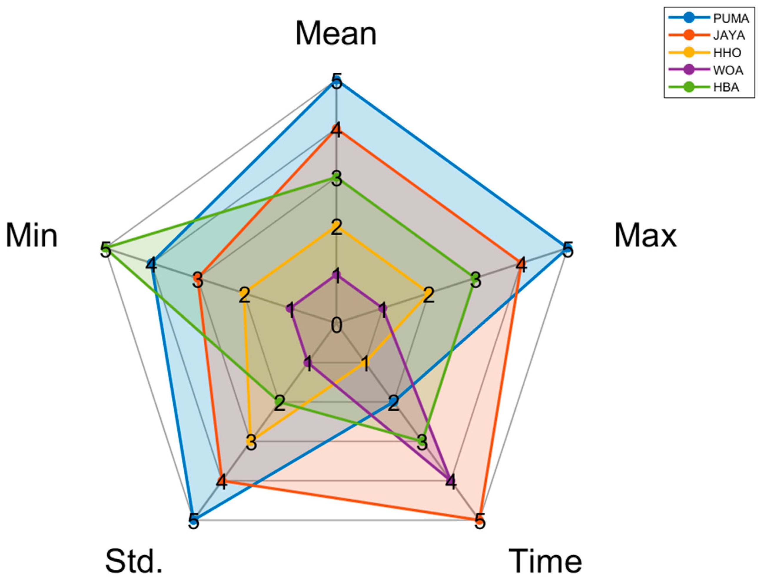
• Integrate the algorithm performance variables into a visual analysis using radar charts.
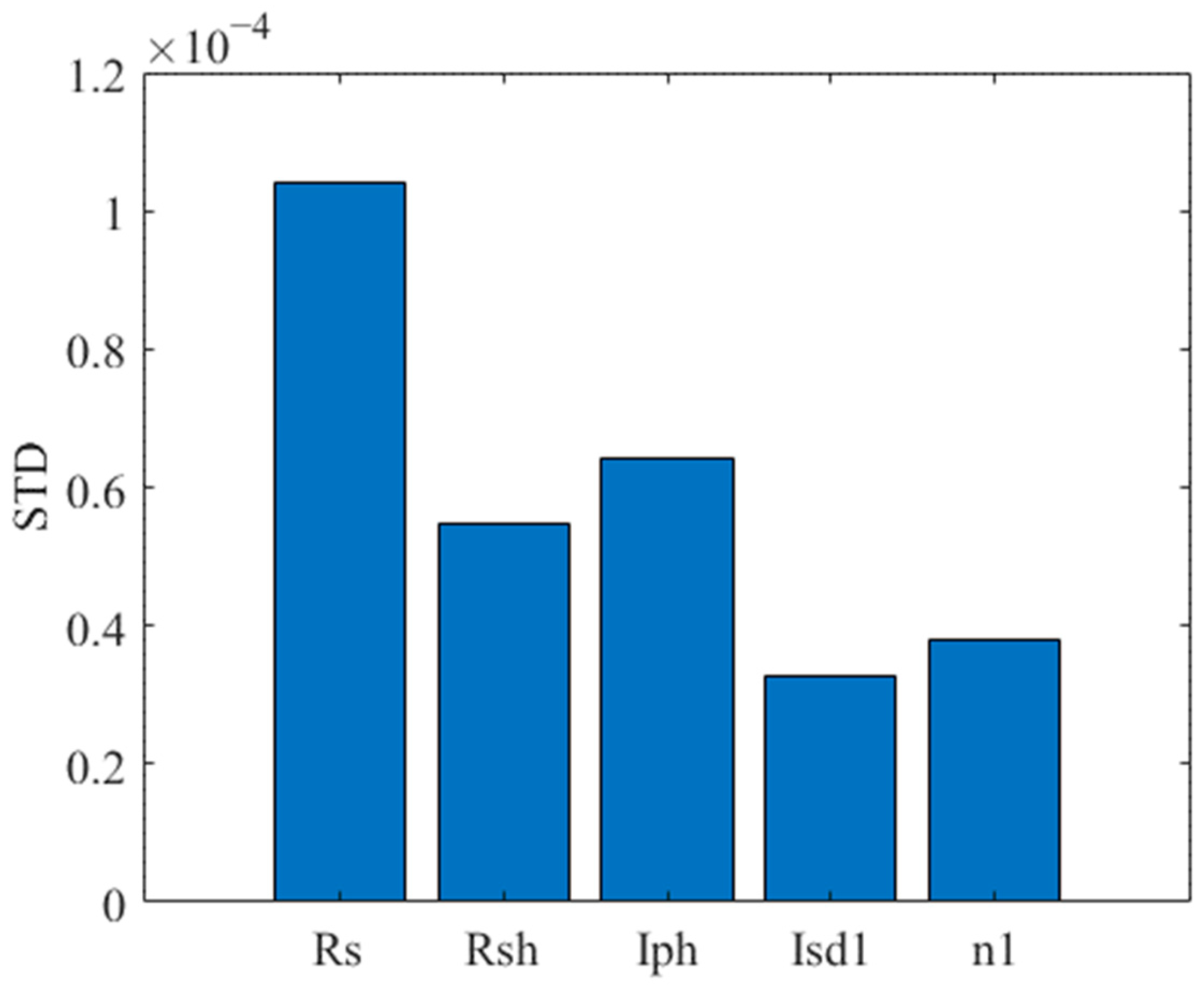
• Use a one-factor-at-a-time approach to analyze the sensitivity of system parameters.

2. Methodology

2.1. Photovoltaics Modeling

To efficiently characterize the behavior of PV models, it is necessary to establish an appropriate mathematical model. For all intents and purposes, PV systems can be considered to be fundamentally similar to photodiodes. In this study, four PV circuit models are explored in depth: SDM, DDM, TDM, and PMM. The following section will elaborate on the mathematical description of these models and introduce the uncertainty parameters used for parameter identification.

2.1.1. Single Diode Model

SDM is the simplest model, and it considers the effects of negative impurities, defects and leakage current that might exist in the PV system. The terminal current I_L is shown in Equation (1), where I_ph is the photocurrent source; R_S is the series resistor; and R_sh is the shunt resistor [51].

$$I_L=I_{ph}-I_D-I_{sh}$$

(1)

$$I_D=I_{sd1}\left[\exp \left({\displaystyle \frac{q\left(V_L+I_L{R}_S\right)}{n_{1}kT}}\right)-1\right]$$

(2)

$$I_{sh}={\displaystyle \frac{V_L+I_L{R}_S}{R_{sh}}}$$

(3)

Equation (2) shows the calculation for the diode current I_D according to the Shockley diode equation, where I_sd1 is the reverse saturation current of the diode; V_L is the terminal voltage; n₁ is the ideality factor of the diode (of which the ideality factor of silicon PV cells is between 1 and 2); k is the Boltzmann constant ($1.6\times {10}^{-23}$ J/K); q is the electron charge ($1.608\times {10}^{-19}$ C); and T is the absolute temperature of the battery in Kelvin. Equation (3) presents the calculation for the current of the shunt resistor I_sh; R_sh is the parallel resistance which represents the leakage current generated in the PV cell, and the SDM parameters are [$I_{ph}, I_{sd1}, R_s,R_{sh},n_1$]. The equivalent circuit diagram of the SDM is shown in Figure 2.

2.1.2. Double Diode Model

As compared to SDM, DDM includes an additional parallel diode to account for combination current loss, which becomes increasingly significant under low irradiance conditions. While being more complex than SDM, DDM provides greater accuracy. The calculation of the DDM terminal current is shown in Equation (4) [52].

$$I_L=I_{ph}-I_{D_1}-I_{D_2}-I_{sh}$$

(4)

The calculation for I_sh was previously shown in Equation (3), while the calculations of I_D1 and I_D2 are expressed in Equations (5) and (6) below.

$$I_{D_1}=I_{sd1}\left[\exp \left({\displaystyle \frac{q\left(V_L+I_L{R}_S\right)}{n_{1}kT}}\right)-1\right]$$

(5)

$$I_{D_2}=I_{sd2}\left[\exp \left({\displaystyle \frac{q\left(V_L+I_L{R}_S\right)}{n_{2}kT}}\right)-1\right]$$

(6)

In Equations (5) and (6) above, I_sd1 and I_sd2 represent the reverse saturation current generated by the diffusion and recombination phenomena, respectively; n₁ and n₂ are the diffusion and recombination ideality factors of the diode, respectively; I_sh was previously calculated in Equation (3); and the parameters to be identified in the DDM are [$I_{ph},I_{sd1},I_{sd2},R_s,R_{sh},n_1,n_2$]. The equivalent circuit diagram is shown in Figure 3.

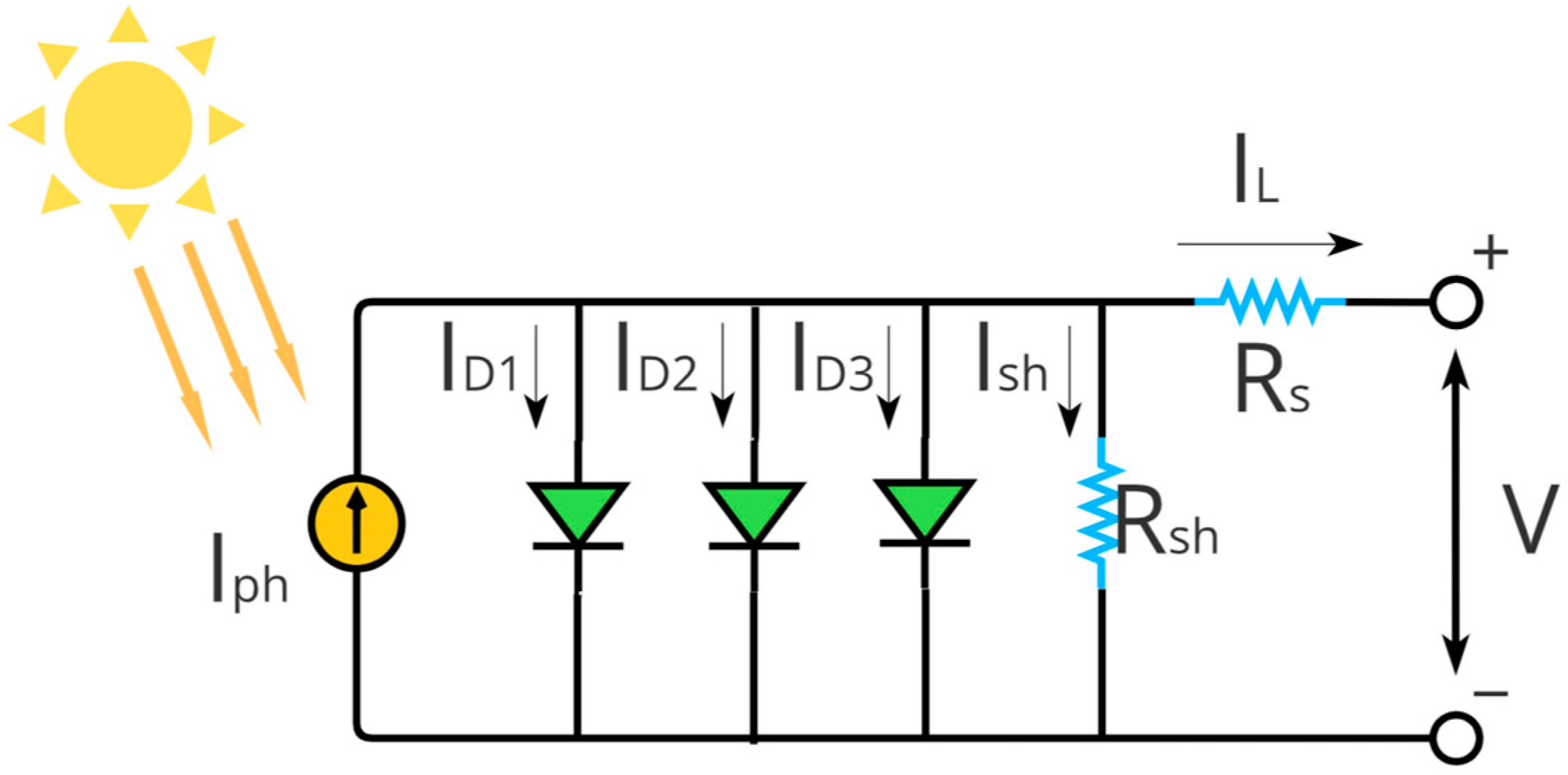
2.1.3. Triple Diode Model

Building upon the previous model, TDM further accounts for leakage current generated by recombination at grain and surface boundaries, and thus offers a more accurate representation of the losses caused by potential defects and non-ideal conditions in PV cells. The equivalent circuit diagram of the TDM is shown in Figure 4, and the calculation for the terminal voltage I_L is shown in Equation (7) below [53].

$$I_L=I_{ph}-I_{D_1}-I_{D_2}-I_{D_3}-I_{sh}$$

(7)

The calculation for I_sh was previously shown in Equation (3), while the calculations for I_D1, I_D2 and I_D3 are expressed below in Equations (8), (9) and (10), respectively.

$$I_{D_1}=I_{sd1}\left[\exp \left({\displaystyle \frac{q\left(V_L+I_L{R}_S\right)}{n_{1}kT}}\right)-1\right]$$

(8)

$$I_{D_2}=I_{sd2}\left[\exp \left({\displaystyle \frac{q\left(V_L+I_L{R}_S\right)}{n_{2}kT}}\right)-1\right]$$

(9)

$$I_{D_3}=I_{sd3}\left[\exp \left({\displaystyle \frac{q\left(V_L+I_L{R}_S\right)}{n_{3}kT}}\right)-1\right]$$

(10)

In the equations above, I_sd3 represents the reverse saturation current generated by the grain boundary effect; n₃ is the ideality factor of the third diode; and the parameters to be identified in the TDM are [$I_{ph}$, $I_{sd1}$, $I_{sd2}$, $I_{sd3}$, $R_s$, $R_{sh}$, $n_1$, $n_2$, $n_3$].

2.1.4. Photovoltaic Module Model

PMM extends the single diode model to represent the behavior of interconnected PV cells within a module. As shown in Figure 5, the model incorporates series ($N_s$) and parallel ($N_p$) cell configurations to account for practical module construction. The output current is divided by the number of parallel-connected cells $N_p$ and the terminal voltage is normalized by the number of series connected cells $N_s$ [54].

$$I_L=N_p(I_{ph}-I_D-I_{sh})$$

(11)

$$I_D=I_{sd1}\left[\exp \left({\displaystyle \frac{q\left(V_L/N_s+I_L{R}_S/N_p\right)}{n_{1}kT}}\right)-1\right]$$

(12)

$$I_{sh}={\displaystyle \frac{V_L/N_s+I_L{R}_S/N_p}{R_{sh}}}$$

(13)

2.2. Puma Optimizer

Puma Optimizer (PO) was proposed by Abdollahzadeh et al. and is a swarm intelligence (SI) algorithm inspired by the behavior and hunting habits of pumas [55]. The algorithm features a powerful search mechanism that maintains a balance between exploration and exploitation. The PO is capable of executing phase transitions during the optimization process and can dynamically switch between different search phases. This section is going to introduce the mathematical model of the algorithm.

2.2.1. Initialization

First of all, pumas are randomly initialized within the search area.

$$\mathrm{A}=\left[\begin{array}{c}{x}_1\\ x_2\\ \dots \\ x_n\end{array}\right]=\left[\begin{array}{cc}\begin{array}{cc}{x}_{11}& x_{12}\\ x_{21}& x_{22}\end{array}& \begin{array}{ccc}{x}_{13}& \dots & x_{1D}\\ x_{23}& \dots & x_{2D}\end{array}\\ \begin{array}{cc} & \dots \\ x_{n1}& x_{n2}\end{array}& \begin{array}{ccc}\dots & \dots & \\ x_{n3}& \dots & x_{nD}\end{array}\end{array}\right]$$

(14)

In Equation (14), A represents the total population of pumas; X_i represents the position of the ith puma; n represents the number of pumas; and D represents the dimension of the problem.

$${\mathrm{x}}_{\mathrm{i}}=L{B}_{\mathrm{i}}+{\mathrm{r}}_1\ast \left(U{B}_{\mathrm{i}}-L{B}_{\mathrm{i}}\right)$$

(15)

In Equation (15), the pumas’ positions are generated between the upper bound (UB) and lower bound (LB), where r₁ represents a random number between [0, 1] and x_i represents the position of the ith puma.

2.2.2. Inexperienced Phase

In the initial phase of the algorithm, pumas are still inexperienced. Accordingly, in the first three iterations of PO, both exploration and exploitation phases are executed simultaneously. n represents number of pumas in a group. The original puma population A will generate two new populations in each iteration, with the new populations represented as A_explore and A_exploit. The population set comprising the three groups is expressed as A_pop = [A A_explore A_exploit]. The set A_pop is then evaluated and sorted by fitness, retaining the top-performing pumas at the end of each iteration to ensure optimal evolutionary direction. After the first three iterations, functions f1 and f2 are calculated to assess the performance of the exploration and exploitation phases, with the corresponding scores represented as Score_Explore and Score_Exploit, respectively. These scores then serve as indicators to determine the search phase to be implemented during the experienced phase. The algorithm executes the steps as follows:

Equations (16)–(19): Calculation of f1 and f2.

Equations (20)–(25): Calculation of the variable Seq found in f1 and f2.

Equations (26) and (27): Calculation of the final scores of the exploration and exploitation phases, namely Score_Explore and Score_Exploit.

$$f{1}_{Explore}=P{F}_1·\left({\displaystyle \frac{Se{q}_{Cost Explore}^1}{Se{q}_{Time}}}\right)$$

(16)

$$f{1}_{Exploit}=P{F}_1·\left({\displaystyle \frac{Se{q}_{Cost Exploit}^1}{Se{q}_{Time}}}\right)$$

(17)

$$f{2}_{Explore}=P{F}_2·\left({\displaystyle \frac{Se{q}_{Cost Explore}^1+Se{q}_{Cost Explore}^2+Se{q}_{Cost Explore}^3}{Se{q}_{Time}^1+Se{q}_{Time}^2+Se{q}_{Time}^3}}\right)$$

(18)

$$f{2}_{Exploit}=P{F}_2·\left({\displaystyle \frac{Se{q}_{Cost Exploit}^1+Se{q}_{Cost Exploit}^2+Se{q}_{Cost Exploit}^3}{Se{q}_{Time}^1+Se{q}_{Time}^2+Se{q}_{Time}^3}}\right)$$

(19)

In Equations (16)–(19), f1_Explore and f2_Explore represent the calculations of f1 and f2 for the exploration search, f2_Exploit and f1_Exploit represent the calculations of f1 and f2 for the exploitation search. The variables $Se{q}_{\mathrm{Cost}Explore}^t$ and $Se{q}_{Cost Exploit}^t$ represent the calculation results of Seq during the exploration and exploitation search at the t^th iteration. In Equations (20)–(25), $Se{q}_{\mathrm{Time}}^t$ represents the number of times each phase was chosen. Because both searches are selected in every iteration during the inexperienced phase, the value of $Se{q}_{\mathrm{Time}}^t$ will be 1. Lastly, PF₁ and PF₂ represent the priority factors of f1 and f2 which are used to determine the relative priority between the two functions. The initial values of PF₁ and PF₂ are set to 0.5.

$$Se{q}_{Cost Explore}^1=\left|{Cost}_{Best}^{Initial}-{Cost}_{Explore}^1\right|$$

(20)

$$Se{q}_{Cost Explore}^2=\left|{Cost}_{Explore}^2-{Cost}_{Explore}^1\right|$$

(21)

$$Se{q}_{Cost Explore}^3=\left|{Cost}_{Explore}^3-{Cost}_{Explore}^2\right|$$

(22)

$$Se{q}_{Cost Exploit}^1=\left|{Cost}_{Best}^{Initial}-{Cost}_{Exploit}^1\right|$$

(23)

$$Se{q}_{Cost Exploit}^2=\left|{Cost}_{Exploit}^2-{Cost}_{Exploit}^1\right|$$

(24)

$$Se{q}_{Cost Exploit}^3=\left|{Cost}_{Exploit}^3-{Cost}_{Exploit}^2\right|$$

(25)

In Equations (20)–(25) above, ${Cost}_{Best}^{Initial}$ represents the best fitness value in the previous population, while ${Cost}_{Explore}^t$ and ${Cost}_{Exploit}^t$ represent the best fitness values in the puma populations A_explore and A_exploit generated in the exploration and exploitation phases at the tth iteration, respectively. f1 and f2 represent the mean differences in the best fitness values across the different phases and iterations.

$$Scor{e}_{Explore}=\left(P{F}_1·f{1}_{Explore}\right)+\left(P{F}_2·f{2}_{Explore}\right)$$

(26)

$$Scor{e}_{Exploit}=\left(P{F}_1·f{1}_{Exploit}\right)+\left(P{F}_2·f{2}_{Exploit}\right)$$

(27)

In Equations (26) and (27) above, PF₁ and PF₂ are constants set to 0.5. f1_Explore, f2_Explore, f1_Exploit and f2_Exploit represent the values obtained from the exploration and exploitation calculations. If Score_Explore is greater than Score_Exploit, the phase selected in the following experienced phase will be exploration. Conversely, if Score_Exploit is greater than Score_Explore, the phase will instead be exploitation.

2.2.3. Experienced Phase

After completing the first three iterations during the inexperienced phase, the puma will choose one search mechanism to execute based on the accrued experience. Thereafter, it will continue to change search strategy between iterations. The algorithm will select explore or exploitation according to values f1, f2 and f3. These functions serve to integrate the established effectiveness of exploration and exploitation operations, ensuring that the most advantageous phase will be chosen for successive iterations. The calculation methods for f1, f2 and f3 for this phase are elaborated below. These methods allow the algorithm to effectively evaluate and transition between search mechanisms, thereby enhancing its global and local search capabilities.

The calculation method for f1 is shown in Equations (28) and (29) below.

$${f_1}_t^{exploit}=P{F}_1·\left|{\displaystyle \frac{Cos{t}_{old}^{exploit}-Cos{t}_{new}^{exploit}}{T_t^{exploit}}}\right|$$

(28)

$${f_1}_t^{explore}=P{F}_1·\left|{\displaystyle \frac{Cos{t}_{old}^{explore}-Cos{t}_{new}^{explore}}{T_t^{explore}}}\right|$$

(29)

${f_1}_t^{exploit}$ represents the calculation method of f1 in the exploitation phase; ${f_1}_t^{explore}$ represents the calculation method of f1 in the exploration phase; t represents the current iteration number; PF₁ represent the priority factor for f1 and needs to be set to a value between [0, 1] at the start of the algorithm; $Cos{t}_{old}^{exploit}$ and $Cos{t}_{old}^{explore}$ represent the old best fitness values for the pumas in the population; $Cos{t}_{new}^{exploit}$ and $Cos{t}_{new}^{explore}$ represent the new best fitness values for the population after each phase is executed; while $T_t^{exploit}$and $T_t^{explore}$ represent the number of iterations that the phases have been unselected for since they were last chosen.

The calculation method for f2 is shown in Equations (30) and (31) below.

$${f_2}_t^{exploit}=P{F}_2·\left|{\displaystyle \frac{S_1^{exploit}+S_2^{exploit}+S_3^{exploit}}{T_{t,1}^{exploit}+T_{t,2}^{exploit}+T_{t,3}^{exploit}}}\right|$$

(30)

$${f_2}_t^{explore}=P{F}_2·\left|{\displaystyle \frac{S_1^{explore}+S_2^{explore}+S_3^{explore}}{T_{t,1}^{explore}+T_{t,2}^{explore}+T_{t,3}^{explore}}}\right|$$

(31)

${f_2}_t^{exploit}$ and ${f_2}_t^{explore}$ represents the calculation method of f2 in the exploitation and exploration phases, respectively. t represents the current iteration number, and PF₂ represents the priority factor for f2 and needs to be set to a value between [0, 1] at the start of the algorithm.

$$S_1^{exploit}=Cos{t}_{Old,1}^{exploit}-Cos{t}_{New,1}^{exploit}$$

(32)

$$S_2^{exploit}=Cos{t}_{Old,2}^{exploit}-Cos{t}_{New,2}^{exploit}$$

(33)

$$S_3^{exploit}=Cos{t}_{Old,3}^{exploit}-Cos{t}_{New,3}^{exploit}$$

(34)

$$S_1^{explore}=Cos{t}_{Old,1}^{explore}-Cos{t}_{New,1}^{explore}$$

(35)

$$S_2^{explore}=Cos{t}_{Old,2}^{explore}-Cos{t}_{New,2}^{explore}$$

(36)

$$S_3^{explore}=Cos{t}_{Old,3}^{explore}-Cos{t}_{New,3}^{explore}$$

(37)

In Equations (32)–(27), S^exploit and S^explore represent the cost difference between the two phases. $Cos{t}_{Old}^{exploit}$ and $Cos{t}_{Old}^{explore}$ represent t old best fitness values of the solution in the current exploitation and exploration phase selections. $Cos{t}_{New}^{exploit}$ and $Cos{t}_{New}^{explore}$ represent the new best fitness values of the solution in the current exploitation and exploration phase selections. $T_t^{explore}$and $T_t^{exploit}$ represent the number of iterations that the exploration and exploitation phases have been unselected for since they were last chosen.

The calculation method for f3 is shown in Equations (38) and (39) below.

$${f_3}_t^{exploit}=\left\{\begin{array}{c}if selected, {f_3}_t^{exploit}=0\\ otherwise, {f_3}_t^{exploit}+P{F}_3\end{array}\right.$$

(38)

$${f_3}_t^{explore}=\left\{\begin{array}{c}if selected, {f_3}_t^{explore}=0\\ otherwise, {f_3}_t^{explore}+P{F}_3\end{array}\right.$$

(39)

In Equations (38) and (39), ${f_3}_t^{exploit}$ and ${f_3}_t^{explore}$represent the calculation expressions of f3 in the exploitation and exploration phases. t represents the current iteration number and PF₃ is a constant value of 0.3 in the algorithm.

Equations (40) and (41) below show the score calculation expressions for the exploration and exploitation phases.

$$F_t^{explore}=\left({\alpha }_t^{explore}·\left({f_1}_t^{explore}\right)\right)+\left({\alpha }_t^{explore}·\left({f_2}_t^{explore}\right)\right)+\left({\delta }_t^{explore}·\left(lc·{f_3}_t^{explore}\right)\right)$$

(40)

$$F_t^{exploit}=\left({\alpha }_t^{exploit}·\left({f_1}_t^{exploit}\right)\right)+\left({\alpha }_t^{exploit}·\left({f_2}_t^{exploit}\right)\right)+\left({\delta }_t^{exploit}·\left(lc·{f_3}_t^{exploit}\right)\right)$$

(41)

In the above equation, $F_t^{explore}$ and $F_t^{exploit}$ represent the scores of the exploration and exploitation phase in the current iteration, while lc, α and δ are defined in Equations (42)–(45) below.

$$lc=\left\{\begin{array}{c}{\left\{\left|Cos{t}_{old}-Cos{t}_{New}\right|\right\}}^{exploitation}\\ {\left\{\left|Cos{t}_{old}-Cos{t}_{New}\right|\right\}}^{exploration}\end{array}\right\}, 0\notin lc$$

(42)

$$\begin{array}{c}{\alpha }_t^{explore, exploit}=\\ if F^{exploit}>F^{explore}:{\alpha }^{exploit}=0.99,{\alpha }^{explore}=\lceil {\alpha }^{explore}-0.01,0.01\rceil \\ otherwise:{\alpha }^{explore}=0.99,{\alpha }^{exploit}=\lceil {\alpha }^{exploit}-0.01,0.01\rceil \end{array}$$

(43)

$${\delta }_t^{exploit}=1-{\alpha }_t^{exploit}$$

(44)

$${\delta }_t^{explore}=1-{\alpha }^{explore}$$

(45)

In Equation (42), lc represents the calculation of the difference in best fitness values of the exploration and exploitation phase before and after the iteration. In Equation (43), α^explore and α^exploit respectively represent the values of α in the exploration and exploitation phase, while F^explore and F^exploit respectively represent the scores of the previous exploration and exploitation phases. Lastly, in Equations (44) and (45), ${\delta }_t^{exploit}$ and ${\delta }_t^{explore}$ represent the values of δ in the exploitation and exploration phases, respectively. The algorithm intelligently adjusts the weightage of f1 and f2 based on the scores of the exploration and exploitation phases. When the score of the exploitation phase is greater than that of the exploration phase, it indicates that the weight of exploitation is too low, and the weight of exploration will be linearly reduced through α. Conversely, if the score of the exploration is greater than that of exploitation, the opposite adjustment is implemented. By switching between different phases through the continuous score calculations for exploration and exploitation, the algorithm effectively prevents premature convergence to local optima and avoids excessive global searches which could lead to inaccurate solutions.

2.2.4. Exploration Phase

This phase imitates pumas’ prey-searching behavior, where they travel to new areas or randomly approach other pumas during the exploration process. The position of the puma is updated according to Equation (46) to improve the search efficiency and expand the exploration range. If rand₁ is greater than 0.5, then execute Equation (46); otherwise, Equation (47) is applied.

$$Z_{i,G}=R_{Dim}\times \left(UB-LB\right)+LB$$

(46)

$$Z_{i,G}=X_{a,G}+G·\left(X_{a,G}-X_{b,G}\right)+G·\left(\left(\left(X_{a,G}-X_{b,G}\right)-\left(X_{c,G}-X_{d,G}\right)\right)+\left(\left(X_{c,G}-X_{d,G}\right)-\left(X_{e,G}-X_{f,G}\right)\right)\right)$$

(47)

$$G=2·ran{d}_2-1$$

(48)

In Equations (46) and (47), UB and LB represent the upper and lower search boundaries and X_a,G, X_b,G, X_c,G, X_d,G, X_e,G, X_f,G represent the solutions of six random pumas from the population. In Equation (48), rand₂ is a random number between [0, 1] and G falls between [−1, 1] and can be considered as a directional factor. Equations (49)–(52) below determined the replacement strategy for deciding whether the new solution should replace the old one.

$$X_{new}=\left\{\begin{array}{c}{Z}_{i,G}, if j=j_{rand} or ran{d}_3\le U\\ X_{a,G}, otherwise\end{array}\right.$$

(49)

$$NC=1-U$$

(50)

$$p={\displaystyle \frac{NC}{Npop}}$$

(51)

$$\begin{gathered} if Cost{X}_{new}<Cost{X}_i:X_{a,G}=X_{new} \\ \mathit{Otherwise}:U=U+p \end{gathered}$$

(52)

In Equation (49), Z_i,G represents the i-th puma solution generated in Equations (46) and (47); j_rand is a randomly generated integer in the dimensional range; rand₃ is a random number between [0, 1]; and U is a decreasing value between [0, 1], with an initial preset value of 0.2. N_pop represents the total number of the puma population; and U is a value that constantly increases through the value of p, where the p is calculated in Equation (51). In Equation (52), CostX_new represents the fitness value of the new solution; CostX_i represents the fitness value of the original solution.

2.2.5. Exploitation Phase

As inspired by the hunting habits of the puma, the algorithm uses two different search mechanisms to obtain new solutions by ambush and sprinting strategy. The mathematical models of these mechanisms are elaborated upon in Equations (53)–(59) below.

$$\begin{gathered} {rand}_4\ge 0.5:X_{new}={\displaystyle \frac{\left(\frac{mean\left(So{l}_{total}\right)}{Npop}\right)·X_1^r-{\left(-1\right)}^{\beta }\times X_i}{1+\left(\alpha ·ran{d}_5\right)}} \\ \text{otherwise}: \\ {rand}_6\ge L:X_{new}=Pum{a}_{male}+\left(2·ran{d}_7\right)·exp\left(rand{n}_1\right)·\left(X_2^r-X_i\right) \\ \mathrm{otherwise}:X_{new}=\left(2\times ran{d}_8\right)\times {\displaystyle \frac{\left(F_1·R·X\left(i\right)+F2·\left(1-R\right)·Pum{a}_{male}\right)}{\left(2·ran{d}_9-1+rand{n}_2\right)}}-Pum{a}_{male} \end{gathered}$$

(53)

$$X_2^r=round\left(1+\left(Npop-1\right)· ran{d}_{10}\right)$$

(54)

$$R=2·ran{d}_{11}-1$$

(55)

$$F_1=rand{n}_3·exp\left(2-Iter·\left({\displaystyle \frac{2}{MaxIter}}\right)\right)$$

(56)

$$F_2=w\times {\left(v\right)}^2·cos\left(\left(2\times ran{d}_{12}\right)·w\right)$$

(57)

$$w=rand{n}_4$$

(58)

$$v=rand{n}_5$$

(59)

In the Equations above, rand is a random number between [0, 1], and if rand₄ ≥ 0.5, the sprinting strategy is executed; otherwise, the ambush strategy is applied. And if rand₆ ≥ L, where L represents a constant set to 0.67, short jumps are performed; otherwise, long jumps are performed. $mean\left(So{l}_{total}\right)$ represents the average of all solutions in the population; N_pop represents the total puma population; $X_1^r$ represents a solution randomly selected from the entire population; Puma_male represents the best individual in the population; β is a constant randomly set to either 0 or 1; α is a constant set to 2; exp represents the exponential function, randn₁ and randn₂ represent random numbers following normal distribution; and $X_2^r$ is a solution randomly selected according to Equation (54).

Following that, R, F1, and F2 are calculated using Equations (55)–(57), where randn₃ represents a random number following normal distribution; exp represents the exponential function; Iter represents the current iteration number; and MaxIter represents the maximum number of iterations. In Equation (56), cos represents the cosine function. In Equations (58) and (59), parameters w and v are defined as rand_n4 and rand_n5 which represent random numbers following normal distribution. At the end of the exploitation phase, the superior individuals are retained after comparing the fitness values of the new and old solutions. The algorithm flowchart is shown below as Figure 6.

2.3. Objective Function

During the process of parameter identification, the algorithm continuously searches for model parameters within the search space until the set number of iterations is reached. The algorithm aims to obtain search optimal parameter solutions that can approach experimental data. This study uses the root mean square error (RMSE) as the objective function to calculate the error between the calculated and experimental current, which is shown in Equation (60) below.

$$RMSE=\sqrt{{\displaystyle \frac{1}{N}}{\displaystyle \sum }_{t=1}^N{\left(I_{caculated}-I_{experimental}\right)}^2}=\sqrt{{\displaystyle \frac{1}{N}}{\displaystyle \sum }_{t=1}^N{\left(f_{model}\left(V_L,I_L,x\right)-I_t\right)}^2}$$

(60)

Here, N represents the number of data points; I_caculated represents the value of the calculated current; I_experimental represents the value of the experimental current; V_L and I_L represent the experimental terminal voltage and experimental terminal current, respectively; x represents the parameter array, which is defined in Table 1; and f represents the objective functions of the three models. The PV model’s unscented parameters are shown in

Table 2. The photovoltaic model parameter array.

Function	Parameter Vector
$f_{SDM}$	$x=[I_{ph}$$,I_{sd1}$$,R_s$$,R_{sh}$$,n_1$]
$f_{DDM}$	$x=[I_{ph}$$,I_{sd1}$$,I_{sd2}$$,R_s$$,R_{sh}$$,n_1$$,n_2$]
$f_{TDM}$	$x=[I_{ph}$$,I_{sd1}$$,I_{sd2}$$,I_{sd3}$$,R_s$$,R_{sh}$$,n_1$$,n_2$$,n_3$]
$f_{PMM}$	$x=[I_{ph}$$,I_{sd1}$$,R_s$$,R_{sh}$$,n_1$]

.

The parameter sensitivity function is calculated as shown in Equation (61). We use the one-factor-at-a-time method to determine the importance level of each parameter in the PV model.

$$STD=\sqrt{{\displaystyle \frac{1}{N}}{\displaystyle \sum }_{Z=0.8}^{1.2}{\left(RMS{E}_z-\overline{RMSE}\right)}^2}$$

(61)

In this approach, STD represents the standard deviation of the results across different values of a given parameter. N represents the number of data points. RMSE_z denotes the root mean square error corresponding to each variation in the parameter. The parameter values are varied over a range from 0.8 to 1.2 times their nominal values denoted as z. $\overline{RMSE}$ is the average error across all cases.

2.4. Parameter Setting

To verify the suitability of PO for PV parameter identification and to boost further performance prediction, this study made use of a widely adopted PV dataset from the commercial R.T.C France solar cell and solar module Photowatt-PWP 201 [56]. The relevant cell and module specifications, along with the parameter search ranges, are provided in

Table 3. Specifications of commercial PV cell [57].

57 mm Diameter R.T.C France Solar Cell
Operation Temperature (K)	303.15
Operation radiation (W/m2)	1000
Maximum power (Pmpp) (W)	0.3101
Voltage at MPP (VMPP) (V)	0.4507
Current at MPP (IMPP) (A)	0.6880
Open circuit voltage (VOC) (V)	0.5728
Short circuit current (ISC) (A)	0.7603

,

Table 4. Photovoltaic cell parameter identification range.

	Parameter	Range		Parameter	Range
1	Iph (A)	[0, 1]	6	Isd2 (μA)	[0.001, 1]
1	Rs (Ω)	[0, 0.5]	7	n2	[1, 2]
2	Rsh (Ω)	[0, 100]	8	Isd3 (μA)	[0.001, 1]
4	Isd1 (μA)	[0.001, 1]	9	n3	[1, 2]
5	n1	[1, 2]	-	-	-

,

Table 5. Specifications of commercial PV module [58].

Photowatt-PWP 201 Solar Module
Operation Temperature (K)	318.15
Operation radiation (W/m2)	1000
Maximum power (Pmpp) (W)	11.54
Voltage at MPP (VMPP) (V)	12.6490
Current at MPP (IMPP) (A)	0.9120
Open circuit voltage (VOC) (V)	16.7785
Short circuit current (ISC) (A)	1.0317

and

Table 6. Photovoltaic module parameter identification range.

	Parameter	Range		Parameter	Range
1	Iph (A)	[0, 2]	4	Isd1 (μA)	[0, 50]
2	Rs (Ω)	[0, 2]	5	n1	[1, 50]
3	Rsh (Ω)	[0, 2000]

.

To assess the robustness of PO algorithm, we compared four additional metaheuristic algorithms: whale optimization algorithm, honey badger algorithm, Harris Hawks optimization and JAYA Algorithm. The parameter settings for each algorithm are listed in

Table 7. The optimization algorithm setting.

Algorithm Setting
Independent run time	30
Population size	30
Iteration time	1000

. The research was conducted using equipment featuring an 11th Gen Intel Core i5-11320H CPU, manufactured by Intel Corporation (Santa Clara, CA, USA) and MATLAB R2022b.

3. Results and Discussion

PO and the four other algorithms were applied to identify parameters of three PV models (SDM, DDM, TDM and PMM), the calculation results of which will be discussed in detail in the following section. To evaluate the calculation process and suitability of each algorithm in depth, the study will calculate the best fitness, mean fitness, and standard deviation (Std.) of the algorithms and perform statistical analysis on their performances through the methods of convergence history, error bar and boxplot.

3.1. Single Diode Model

For the SDM parameter identification, five algorithms were used to identify five undetermined parameters.

Table 8. SDM experimental data compared against five advanced algorithms.

Experimental Data		HBA	WOA	HHO	JAYA	PO
Vt(V)	It(A)	Computed It(A)
−0.2057	0.7640	0.7642	0.7632	0.7637	0.7629	0.7642
−0.1291	0.7620	0.7628	0.7620	0.7623	0.7618	0.7628
−0.0588	0.7605	0.7614	0.7609	0.7611	0.7607	0.7614
0.0057	0.7605	0.7602	0.7600	0.7600	0.7598	0.7602
0.0646	0.7600	0.7590	0.7591	0.7590	0.7589	0.7590
0.1185	0.7590	0.7580	0.7582	0.7581	0.7581	0.7580
0.1678	0.7570	0.7570	0.7574	0.7572	0.7573	0.7570
0.2132	0.7570	0.7560	0.7566	0.7563	0.7565	0.7560
0.2545	0.7555	0.7550	0.7557	0.7553	0.7556	0.7550
0.2924	0.7540	0.7535	0.7543	0.7540	0.7542	0.7535
0.3269	0.7505	0.7513	0.7520	0.7517	0.7519	0.7513
0.3585	0.7465	0.7473	0.7478	0.7476	0.7478	0.7473
0.3873	0.7385	0.7401	0.7404	0.7403	0.7403	0.7401
0.4137	0.7280	0.7275	0.7273	0.7275	0.7273	0.7275
0.4373	0.7065	0.7071	0.7066	0.7069	0.7065	0.7071
0.4590	0.6755	0.6755	0.6747	0.6750	0.6745	0.6755
0.4784	0.6320	0.6309	0.6301	0.6303	0.6298	0.6309
0.4960	0.5730	0.5720	0.5715	0.5714	0.5710	0.5720
0.5119	0.4990	0.4995	0.4996	0.4990	0.4990	0.4995
0.5265	0.4130	0.4134	0.4143	0.4132	0.4135	0.4134
0.5398	0.3165	0.3171	0.3187	0.3172	0.3179	0.3171
0.5521	0.2120	0.2118	0.2137	0.2121	0.2131	0.2118
0.5633	0.1035	0.1022	0.1038	0.1026	0.1036	0.1022
0.5736	−0.0100	−0.0083	−0.0079	−0.0080	−0.0073	−0.0083
0.5833	−0.1230	−0.1243	−0.1257	−0.1243	−0.1242	−0.1243
0.5900	−0.2100	−0.2065	−0.2101	−0.2070	−0.2077	−0.2065
RMSE		$8.8186\times {10}^{-4}$	$1.2986\times {10}^{-3}$	$9.4210\times {10}^{-4}$	$1.1566\times {10}^{-3}$	$8.8180\times {10}^{-4}$

presents the comparison between the experimental current and the computed current obtained by each algorithm.

Table 9. The results of the SDM parameter identification.

PARAM/ALGO	OBEDO [37]	$\mathit{\mu }$AFCSO [58]	ESMA [30]	HBA	WOA	HHO	JAYA	PO
Rs (Ω)	0.0364	0.03639	0.036373	0.037	0.0349	0.0363	0.0354	0.037
$R_{sh}$ (Ω)	53.7185	52.64088	53.724744	51.8812	65.4335	58.5555	67.1110	52.1089
$I_{ph}$ (A)	0.7608	0.76091	0.760776	0.7608	0.7605	0.7606	0.7602	0.7608
$I_{sd1}$ (μA)	${3.2310}^{-7}$	0.32168	0.323260	0.2905	0.4395	0.3476	0.4258	0.2918
n1	1.4812	1.48077	1.481095	1.4719	1.5142	1.4899	1.5109	1.4723
Best	$9.8602\times {10}^{-4}$ (5)	$9.8314\times {10}^{-4}$ (4)	$9.860231\times {10}^{-4}$ (6)	$8.8186\times {10}^{-4}$ (2)	$1.2986\times {10}^{-3}$ (8)	$9.4210\times {10}^{-4}$ (3)	$1.1566\times {10}^{-3}$ (7)	$8.8180\times {10}^{-4}$ (1)
Mean	$9.8602\times {10}^{-4}$ (3)	$9.8314\times {10}^{-4}$ (2)	$1.499893\times {10}^{-3}$ (5)	$6.3622\times {10}^{-3}$ (6)	$1.2364\times {10}^{-2}$ (8)	$7.0523\times {10}^{-3}$ (7)	$1.4668\times {10}^{-3}$ (4)	$9.3341\times {10}^{-4}$ (1)
Std.	$4.7451\times {10}^{-17}$ (1)	$2.4921\times {10}^{-14}$ (2)	$4.828118\times {10}^{-4}$ (5)	$1.3270\times {10}^{-2}$ (7)	$1.5128\times {10}^{-2}$ (8)	$8.1770\times {10}^{-3}$ (6)	$1.6326\times {10}^{-4}$ (4)	$8.3827\times {10}^{-5}$ (3)

shows the values of the optimal parameters, best fitness, mean fitness and standard deviation of 30 independent operations executed by each algorithm. Figure 7 displays the mean and best convergence curves of the algorithms. The results show that PO was also significantly faster than all the other algorithms during the iterative process. The analytical methods are illustrated in Figure 8. PO also shows a significant advantage in computational stability. Figure 9 plots the I–V and P–V curves based on PO results in comparison with the experimental values. Figure 10 shows the prediction of the characteristic curves under four temperature conditions (25, 33, 50 and 75 °C), with the MPPs at different temperatures marked by black dots.

3.2. Double Diode Model

For the DDM parameter identification, the algorithms were used to identify seven undetermined parameters.

Table 10. DDM experimental data compared against five advanced algorithms.

Experimental Data		HBA	WOA	HHO	JAYA	PO
Vt(V)	It(A)	Computed It(A)
−0.2057	0.7640	0.7641	0.7662	0.7611	0.7636	0.7641
−0.1291	0.7620	0.7627	0.7645	0.7603	0.7624	0.7627
−0.0588	0.7605	0.7614	0.7630	0.7595	0.7613	0.7614
0.0057	0.7605	0.7602	0.7616	0.7588	0.7603	0.7602
0.0646	0.7600	0.7591	0.7603	0.7581	0.7594	0.7590
0.1185	0.7590	0.7581	0.7591	0.7575	0.7586	0.7580
0.1678	0.7570	0.7571	0.7579	0.7570	0.7577	0.7571
0.2132	0.7570	0.7561	0.7568	0.7563	0.7569	0.7561
0.2545	0.7555	0.7551	0.7555	0.7555	0.7560	0.7551
0.2924	0.7540	0.7536	0.7539	0.7543	0.7546	0.7536
0.3269	0.7505	0.7513	0.7513	0.7522	0.7523	0.7513
0.3585	0.7465	0.7472	0.7469	0.7483	0.7481	0.7473
0.3873	0.7385	0.7400	0.7392	0.7412	0.7406	0.7401
0.4137	0.7280	0.7273	0.7260	0.7286	0.7275	0.7274
0.4373	0.7065	0.7070	0.7051	0.7082	0.7066	0.7070
0.4590	0.6755	0.6754	0.6729	0.6765	0.6745	0.6754
0.4784	0.6320	0.6309	0.6281	0.6318	0.6297	0.6308
0.4960	0.5730	0.5721	0.5692	0.5726	0.5708	0.5719
0.5119	0.4990	0.4996	0.4971	0.4998	0.4986	0.4995
0.5265	0.4130	0.4135	0.4115	0.4132	0.4130	0.4134
0.5398	0.3165	0.3172	0.3160	0.3166	0.3172	0.3172
0.5521	0.2120	0.2118	0.2114	0.2110	0.2122	0.2119
0.5633	0.1035	0.1021	0.1025	0.1014	0.1024	0.1022
0.5736	−0.0100	−0.0084	−0.0074	−0.0086	−0.0089	−0.0083
0.5833	−0.1230	−0.1243	−0.1229	−0.1238	−0.1262	−0.1243
0.5900	−0.2100	−0.2063	−0.2049	−0.2049	−0.2100	−0.2065
RMSE		$8.6505\times {10}^{-4}$	$1.7562\times {10}^{-3}$	$1.3853\times {10}^{-3}$	$1.2703\times {10}^{-3}$	$8.7497\times {10}^{-4}$

shows the DDM real data compared against five algorithms.

Table 11. The results of the DDM parameter identification.

PARAM/ALGO	OBEDO [37]	$\mathit{\mu }$AFCSO [58]	ESMA [30]	HBA	WOA	HHO	JAYA	PO
$R_s$ (Ω)	0.0367	2.00000	0.036685	0.0375	0.0367	0.0382	0.0353	0.0370
$R_{sh}$ (Ω)	55.3995	55.38775	55.226233	53.7479	45.2503	91.8191	64.2008	53.5530
$I_{ph}$ (A)	0.7608	0.76078	0.760780	0.7608	0.7623	0.7592	0.7608	0.7608
$I_{sd1}$ (μA)	$2.31\times {10}^{-7}$	0.71140	0.645229	0.4878	0.5837	0.9081	0.4319	0.2866
$I_{sd2}$ (μA)	$7.08\times {10}^{-7}$	0.03672	0.238374	0.1255	0.0430	0.1188	0	0.2591
n1	1.4529	0.23038	1.999999	1.7341	1.6200	1.8644	1.5122	1.9852
n2	2.0000	1.45263	1.455321	1.4106	1.3637	1.4008	1.9608	1.4627
Best	$9.8250\times {10}^{-4}$ (3)	$9.8250\times {10}^{-4}$ (3)	$9.825600\times {10}^{-4}$ (5)	$8.6505\times {10}^{-4}$ (1)	$1.7562\times {10}^{-3}$ (8)	$1.3853\times {10}^{-3}$ (7)	$1.2703\times {10}^{-3}$ (6)	$8.7497\times {10}^{-4}$ (2)
Mean	$1.0282\times {10}^{-3}$ (3)	$1.1718\times {10}^{-3}$ (4)	$1.0162100\times {10}^{-3}$ (2)	$5.5111\times {10}^{-3}$ (6)	$2.3748\times {10}^{-2}$ (8)	$8.3363\times {10}^{-3}$ (7)	$2.0297\times {10}^{-3}$ (5)	$9.9795\times {10}^{-4}$ (1)
Std.	$1.3384\times {10}^{-4}$ (1)	$3.6628\times {10}^{-4}$ (3)	$7.075800\times {10}^{-4}$ (5)	$1.0852\times {10}^{-2}$ (7)	$3.8918\times {10}^{-2}$ (8)	$8.2580\times {10}^{-3}$ (6)	$3.7328\times {10}^{-4}$ (4)	$1.6920\times {10}^{-4}$ (2)

presents the calculation results of the algorithms. Although HBA produced the best individual solution, PO achieved a better mean solution and lower standard deviation. Figure 11 shows that PO was the fastest in finding an approximate solution during the iterative process. Additionally, the error bars and box plot in Figure 12 validate the strong robustness of PO’s search results. Lastly, Figure 13 plots the I–V and P–V curves of the PO values in comparison with the experimental values, while Figure 14 shows the predicted characteristic curves and MPPs under different temperature conditions.

3.3. Triple Diode Model

For the TDM parameter identification, the algorithms were used to identify nine undetermined parameters.

Table 12. TDM experimental data compared against five advanced algorithms.

Experimental Data		HBA	WOA	HHO	JAYA	PO
Vt(V)	It(A)	Computed It(A)
−0.2057	0.7640	0.7639	0.7617	0.7624		0.7640
−0.1291	0.7620	0.7626	0.7609	0.7614	0.7602	0.7626
−0.0588	0.7605	0.7613	0.7601	0.7606	0.7595	0.7613
0.0057	0.7605	0.7602	0.7594	0.7597	0.7589	0.7602
0.0646	0.7600	0.7591	0.7587	0.7590	0.7583	0.7591
0.1185	0.7590	0.7582	0.7581	0.7583	0.7577	0.7581
0.1678	0.7570	0.7573	0.7575	0.7576	0.7572	0.7572
0.2132	0.7570	0.7563	0.7569	0.7569	0.7566	0.7562
0.2545	0.7555	0.7552	0.7560	0.7560	0.7558	0.7551
0.2924	0.7540	0.7537	0.7547	0.7547	0.7546	0.7537
0.3269	0.7505	0.7513	0.7525	0.7524	0.7524	0.7513
0.3585	0.7465	0.7472	0.7484	0.7482	0.7483	0.7472
0.3873	0.7385	0.7399	0.7410	0.7406	0.7409	0.7400
0.4137	0.7280	0.7272	0.7281	0.7274	0.7280	0.7272
0.4373	0.7065	0.7068	0.7075	0.7065	0.7074	0.7069
0.4590	0.6755	0.6753	0.6754	0.6743	0.6755	0.6753
0.4784	0.6320	0.6309	0.6304	0.6295	0.6308	0.6309
0.4960	0.5730	0.5721	0.5708	0.5707	0.5718	0.5721
0.5119	0.4990	0.4997	0.4976	0.4987	0.4992	0.4997
0.5265	0.4130	0.4136	0.4109	0.4133	0.4129	0.4135
0.5398	0.3165	0.3172	0.3143	0.3178	0.3164	0.3172
0.5521	0.2120	0.2117	0.2091	0.2131	0.2108	0.2118
0.5633	0.1035	0.1020	0.1003	0.1035	0.1011	0.1020
0.5736	−0.0100	−0.0084	−0.0083	−0.0076	−0.0090	−0.0084
0.5833	−0.1230	−0.1243	−0.1216	−0.1248	−0.1246	−0.1243
0.5900	−0.2100	−0.2061	−0.2008	−0.2087	−0.2057	−0.2061
RMSE		$8.49\times {10}^{-4}$	$1.86\times {10}^{-3}$	$1.29\times {10}^{-3}$	$1.30\times {10}^{-3}$	$8.60\times {10}^{-4}$

presents the comparison data between the experimental results and the algorithm calculations.

Table 13. The results of the TDM parameter identification.

PARAM/ALGO	OBEDO [37]	$\mathit{\mu }$AFCSO [58]	HBA	WOA	HHO	JAYA	PO
$R_s$ (Ω)	0.0367	0.03666	0.0379	0.0394	0.0351	0.0391	0.0378
$R_{sh}$ (Ω)	55.7780	55.12808	56.8628	90.4876	78.773	100	55.1974
$I_{ph}$ (A)	0.7608	0.76078	0.7608	0.7598	0.7601	0.7592	0.7608
$I_{sd1}$ (μA)	$5.88\times {10}^{-7}$	0.23805	0.6863	0.5061	0.3012	0.0010	0.0102
$I_{sd2}$ (μA)	$2.34\times {10}^{-7}$	0.00098	0.8779	0.0434	0.0718	0.0010	0.0771
$I_{sd3}$ (μA)	$9.79\times {10}^{-7}$	0.57956	0.1206	0.6807	0.2946	0.6901	0.6860
n1	1.9995	1.45564	1.9774	1.7883	1.4947	1.1294	1.9999
n2	1.4537	1.70165	0.0379	0.0394	0.0351	1.6918	1.3752
n3	2.7316	1.97191	56.8628	90.4876	78.773	1.6042	1.7352
Best	$9.8082\times {10}^{-4}$ (3)	$9.8295\times {10}^{-4}$ (4)	$8.49\times {10}^{-4}$ (1)	$1.86\times {10}^{-3}$ (7)	$1.29\times {10}^{-3}$ (5)	$1.30\times {10}^{-3}$ (6)	$8.60\times {10}^{-4}$ (2)
Mean	$9.9957\times {10}^{-4}$ (1)	$1.4196\times {10}^{-3}$ (3)	$5.34\times {10}^{-3}$ (5)	$1.35\times {10}^{-2}$ (7)	$1.33\times {10}^{-2}$ (6)	$2.40\times {10}^{-3}$ (4)	$1.30\times {10}^{-3}$ (2)
Std.	$5.1873\times {10}^{-5}$ (1)	$4.5925\times {10}^{-4}$ (3)	$1.02\times {10}^{-2}$ (5)	$1.26\times {10}^{-2}$ (6)	$1.29\times {10}^{-2}$ (7)	$6.78\times {10}^{-4}$ (4)	$4.13\times {10}^{-4}$ (2)

shows the values of the optimal TDM parameters, mean fitness and standard deviation determined by the five algorithms. Similar to the SDM case, although HBA achieved the best fitness, PO demonstrated better overall performance in the search strategy, as shown in Figure 15. Furthermore, the error bars and box plot in Figure 16 indicate that PO achieved significantly better results in terms of solution stability. Figure 17 plots the I–V and P–V curves of the PO values in comparison with the experimental values. Figure 18 shows PO’s predicted performance of the TDM under different temperatures, along with the corresponding MPPs.

3.4. Photovolataic Module Model

For the PMM parameter identification, each algorithm was tasked with estimating five undetermined parameters. The algorithm calculation results are shown in

Table 14. PMM experimental data compared against five advanced algorithms.

Experimental Data		HBA	WOA	HHO	JAYA	PO
Vt(V)	It(A)	Computed It(A)
−1.9426	1.0345	1.0327	1.0365	1.0272	1.0283	1.0310
0.1248	1.0315	1.0302	1.0329	1.0270	1.0281	1.0291
1.8093	1.0300	1.0282	1.0300	1.0268	1.0279	1.0275
3.3511	1.0260	1.0263	1.0273	1.0266	1.0277	1.0260
4.7622	1.0220	1.0244	1.0247	1.0261	1.0273	1.0245
6.0538	1.0180	1.0223	1.0221	1.0252	1.0265	1.0227
7.2364	1.0155	1.0198	1.0191	1.0234	1.0248	1.0204
8.3189	1.0140	1.0161	1.0152	1.0200	1.0216	1.0168
9.3097	1.0100	1.0102	1.0093	1.0136	1.0156	1.0108
10.2163	1.0035	1.0003	0.9996	1.0027	1.0050	1.0007
11.0449	0.9880	0.9843	0.9839	0.9850	0.9878	0.9842
11.8018	0.9630	0.9594	0.9592	0.9580	0.9613	0.9588
12.4929	0.9255	0.9228	0.9225	0.9195	0.9232	0.9218
13.1231	0.8725	0.8727	0.8717	0.8680	0.8718	0.8713
13.6983	0.8075	0.8075	0.8049	0.8024	0.8059	0.8060
14.2221	0.7265	0.7285	0.7239	0.7240	0.7270	0.7272
14.6995	0.6345	0.6372	0.6305	0.6343	0.6365	0.6363
15.1346	0.5345	0.5362	0.5274	0.5354	0.5366	0.5359
15.5311	0.4275	0.4294	0.4195	0.4306	0.4308	0.4296
15.8929	0.3185	0.3186	0.3087	0.3216	0.3208	0.3193
16.2229	0.2085	0.2071	0.1987	0.2112	0.2097	0.2082
16.5241	0.1010	0.0960	0.0903	0.1003	0.0982	0.0971
16.7987	−0.0080	−0.0083	−0.0092	−0.0055	−0.0078	−0.0076
17.0499	−0.1110	−0.1107	−0.1058	−0.1101	−0.1123	−0.1105
17.2793	−0.2090	−0.2087	−0.1969	−0.2113	−0.2132	−0.2093
17.4885	−0.3030	−0.2999	−0.2801	−0.3068	−0.3082	−0.3016
RMSE		$2.388\times {10}^{-3}$	$6.240\times {10}^{-3}$	$4.007\times {10}^{-3}$	$3.944\times {10}^{-3}$	$2.514\times {10}^{-3}$

, and the optimal parameter values, mean fitness, and standard deviation obtained by the eight algorithms are summarized in

Table 15. The results of the PMM model parameter identification.

PARAM/ALGO	OBEDO [37]	$\mathit{\mu }$AFCSO [58]	ESMA [30]	HBA	WOA	HHO	JAYA	PO
Rs (Ω)	1.2013	0.03337	1.201129	0.03367	0.03698	0.02984	0.03079	0.0327
$R_{sh}$ (Ω)	981.98	27.27673	983.44499	23.0581	16.0008	389.6039	360.344	30.0367
$I_{ph}$ (A)	1.0305	1.03051	1.03051	1.0319	1.0355	1.0271	1.02823	1.03035
$I_{sd1}$ (μA)	3.48	3.48211	3.48703	3.1442	1.6401	10.0554	7.80723	4.24014
n1	48.6428	1.35118	48.642708	1.3410	1.2759	1.4749	1.44282	1.37310
Best	$2.4251\times {10}^{-3}$ (1)	$2.4251\times {10}^{-3}$ (1)	$2.425077\times {10}^{-3}$ (4)	$2.388\times {10}^{-3}$ (3)	$6.240\times {10}^{-3}$ (8)	$4.007\times {10}^{-3}$ (7)	$3.944\times {10}^{-3}$ (6)	$2.514\times {10}^{-3}$ (5)
Mean	$2.4251\times {10}^{-3}$ (1)	$2.5081\times {10}^{-3}$ (2)	$1.19929932\times {10}^{-1}$ (7)	0.10694 (6)	0.13499 (8)	$3.032\times {10}^{-2}$ (4)	$3.386\times {10}^{-2}$ (5)	$3.685\times {10}^{-3}$ (3)
Std.	$5.7466\times {10}^{-17}$ (1)	$1.3064\times {10}^{-4}$ (2)	$1.35626152\times {10}^{-1}$ (8)	0.11847 (7)	0.10889 (6)	$5.066\times {10}^{-2}$ (5)	$7.332\times {10}^{-2}$ (4)	$1.302\times {10}^{-3}$ (3)

. Although PO exhibited slightly lower best fitness compared to HBA, it achieved superior overall performance in terms of search consistency and convergence behavior, as illustrated in Figure 19. This is further supported by the statistical analyses shown in Figure 20, where the error bars and box plots indicate that PO produced more stable and intent solutions across multiple runs. Figure 21 presents the I–V and P–V characteristic curves based on the PO-identified parameters, compared with the experimental data. Figure 22 illustrates the predicted performance of the PMM under different temperature scenarios, with PO accurately tracking the corresponding MPP in each case.

3.5. Data Visualization Analysis

To facilitate the visualization of each algorithm’s performance, a five-variable radar chart was constructed for multivariate analysis. The considered variables include mean solution (Mean), maximum solution (Max), minimum solution (Min), standard deviation (Std.) and computation time (Time). The performance ranking is determined based on the principle that algorithms with better performance receive higher scores. The results are presented in Figure 23, Figure 24, Figure 25 and Figure 26, indicating that puma optimizer exhibits the largest enclosed area, demonstrating superior overall performance.

3.6. System Parameter Sensitivity

The parameter sensitivity analysis reveals the significant impact of individual parameters on the mathematical model. It can also lead to increased computational cost, especially when CPU resources are limited. Our study adopts one-factor-at-a-time method, in which each parameter is adjusted from 0.8 to 1.2 times its nominal boundary. Figure 27, Figure 28, Figure 29 and Figure 30 present the sensitivity results for four photovoltaic models. A larger standard deviation (STD) indicates that the parameter has a greater influence on the model’s behavior.

4. Conclusions

This research developed a high-precision modeling technique by applying PO for parameter optimization in PV systems. To validate its effectiveness, multiple PV models were constructed, including SDM, DDM, TDM, and PMM. PO with four other advanced metaheuristic algorithms, was employed to estimate system parameters. A detailed set of statistical methods was used to evaluate the robustness, accuracy, and convergence performance of each algorithm. The results demonstrated that the search mechanism of PO is well suited for PV parameter optimization, achieving highly stable solution results across all evaluated models. After validation, PO-optimized parameters were applied to simulate PV performance under varying temperature scenarios and to identify the corresponding MPP in each case. In addition, the study further discusses the parameter sensitivity of the models. This study provides detailed metaheuristic-method modeling techniques, which can serve as a standard research structure for developing unknown commercial photovoltaic systems.

References

1. O’Neill, S. COP26: Some progress, but nations still fiddling while world warms. Engineering 2022, 11, 6–8. [Google Scholar] [CrossRef]
2. Sivasankar, S.M.; de Oliveira Amorim, C.; da Cunha, A.F. Progress in thin-film photovoltaics: A review of key strategies to enhance the efficiency of CIGS, CdTe, and CZTSSe solar cells. J. Compos. Sci. 2025, 9, 143. [Google Scholar] [CrossRef]
3. Abubaker, S.A.; Pakhuruddin, M.Z. Progress and development of organic photovoltaic cells for indoor applications. Renew. Sustain. Energy Rev. 2024, 203, 114738. [Google Scholar] [CrossRef]
4. Hao, M.; Ding, S.; Gaznaghi, S.; Cheng, H.; Wang, L. Perovskite quantum dot solar cells: Current status and future outlook: Focus review. ACS Energy Lett. 2024, 9, 308–322. [Google Scholar] [CrossRef]
5. Shin Thant, K.K.; Seriwattanachai, C.; Jittham, T.; Thamangraksat, N.; Sakata, P.; Kanjanaboos, P. Comprehensive review on slot-die-based perovskite photovoltaics: Mechanisms, materials, methods, and marketability. Adv. Energy Mater. 2025, 15, 2403088. [Google Scholar] [CrossRef]
6. Cuce, E.; Cuce, P.M.; Bali, T. An experimental analysis of illumination intensity and temperature dependency of photovoltaic cell parameters. Appl. Energy 2013, 111, 374–382. [Google Scholar] [CrossRef]
7. Tajuddin, M.F.N.; Arif, M.; Ayob, S.; Salam, Z. Perturbative methods for maximum power point tracking (MPPT) of photovoltaic (PV) systems: A review. Int. J. Energy Res. 2015, 39, 1153–1178. [Google Scholar] [CrossRef]
8. Ismail, H.A.; Diab, A.A.Z. An efficient, fast, and robust algorithm for single diode model parameters estimation of photovoltaic solar cells. IET Renew. Power Gener. 2024, 18, 863–874. [Google Scholar] [CrossRef]
9. Tifidat, K.; Maouhoub, N.; Ait Salah, F.E.; Askar, S.; Abouhawwash, M. An adaptable method for efficient modeling of photovoltaic generators’ performance based on the double-diode model. Heliyon 2024, 10, e33946. [Google Scholar] [CrossRef]
10. Nafack Nihako, J.; Simo, E.; Abada Essouma, D.D.; Nanmegne Leutchouang, M.; Atteutsia Tsakem, C.R.; Tchienou Tchienou, C.Y.; Kenhago Watia, J.S.; Logerais, P.O.; Marae Djouda, J. Realistic Modeling of Photovoltaic Solar Cell: A Simple and Accurate Two-Diode Model. Appl. Res. 2025, 4, e70010. [Google Scholar] [CrossRef]
11. Gao, X.; Feng, S.; Zhao, X.; Zhou, K.; Qu, J. Special trans function based exact expressions for the double and triple diode models of solar cells: Superior fitness, accuracy and convergence. Energy Rep. 2024, 11, 5252–5270. [Google Scholar] [CrossRef]
12. Hali, A.; Khlifi, Y. Fast and efficient way of PV parameters estimation based on combined analytical and numerical approaches. Appl. Sol. Energy 2023, 59, 135–151. [Google Scholar] [CrossRef]
13. Gu, Z.; Xiong, G.; Fu, X. Parameter extraction of solar photovoltaic cell and module models with metaheuristic algorithms: A review. Sustainability 2023, 15, 3312. [Google Scholar] [CrossRef]
14. Yang, B.; Wang, J.; Zhang, X.; Yu, T.; Yao, W.; Shu, H.; Zeng, F.; Sun, L. Comprehensive overview of meta-heuristic algorithm applications on PV cell parameter identification. Energy Convers. Manag. 2020, 208, 112595. [Google Scholar] [CrossRef]
15. Younis, A.; Bakhit, A.; Onsa, M.; Hashim, M. A comprehensive and critical review of bio-inspired metaheuristic frameworks for extracting parameters of solar cell single and double diode models. Energy Rep. 2022, 8, 7085–7106. [Google Scholar] [CrossRef]
16. Sanin-Villa, D.; Rodriguez-Cabal, M.A.; Grisales-Noreña, L.F.; Ramirez-Neria, M.; Tejada, J.C. A Comparative Analysis of Metaheuristic Algorithms for Enhanced Parameter Estimation on Inverted Pendulum System Dynamics. Mathematics 2024, 12, 1625. [Google Scholar] [CrossRef]
17. Kumar, C.; Mary, D.M. A novel chaotic-driven Tuna Swarm Optimizer with Newton-Raphson method for parameter identification of three-diode equivalent circuit model of solar photovoltaic cells/modules. Optik 2022, 264, 169379. [Google Scholar] [CrossRef]
18. Raj, S.; Kumar Sinha, A.; Panchal, A.K. Solar cell parameters estimation from illuminated IV characteristic using linear slope equations and Newton-Raphson technique. J. Renew. Sustain. Energy 2013, 5, 033105. [Google Scholar] [CrossRef]
19. Reis, L.; Camacho, J.R.; Novacki, D. The Newton Raphson method in the extraction of parameters of PV modules. Renew. Energy Power Qual. J. 2017, 1, 634–639. [Google Scholar]
20. Et-Torabi, K.; Nassar-Eddine, I.; Obbadi, A.; Errami, Y.; Rmaily, R.; Sahnoun, S.; Agunaou, M. Parameters estimation of the single and double diode photovoltaic models using a Gauss-Seidel algorithm and analytical method: A comparative study. Energy Convers. Manag. 2017, 148, 1041–1054. [Google Scholar] [CrossRef]
21. Wang, M.; Xu, X.; Yan, Z.; Wang, H. An online optimization method for extracting parameters of multi-parameter PV module model based on adaptive Levenberg-Marquardt algorithm. Energy Convers. Manag. 2021, 245, 114611. [Google Scholar] [CrossRef]
22. Jordehi, A.R. Parameter estimation of solar photovoltaic (PV) cells: A review. Renew. Sustain. Energy Rev. 2016, 61, 354–371. [Google Scholar] [CrossRef]
23. Chin, V.J.; Salam, Z.; Ishaque, K. Cell modelling and model parameters estimation techniques for photovoltaic simulator application: A review. Appl. Energy 2015, 154, 500–519. [Google Scholar] [CrossRef]
24. Senthilkumar, S.; Mohan, V.; Krithiga, G. Brief review on solar photovoltaic parameter estimation of single and double diode model using evolutionary algorithms. Int. J. Eng. Technol. Manag. Res. 2023, 10, 64–78. [Google Scholar] [CrossRef]
25. Ramadan, A.; Kamel, S.; Hassan, M.H.; Ahmed, E.M.; Hasanien, H.M. Accurate photovoltaic models based on an adaptive opposition artificial hummingbird algorithm. Electronics 2022, 11, 318. [Google Scholar] [CrossRef]
26. Singh, A.; Sharma, A.; Rajput, S.; Bose, A.; Hu, X. An investigation on hybrid particle swarm optimization algorithms for parameter optimization of PV cells. Electronics 2022, 11, 909. [Google Scholar] [CrossRef]
27. Kanimozhi, G.; Kumar, H. Modeling of solar cell under different conditions by Ant Lion Optimizer with LambertW function. Appl. Soft Comput. 2018, 71, 141–151. [Google Scholar]
28. Ramadan, A.; Kamel, S.; Korashy, A.; Almalaq, A.; Domínguez-García, J.L. An enhanced Harris Hawk optimization algorithm for parameter estimation of single, double and triple diode photovoltaic models. Soft Comput. 2022, 26, 7233–7257. [Google Scholar] [CrossRef]
29. Guo, W.; Hou, Z.; Dai, F.; Wang, J.; Li, S. Global information enhanced adaptive bald eagle search algorithm for photovoltaic system optimization. Energy Rep. 2025, 13, 2129–2152. [Google Scholar] [CrossRef]
30. Devarajah, L.A.; Ahmad, M.A.; Jui, J.J. Identifying and estimating solar cell parameters using an enhanced slime mould algorithm. Optik 2024, 311, 171890. [Google Scholar] [CrossRef]
31. Diab, A.A.Z.; Sultan, H.M.; Do, T.D.; Kamel, O.M.; Mossa, M.A. Coyote optimization algorithm for parameters estimation of various models of solar cells and PV modules. IEEE Access 2020, 8, 111102–111140. [Google Scholar] [CrossRef]
32. El-Dabah, M.A.; El-Sehiemy, R.A.; Hasanien, H.M.; Saad, B. Photovoltaic model parameters identification using Northern Goshawk Optimization algorithm. Energy 2023, 262, 125522. [Google Scholar] [CrossRef]
33. Gafar, M.; Sarhan, S.; Ginidi, A.R.; Shaheen, A.M. An Improved Bio-Inspired Material Generation Algorithm for Engineering Optimization Problems Including PV Source Penetration in Distribution Systems. Appl. Sci. 2025, 15, 603. [Google Scholar] [CrossRef]
34. Chaib, L.; Tadj, M.; Choucha, A.; El-Rifaie, A.M.; Shaheen, A.M. Hybrid Brown-Bear and Hippopotamus Algorithms with Fractional Order Chaos Maps for Precise Solar PV Model Parameter Estimation. Processes 2024, 12, 2718. [Google Scholar] [CrossRef]
35. Hakmi, S.H.; Alnami, H.; Moustafa, G.; Ginidi, A.R.; Shaheen, A.M. Modified rime-ice growth optimizer with polynomial differential learning operator for single-and double-diode PV parameter estimation problem. Electronics 2024, 13, 1611. [Google Scholar] [CrossRef]
36. Smaili, I.H.; Moustafa, G.; Almalawi, D.R.; Ginidi, A.; Shaheen, A.M.; Mansour, H.S. Enhanced Artificial Rabbits Algorithm Integrating Equilibrium Pool to Support PV Power Estimation via Module Parameter Identification. Int. J. Energy Res. 2024, 2024, 8913560. [Google Scholar] [CrossRef]
37. Kullampalayam Murugaiyan, N.; Chandrasekaran, K.; Manoharan, P.; Derebew, B. Leveraging opposition-based learning for solar photovoltaic model parameter estimation with exponential distribution optimization algorithm. Sci. Rep. 2024, 14, 528. [Google Scholar] [CrossRef]
38. Saleh Alluhaidan, A.; Salama AbdElminaam, D.; Ghanim, T.M.; El-Rahman, S.A.; Shawky Farahat, I.; Al Tawil, A.; Alkady, Y.; Elashmawi, W.H. Refined photovoltaic parameters estimation via an improved Sinh Cosh Optimizer with trigonometric operators. Sci. Rep. 2025, 15, 4481. [Google Scholar] [CrossRef]
39. Almansuri, M.A.K.; Yusupov, Z.; Rahebi, J.; Ghadami, R. Parameter Estimation of PV Solar Cells and Modules Using Deep Learning-Based White Shark Optimizer Algorithm. Symmetry 2025, 17, 533. [Google Scholar] [CrossRef]
40. Kumar, M.; Panda, K.P.; Naayagi, R.T.; Thakur, R.; Panda, G. Enhanced Optimization Techniques for Parameter Estimation of Single-Diode PV Modules. Electronics 2024, 13, 2934. [Google Scholar] [CrossRef]
41. Gafar, M.; El-Sehiemy, R.A.; Hasanien, H.M.; Abaza, A. Optimal parameter estimation of three solar cell models using modified spotted hyena optimization. J. Ambient Intell. Humaniz. Comput. 2024, 15, 361–372. [Google Scholar] [CrossRef]
42. Elshara, R.; Hançerlioğullari, A.; Rahebi, J.; Lopez-Guede, J.M. PV cells and modules parameter estimation using coati optimization algorithm. Energies 2024, 17, 1716. [Google Scholar] [CrossRef]
43. Choulli, I.; Elyaqouti, M.; Saadaoui, D.; Lidaighbi, S.; Elhammoudy, A.; Abazine, I. Diwjaya: Jaya driven by individual weights for enhanced photovoltaic model parameter estimation. Energy Convers. Manag. 2024, 305, 118258. [Google Scholar] [CrossRef]
44. Beşkirli, A.; Dağ, İ.; Kiran, M.S. A tree seed algorithm with multi-strategy for parameter estimation of solar photovoltaic models. Appl. Soft Comput. 2024, 167, 112220. [Google Scholar] [CrossRef]
45. Moustafa, G.; Alnami, H.; Ginidi, A.R.; Shaheen, A.M. An improved Kepler optimization algorithm for module parameter identification supporting PV power estimation. Heliyon 2024, 10, e39902. [Google Scholar] [CrossRef]
46. Joyce, T.; Herrmann, J.M. A review of no free lunch theorems, and their implications for metaheuristic optimisation. Nat.-Inspired Algorithms Appl. Optim. 2017, 744, 27–51. [Google Scholar]
47. Jiang, L.; Zhang, Z.; Lu, L.; Shang, X.; Wang, W. Nonparametric modelling of ship dynamics using puma optimizer algorithm-optimized twin support vector regression. J. Mar. Sci. Eng. 2024, 12, 754. [Google Scholar] [CrossRef]
48. Al Faiya, B.; Moustafa, G.; Alnami, H.; Ginidi, A.R.; Shaheen, A.M. Puma algorithm for environmental emissions and generation costs minimization dispatch in power systems. Sci. Afr. 2025, 27, e02547. [Google Scholar]
49. Maurya, P.; Tiwari, P.; Pratap, A. Puma optimizer technique for optimal planning of different types of distributed generation units in radial distribution network considering different load models. Electr. Eng. 2024, 107, 2777–2828. [Google Scholar] [CrossRef]
50. Maurya, P.; Tiwari, P.; Pratap, A. Puma optimiser technique for efficient distributed generation planning in electrical distribution network with different load models. Int. J. Ambient Energy 2025, 46, 2478140. [Google Scholar] [CrossRef]
51. Shaikh, A.M.; Shaikh, M.F.; Shaikh, S.A.; Krichen, M.; Rahimoon, R.A.; Qadir, A. Comparative analysis of different MPPT techniques using boost converter for photovoltaic systems under dynamic shading conditions. Sustain. Energy Technol. Assess. 2023, 57, 103259. [Google Scholar]
52. Huang, C.-M.; Chen, S.-J.; Yang, S.-P. A parameter estimation method for a photovoltaic power generation system based on a two-diode model. Energies 2022, 15, 1460. [Google Scholar] [CrossRef]
53. Rezk, H.; Abdelkareem, M.A. Optimal parameter identification of triple diode model for solar photovoltaic panel and cells. Energy Rep. 2022, 8, 1179–1188. [Google Scholar] [CrossRef]
54. Fahim, S.R.; Hasanien, H.M.; Turky, R.A.; Aleem, S.H.A.; Ćalasan, M. A comprehensive review of photovoltaic modules models and algorithms used in parameter extraction. Energies 2022, 15, 8941. [Google Scholar] [CrossRef]
55. Abdollahzadeh, B.; Khodadadi, N.; Barshandeh, S.; Trojovský, P.; Gharehchopogh, F.S.; El-kenawy, E.-S.M.; Abualigah, L.; Mirjalili, S. Puma optimizer (PO): A novel metaheuristic optimization algorithm and its application in machine learning. Clust. Comput. 2024, 27, 5235–5283. [Google Scholar] [CrossRef]
56. Easwarakhanthan, T.; Bottin, J.; Bouhouch, I.; Boutrit, C. Nonlinear minimization algorithm for determining the solar cell parameters with microcomputers. Int. J. Sol. Energy 1986, 4, 1–12. [Google Scholar] [CrossRef]
57. Rezk, H.; Olabi, A.; Wilberforce, T.; Sayed, E.T. A comprehensive review and application of metaheuristics in solving the optimal parameter identification problems. Sustainability 2023, 15, 5732. [Google Scholar] [CrossRef]
58. Słowik, A.; Cpałka, K.; Xue, Y.; Hapka, A. An efficient approach to parameter extraction of photovoltaic cell models using a new population-based algorithm. Appl. Energy 2024, 364, 123208. [Google Scholar] [CrossRef]
Figure 1. The research flowchart.
Energies 18 02855 g001
Figure 2. The SDM equivalent circuit.
Energies 18 02855 g002
Figure 3. The DDM equivalent circuit.
Energies 18 02855 g003
Figure 4. The TDM equivalent circuit.
Energies 18 02855 g004
Figure 5. The PMM equivalent circuit.
Energies 18 02855 g005
Figure 6. Flowchart of PO optimization process.
Energies 18 02855 g006
Figure 7. The (a) mean and (b) best convergence history curves for the algorithms used in the SDM parameter search.
Energies 18 02855 g007
Figure 8. The (a) error bars and (b) boxplots for algorithms in SDM parameter identification results.
Energies 18 02855 g008
Figure 9. The SDM (a) I–V and (b) P–V curve from PO calculations compared with experimental data.
Energies 18 02855 g009
Figure 10. The prediction of SDM performance, including (a) I–V and (b) P–V curves and the maximum power point, under different temperature conditions.
Energies 18 02855 g010
Figure 11. The (a) mean and (b) best convergence history curves for the algorithms used in the DDM parameter search.
Energies 18 02855 g011
Figure 12. The (a) error bars and (b) boxplots for algorithms in DDM parameter identification results.
Energies 18 02855 g012
Figure 13. The DDM (a) I–V and (b) P–V curve from PO calculations compared with experimental data.
Energies 18 02855 g013
Figure 14. The prediction of DDM performance, including (a) I–V and (b) P–V curves and the maximum power point, under different temperature conditions.
Energies 18 02855 g014
Figure 15. The (a) mean and (b) best convergence history curves for the algorithms used in the TDM parameter search.
Energies 18 02855 g015
Figure 16. The (a) error bars and (b) boxplots for algorithms in TDM parameter identification results.
Energies 18 02855 g016
Figure 17. The TDM (a) I−V and (b) P−V curve from PO calculations compared with experimental data.
Energies 18 02855 g017
Figure 18. The prediction of TDM performance, including (a) I−V and (b) P−V curves and the maximum power point, under different temperature conditions.
Energies 18 02855 g018
Figure 19. The (a) mean and (b) best convergence history curves for the algorithms used in the PMM parameter search.
Energies 18 02855 g019
Figure 20. The (a) error bars and (b) boxplots for algorithms in PMM parameter identification results.
Energies 18 02855 g020
Figure 21. The PMM model (a) I–V and (b) P–V curve from PO calculations compared with experimental data.
Energies 18 02855 g021
Figure 22. The prediction of PMM performance, including (a) I–V and (b) P–V curves and the maximum power point, under different temperature conditions.
Energies 18 02855 g022
Figure 23. The radar chart of algorithm performance based on the SDM.
Energies 18 02855 g023
Figure 24. The radar chart of algorithm performance based on the DDM.
Energies 18 02855 g024
Figure 25. The radar chart of algorithm performance based on the TDM.
Energies 18 02855 g025
Figure 26. The radar chart of algorithm performance based on the PMM model.
Energies 18 02855 g026
Figure 27. The parameter sensitivity of SDM.
Energies 18 02855 g027
Figure 28. The parameter sensitivity of DDM.
Energies 18 02855 g028
Figure 29. The parameter sensitivity of TDM.
Energies 18 02855 g029
Figure 30. The parameter of PMM model.
Energies 18 02855 g030