A Decision Support Tool to Assess the Energy Renovation Performance Through a Timber-Based Solution for Concrete-Framed Buildings

Abstract

The present paper describes a novel and user-friendly Decision Support System (e-DSS) designed to assist technicians in the preliminary design stage of a building renovation process based on the solutions developed in the innovation project e-SAFE, funded by the EU under the H2020 program. The e-DSS is engineered to rapidly assess key performance indicators, including energy performance before and after renovation, reduction in CO₂ emission for space heating, space cooling, and DHW preparation, seismic upgrade feasibility, expected costs, and payback time. To demonstrate its capabilities, the e-DSS was applied to an existing public housing building in Catania, southern Italy. The predicted thermal energy needs for space heating and cooling were compared to the results from detailed simulations using a professional-grade software tool, for both as-built condition and a proposed renovation generated by the e-DSS itself. The discrepancies identified through this comparison will inform the refinement of the e-DSS algorithms to increase their accuracy and reliability. More generally, this paper recommends suitable algorithms that can be effectively employed in the development of simplified decision-making tools specifically tailored for building professionals operating in the early phase of building renovation projects.

1. Introduction

The innovation project e-SAFE, funded by the EU under the H2020 program, is developing a new deep renovation system for non-historical buildings with reinforced concrete (RC) structural frames, which combines energy efficiency with a series of further advantages including improved seismic resistance, affordability, and improved architectural image, as well as reduced implementation time, costs, and occupant disruption [1].

The retrofit approach proposed in e-SAFE consists of cladding the building envelope with a new prefabricated timber-based shell acting as a seismic-resistant and energy-efficient skin. Seismic improvement relies on the use of structural panels made of Cross-Laminated Timber (CLT), called e-CLT, applied to the outer blind walls; these are connected to the RC beams through innovative seismic energy dissipation dampers [2]. The e-CLT panels are combined with non-structural panels (called e-PANELs) that may also include new high-performing windows to replace the existing ones. Both panels are conceived to be prefabricated offsite and to be installed from the outside of the building through mobile lifting equipment (cranes, lifting platforms, etc.), thus avoiding the disruption of traditional scaffolding and occupant relocation. The distribution of e-CLTs and e-PANELs also depends on the seismicity of the specific area, the seismic vulnerability of the building, and the expected level of seismic upgrading. e-PANELs are also the envelope solution adopted in case the seismic upgrading relies on a metal exoskeleton, called e-EXOS [3].

Since the topic of combined energy and seismic upgrading of buildings has become increasingly important, there has also been a growing interest in the development of Decision Support Systems (DSSs) to inform and guide the decision process of various building retrofit interventions. For this reason, among the other outputs of the project, e-SAFE researchers also developed a Decision Support System (called e-DSS) to assist in the preliminary design stage of renovation projects based on the proposed solutions while also helping to evaluate energy, environmental, and cost performance and seismic upgrade feasibility.

There are already some tools available to support design choices for separate energy retrofit or seismic retrofit projects, with rather easy-to-use interfaces for designers and practitioners and a clear overview of the results for the final client. As an example, some authors [4,5] analyzed and grouped the most common decision-making methods and found that multi-criteria approaches are widely used in DSSs within the construction sector. In addition, some companies and universities have already started developing decision support tools themselves, within the framework of various research projects dealing with large-scale building renovation. One such tool is GET.one.app, developed within the H2020 project Pro-GET-onE (PROactive synergy of inteGrated Efficient Technologies on buildings Envelopes) [6], which proposes a renovation strategy based on pre-assembled components. GET.one.app is a facade design tool that allows users to choose between three possible solutions: maintaining existing balconies, converting them into solar greenhouses, or adding an extra room. Additionally, the tool enables the customization of materials, colors, finishes, and shading solutions, allowing the end user to visualize modifications directly on a 3D model via an online interface. However, to ensure full accessibility to users, 3D management must start with a BIM model, which means that the preliminary design process cannot be completed in just a few simple steps. Indeed, it requires more time and expertise with the BIM environment.

The same issue with BIM usage is observed with six other tools developed within the BIM4EEB project [7,8]. Here, the design process requires an initial scan of the building, which is then uploaded into a BIM system that speeds up the scan-to-BIM process by using Augmented Reality (AR) and a sensor stick. Additional tools integrate the necessary energy data for the actual design phase; in particular, “BIMeaser” facilitates the simulation and comparison between different design options, and “Auteras” and “BIMcpd” optimize the HVAC system design as part of the building automation control system. Finally, “BIMplanner” and “BIM4Occupants” assist in the construction and building operation phases. This approach guarantees high accuracy but does not allow for a quick preliminary assessment of potential energy improvements and renovation/operational costs.

A similar approach is found in the tool developed by the RenoZEB project [9], which facilitates building retrofitting to achieve the nearly Zero-Energy Building (nZEB) standard. This tool also relies on a BIM interface and enables post-retrofit monitoring. It allows users to compare different energy renovation scenarios and simulating the impact of solutions such as thermal insulation, window replacement, efficient HVAC systems, and integrated photovoltaic panels. While these tools provide a high level of detail, they compromise speed in identifying potential efficiency improvements and overall building system performance. Furthermore, neither of them includes reasoning on possible solutions for seismic retrofit as the e-DSS does. Additionally, unlike the e-DSS, they do not focus on a specific retrofitting methodology but rather offer a broad range of possible choices.

Other tools, such as PARADIS [10], work as plug-ins for BIM software tools like Revit. In this case, the process starts from the drawing of the model, from which geometric data are extracted. The tool then generates possible renovation scenarios from the interventions that the user previously set on individual building components (opaque and transparent envelope, mechanical systems), which are then evaluated against key performance indicators (KPIs). This tool provides high flexibility and facilitates decision-making among multiple design options, but it relies on a BIM environment and does not carry out any analysis of the seismic aspect.

On the other hand, some tools start by analyzing the existing building performance. For instance, EnPROVE [11,12] collects building data through a wireless sensor network, monitoring energy consumption, temperature, and humidity. It eventually creates an Energy Consumption Model (ECM) based on the collected data and simulates the impact of different technologies. Finally, multi-criteria analysis allows for the comparison of various retrofitting strategies to select the most appropriate one but without evaluating the feasibility of any possible seismic retrofit actions.

The Refurbishment Assessment Tool (RAT) is an interactive tool developed within the RECO2ST project [13], and it utilizes the HULC software (i.e., the building energy simulation program used in Spain for implementing the Energy Performance of Buildings Directive) to create a digital model of the building by incorporating climatic data, envelope components, and geometric data, as well as ventilation and external obstructions (e.g., neighboring buildings). The tool performs dynamic hourly simulations over an entire year, identifying major deficiencies in the building, e.g., particularly high U-values of the opaque and transparent envelope components. Based on these deficiencies and the predefined retrofit options, the tool generates various retrofit combinations, discarding the least efficient ones through an iterative process. Then, an optimal set of solutions is compared with regulatory constraints (in this case, the Spanish legislation). This tool also focuses on energy retrofit only and does not deal with the seismic aspects.

Finally, some tools are more focused on the urban scale, such as CLARITY [14], which assists urban planners, engineers, and policymakers in integrating climate adaptation strategies into infrastructure and building planning.

In this framework, the e-DSS developed within the e-SAFE project adopts a peculiar approach that is coherent with its scopes. Indeed, this tool should be used by technicians when they are asked to quickly assess the feasibility of an e-SAFE-based building renovation in order to identify the most suitable options and the expected benefits. Accordingly, the tool is simple to use and allows for quick tabular input data; through a series of questions, it notifies the user whether any seismic renovation solutions are applicable and calculates a series of key performance indicators (KPIs), including energy needs, non-renewable energy use, cost savings, time, and cost for the renovation works. Several parameters included in the calculations are taken from a database prepared by e-SAFE experts, available for three different European countries (Italy, Greece, and Romania).

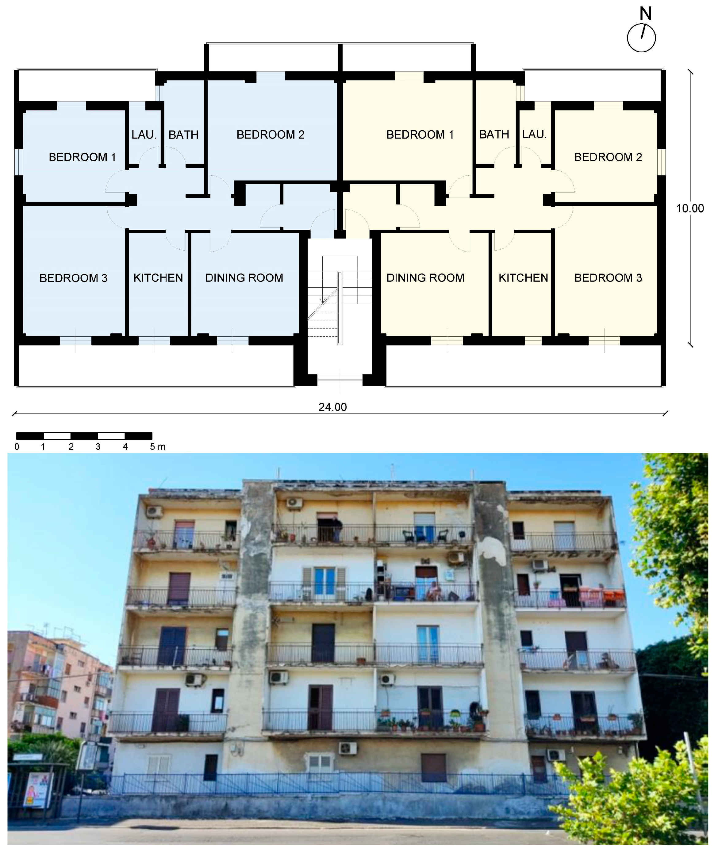
The present paper only deals with energy issues and only considers those data and KPIs regarding the building envelope; the simulation of the thermal systems will be addressed by a future separate paper. With the aim of demonstrating the capabilities of the tool, the e-DSS is here used to assess one existing building belonging to the local public housing institute in Catania, southern Italy. The main resulting KPIs are then compared against those obtained through detailed simulations with a certified commercial software tool used in Italy by professionals, both for the current building status and for its possible renovated configuration. This allows for identifying possible improvements to some algorithms within the e-DSS while also estimating the change in both the space heating and space cooling energy demand introduced by the e-SAFE renovation.

2. Materials and Methods

In the first part, this section presents the approach implemented in the e-DSS to manage the data input regarding the building geometry, the envelope components, and the weather data used for energy calculations. Then, Section 2.4 describes the equations used to calculate the energy needs for space heating and cooling. Finally, Section 2.5 shows how the e-DSS supports the evaluation of a renovation project and assists the user in assessing its energy performance.

2.1. Building Geometry

Coherently with the scope of having a tool that can be easily used during a preliminary design and evaluation stage, the introduction of the geometrical data is managed in a simplified way whilst still being able to reliably calculate the heat transfer area, the heated volume, and the heated floor area.

The main simplification consists of describing the building as a polygon with no more than eight sides, each identified through a subscript “i” associated with a different orientation (north = 1, northeast = 2, east = 3, southeast = 4, south = 5, southwest = 6, west = 7, northwest = 8). The user must introduce the length of the facade for each possible orientation (Length_i), the building height above the ground (H_tot), the total number of floors above the ground (n_floors), and the number of heated floors (n_heat). With these data, the e-DSS can already calculate the overall heated area of each facade (S_{heat_i}):

$$S_{heat\_i}={\displaystyle \frac{n_{heat}}{n_{floors}}}·\left({Length}_i·H_{tot}\right)$$

(1)

However, if there are other buildings adjacent to a certain facade, even if partially, the e-DSS assesses the heated area in contact with those adjacent buildings (S_{adj_i}):

$$S_{adj\_i}={\displaystyle \frac{n_{adj\_floors\_i}}{n_{heat}}}·S_{heat\_i}$$

(2)

Here, n_{adj_floors_i} is the number of heated floors that are in contact with an adjacent building on that facade, which is provided by the user for each orientation (n_{adj_floors_i} = 0 if there are no adjacent buildings on that orientation).

Then, it is necessary to separate the opaque surface area from the glazed surface area: to this aim, the user must specify the total window surface area (S_{w_i}) for each orientation, while the overall window surface area in the entire building is calculated as follows:

$$S_w={\sum }_{i=1}^8{S}_{w\_i}$$

(3)

Now, the “effective” heated vertical surface area in contact with the outdoors for each orientation (S_{eff_i}) is calculated through Equation (4), while the only opaque portion is defined with Equation (5):

$$S_{eff\_i}=S_{heat\_i}-S_{Adj\_i}$$

(4)

$$S_{eff\_op\_i}=S_{eff\_i}-S_{w\_i}-S_{box\_i}$$

(5)

In Equation (5), the surface area of the shutter boxes, if any, is roughly evaluated as 15% of the window’s surface, as in Equation (6); here, BOX is a Boolean variable introduced by the user (BOX = 1 if the building is provided with roller shutters; otherwise, BOX = 0).

$$S_{box\_i}=BOX·0.15·S_{w\_i}$$

(6)

Finally, the e-DSS needs to know the ground floor surface area (S_floor) and the roof surface area (S_roof). The first one is directly provided by the user as an input (it corresponds to the area of the base polygon); as far as the roof is concerned, it is calculated by the e-DSS by multiplying the ground floor area by a correction factor (f_roof):

$$S_{roof}=f_{roof}·S_{floor}$$

(7)

The correction factor depends on the type of roof selected by the user, making a choice between a flat surface (external roof or non-heated attic) and pitched surface (with a heated volume below), through a drop-down menu (see

Table 1. Drop-down menu for the boundary conditions of floors and roofs [15].

	Boundary Condition	${\mathit{b}}_{\mathit{t}\mathit{r}\_\mathit{U}}$	${\mathit{f}}_{\mathit{r}\mathit{o}\mathit{o}\mathit{f}}$
Floor of the first heated level	Basement with no windows	0.5	-
	Basement with windows	0.8	-
	Ground	0.45	-
	Outdoors	1	-
Roof of the last heated level	Outdoors (flat roof)	1	1
	Outdoors (pitched roof—low angle)	1	1.05
	Outdoors (pitched roof—high angle)	1	1.15
	Ventilated non-heated attic	1	1
	Uninsulated non-heated attic	0.9	1
	Insulated non-heated attic	0.7	1

). In the case of pitched surface, two slopes can be selected (low angle = around 20°, high angle > 30°).

The choice of a suitable boundary condition for both the roof and the ground floor introduces a further correction factor (b_{tr_U}) needed in the calculation of the heat transfer rate, as specified in Section 2.4. The various values are reported in Table 1 [15]. Finally, for all vertical surfaces attached to adjacent buildings, it is b_{tr_U_adj} = 0.

As a final piece of information about the geometry of the building, the user has to manually add the heated net floor area (S_net), the heated net volume (V_net) and the heated gross volume (V_g). In this stage, some checks are performed by the tool to avoid inappropriate input, eventually showing a warning:

• The heated gross volume cannot exceed the product of the ground surface area times the building height.
• Th ratio of the building height to the number of floors must be between 2.5 m and 5 m.
• The heated net volume must be within 60% to 90% of the heated gross volume.

Finally, the e-DSS calculates the compactness ratio (S/V), as per Equation (8):

$$S/V=S_{d\_tot}/V_g$$

(8)

Here, V_g is the gross heated volume of the building and S_{d_tot} is the overall heated envelope surface, given by Equation (9):

$$S_{d\_tot}=S_{floor}+S_{roof}+{\sum }_{i=1}^8{S}_{heat\_i}$$

(9)

2.2. Features of the Building Envelope Components

To describe the thermal performance of the building envelope components, it is necessary to insert their thermal transmittance (U-value). To this aim, the e-DSS already contains a predefined list of common opaque components with their corresponding U-value; the list is available through a drop-down menu, but the user can also decide to manually insert a different U-value if, for instance, this is already known from previous analyses. The list of the opaque structures implemented in the e-DSS is reported in Appendix A (

Table A1. Predefined U-values for the opaque envelope components (all values are in W∙m⁻²∙K⁻¹). The values are derived from preliminary research regarding building traditions in the three countries.

	Description	Italy	Greece	Romania
Wall	Solid brick wall	1.55	-	1.80
(Uwall)	Perforated bricks, tuff	1.35	2.20	1.32
	Uninsulated hollow bricks with air cavity	1.10	1.60	-
	Hollow bricks with partially insulated air cavity	0.80	0.85	0.92
	Prefabricated concrete walls	2.80	3.40	-
Floor	Uninsulated concrete slab	1.65 *	2.75	2.85
(Ufloor)	Uninsulated hollow-core concrete floor	1.25	1.20	1.15
	Insulated concrete slab	1.00	0.95	-
	Insulated hollow-core concrete floor	0.80	0.90	0.80
Roof	Flat uninsulated hollow-core concrete roof	1.50	-	1.15
(Uroof)	Pitched uninsulated hollow-core concrete roof	1.80	-	-
	Pitched uninsulated roof with wooden structure	1.80	3.20	-
	Uninsulated concrete slab	-	3.05	3.10
	Generic partially insulated roof	0.80	0.95	0.80

* In Italy, there is a significantly lower U-value because of the use of lightened concrete.

). The corresponding U-values are different for Italy, Greece, and Romania; these values have been defined through preliminary research conducted by local e-SAFE partners, who analyzed the most common assemblies and building materials used in the three countries until the end of the XX century.

The e-DSS follows a similar approach to define the U-values of the windows (U_w) by combining the features of both the glazed surface and the opaque frame (see

Table A2. Predefined U-values and solar transmission factors for the windows, as a function of the glazing type and the frame material (the same values are used in Italy, Greece, and Romania). The values are extracted from UNI/TS 11300-1:2014 [15].

Glazing	Frame	U-Value
Single glazing	Wood	4.9 W/(m2∙K)
(g-value = 0.85)	Metal	6.0 W/(m2∙K)
	Metal with thermal break	5.1 W/(m2∙K)
	PVC	5.0 W/(m2∙K)
	Wood and metal	5.2 W/(m2∙K)
Double glazing	Wood	2.8 W/(m2∙K)
(g-value = 0.75)	Metal	3.7 W/(m2∙K)
	Metal with thermal break	3.0 W/(m2∙K)
	PVC	2.9 W/(m2∙K)
	Wood and metal	3.1 W/(m2∙K)
Low-e double glazing	Wood	1.5 W/(m2∙K)
(g-value = 0.67)	Metal with thermal break	1.7 W/(m2∙K)
	PVC	1.3 W/(m2∙K)
	Wood and metal	1.7 W/(m2∙K)
Low-e triple glazing	Wood	1.0 W/(m2∙K)
(g-value = 0.50)	Metal with thermal break	1.1 W/(m2∙K)
	PVC	1.0 W/(m2∙K)
	Wood and metal	1.1 W/(m2∙K)

in Appendix A). By default, the frame occupies 30% of the window surface (frame factor $F_F$ = 0.3), which approximates the real features of many commercial windows. The thermal transmittance of the shutter boxes, if any, is set by default as U_box = 4 W/(m²∙K).

The presence of roller shutters also implies calculating the thermal transmittance of the windows when the shutters are closed (U_ws). The latter is determined according to UNI/TS 11300-1:2014 [15] by referring to a shutter with average air permeability:

$$U_{ws}={\left[{U_w}^{-1}+\left(0.55·R_{sh}+0.11\right)\right]}^{-1}$$

(10)

In Equation (10), R_sh is the additional thermal resistance of the closed shutter, whose possible values are R_sh = 0 m²∙K/W (metal shutter), R_sh = 0.15 m²∙K/W (wood or insulated plastic shutter) or R_sh = 0.1 m²∙K/W (other types of shutters). Finally, UNI/TS 11300-1:2014 determines the corrected window U-value (U_{w_corr}) considering that the shutters are closed during 60% of the day, as per Equation (11). Of course, if no roller shutter is selected, U_{w_corr} = U_w.

$$U_{w\_corr}=0.6·U_{w\mathrm{s}}+0.4·U_w$$

(11)

Moreover, to account for movable shading devices (e.g., blinds and curtains), the user can select an item from a drop-down menu, which implies a suitable shading factor:

• Inner light curtain: f_shade = 0.80;
• Outer light curtain: f_shade = 0.70;
• Other type of shading (inner side): f_shade = 0.55;
• Other type of shading (outer side): f_shade = 0.35.

The e-DSS also considers the color of the external finish for the vertical walls and the roof. The color determines the solar absorption coefficients, which are, respectively, identified as ${\alpha }_v$ and ${\alpha }_{hor}$; three possibilities are available (light = 0.3, medium = 0.6, and dark = 0.9), as suggested by UNI/TS 11300-1:2014 [15].

Finally, the user can specify whether a facade has balconies. Consequently, a projection factor (Fs_{h_i_j}) is attributed to the windows and the walls located in that facade. The value of the projection factor changes each month (“j”) coherently with the average sun height; the default values are taken from UNI/TS 11300-1:2014 and refer to an obstruction angle of 30° (typical of balconies) and latitude 42°00′ N (average recurring latitude in Italy, Greece, and Romania). If a facade has no balconies, Fs_{h_i_j} = 1 applies in all months.

2.3. Weather Data

The weather data necessary for the energy assessment of the building, according to the quasi-steady-state method adopted in the e-DSS and described in detail in the next section, are the monthly average of the dry-bulb air temperature (°C) and daily global solar irradiation (MJ/m²). Accordingly, the e-DSS tool automatically connects to the freeware online service PVGIS [16] and downloads the latest available year of data in the PVGIS-SARAH3 database for the location specified by the user through the latitude and the longitude. This database collects re-analysis data from satellite observations for Europe, Asia, Africa, and South America with a spatial resolution of about 5 km.

The data are downloaded in hourly format for one year and then directly averaged by the number of hours in the months in the case of air temperature, while for solar irradiation values, the hourly values (Wh/m²) are first summed up, then averaged by the number of days in the month, and eventually converted into MJ/m². This operation is performed for a horizontal surface (slope angle of 0°) and for eight vertical surfaces (slope angle of 90°), with azimuth angles changing by 45° step starting from south (0°).

2.4. Energy Calculations

The proposed approach to calculate the thermal energy needs for space heating and cooling is inspired by the quasi-steady-state method introduced by Italian national standard UNI/TS 11300-1:2014 and is today adopted by all commercial tools for building energy certification [15]. However, the attribution of some parameters has been simplified to make input data user-friendly, coherently with the scopes of the tool.

Equations (12) and (13) show the monthly thermal energy balances used to calculate the final thermal energy demand for space heating (Q_H) and space cooling (Q_C) under the hypothesis of continuous operation in standard conditions:

$$Q_{H\_j}=\left[Q_{H\_loss\_j}-{\mathsf{\eta }}_{\mathrm{H}\_\mathrm{g}\mathrm{n}\_\mathrm{j}}·Q_{H\_gain\_j}\right]·H_{days\_j}$$

(12)

$$Q_{C\_j}=\left[Q_{C\_gain\_j}-{\mathsf{\eta }}_{\mathrm{C}\_\mathrm{l}\mathrm{s}\_\mathrm{j}}·Q_{C\_l\mathrm{o}\mathrm{s}\mathrm{s}\_\mathrm{j}}\right]·C_{days\_j}$$

(13)

Here, the subscript “j” refers to each month (j = 1 ÷ 12). The duration in days of the months included in the heating season ($H_{days\_j}$) and in the cooling season ($C_{days\_j}$), as well as the relations to calculate the utilization factors ${\eta }_{H\_gn\_j}$ and ${\eta }_{C\_ls\_j}$, will be introduced in Section 2.4.4. From now on, this section will detail only the equations relating to the space heating needs. However, they are also applicable in the cooling season, apart from some slight differences that will be duly underlined.

In Equation (12) and Equation (13), the daily heat losses and heat gains are calculated as per Equation (14) and Equation (15), respectively. The single terms are commented on hereafter.

$$Q_{H\_loss\_j}=Q_{H\_tr\_j}+Q_{H\_ve\_j}-Q_{H\_sol\_op\_j}$$

(14)

$$Q_{H\_gain\_j}=Q_{H\_end\_j}+Q_{H\_sol\_w\_j}$$

(15)

2.4.1. Transmission Heat Losses

For each month “j” included in the heating period, the daily thermal energy transmitted through the building envelope is:

$$Q_{H\_tr\_j}=24·\left[H_{tr}·\left({\theta }_{HEAT}-{\theta }_{e\_j}\right)+{11·\mathrm{\varnothing }}_{r\_tot}\right]/1000$$

(16)

Here, ${\theta }_{e\_j}$ is the monthly mean outdoor air temperature, determined as explained in Section 2.3, while ${\theta }_{HEAT}$ is the indoor temperature setpoint, set by the user through a specific drop-down menu (this is expressed as ${\theta }_{COOL}$ in the cooling season). The total radiant heat exchange with the sky is determined as per Equation (17):

$${\mathrm{\varnothing }}_{r\_tot}=ROOF·{\mathrm{\varnothing }}_{r_{\mathrm{r}\mathrm{o}\mathrm{o}\mathrm{f}}}+0.5·{\sum }_{i=1}^8{\mathrm{\varnothing }}_{r\_\mathrm{i}}$$

(17)

Here, ROOF is a Boolean variable (ROOF = 1 if the type of boundary condition selected for the roof corresponds to “Outdoors”; otherwise, ROOF = 0). Moreover, given the thermal resistance associated with the outside surface heat transfer ($R_{se\_ho}=R_{se\_\mathrm{v}}=0.04$ m²∙K/W) [17], one can calculate the following [18]:

$${\mathrm{\varnothing }}_{r\_\mathrm{r}\mathrm{o}\mathrm{o}\mathrm{f}}=R_{se\_ho}·4.14·S_{roof}·U_{roof}$$

(18)

$${\mathrm{\varnothing }}_{r\_\mathrm{i}}=R_{se\_v}·4.14·(S_{eff\_op\_i}·U_{wall}+S_{box\_i}·U_{box}+S_{w\_i}·U_{w\_corr})$$

(19)

Back to Equation (16), the transmission heat loss coefficient (H_tr, in W/K) is:

$$H_{tr}=H_{tr\_floor}+H_{tr\_roof}+{\sum }_{i=1}^8{H}_{tr\_i}$$

(20)

As far as the vertical surfaces are concerned, the e-DSS the following calculates for each orientation:

$$H_{tr\_i}=c_{th}·\left[S_{eff\_op\_i}·U_{wall}+S_{w\_i}·U_{w\_corr}+S_{box\_i}·U_{box}+S_{adj\_i}·U_{wall}·b_{tr\_U\_adj}\right]$$

(21)

Here, the correction coefficient (c_th) considers—in a simplified way—the role of the thermal bridges. Several cases may occur, according to the presence of balconies:

• If there are no balconies: c_th = 1.1;
• If the balconies are just on one facade: c_th = 1.2;
• If the balconies are on two facades: c_th = 1.3;
• If the balconies are on three facades: c_th = 1.35;
• If the balconies are on four or more facades: c_th = 1.4.

Similarly, the e-DSS calculates the transmission heat loss coefficient in relation to the floor and the roof according to Equation (22) and Equation (23), respectively:

$$H_{tr\_floor}=c_{th}·S_{floor}·U_{floor}·b_{tr\_U\_floor}$$

(22)

$$H_{tr\_roof}=c_{th}·S_{roof}·U_{roof}·b_{tr\_U\_roof}$$

(23)

In these equations, the correction coefficient is by default c_th = 1.1 because the thermal bridges occurring in horizontal envelope surfaces are usually not as impactive as in vertical walls with balconies. Finally, the e-DSS determines the transmission heat loss coefficient per unit heated envelope surface, recalled in several national regulations:

$${H^{\prime }}_T=H_{tr}/S_{d\_tot}$$

(24)

2.4.2. Ventilation Heat Losses

The daily heat transfer by ventilation is calculated as per Equation (25), where the ventilation heat loss coefficient (H_ve, in W/K) is derived from Equation (26) [15]:

$$Q_{H\_ve\_j}=24·\left[H_{ve}·\left({\theta }_{HEAT}-{\theta }_{e\_j}\right)\right]/1000$$

(25)

$$H_{ve}=0.34·\left[V_{net}·ACH·RES+\left(1-RES\right)·3.6·L_{ps}·f_{ve}·P_{sqm}·S_{net}·C2\right]·(1-REC)$$

(26)

In Equation (26), V_net is the net volume of the heated zones, and S_net is the overall net floor surface of the building. Both values are assigned during the definition of the building geometry. Furthermore, the air exchange rate is assigned as a function of the intended building use: in residential buildings, ACH = 0.3 h⁻¹, while in other type of buildings, one has to know the nominal ventilation rate per person in L/s (L_ps), the occupancy rate in people/m² (P_sqm), and the correction factor (f_ve) that accounts for the possibility that mechanical ventilation is not exploited all day long. Their values are reported in Appendix A (

Table A3. Standard values for endogenous heat (θ_END), occupancy rate (P_sqm), and ventilation parameters, according to the predominant building use.

Predominant Building Use	θEND	Psqm	Lps	fve
	(W∙m−2)	(people∙m−2)	(L∙s−1∙person−1)	(-)
Residential	4.5	0.05	-	-
Library	8.0	0.30	6.0	0.51
Hotel	6.0	0.05	11.0	0.26
Offices	6.0	0.06	11.0	0.59
Hospital	8.0	0.08	11.0	1.00
Cinema/theater	8.0	1.00	5.5	0.51
Museum/church	8.0	0.30	6.0	1.00
Restaurant	10.0	0.60	10.0	0.47
Commercial building	8.0	0.20	9.0	0.51
Swimming pool	10.0	0.30	2.5	0.34
Gym	5.0	0.20	6.0	0.18
School	4.0	0.45	5.0	0.47
Industrial building	6.0	-	-	-

) [15]. The coefficient C2 depends on the altitude of the location (see

Table 2. Values for the correction coefficient C2 [15].

Altitude (H)	C2
H < 500 m	1.00
500 m < H < 1000 m	1.06
1000 m < H < 1500 m	1.12
1500 m < H < 2000 m	1.18
2000 m < H < 2500 m	1.25

). RES is a Boolean variable: RES = 1 if the predominant building use is “Residential”, while RES = 0 in all other cases. Finally, REC is the efficiency of the heat recovery unit in the case of a controlled mechanical ventilation system (REC = 0 if no heat recovery unit is provided, and REC = 0.8 by default if the user does not know the exact value).

2.4.3. Solar Gains Through Windows and Opaque Components

The mean daily value of the solar gains through windows ($Q_{H\_sol\_w\_j}$, in kWh/day) is determined as:

$$Q_{H\_sol\_w\_j}={f_{shade}·g}_{factor}·{\sum }_{i=1}^8\left(I_{sol\_i\_j}·S_{w\_i}·F_{sh\_i\_j}\right)·\left(1-F_F\right)/3.6$$

(27)

In Equation (27), $g_{factor}$ is the solar transmission factor of the glazed surface, automatically attributed according to the glazing type (Table A2), and $I_{sol\_i\_j}$ is the monthly mean of the daily global solar irradiation (MJ/m²) for the “i-th” orientation and the “j-th” month.

The mean daily value of the solar gains absorbed by the opaque envelope components ($Q_{H\_sol\_\mathrm{o}\mathrm{p}\_j}$, in kWh/day) is determined as:

$$Q_{H\_sol\_op\_j}=\left[\begin{array}{c}\sum _{i=1}^8\left(I_{sol\_i\_j}·(S_{eff\_op\_\mathrm{i}}·U_{wall}+S_{box\_\mathrm{i}}·U_{box}\right)·R_{se\_v}·{\alpha }_v)+\\ +ROOF·I_{sol\_\mathrm{h}\mathrm{o}\mathrm{r}\_j}·S_{roof}·U_{roof}·R_{se\_ho}·{\alpha }_{ho}\end{array}\right]/3.6$$

(28)

Here, $I_{sol\_hor\_j}$ is the monthly average of the daily global solar irradiation on the horizontal plane (MJ/m²) for the j-th month.

2.4.4. Endogenous Heat and Utilization Factors

The endogenous heat is determined as:

$$Q_{H\_end\_j}=(24·{\theta }_{END}·S_{net})/1000$$

(29)

Here, ${\theta }_{END}$ is the average thermal power released by endogenous heat sources (people, electric appliance, artificial lighting) per unit net surface, whose values depend on the intended building use (

Table A4. Values of the projection factor (F_{sh_i_j}) associated with the balconies, according to the orientation of the facade.

Month		North (i = 1)	Northeast (i = 2)	Southeast (i = 4)
			East (i = 3), West (i = 7)	South (i = 5)
			Northwest (i = 8)	Southwest (i = 6)
January	(j = 1)	0.80	0.87	0.88
February	(j = 2)	0.80	0.84	0.84
March	(j = 3)	0.80	0.82	0.78
April	(j = 4)	0.80	0.80	0.70
May	(j = 5)	0.83	0.79	0.65
June	(j = 6)	0.82	0.77	0.63
July	(j = 7)	0.83	0.78	0.61
August	(j = 8)	0.81	0.78	0.66
September	(j = 9)	0.80	0.82	0.74
October	(j = 10)	0.80	0.84	0.82
November	(j = 11)	0.80	0.86	0.87
December	(j = 12)	0.80	0.87	0.89

).

Moreover, the first step to calculate the utilization factors ${\eta }_{H\_gn\_j}$ and ${\eta }_{C\_ls\_j}$ consists of evaluating the time constant (tau) of the building, measured in hours:

$$tau=(S_{d_{tot}}·C_{mean}/3600)/\left[\right(H_{tr}+H_{ve})/1000]$$

(30)

In Equation (30), C_mean is the mean thermal capacity per unit surface of opaque heated envelope. This parameter is attributed based on the type of wall selected by the user (see Table A1), and its value is either 135 kJ/(m²∙K) in the case of heavy structures (concrete walls, tuff, solid bricks) or 120 kJ/(m²∙K) otherwise [15].

Once the time constant is known, the gains utilization factor in the heating season is determined for each j-th month as:

$${\eta }_{H\_GN\_j}=min \left({\displaystyle \frac{1-{{\gamma }_{H\_j}}^{a_H}}{1-{{\gamma }_{H\_j}}^{(a_H+1)}}};1\right)$$

(31)

where:

$$a_H=1+{\displaystyle \frac{tau}{15}} {\gamma }_{H\_j}=max\left(Q_{H\_gain\_j}/Q_{H\_loss\_j};0\right)$$

(32)

Finally, the duration of the heating season corresponds to all those months in which the condition in Equation (33) holds. If the condition is true, H_days in Equation (12) is the number of the days in that month; otherwise, H_days = 0.

$$\left[{\gamma }_{H\_j}<{(a}_H+1)/a_H\right] AND \left[{\gamma }_{H\_j}\ne 0\right]$$

(33)

Similarly, in the cooling season, the utilization factor for the heat losses is:

$${\eta }_{C\_ls\_j}=min\left({\displaystyle \frac{1-{{\gamma }_{C\_j}}^{-a_C}}{1-{{\gamma }_{C\_j}}^{({-a}_C-1)}}};1\right) with {\gamma }_{C\_j}>0$$

(34)

where:

$$a_C=\mathit{max}\left[\left(8.1+{\displaystyle \frac{tau}{17}}-13· {\displaystyle \frac{S_w}{S_{net }}}\right);0\right] {\gamma }_{C\_j}=Q_{C\_gain\_j}/Q_{C\_loss\_j}$$

(35)

The duration of the cooling season corresponds to those months in which the condition in Equation (36) holds. If the condition is true, C_days in Equation (13) is the number of the days in that month; otherwise, C_days = 0.

$${\left({\gamma }_{C\_j}\right)}^{-1}<{(a}_C+1)/a_C$$

(36)

2.5. Renovation Stage

The e-DSS does not aim at calculating or certifying the seismic improvement provided by the possible renovation solutions, since this outcome would need the use of specific tools for a dynamic structural analysis. However, the e-DSS assists the technician in the preliminary decision-making process towards the most suitable e-SAFE solution for energy-and-seismic improvement, considering the height and shape of the building, the current state of conservation of the RC structures, and the seismic zone.

Thus, the user can initially select if he/she wants to go for an energy-and-seismic renovation. In this case, the e-DSS poses a series of questions, such as:

• Level of degradation of the existing structures (no degradation, just slightly degraded, degraded but they can be easily recovered, too degraded);
• Percentage of perimeter occupied by balconies in a typical floor;
• Number of facades attached to other buildings;
• Number of floors;
• Presence of constraints that prevent altering the appearance of the building (e.g., local regulations, cultural heritage restrictions);
• Availability of sufficient space for crane operations around the building.

The seismicity of the city where the building is located depends on the Peak Ground Acceleration (PGA), automatically retrieved through the EFEHR web service [19].

Based on the above data, the e-DSS attributes a score to the building and determines the most suitable combined energy-and-seismic renovation solution (e-CLT or e-EXOS). In some cases, the e-DSS might exclude one or even both solutions, which happens, for instance, if the number of floors is above twelve or when local regulations forbid altering the facade. Further details are available in the relevant e-SAFE project’s deliverable [20].

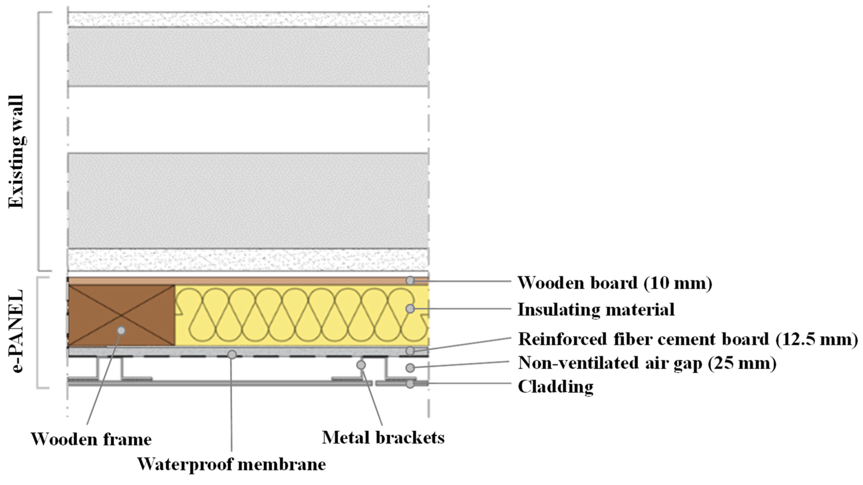
After this preliminary decision stage, if the user chooses either a simple energy renovation (no seismic improvement) or a combined energy-and-seismic renovation relying on e-EXOS, the tool considers e-PANEL as the only candidate solution to improve the envelope’s energy performance. A typical cross-section of an e-PANEL applied to an existing wall is depicted in Figure 1. Here, the non-insulated wooden frame covers approximately 30% of the total e-PANEL surface, based on a series of detailed design experiences conducted so far.

Accordingly, the e-DSS calculates the mean U-value of the wall renovated through the e-PANEL (U_{wall_new}) as follows:

$$U_{wall\_new}=0.7\cdot U_{PANEL}+0.3\cdot U_{frame}$$

(37)

where:

$$U_{PANEL}={\left({\displaystyle \frac{1}{U_{wall}}}+{\displaystyle \frac{0.01}{{\lambda }_{wood}}}+{\displaystyle \frac{{\delta }_{ins}}{{\lambda }_{ins}}}+{\displaystyle \frac{0.0125}{{\lambda }_{fib}}}+R_{GAP}+{\displaystyle \frac{{\delta }_{clad}}{{\lambda }_{clad}}}\right)}^{-1}$$

(38)

$$U_{frame}{=\left({\displaystyle \frac{1}{U_{wall}}}+{\displaystyle \frac{{\delta }_{ins }+0.01}{{\lambda }_{wood}}}+{\displaystyle \frac{0.0125}{{\lambda }_{fib}}}+R_{GAP}+{\displaystyle \frac{{\delta }_{clad}}{{\lambda }_{clad}}}\right)}^{-1}$$

(39)

The above equations rely on the following positions:

• The wooden frame has the same thickness as the insulation layer.
• The wooden frame and the wooden board behind the insulation have default thermal conductivity λ_wood = 0.13 W/(m∙K).
• The thermal resistance of the scarcely ventilated air gap behind the cladding is R_GAP = 0.09 m²∙K/W [17].
• The fiber cement board has default thermal conductivity λ_fib = 0.32 W/(m∙K).
• The thermal resistance of the metal brackets and the water-proof membrane, necessary to reduce the risk of moisture accumulation, is negligible [21].
• The type of cladding can be selected from a drop-down menu (Appendix A,

  Table A5. Default features for insulating and cladding materials used in the renovation stage.

  Insulating Material	λ (W∙m−1∙K−1)	Cladding Material	λ (W∙m−1∙K−1)	δ (mm)
  Wooden fiber	0.04	Fiber cement (with plaster)	0.32	15
  Cellular glass	0.055	Fiber cement (without plaster)	0.32	15
  Hemp fiber	0.038	Pre-painted aluminum	200	2
  Cellulose fiber	0.037	Wooden slats	0.13	20
  Sheep wool	0.035	WPC slats	0.13	20
  Rock wool	0.036	Clay slats	0.4	15
  EPS	0.037	Porcelain stoneware	1.0	15
  XPS	0.035	Ceramic/clay	1.0	15
  Cork	0.039

  ), which automatically sets δ_clad and λ_clad.

Now, when the user decides to simulate a renovation scenario relying on the e-PANEL, the main step consists of setting the insulation type and thickness. The type of material can be chosen from a drop-down menu including the options available in Appendix A (Table A5), each associated with a design conductivity value [22]. Moreover, the user must set the insulation thickness (δ_ins) wisely, because in the case of energy renovation, many European countries require that a threshold U-value is not overcome (

Table 3. Maximum U-values allowed for the vertical walls in case of building renovation (all values are in W∙m⁻²∙K⁻¹) [23].

Climatic Zone	Italy	Greece	Romania *
Zone A	0.40	0.60	-
Zone B	0.40	0.50	-
Zone C	0.36	0.45	-
Zone D	0.32	0.40	-
Zone E	0.28	-	-
Zone F	0.26	-	-

* In Romania, the recommended U-value for walls in the case of building renovation is U = 0.33 W∙m⁻²∙K⁻¹, independently on the climatic zone.

).

To this aim, the e-DSS automatically calculates the minimum thickness needed to comply with this legal requirement, knowing the country where the building is and the climatic zone, if relevant. Indeed, the e-DSS operates a “while” loop, where the insulation thickness is increased by 2 cm steps and Equations (37)–(39) are solved until the resulting U_{wall_new} becomes lower than the relevant threshold. Then, the e-DSS notifies the result, and the user can either confirm it or choose an even higher insulation thickness; in the second case, the e-DSS calculates the final U_{wall_new} again and assigns it to all walls in the building to calculate the new energy performance.

Then, the user might also want to include a roof renovation. In this case, the e-DSS allows for selecting the desired insulation (drop-down menu in Table A5) and its thickness (δ_{ins_roof}), so that it can calculate the new thermal transmittance (U_{roof_new}) assigned to the roof surface in place of U_roof:

$$U_{roof\_new}={\left({\displaystyle \frac{1}{U_{roof}}}+{\displaystyle \frac{{\delta }_{ins\_roof}}{lambd{a}_{ins\_r}}}+0.1\right)}^{-1}$$

(40)

Here, the additional thermal resistance R = 0.1 m²∙K/W accounts for both the new tiles and the lightweight cement screed layer between the insulation and the tiles, with an overall thickness of around 5 cm and an average thermal conductivity around 0.5 W/(m∙K). In this stage, the user can also select the type of tiles and the presence of a weather-protection membrane; however, this choice does not affect energy performance.

As far as thermal bridges are concerned, the correction coefficient (c_th) used in Equation (21) assumes different values compared to the pre-renovation stage, since thermal bridges are partially corrected by the outer thermal insulation:

• If there are no balconies: c_th = 1.1;
• If the balconies are just on one facade: c_th = 1.125;
• If the balconies are on two facades: c_th = 1.15;
• If the balconies are on three facades: c_th = 1.175;
• If the balconies are on four or more facades: c_th = 1.2.

Coming to the glazed components, the proposed renovation solution implies that they are replaced by new high-performing windows mounted in a suitably shaped e-PANEL. The glazing type is set by default as low-e double glazing, but the user can select the type of frame; consequently, the e-DSS sets the new U-value (U_{w_new}) according to Table A2. The user can also choose to manually insert the new U-value if it is known from technical datasheets; in any case, g_{factor_new} = 0.67 is used by default.

The new windows also include outer shading devices, whose shading factor is set by default to f_shade = 0.35. Furthermore, the new windows are not provided with shutter boxes; so, if the existing windows had shutter boxes, in the renovation stage, the e-DSS would set S_BOX = 0 in Equations (21) and (28), and the window surface would be increased by 15%.

3. Case Study

3.1. Building Geometry and Features

The building taken as a case study is situated in Catania (southern Italy), its construction dates to the 1960s, and it is part of the local public residential stock. It consists of five floors with two flats per floor, with an RC structural frame and cavity walls with two layers of lightweight concrete blocks. The roof is flat and uninsulated, while a floor slab separates the ground floor from an inaccessible, hollow basement that prevents rising damp. Balconies are present on the two main fronts, facing south and north; most of the glazed surface lies on these fronts, while only few small windows are in the east and west fronts. Almost all windows have double glazing and metal frames with no thermal break, roller shutters, and uninsulated boxes, while only a few windows have single clear glasses. Finally, there are no adjacent buildings (n_{adj_floors} = 0). Figure 2 shows the typical plan of the building, including an internal condominium staircase, and a picture of the main facade.

Table 4. Building features used as input in the e-DSS.

Parameter	Value
Year of construction	1964
Coordinates	Lat = 37.49°, long = 15.08°
Altitude	H = 7 m
Climatic zone	B
Number of dwellings	10
Winter indoor set-point temperature	θHEAT = 20 °C
Summer indoor set-point temperature	θCOOL = 26 °C
Number of floors	nfloors = 5
Number of heated floors	nheat = 5
Building height	Htot = 16.9 m
Gross surface of the ground floor	Sfloor = 231 m2
Heated net floor area	Snet = 940 m2
Window surface (N-E-S-W)	Sw = 58.9 m2–11.7 m2–83.5 m2–11.7 m2
Overall net heated volume	Vnet = 2630 m3
Overall gross heated volume	Vg = 3454 m3
Color of the external finish	Medium
U-value of the walls	Uwall = 1.00 W∙m−2∙K−1
U-value of the windows	Uw = 3.00 W∙m−2∙K−1
Existing roller shutters	Wood or plastic
Shading devices	Inner light curtains (fshade = 0.80)
Presence of balconies	North and south facades
U-value of the roof	Uroof = 1.30 W∙m−2∙K−1
Roof boundary condition	Outdoors (flat roof)
U-value of the floor slab	Ufloor = 0.64 W∙m−2∙K−1
Boundary condition for the floor slab	Basement with no windows

contains all the input data used in the e-DSS, retrieved both from the available design documents (plans, fronts) and through on-site surveys. The length of the facades was taken by assuming a slightly simplified shape, i.e., by excluding the projection of the stairwell.

In the renovation stage, the e-PANEL will have δ_ins = 8 cm, leading to U_{wall_new} = 0.36 W∙m⁻²∙K⁻¹, below the maximum value set by law in Zone B (Table 3). The roof will be insulated by 10 cm of wood fiber, with a resulting U_{roof_new} = 0.30 W∙m⁻²∙K⁻¹. New windows have a timber frame and low-e double glazing, with U_{w_new} = 2.3 W∙m⁻²∙K⁻¹.

3.2. Simulation with a Commercial Tool

The case study was simulated not only with the e-DSS but also with Blumatica Energy [24], a commercial certified tool widely used by professionals in Italy for building energy certification, thus allowing for comparing the results from both tools and assessing the reliability of the e-DSS.

Table A6. Thermal features of external walls (from the inner to the outer side)—U = 1.00 W/(m²K).

Material	s (m)	λ (W∙m−1∙K−1)	Cp (J∙kg−1∙K−1)	ρ (kg∙m−3)	R (m2∙K∙W−1)
Surface thermal resistance	-	-	-	-	0.13
Gypsum plaster	0.02	0.57	1000	1300	0.035
Hollow concrete blocks	0.08	0.29	1000	845	0.276
Non-ventilated air gap	0.09	0.50	1000	1.2	0.180
Cement mortar	0.01	1.40	1000	2000	0.007
Hollow concrete blocks	0.12	0.39	1000	667	0.307
Lime and cement plaster	0.03	0.90	840	1800	0.033
Surface thermal resistance	-	-	-	-	0.04

and

Table A7. Thermal features of the roof (from the top to the bottom side)—U = 1.30 W/(m²K).

Material	s (m)	λ (W∙m−1∙K−1)	Cp (J∙kg−1∙K−1)	ρ (kg∙m−3)	R (m2∙K∙W−1)
Surface thermal resistance	-	-	-	-	0.170
Exterior floor tiles	0.02	0.57	1000	1300	0.035
Cement mortar	0.20	0.64	840	1132	0.310
Cement screed	0.14	0.58	1000	1400	0.241
Cement mortar	0.02	1.40	1000	2000	0.014
Concrete and clay blocks	0.02	0.70	1000	1500	0.029
Indoor plaster	-	-	-	-	0.040
Surface thermal resistance	-	-	-	-	0.170

in Appendix A describe the wall and roof assemblies used in the simulation with Blumatica Energy. It is worth mentioning that Blumatica Energy also performs a detailed analysis of all thermal bridges, based on their geometry and the materials included in the opaque components.

One key aspect is that the two tools use different weather data to calculate the building’s energy needs. Indeed, Blumatica Energy adopts the official weather data available in the Italian standard UNI 10349-1:2016 [25], while the e-DSS follows the approach already described in Section 2.3. The reason for this choice is that the e-DSS should in principle be used in every location worldwide, and using official weather databases for many different countries would mean a huge preliminary implementation work.

Table 5. Monthly mean dry-bulb air temperature in Catania: comparison between UNI 10349-1:2016 (used by Blumatica) and PVGIS (used by the e-DSS).

Month	UNI 10349-1	PVGIS (2023)	Difference
January (heating season)	11.9 °C	11.0 °C	−0.9 °C
February (heating season)	10.4 °C	10.5 °C	+0.1 °C
March (heating season)	11.8 °C	13.4 °C	+1.6 °C
April	15.4 °C	15.1 °C	−0.3 °C
May	18.8 °C	18.0 °C	−0.8 °C
June (cooling season)	23.4 °C	23.5 °C	+0.1 °C
July (cooling season)	25.8 °C	29.6 °C	+3.8 °C
August (cooling season)	26.5 °C	27.5 °C	+1.0 °C
September (cooling season)	22.9 °C	24.8 °C	+1.9 °C
October	19.8 °C	22.6 °C	+2.8 °C
November	15.1 °C	17.2 °C	+2.1 °C
December (heating season)	12.3 °C	12.9 °C	+0.6 °C

and Figure 3 compare the main data taken from the two different sources for the city of Catania, using 2023 as the reference year for PVGIS. The year 2023 was selected to represent the PVGIS climatic data, as it was identified as one of the most representative years based on an analysis of the last 15 years available in the software (from 2009 to 2023). The relevance of the selected year is demonstrated in Figure 4, where it can be observed that, for most months, 2023 closely aligned with the median values both in terms of temperature and solar irradiance. The biggest differences in the mean air temperatures occurred in July and September, and in both cases, PVGIS provides higher values than UNI 10349-1:2016 (by 3.8 °C and 1.9 °C, respectively). In the heating season, March is the month showing the highest discrepancy, with PVGIS providing a higher mean temperature by 1.6 °C. The discrepancy between the mean daily global irradiation is usually below 10%, except for the north facade (PVGIS systematically underestimates this by around 50%) and the south facade in the winter (PVGIS overestimates this by around 70%).

4. Results and Discussion

4.1. Comparison Between e-DSS and Blumatica Energy

To investigate the reliability of the e-DSS in estimating heat losses and heat gains during both the heating and cooling seasons, this section compares the outcomes from the two software tools. It is important to note that this comparison should not be considered a ‘validation’ process due to the different weather datasets employed by each tool, as outlined in Section 3.2.

As a first result,

Table 6. Comparison of some geometry-based parameters calculated in Blumatica and the e-DSS.

Parameter	Unit	Blumatica	e-DSS	Difference
Overall heated envelope surface (Sd_tot)	m2	1670.1	1638.6	−1.9%
Gross dispersing volume	m3	3501.0	3457.0	−1.3%
Compactness ratio (S/V)	m−1	0.477	0.474	−0.6%
Frame factor (FF)	-	0.72	0.7	−2.8%
Transmission heat loss coefficient (H′T)
Before renovation	W∙m−2∙K−1	1.44	1.39	−3.5%
After renovation	W∙m−2∙K−1	0.63	0.60	−4.7%

proves that the e-DSS calculated the main geometric outputs—overall heated envelope surface and compactness ratio—with good accuracy, despite its simplified approach. The transmission heat loss coefficient was slightly underestimated both before and after renovation; however, in both cases, the discrepancy was below 5%. This result is very satisfying if one considers the simplified approach to assess thermal bridges, based on correction coefficients that depend on the number of facades with balconies.

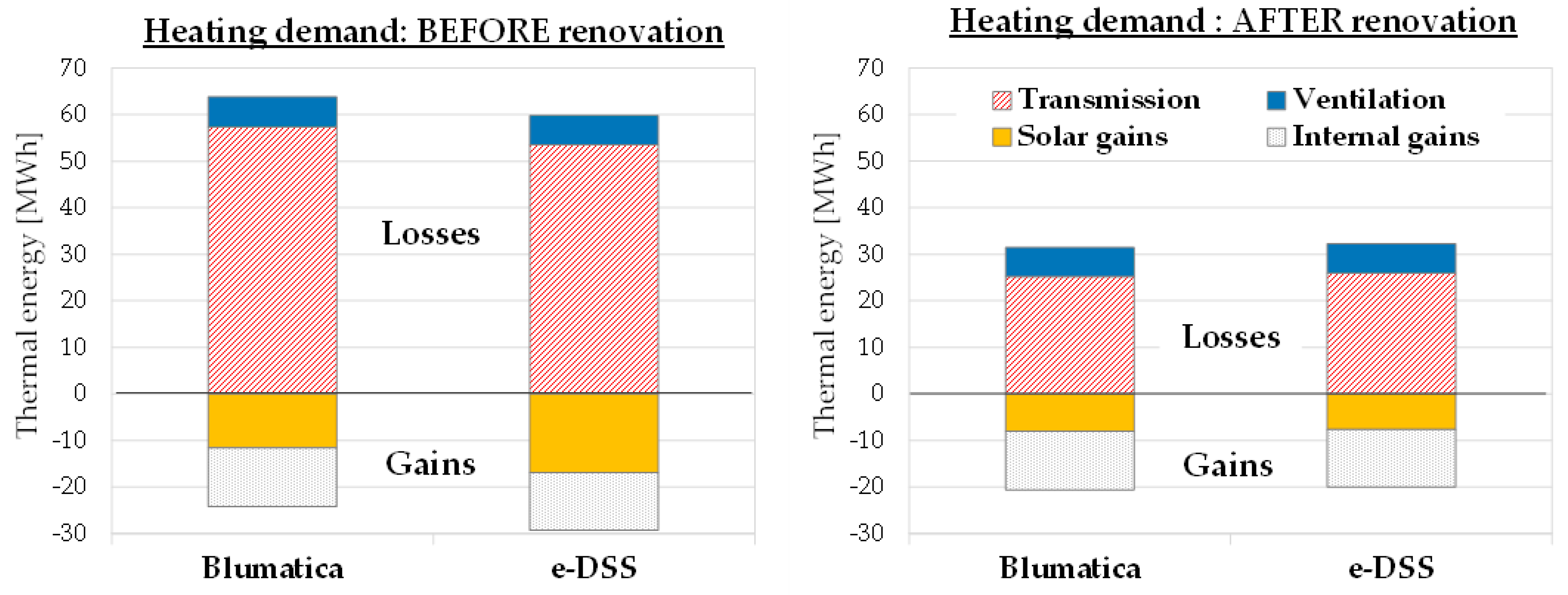
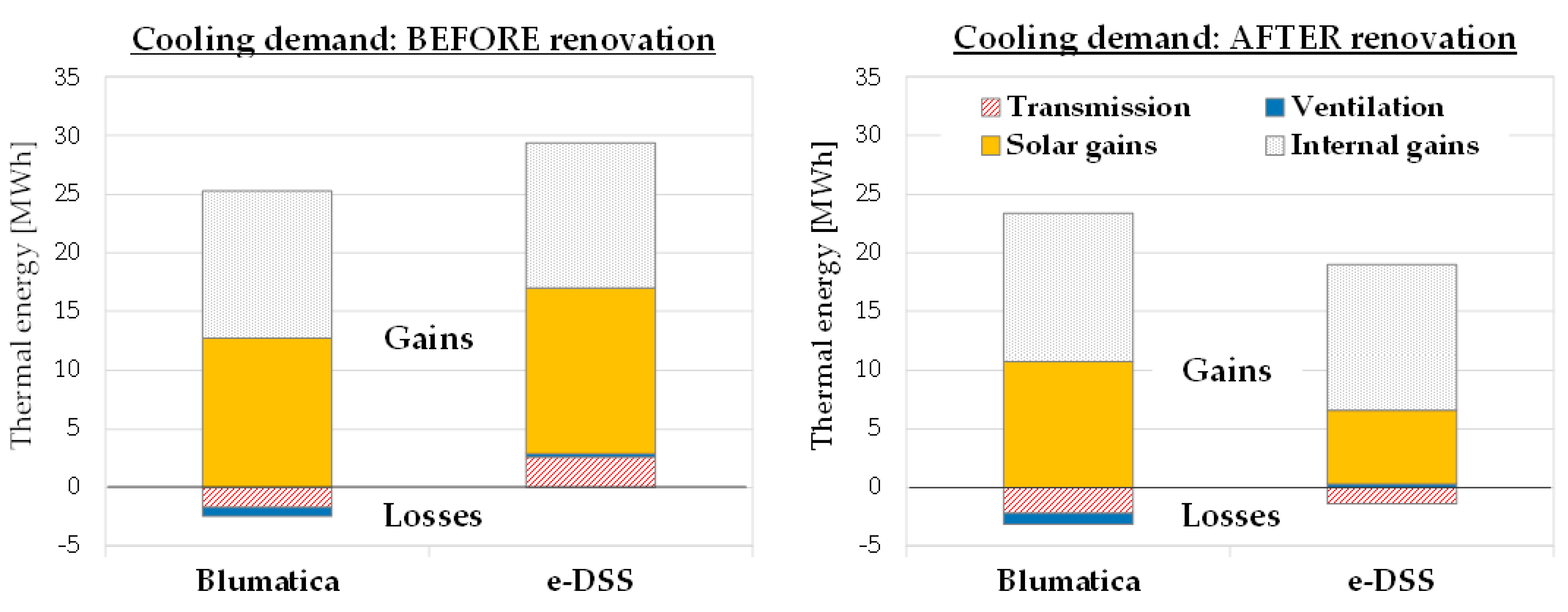
Then, Figure 5 and Figure 6 and

Table 7. Heat gains and heat losses: comparison between the two tools in both seasons.

	Heating Demand (Winter)
Parameter	BEFORE e-SAFE Renovation			AFTER e-SAFE Renovation
	Blumatica	e-DSS	Δ	Blumatica	e-DSS	Δ
QH	41.0 MWh	32.9 MWh	−19.8%	12.7 MWh	14.0 MWh	+10.5%
QH_loss	63.8 MWh	59.8 MWh	−6.3%	31.6 MWh	32.3 MWh	+2.2%
QH_gain	24.2 MWh	29.1 MWh	+20.2%	20.6 MWh	19.8 MWh	−3.9%
ηH_gn	0.942	0.925	−1.8%	0.917	0.922	+0.5%
	Cooling Demand (Summer)
Parameter	BEFORE e-SAFE Renovation			AFTER e-SAFE Renovation
	Blumatica	e-DSS	Δ	Blumatica	e-DSS	Δ
QC	23.2 MWh	29.4 MWh	+26.9%	20.6 MWh	17.5 MWh	−14.8%
QC_gain	25.6 MWh	26.5 MWh	+3.5%	23.7 MWh	18.7 MWh	−21.1%
QC_loss	2.4 MWh	−2.9 MWh	−218.4%	3.1 MWh	1.1 MWh	−65.1%
ηC_ls	0.991	0.996	+0.1%	0.995	0.996	-

provide the details of the terms that concur in the calculation of space heating and cooling demand, both before and after renovation.

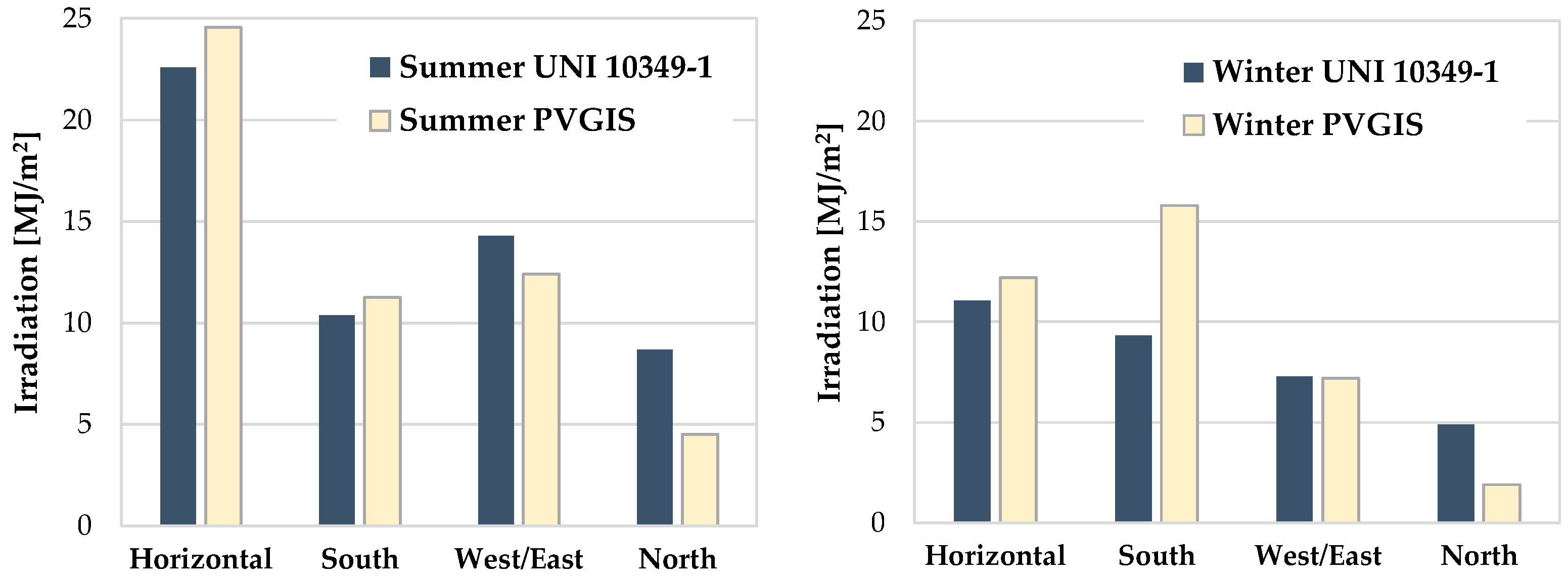
Starting from the heating demand (Figure 5), in the current building configuration (before renovation), the main discrepancy concerns the solar gains; indeed, the e-DSS overestimated them by 45%, which is coherent with the difference in the mean global irradiation values reported in winter by the two weather datasets for the south orientation (Figure 3), i.e., the orientation with the greatest glazed surface. Instead, internal gains were just slightly underestimated (−4%) compared with Blumatica Energy. Heat losses by ventilation showed very good accordance (−1.6%), whereas the e-DSS underestimated heat losses by transmission by 6.8%; this is coherent with the difference in the transmission heat loss coefficients observed in Table 6 but also stems from the mean monthly outdoor air temperatures in the winter months (Table 5) that were—on average—higher in the e-DSS than in Blumatica Energy, thus providing a lower temperature drop between indoors and outdoors. Overall, the space heating demand calculated by the e-DSS underestimated the result provided by Blumatica Energy by 19.8%.

Still looking at the heating demand (Figure 5), the previously outlined differences became less important in the building after renovation because the low U-values and the presence of effective movable shading devices reduced the effects of the different weather data. Thus, in this case, the e-DSS overestimated the heating demand by 10.5%, with the solar gains being underestimated by just 5%. The calculation of internal gains and heat losses by ventilation maintained very good reliability.

The calculation of the cooling demand (Figure 6) presents different outcomes that can be partially justified by the different weather data. Indeed, the monthly mean outdoor air temperature values retrieved from PVGIS are constantly higher than the corresponding data used by Blumatica Energy and—in July and August—also above the indoor set-point temperature (26 °C). For this reason, in the e-DSS, heat losses by ventilation and transmission turned into heat gains, thus contributing to increasing the cooling demand, while Blumatica considered these terms as heat losses that reduced the cooling demand. Furthermore, there is a difference in the mean global irradiation values reported in the summer by the two weather datasets for the south orientation, which is, however, not as high as in the winter (Figure 3), which makes the calculation of solar gains before renovation not too deceiving (+11.0%). Internal gains were affected by a very low discrepancy (−3.9%). Overall, the cooling demand before renovation was overestimated by 26.9%.

When looking at the cooling demand in the renovation stage (Figure 6), the most important and somehow surprising difference lies in the solar gains, which were strongly underestimated by the e-DSS (−41.7%). This difference was partially compensated for by the underestimation in the heat losses, providing an overall discrepancy as high as −14.8% (Table 7). The reason for this result will be discussed in Section 4.3.

It is also worth mentioning that a sensitivity analysis of the key input parameters was performed during the debug phase as a standard quality assessment procedure, which provided consistent results.

Finally, one can observe that, according to Blumatica Energy, the proposed e-SAFE renovation cut the heating demand by 69% (from 41.0 MWh to 12.7 MWh), while the e-DSS suggested a reduction by 57% (from 32.9 MWh to 14.0 MWh). On the other hand, the cooling demand decreased by 11.2% in Blumatica Energy (from 23.2 MWh to 20.6 MWh), while the e-DSS emphasized this reduction to 40.4% (from 29.4 MWh to 17.5 MWh).

4.2. The Role of the Different Weather Datasets

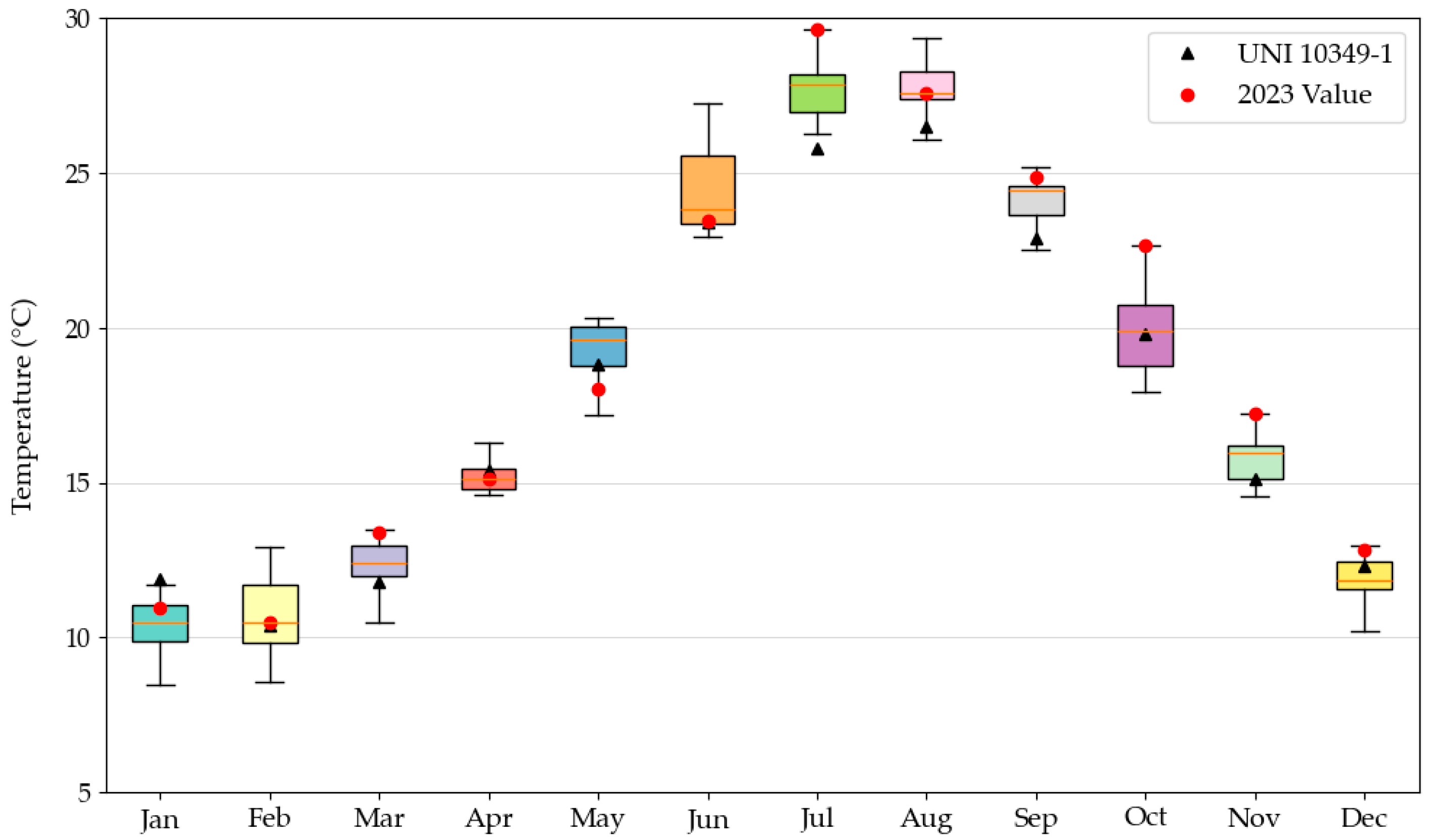
As already discussed, one of the reasons that justify the different outcomes between Blumatica Energy and the e-DSS is the use of different weather datasets. In order to remove the effect of weather data, a further test was conducted by forcing the data retrieved from UNI 10349-1:2016 (and used by Blumatica Energy) into the e-DSS.

In this case, the accordance between the heating needs in the current building configuration was highly improved; heat losses now differed by only 0.6%, while heat gains were still overestimated but only by 4.5%. Consequently, the heating demand calculated by the e-DSS was only 0.8% below the value obtained from Blumatica Energy. Similarly, in the cooling season, both heat gains and heat losses were slightly overestimated by the e-DSS, with an overall 2.5% difference in the cooling needs. However, and quite surprisingly, worse outcomes emerged in the simulation of the building after renovation; actually, in both seasons, the solar gains through the windows were strongly underestimated, leading to higher heating demand (+35.9%) and lower cooling demand (−36.7%) than in Blumatica Energy. The reason behind this outcome is discussed in Section 4.3.

4.3. Discussion and Possible Improvements of the e-DSS

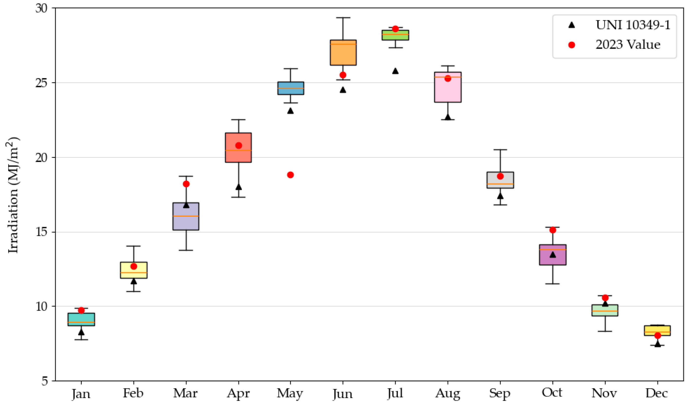
As outlined in the previous sections, the first important issue in the e-DSS is the choice of the weather data used to calculate the thermal energy demand. While Blumatica Energy adopts the official weather data available in the Italian standard UNI 10349-1:2016 [25], the e-DSS retrieves data from the online service PVGIS so that they can be available for every location worldwide. Moreover, the UNI data represent a long-term average, while PVGIS data correspond to a specific year (2023 in this case). This does not allow for direct comparison between the two tools but cannot be regarded as an error in the e-DSS; indeed, the main reason for using this tool is a quick and preliminary evaluation of the benefits ensured by e-SAFE renovation, which is still feasible. A more robust approach would require downloading and averaging several years of weather data from PVGIS, which is feasible but would made the tool cumbersome and slow down the simulations.

Another limitation of the e-DSS is that it does not allow for describing the presence of different types of windows, roller shutters, and movable shading devices. Moreover, the attribution of the projection factors in Table A4 is only associated with the presence of balconies and can assume a single value for each facade; instead, a real building can present other types of obstructions (vertical fins, opposite buildings), and the balconies in a certain facade can provide different shading patterns to the various windows. The error introduced by this limitation in the e-DSS depends on the specific building, but in principle, this is likely to bring about an underestimation of the shading effect, especially in the summer.

Two further main simplifications were identified that justify the discrepancies between the results from the e-DSS and Blumatica Energy, and both regard the calculation of the solar gains through the glazed components.

The first simplification consists of neglecting the “exposure factor” (F_w) introduced by UNI/TS 11300-1:2014; this multiplies the solar transmission factor (g_factor) to account for the incidence angle of the solar radiation against the glazed surface and depends on the orientation, the type of glazing, and the month. For instance, the “exposure factor” for a south-oriented double glazing ranges between 0.90 and 0.98 in the winter months, but it becomes 0.77 to 0.80 in the summer months. Instead, an east-oriented double glazing has F_w = 0.86 to 0.90 in the winter and F_w = 0.915 in the summer. Neglecting this term in the e-DSS obviously implies overestimating the solar gains.

The second simplification consists of using a constant shading factor (f_shade), which means assuming that the movable shading devices are always closed. In fact, UNI/TS 11300-1:2014 corrects this factor to consider that the shading device is closed over a certain percentage of time (t_with), while in the remaining time (1 − t_with), the shading device is open because the solar irradiance values are low:

$$f_{shade\_coor}=t_{with}·f_{shade}+\left(1-t_{with}\right)$$

(41)

Default values are available for t_with, according to the orientation and the month. For instance, a south-oriented shading device has t_with = 0.56 to 0.82 in the summer and t_with = 0.81 to 0.86 in the winter. North-facing shading devices always have t_with = 0, meaning that they are always open. Now, let us apply Equation (41) in July to a south-facing window (t_with = 0.62) both before renovation (f_shade = 0.8) and after renovation (f_shade = 0.35):

$$\mathrm{Before} \mathrm{renovation}: f_{shade\_coor}=0.62·0.8+\left(1-0.62\right)=0.876$$

(42)

$$\mathrm{After} \mathrm{renovation}: f_{shade\_coor}=0.62·0.35+\left(1-0.62\right)=0.597$$

(43)

From this example, it is possible to understand that the error caused by using a constant shading factor in the e-DSS amounts to around 10% before renovation (f_shade = 0.8 in the e-DSS and f_{shade_corr} = 0.876 in Blumatica Energy), but it exceeds 60% after renovation (f_shade = 0.35 in the e-DSS and f_{shade_corr} = 0.597 in Blumatica Energy). In both cases, the error leads to underestimating the solar gains in the e-DSS but to an unacceptable degree for the renovated building. This fully justifies the results presented in Section 4.2 and suggests that the two main simplifications discussed above should be avoided to provide a more reliable and realistic tool.

Finally, it is worth mentioning that the e-DSS has been tested by many technicians (mainly engineers and architects working either in construction companies or as freelance designers) during a series of dissemination and training activities conducted between 2022 and 2025 in Italy and Greece in the framework of the e-SAFE project. Around 40 participants were involved in the four events organized so far, and they were asked to simulate a residential building with the e-DSS, while also proposing and evaluating possible renovation solutions. The only data they were provided with were plans, perspective drawings and some information about wall assemblies, roofs, window types, and existing thermal systems.

During the final open discussion, almost all the participants expressed their satisfaction with the tool, highlighting its user-friendliness. In their opinion, no specific training is needed to use it, but on the contrary, its streamlined data input allow professionals to easily and quickly address a preliminary design stage. The technicians also provided suggestions for further improving the tool; the main recurrent suggestion regarded the possibility of implementing an algorithm to size the heat generators in the design stage, based on the building’s heat load, which is now left to user experience.

5. Conclusions

The findings presented herein suggest that the e-DSS can be used as a valuable and user-friendly tool for preliminary energy performance assessment of non-historical buildings with RC structural frames, before and after an e-SAFE renovation. Its primary function is to guide users in the decision-making process, thus helping in the choice of the most suitable energy-and-seismic renovation solution based on the features of the building. Its user-friendliness has been recognized by a pool of technicians (engineers, architects) involved in a series of training activities in Italy and Greece in the framework of the e-SAFE project. Apart from expressing their satisfaction, the technicians also provided suggestions for further improving the tool.

The e-DSS also highlights potential energy, cost, and environmental benefits. However, it is important to acknowledge that the e-DSS is neither intended for highly precise energy calculations nor for energy performance certification. The use of real weather data available from the freely accessible PVGIS service, while making the tool versatile and globally applicable, prevents direct comparison with other tools employing typical weather years. Nevertheless, it ensures a robust internal comparison between the pre- and post-renovation scenarios within the e-DSS framework. To further enhance its accuracy, future code improvements are necessary, particularly concerning the implementation of correction factors to simulate the operation of movable shading devices and the angle of incidence for solar radiation. Conversely, other simplifications within the code, such as those related to heat losses through thermal bridges and the projection factors for windows on balconied facades, introduce deviations that are deemed acceptable for preliminary assessments.

This initial study focused only on KPIs related to the energy performance of the building envelope. The simulation of thermal systems will be addressed in subsequent research. Moreover, the case study is a residential building located in a warm region of southern Italy. Future work should validate the e-DSS’s robustness across diverse climatic regions, potentially heating-dominated, and for other building typologies beyond residential applications. So far, the tool can be used only in Italy, Greece, and Romania, because for these countries, it includes a suitable database of materials, costs, and regulations.