Reduced-Order Model for Bearingless PMSMs in Hardware-in-the-Loop

Abstract

High production costs and extended development timelines pose significant challenges to the manufacturing of bearingless permanent magnet synchronous motors (BPMSMs). Moreover, uncertainties regarding the motor’s ability to generate suspension and torque often persist even after prototyping, primarily due to the limitations of lumped parameter models in capturing the system’s complex dynamics. Since this technology is not yet fully consolidated, there is a clear need for a solution that enables the effective evaluation of BPMSMs prior to physical production. To address this, a reduced-order model (ROM) was developed for BPMSMs with combined windings, capturing the cross-coupling effects associated with rotor eccentricity, magnetic saturation, and topological complexity. The model was constructed using the parametric interpolation method (PIM), enabling efficient and accurate representations of nonlinear electromechanical behavior as ferromagnetic materials and spatial harmonics are addressed through finite element modeling. Additionally, hardware-in-the-loop (HIL) techniques were used for gain tuning, and active disturbance rejection control (ADRC) was applied to enhance performance. This combined approach offers a comprehensive solution for the design and control of BPMSMs.

1. Introduction

This research addresses the challenge of enhancing suspension control in BPMSMs by developing and validating an ROM that captures the coupled electromechanical dynamics of the system, including radial force generation. The proposed ROM is constructed using the PIM, enabling efficient and accurate modeling of nonlinear behavior while maintaining computational tractability suitable for real-time applications. This study tackles several key challenges: (1) the formulation of a ROM that accurately represents the bearingless motor, capturing the coupled dynamics [1]; (2) the implementation of the model in discrete time to ensure compatibility with digital control systems; (3) the integration of inverter dynamics to improve model fidelity; and (4) the deployment of the ROM within a HIL simulation framework to validate and optimize control strategies, with a particular focus on ADRC.

The motivation for this work arises from the high cost, extended development timelines, and complexity associated with manufacturing physical prototypes of bearingless motors. By utilizing HIL simulation, it becomes possible to test and refine both control algorithms [2] and dynamic models in a real-time environment, significantly reducing development time, resource consumption, and risk during early-stage design.

Despite the increasing use of HIL techniques in power electronics and motor control, their application to BPMSMs, particularly for validating ROMs and advanced control strategies, remains limited. The existing literature has largely focused on magnetic bearings or full-order finite element models, which, while accurate, are computationally intensive and unsuitable for real-time control development [3]. Moreover, most prior studies assume dedicated suspension windings, where the electromechanical coupling is minimal and the modeling task is comparatively straightforward [4].

The central innovation of this work is the development of the first ROM specifically designed for BPMSMs with combined windings, as found in dual-purpose non-voltage (DPNV) configurations [5]. This topology introduces a coupling between suspension and torque generation, significantly increasing the complexity of the system’s dynamic behavior. To the best of the author’s knowledge, no prior work has proposed a dynamic ROM capable of capturing the coupled translational and rotational behavior inherent to this configuration. While motor and inverter topology, control strategies, and use of HIL techniques are relatively conventional and well-established in industrial practice, the modeling methodology introduced in this study is novel and represents a foundational contribution to the field.

By enabling accurate, real-time modeling of complex electromechanical interactions in BPMSMs with combined windings, this approach not only advances academic understanding but also provides a practical tool for engineers. It facilitates faster prototyping, reduces reliance on costly physical testing, and supports the development of more robust and adaptive control systems, ultimately accelerating the deployment of high-performance bearingless motor technologies in real-world applications.

The remainder of this paper is structured as follows. Section 2 and Section 3 review the fundamentals of BPMSMs and the development of the ROM. Section 4 presents the adopted control strategy. Section 5 details the HIL simulation results. Section 6 discusses the performance of the ADRC controller. Finally, Section 7 concludes this study and outlines directions for future research.

2. Bearingless PMSMs

The available bearingless motor technologies constitute a diverse range of designs, each leveraging unique electromagnetic principles to enable combined torque generation and levitation. These include surface-mounted permanent magnet motors, known for their high efficiency; homopolar motors, characterized by their distinctive flux distribution; consequent pole motors, offering simplified construction; induction motors, utilizing induced currents for operation; switched reluctance motors, relying on variable reluctance for torque production; and interior permanent magnet motors, which embed magnets within the rotor to enhance performance. The preference for surface-mounted permanent magnet motors is often driven by their superior efficiency and the applicability of magnetostatic solvers for accurate electromagnetic field analysis.

The geometry of the BPMSM used in this study was defined using RMxprt software (2023 R2), based on a comparative analysis of existing bearingless motor designs reported in the literature. Eight key design characteristics were identified and used as selection criteria, as summarized in

Table 1. Comparison between the bearingless PMSM designs.

Reference	[6]	[7]	[8]	[9]	[10]	[11]	[12]	[13]		Author Design
Rotor external diameter (mm)	65	39	33	24.5		29	200			73
Core length (mm)	80	45	40	50		75	100			65
Airgap (mm)	2	0.5	1	0.5	1	1				1
Stator external diameter (mm)	120	135	70	47.5	75	52				135
Power (W)	2.5 k	10 k		926	1 k		25.5 k	50 k		2 k
Suspension current (A)		25		2.47						2.5
Lateral force between the rotor and the stator (N)	8.7	280		128		470				85
Rotation (rpm)	10 k	100 k	60 k	4 k	60 k		30 k	25 k	100 k	3 k

. These characteristics include parameters such as rotor topology, stator slot configuration, winding type, and the suspension integration method. It is important to note that not all references provided complete information for every characteristic; however, the comparison was sufficient to guide the design process. The final column of Table 1 presents the configuration adopted in this work. A visual representation of the resulting rotor and stator geometry is provided in Figure 1.

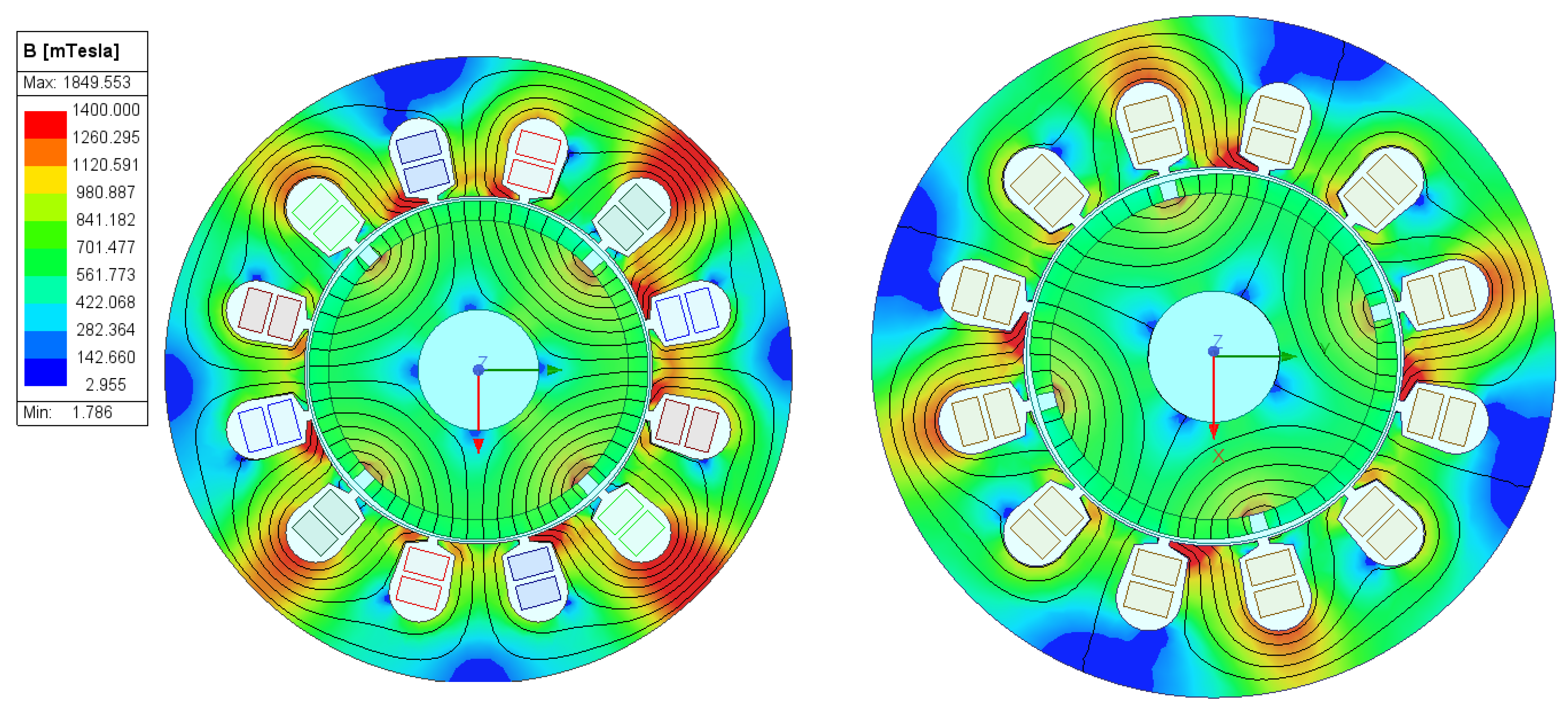
The analysis of magnetic flux involves evaluating the induction in the rotor and stator laminations, which is crucial for efficiency [14]. A common design criterion for magnetic flux is to avoid core saturation, as highly saturated machines lead to inefficient current usage, resulting in increased copper losses. Saturation can also cause undesirable effects, such as excessive vibrations, acoustic noise, overheating, and potential damage to machine components.

In high-performance electric machines, magnetic flux densities typically range from 1 to 1.5 Tesla, which are sufficient to achieve high efficiency and torque density, key attributes for applications such as electric vehicles, compressors, and other compact, high-power systems. For the motor proposed in this study, and excluding the contribution from the suspension control flux, the calculated flux density reached 1.87 Tesla. This value is strongly influenced by the magnetic properties of the core material. It is important to note that peak flux values may arise from geometric singularities, such as sharp tooth tips, or from discretization artifacts introduced by the finite element mesh. Given that peak flux was not a primary focus of this study, and considering the potential unreliability of such localized measurements, it is not considered a meaningful indicator of overall machine performance in this context.

2.1. Additional Motor Data

At a synchronous speed of 3000 rpm, the machine delivers an output power of 2001.3 W and a rated torque of 6.37 N·m. The root mean square phase and line currents are both 6.76 A, and the maximum line-induced voltage reaches 366.8 V. The electrical loading characteristics include an armature thermal load of 254.4 A²/mm³, a specific electric loading of 30.9 A/mm, and an armature current density of 8.21 A/mm². Losses are accounted for, with 12 W due to friction and windage, 18.5 W from iron core losses, and 205.261 W from armature copper losses, totaling 235.7 W. This results in an input power of 2237.0 W and an overall efficiency of 89.5%.

2.2. Dual-Purpose No-Voltage Winding (DPNV)

There are two main types of winding for bearingless motors: separated and combined. The separated winding has specific turns for torque and lateral force in the same stator slot. On the other hand, the combined winding uses the same winding and is also referred to as dual-purpose. The combined winding is superior in terms of thermal utilization and is simple to manufacture [6].

In the DPNV winding, there are two three-phase terminals, half for torque and half for suspension, but in the middle point of the coils. In terms of connection for the drive, there are some possible variations, such as parallel, bridge, and midpoint current injections. This bearingless connection was applied, in which it is possible to apply a smaller inverter for suspension in comparison to the motor.

For a more comprehensive understanding of this winding method, Severson provides a detailed explanation of its design principles in [5,15] and discusses its practical implementation in [16]. The winding diagram of the selected motor is in Figure 2.

Evaluation of the Suspension Forces

Unlike conventional motors that rely on mechanical bearings, BPMSMs achieve contactless rotor suspension by generating active radial forces through controlled magnetic fields. The suspension forces are produced by intentionally creating asymmetric magnetic fields in the airgap. When the rotor is displaced from the center, the control system detects this deviation and adjusts the suspension current to generate a restoring force.

The electromagnetic behavior of the bearingless PMSM is governed by the interaction between stator currents and the magnetic field in the airgap. These forces were modeled using ANSYS Maxwell (2023 R2), a finite element analysis tool, ensuring that the simulation results are physically accurate and consistent with analytical formulations. The torque and radial suspension forces are derived from Maxwell’s stress tensor and flux linkage principles in Equation (1):

$$T_e={\displaystyle \frac{3}{2}}p({\psi }_d{i}_q-{\psi }_q{i}_d)$$

(1)

where $T_e$ is the electromagnetic torque, $p$ is the number of pole pairs, ${\psi }_d$, ${\psi }_q$ are the d- and q-axis flux linkages, and $i_d$, $i_q$ are the d- and q-axis currents.

The radial suspension forces in the X and Y directions can be approximated in two forms by an integral or in a simplified linearized form, as shown in Equation (2):

$$F_{x,y}={\displaystyle \frac{1}{{\mu }_0}}{\int }_S\left(B_n^2-B_t^2\right) dS \mathrm{or} F=k\ast e$$

(2)

where $B_n$ and $B_t$ are the normal and tangential components of the magnetic flux density, ${\mu }_0$ is the permeability of free space, $S$ is the surface area over which the stress is integrated, $k$ is the stiffness coefficient, and $e$ is the rotor displacement from the center.

These equations form the basis for the ROM, which maps a high-dimensional input space (currents, rotor position, and eccentricity) to outputs, including torque and radial forces.

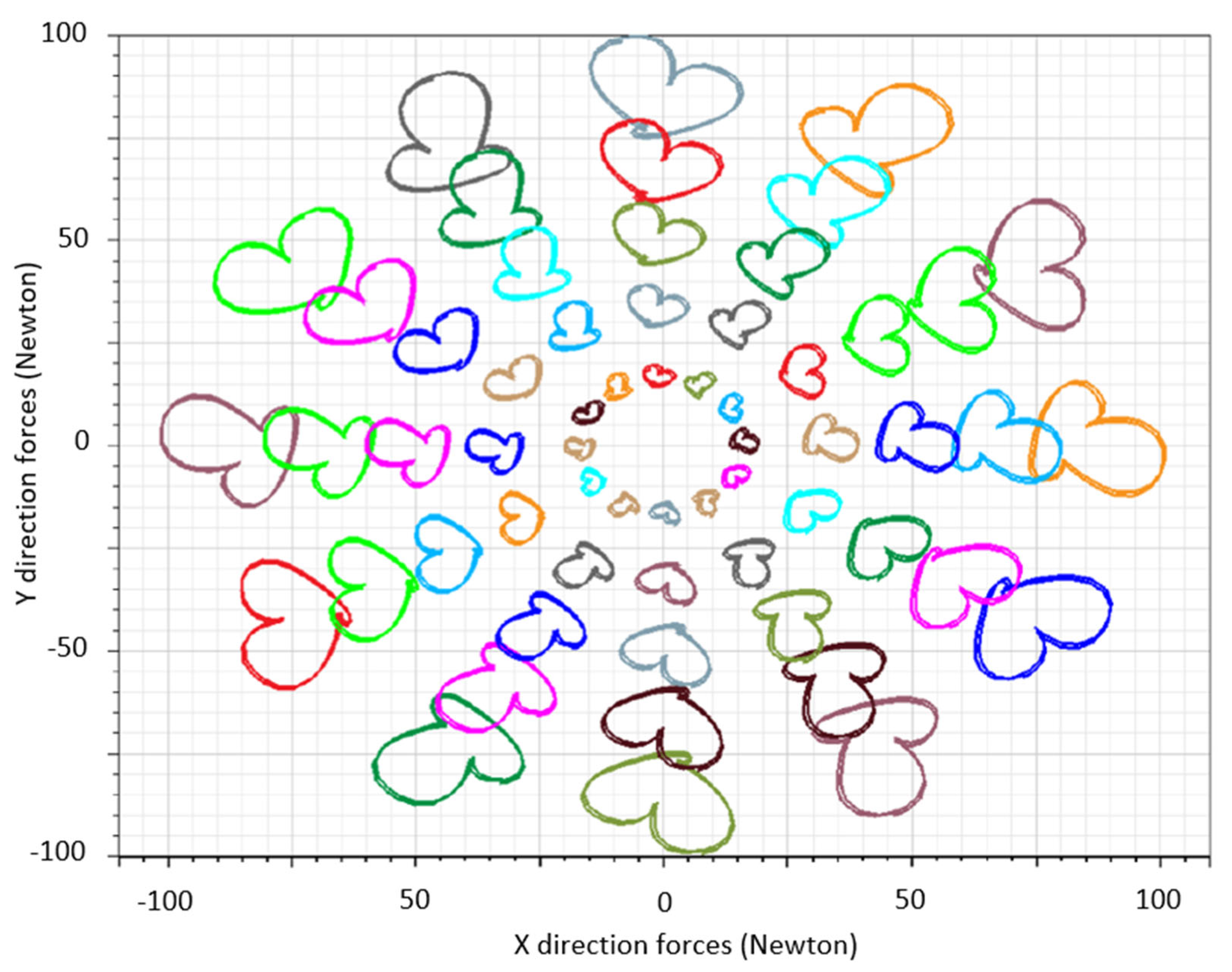
The force diagram in Figure 3, plotted at 30° electrical angle intervals, demonstrates that the bearingless system can generate uniform force in all directions using five suspension current steps. This confirms that adjusting suspension current amplitude and electrical angle allows rotor movement relative to the stator. As the suspension forces increase, the deviation increases as well proportional to the suspension current. In Figure 3, a maximum suspension force of 100 N is achievable; however, a variation of up to 25 N is observed. This increasing variation is visually represented by the expansion of the heart-shaped contour, indicating a growing asymmetry in the force distribution.

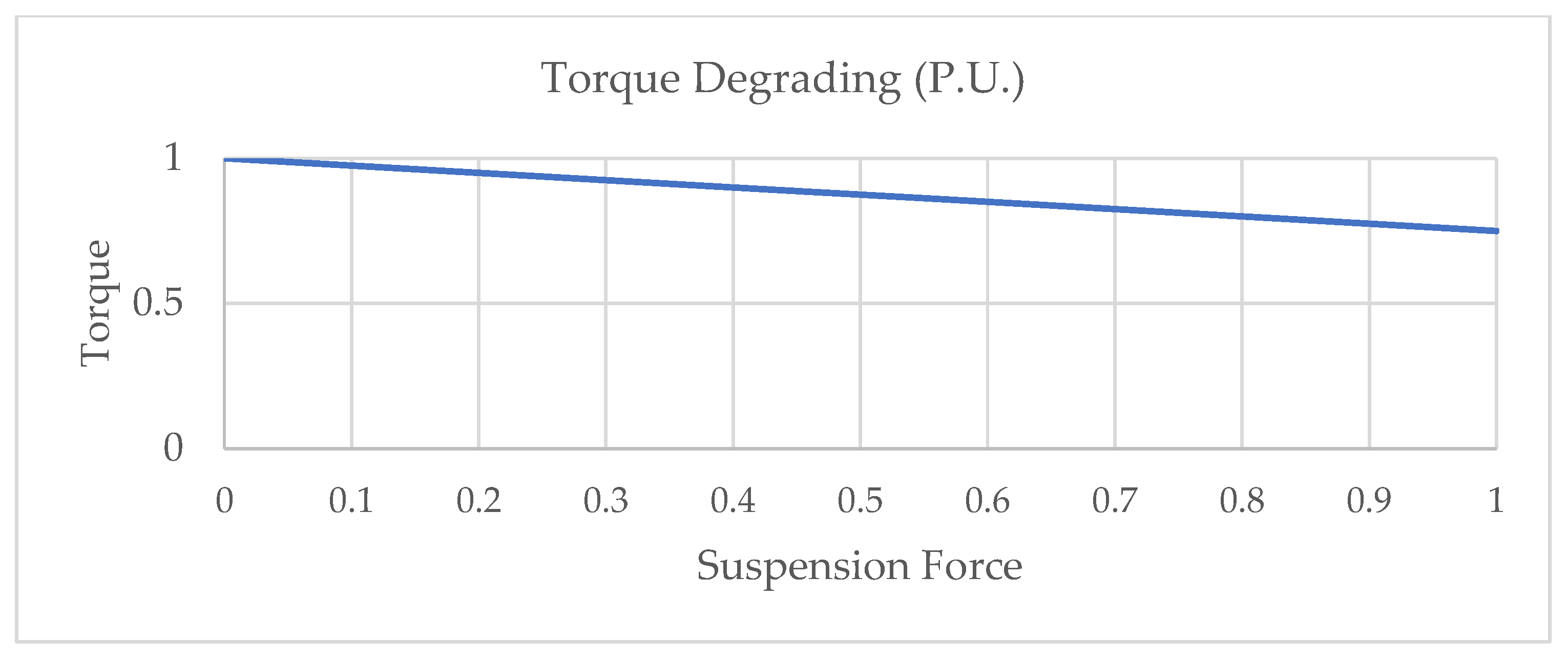
Figure 4 illustrates how increasing the suspension force leads to a linear reduction in normalized torque output (P.U.). As the suspension force rises from 0.0 to 1.0, the torque decreases from 1.0 to approximately 0.75, highlighting the trade-off between force generation and torque performance in the bearingless motor.

3. Reduced-Order Model

Reduced-order modeling techniques provide an approach to simplify complex systems while preserving their essential dynamics, enabling faster simulations and control design [17,18]. This approach is particularly advantageous when dealing with intricate systems that require real-time performance or rapid prototyping. Bearingless motors, which integrate both motor and magnetic bearing functionalities, present unique challenges due to their inherent complexity and strong coupling between different physical domains [19].

Traditional control design approaches often rely on lumped parameter models, which may overlook critical aspects of motor behavior, such as spatial harmonics and material nonlinearities. Similarly, conventional ROM generation techniques, such as flux tables, are typically tailored for standard three-phase motors with fixed, centered rotors, making them unsuitable for bearingless motor applications. To address these limitations, this study introduces the first ROM for a BPMSM using the PIM approach. Unlike previous works [20,21,22,23], which focused on reluctance motors and employed proper orthogonal decomposition with interpolation, the methodology presented here offers a novel and more adaptable solution tailored to the unique dynamics of bearingless systems.

3.1. ROM Development for Bearingless Motors

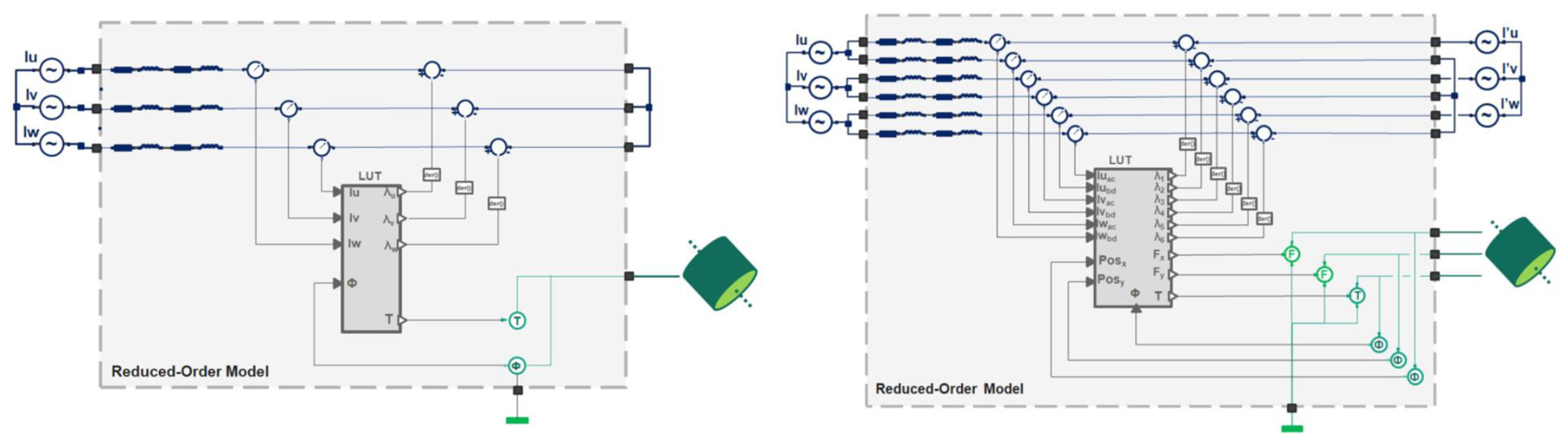
The selection of appropriate input and output variables is paramount, as these determine the scope and fidelity of the ROM [24]. The procedure to obtain the ROM is explained and has three main steps: (1) the conventional motor (left side of Figure 5), (2) an evaluation with no eccentricity to obtain the equation forces in the horizontal and vertical directions, and (3) the eccentricity (right side of Figure 5). For further details, [1] can be checked. This brief procedure will be explained in the next two paragraphs.

In the first step, the generation of the ROM often involves a full factorial sweep table, exemplified by a model with 3000 points derived from a 5³ × 24 configuration, considering three phase currents, the electrical angle, and torque.

In contrast, a BPMSM, particularly one with a DPNV winding configuration, introduces significant complexity to the ROM. Such a motor incorporates three phases for torque generation, along with voltage injection at the midpoint of the coils, resulting in the escalation of input parameters to nine, encompassing positions in the X and Y directions, and the outputs expand to include forces in both directions in addition to torque.

The computational demand to generate a comprehensive ROM for the bearingless motor far exceeds conventional software capabilities, potentially requiring approximately one week of processing time even with software modifications; a full factorial model, also known as a full space model, for this system involves a sweep table with 1,000,000 points (5⁶ × 2² × 16), highlighting the substantial increase in complexity compared to a three-phase ROM motor.

In the second step, to enable ROM creation, lateral rotor displacement is suppressed, and the rotor operates without eccentricity, while suspension forces are generated via a voltage applied to the suspension terminals, streamlining the model. The process involves selecting five current sweep steps for each phase, optimizing the balance between computational efficiency and model fidelity. The obtention of the correction factor for the horizontal and vertical directions was explained by [1], and the values are 479.300 and 478.500 Newtons per meter, respectively.

3.2. ROM Validation

The third and last step, the transient finite element simulation, is used to accurately represent the bearingless motor’s condition and serves as a benchmark for validating the reduced-order model. This validation involves comparing torque, current, and force outputs between the reduced-order model and the finite element simulation to ensure that the simplified model reliably captures the system’s dynamic behavior. The average error was below 3% for torque and 5% for radial forces, confirming the ROM’s fidelity.

4. Control

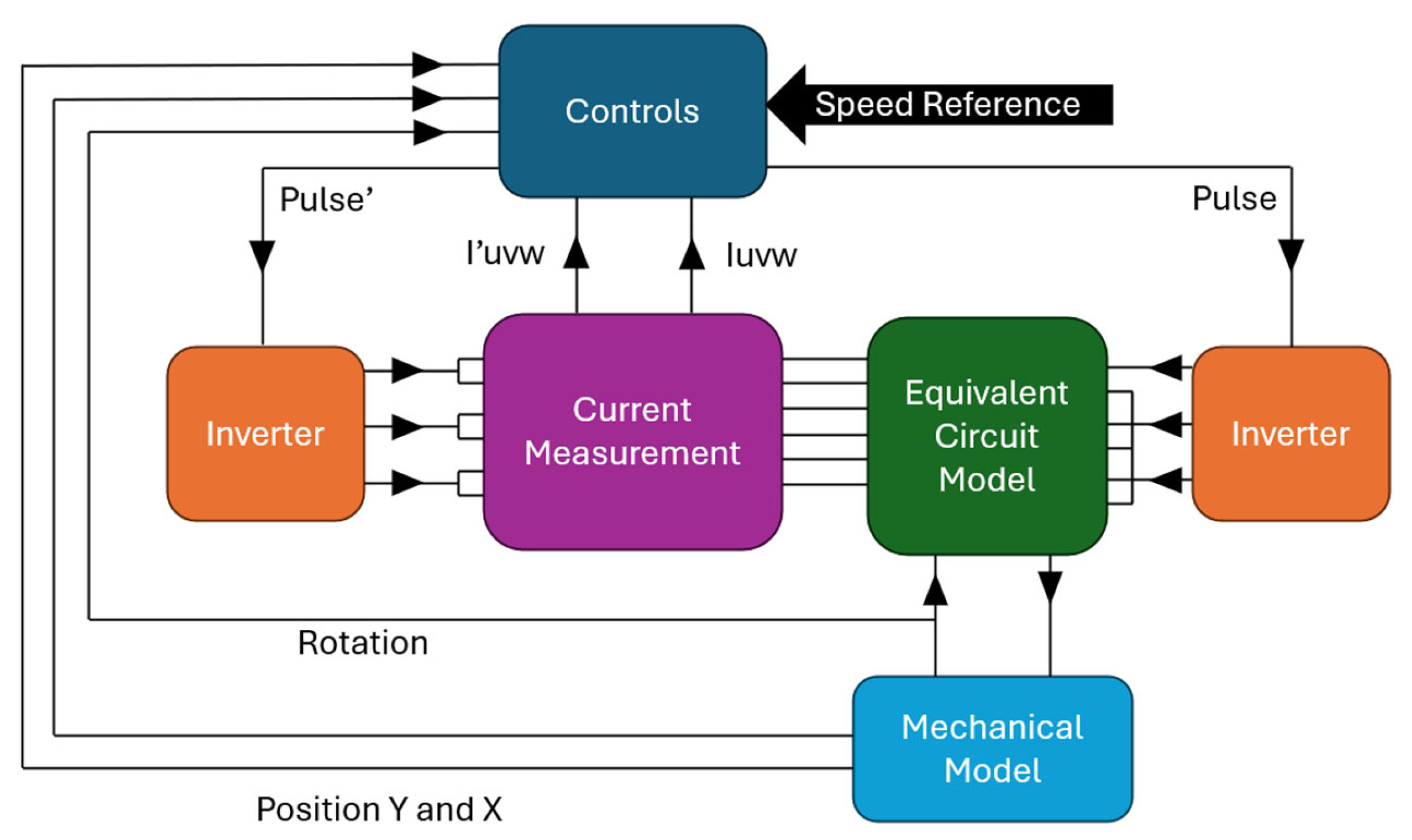
The strategy adopted for the bearingless PMSM control will be explained in this section. Figure 6 presents the configuration of blocks composed of the control, current measurements, the equivalent circuit model, the mechanical model, and inverters. The external input data are the speed references in the control block, as detailed in Figure 7. The control block is composed of the torque and suspension control. The internal inputs are positions X and Y, the rotation, and currents for the torque and suspension. The output is the currents for both inverters. The target is to keep the rotor at the center position of the stator and track the speed reference. All blocks will be explained in detail, except for the inverter block and the current measurement, which are considered less relevant.

The field-oriented control (FOC) torque current loop and suspension loop, illustrated in Figure 7, will be discussed in Section 4.1 and Section 4.2, respectively. The current uvw to αβ block is shown in Section 4.4. The SVPWM generator block produces the switching signals for the PWM converters using the space vector pulse with modulation technique, with a switching frequency of 8000 Hz.

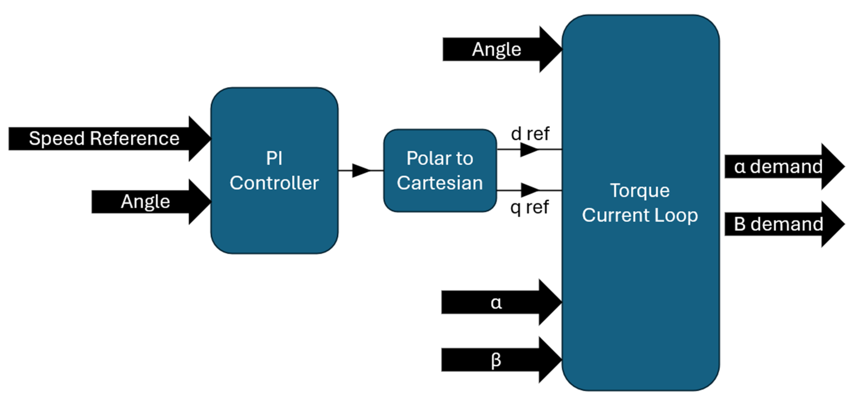
4.1. Torque Control

The implementation of torque control in conventional three-phase motors or advanced bearingless motors often utilizes an FOC strategy that employs a proportional-integral (PI) controller [25]. This control approach relies on the precise measurement of the rotor speed and phase currents, which are then transformed into the DQ reference frame to enable a direct comparison against reference DQ values. The torque control method combines proportional and integral controllers with field orientation control, making it applicable to both traditional three-phase motors and bearingless motors [25].

The fundamental principle involves continuously monitoring the rotor speed and phase currents, converting them into DQ components, and comparing them to reference values. Any discrepancy between the measured and reference DQ values triggers an adjustment in the current magnitude, either increasing or decreasing it to minimize the error and maintain the desired operating conditions [19]. The PI controller’s alteration of the current aims to minimize the divergence between the actual and desired current values, thereby influencing the motor’s torque and, consequently, its rotational speed [26]. To achieve rotor position and speed management in a bearingless PMSM, a decoupling algorithm is required for the independent regulation of radial suspension forces and torque forces [27].

Figure 8 represent the torque control, and the internal loop is shown in Figure 9.

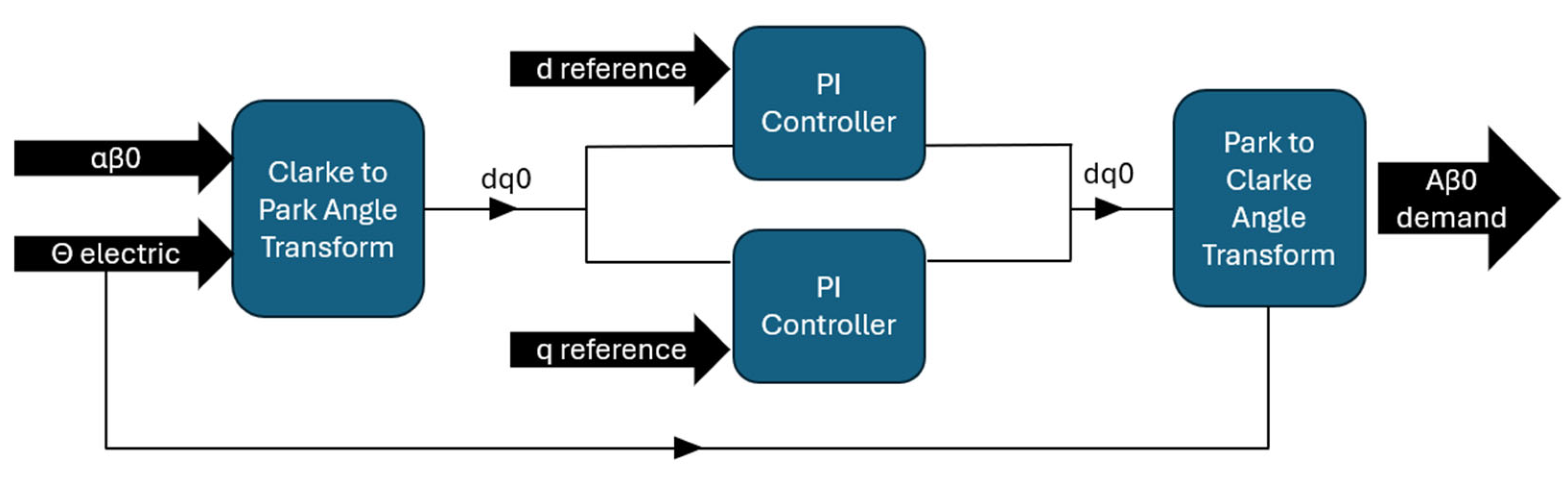
The implementation of FOC typically involves several key steps [19]. First, the motor currents are measured and transformed into a rotating reference frame, often the DQ frame, aligned with the rotor flux. This transformation decouples the flux and torque components of the current. Subsequently, PI controllers regulate the D- and Q-axis currents independently, providing precise control over flux and torque. The controller outputs are then transformed back to the stationary reference frame to generate the required stator voltages. Finally, pulse width modulation techniques are employed to synthesize these voltages and apply them to the motor windings [28].

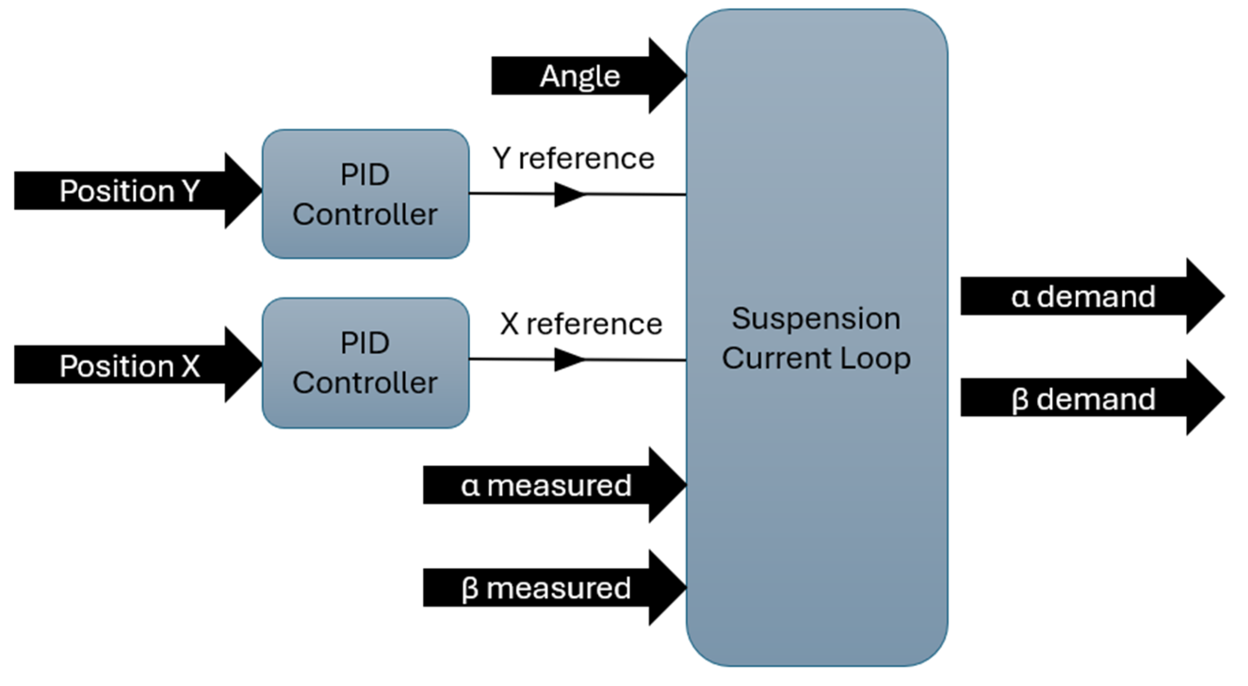
4.2. Suspension Control

The implementation of proportional–integral–derivative (PID) controllers in FOC systems necessitates careful consideration due to the inherent complexity of motor dynamics and the performance requirements of the drive system. Factors such as controller structure, process degree, the ratio of system time to process dead time, filter type and parameter setting, and nonlinear behavior influence the controller’s performance [29].

The structure of the FOC control is adapted to the suspension control, as shown in Figure 10. In addition, it is important to clarify that PI and PID controllers operate based on two primary inputs: the reference signal and the measured output. These are often combined into a single error signal, defined as the difference between the reference and the measurement. In the control architecture presented in this work, the outputs of the PID controllers correspond to current references. The DQ reference is different in comparison to the regular control, and it does not use the rotor or stator as a reference. The reference position is in the opposite direction of the rotor to obtain a stationary force in a rotating system. Suspension control requires a relatively high derivative gain, requiring extremely fast control. A different torque control is PI, and the suspension control is PID.

In contemporary motor control systems, the integration of PID control, in conjunction with FOC strategies, constitutes a cornerstone for achieving high-performance drive capabilities, providing a robust and versatile approach [30]. FOC, also referred to as vector control, endeavors to independently govern the flux and torque components of the motor current, thereby emulating the behavior of a separately excited DC motor [27]. This decoupling is typically realized through coordinate transformations, such as the Park and Clarke transformations, which project the three-phase stator currents onto a rotating reference frame aligned with the rotor flux [31]. Within this framework, PID controllers assume a pivotal role in regulating these decoupled current components, ensuring precise and rapid tracking of reference values [32]. The PID controller, encompassing proportional, integral, and derivative terms, offers a mechanism to minimize the error between the desired and actual values of controlled variables, such as torque and flux, by adjusting the motor’s voltage or current input. The proportional term delivers immediate correction based on the current error, while the integral term eliminates steady-state errors by accumulating past errors over time, and the derivative term anticipates future errors by considering the rate of change of the error signal [33]. A meticulously tuned PID controller, or a combination of multiple PID controllers, enhances the transient response, diminishes overshoot, and ensures the stability of the FOC system [34].

Internal Suspension Current Loop

This discussion about the internal loop, illustrated in Figure 11, is necessary due to the proposed improvement in control response, which will be presented in Section 6.

To mitigate external disturbances such as self-weight or vibrations that displace a rotor from its intended position, denoted as “y”, a control system employing an electromechanical actuator can be implemented. If an ideal linear actuator capable of instantaneously applying the required force along the “y” axis was available, the control strategy would involve measuring the displacement in “y” and commanding an opposing force from the actuator. This negative feedback mechanism would drive the position back to the zero point, contingent upon the closed-loop stability of the system. However, in real-world electromechanical actuators, force and current exhibit a strong correlation, often simplified to a direct equivalence, where force is proportional to current [35].

Given the absence of ideal current sources in physical systems, current flow necessitates the application of voltage. The relationship between voltage and current is governed by a dynamic transfer function. Consequently, to generate a specific current, the deviation between the desired current and the measured current must be determined, and a voltage proportional to this error is applied. This error-driven voltage application emulates an “ideal current source” from the perspective of the outer control loops. Therefore, an internal current loop is employed to calculate the voltage required to produce the desired current instantaneously. The outer suspension loop, in turn, determines the current necessary to achieve the correct position. Electrical dynamics are the fastest and most challenging to control.

Considering the control problem described, an FOC strategy is employed for the internal current loop within a suspension control system [19]. FOC, also known as vector control, offers a method to control AC motors in a manner analogous to DC motors [36]. This decoupling of torque and flux control enhances the dynamic performance of the motor drive. In this architecture, a PID controller is used in the outer suspension loop, while a PI controller is used in the inner current loop [37]. The PID controller in the outer loop provides precise suspension control, while the PI controller in the inner loop ensures accurate and rapid current regulation, which is crucial for achieving the desired force output. The current loop design directly impacts the motor’s dynamic performance and disturbance rejection, influencing current fluctuations, torque ripple, and system stability, especially under variable loads [38]. To stabilize the current control loop in high-speed regions, a novel configuration may be needed, where the current regulator connects to the conventional motor model in series [37].

4.3. Mechanical Model

As Figure 12 shows, the mechanical model is responsible for transforming the electrical torque into rotation and positioning the rotor according to the horizontal and vertical forces imposed by the control block.

The mechanical model of rotation presented in Figure 12 is simple. The electric torque acts, moving the rotor’s inertia and resulting in rotation, which is captured by the angle change along the time.

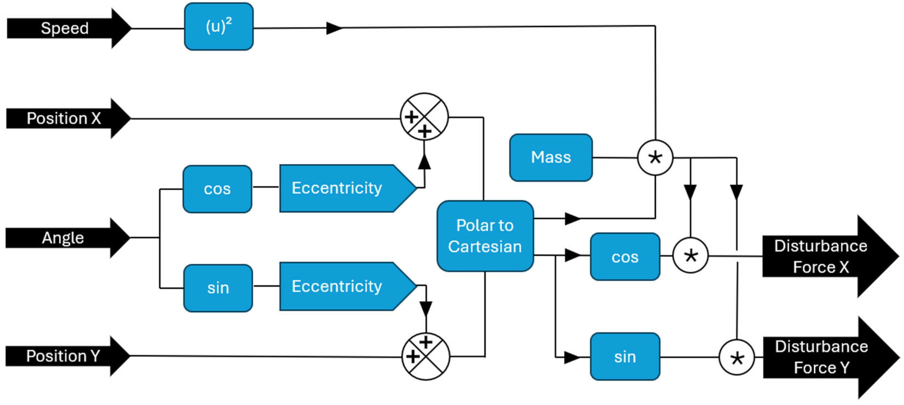
On the other hand, in Figure 12, the mechanical model of translation is complex. In the brief assessment, this block is responsible for the lateral movement of the rotor in relation to the stator in which the forces act on the position. Figure 13 presents the inner part of the mechanical model of translation, where the disturbance model is presented. There are disturbance forces in the horizontal and vertical directions, where the main difference is the weight of the forces in the vertical direction.

The function of the disturbance model is explained in Figure 14; basically, this block is ruled by Equation (3) for the unbalanced force:

$$U=m\ast e$$

(3)

where $U$ is the unbalanced force in g.mm; $m$ is the mass in grams; and $e$ is the eccentricity in millimeters.

To obtain the unbalanced force, the imbalance should be applied in Equation (4). As can be seen in Figure 14, there is no specific input for the imbalance, but it uses eccentricity, being the “e” of Equation (3). There is a direct correlation between imbalance and eccentricity, and the imbalance could be specified in terms of micrometers.

$$F=U\ast {\omega }^2$$

(4)

where $F$ is the unbalanced force in Newtons, $U$ is the imbalance in g.mm, and $\omega$ is the angular velocity in radians per second.

Disturbance

This is a deeper discussion of the disturbance or the selection of the unbalance. The eccentricity could be obtained through the recommendations of ISO 20940-11, which is applicable to mechanical vibration and rotor balancing, specifically on procedures and tolerances for rotors with rigid behavior.

According to Table 1 of ISO 21940-11 [39], the balance quality grade (G) for electric motors and generators with a shaft height of at least 80 mm should be 2.5, which is equivalent to 2.5 μm. Some standards, such as API 541 [40] applied to petroleum industries, required an even better balancing grade, such as 0.66. Considering the fact that bearingless motors are not mentioned in ISO 21940-11, it is recommended that the balancing grade be a maximum of 1.0 to reduce the disturbance and consecutively reduce the vibration and noise, but mainly the suspension current and energy.

For this experiment, 300 μm was employed as the eccentricity to explore the capacity of rejection disturbing. This level of unbalance is not appropriate for bearingless motors and is conventionally applied to crankshaft drives that are inherently unbalanced or rigidly mounted [39].

4.4. Equivalent Circuit Model

The equivalent circuit model is composed of several subsystems that demand a great number of figures for a deep explanation, but these are not relevant to the objective of this paper.

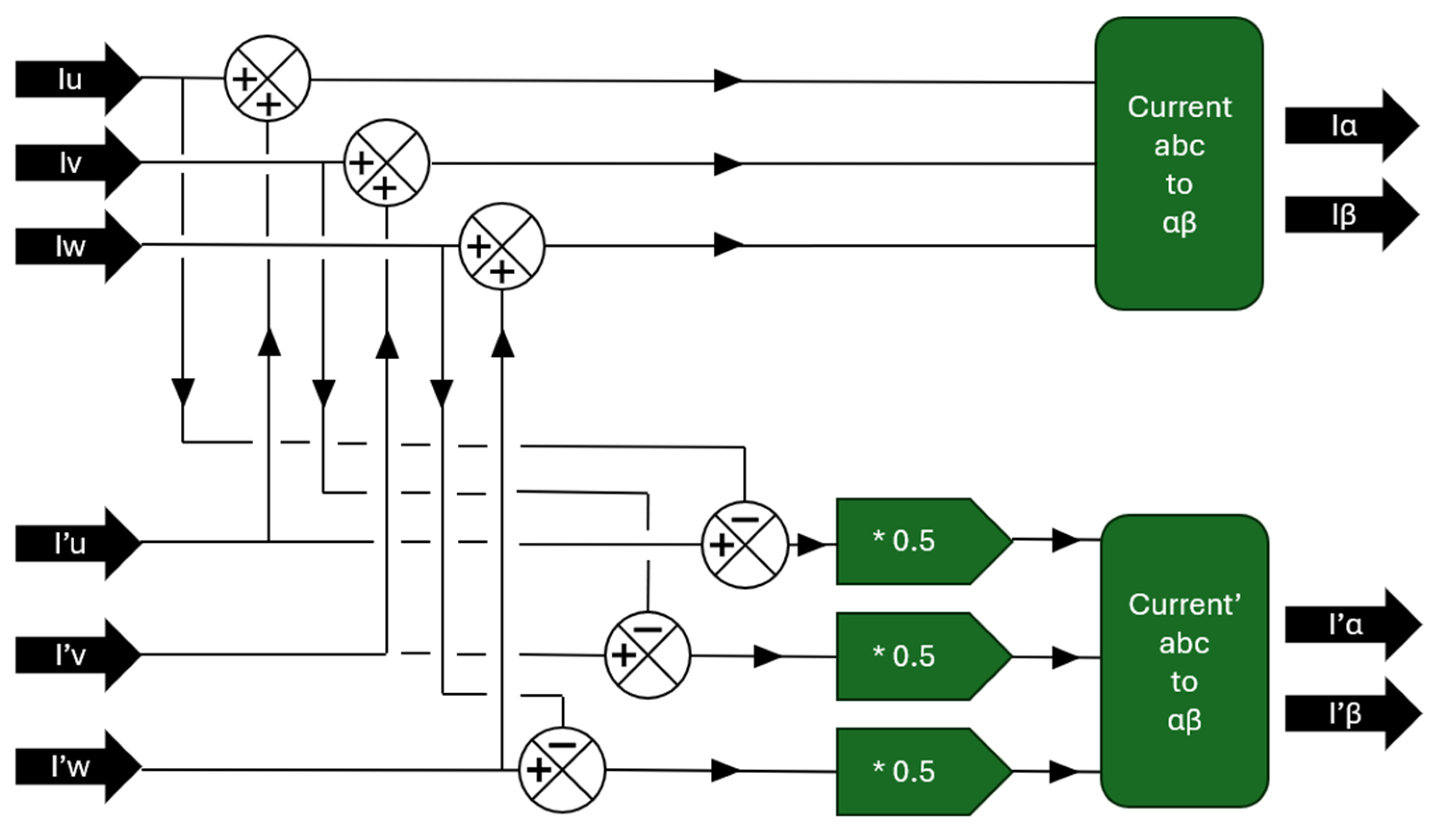
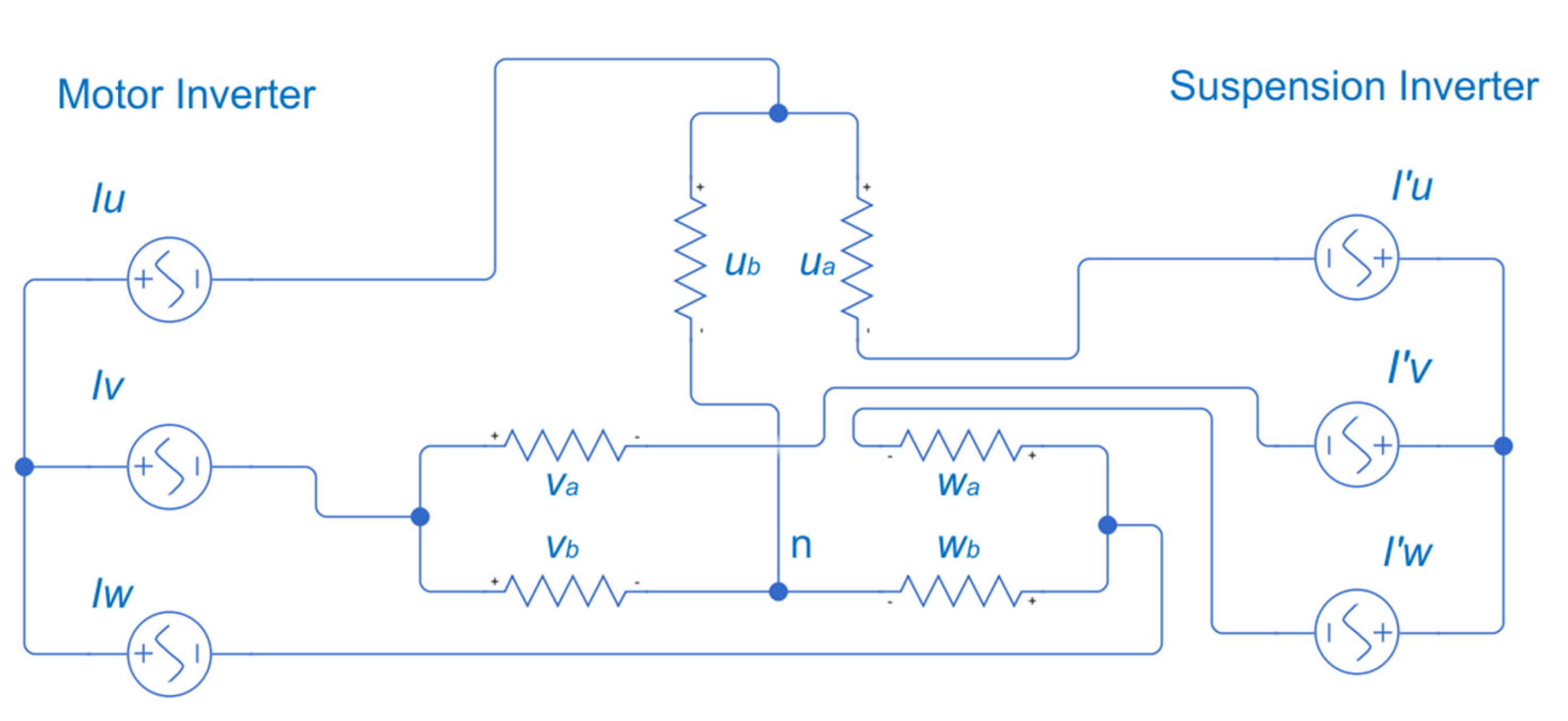
As it is necessary, an explanation of the method for obtaining the currents applied to torque and suspension is provided. Figure 15 presents six currents. The upper part is the current of torque, and the lower part, identified by the apostrophe, is the suspension current. As an example, Equation (5) presents the current of phase U as ${\overrightarrow{i}}_u$ for torque purposes, and Equation (6) presents ${\overrightarrow{i^{\prime }}}_u$ for suspension purposes, based on Figure 16.

$${\overrightarrow{i}}_u={\overrightarrow{i}}_a+{\overrightarrow{i}}_b$$

(5)

$${\overrightarrow{i^{\prime }}}_u={\displaystyle \frac{{\overrightarrow{i}}_b-{\overrightarrow{i}}_a}{2}}$$

(6)

Now, Equations (7) and (8) are shown in terms of ${\overrightarrow{i}}_a$ and ${\overrightarrow{i}}_b$, according to Figure 16.

$${\overrightarrow{i}}_a={\displaystyle \frac{1}{2}} {\overrightarrow{i}}_u-{\overrightarrow{i^{\prime }}}_u$$

(7)

$${\overrightarrow{i}}_b={\displaystyle \frac{1}{2}} {\overrightarrow{i}}_u+{\overrightarrow{i^{\prime }}}_u$$

(8)

A similar set of equations is listed by Torres [41], in which they evaluated the resonant control for DPNV winding applied to bearingless motors.

Figure 15. Summation to obtain currents for rotation and suspension. The symbols ‘+’ and ‘−’ represent addition and subtraction, respectively, indicating that values are summed or subtracted. The symbol ‘*’ denotes multiplication.

Figure 15. Summation to obtain currents for rotation and suspension. The symbols ‘+’ and ‘−’ represent addition and subtraction, respectively, indicating that values are summed or subtracted. The symbol ‘*’ denotes multiplication.

Figure 16. Connection in parallel for DPNV winding.

Figure 16. Connection in parallel for DPNV winding.

4.5. Results

The assessment of speed reference tracking performance is essential in evaluating the efficacy of motor control systems, particularly in applications demanding precise rotational speed regulation. In this context, Figure 17 illustrates the speed-tracking capabilities of the investigated motor drive system under dynamic operating conditions.

The motor, initially at rest, submits to a controlled acceleration phase, aiming to reach a speed of 1500 rpm within the first 0.35 s, which represents the first plateau of the speed. Then, the motor is commanded to accelerate further, targeting 3000 rpm just before 0.85 s, defining the second plateau, after which the motor maintains a steady-state operation at this speed until 1.25 s.

The performance of the torque control system is visually evident as the measured rotation speed, depicted in blue, closely tracks the speed reference trajectory, shown by the yellow dashed line. This observation highlights the effectiveness of the control algorithm in accurately following the desired speed profile, indicative of a robust and well-tuned control system. The maximum speed reached was 3006 rpm at 0.869 s, as well as a steady speed of 3001 rpm at 1.19 s, as illustrated in Figure 18.

The analysis of rotor dynamics involves a detailed examination of the rotor’s position and its orbital trajectory, providing crucial insights into the system’s stability and performance. Specifically, the position of the rotor is shown in Figure 19, where the red color represents the vertical direction in which the rotor starts the evaluation, being supported by the touchdown bearing. The blue color represents the horizontal direction; the readings of both directions are presented in

Table 2. Comparison between models summarizing the performance metrics of the PI and ADRC controllers. It highlights ADRC’s superior disturbance rejection and dynamic response.

	Condition 3000 rpm
Shaft Displacement (μm Peak to Peak)	SIMPLORER Ideal Source Continuous Time	Simplorer Inverter Discrete Time	SIMULINK	HIL PI Not Stable	HIL ADRC Stable	Improvement
Horizontal (X)	18	31	85	175 (200 spikes)	80 (no spikes)	54%
Vertical (Y)	18	45	114	160 (200 spikes)	80 (no spikes)	50%

.

The plot is a composition of X and Y positions, creating the orbit of the rotor along with time. Around the end (1.0 s), the orbit is stable.

Figure 20 shows the torque output to keep the speed as a reference. The load applied to the rotor is inertial according to the mass of the rotor. The torque is higher in comparison to the reference during the increase but is reduced to a plateau at a steady or constant speed.

The dynamic analysis of torque in a PMSM over time necessitates a comprehensive approach, considering various operational and design parameters that influence its behavior. Understanding torque production involves analyzing the complex interaction between stator and rotor magnetic fields, along with the motor’s electrical and mechanical characteristics. In Figure 20, it is possible to observe an increase in torque deviation between 1500 and 3000 rpm. For 1500 rpm, the maximum and minimum torques are 2.91 and 1.87 Nm, respectively, with an oscillation torque of 1.04 Nm. On the other hand, for 3000 rpm, the maximum and minimum torques are 5.52 and 4.01 Nm, respectively. At the rated speed, the oscillation torque is 50% higher, with a variation of 1.51 Nm. This is attributed to airgap eccentricity, a common imperfection in PMSMs that can indeed exert a significant influence on torque oscillations [42]. The magnitude of these torque oscillations is directly proportional to the severity of the eccentricity and the operating conditions of the motor. The torque oscillations induced by airgap eccentricity can have detrimental effects on the performance and lifespan, leading to increased noise and vibrations, reduced efficiency, the accelerated wear of mechanical components, and, in extreme cases, rubbing of the rotor against the stator [43].

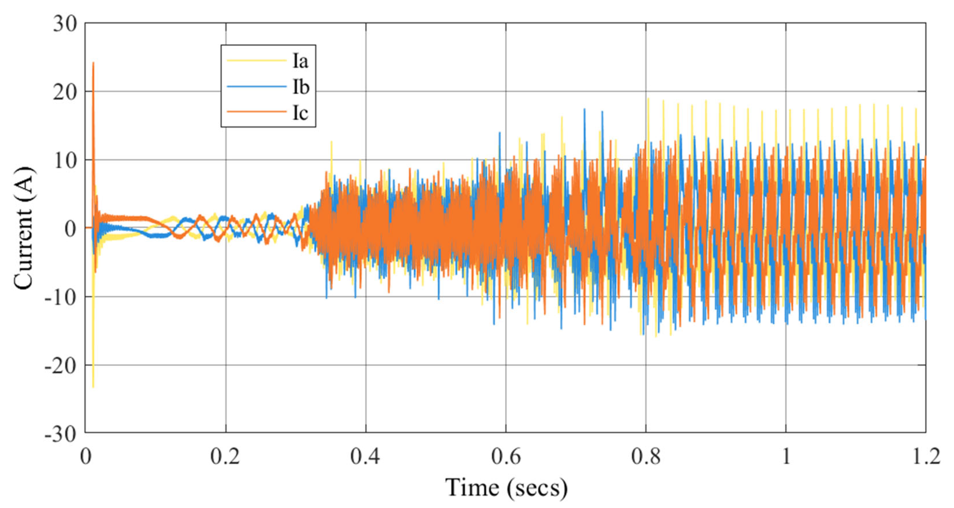
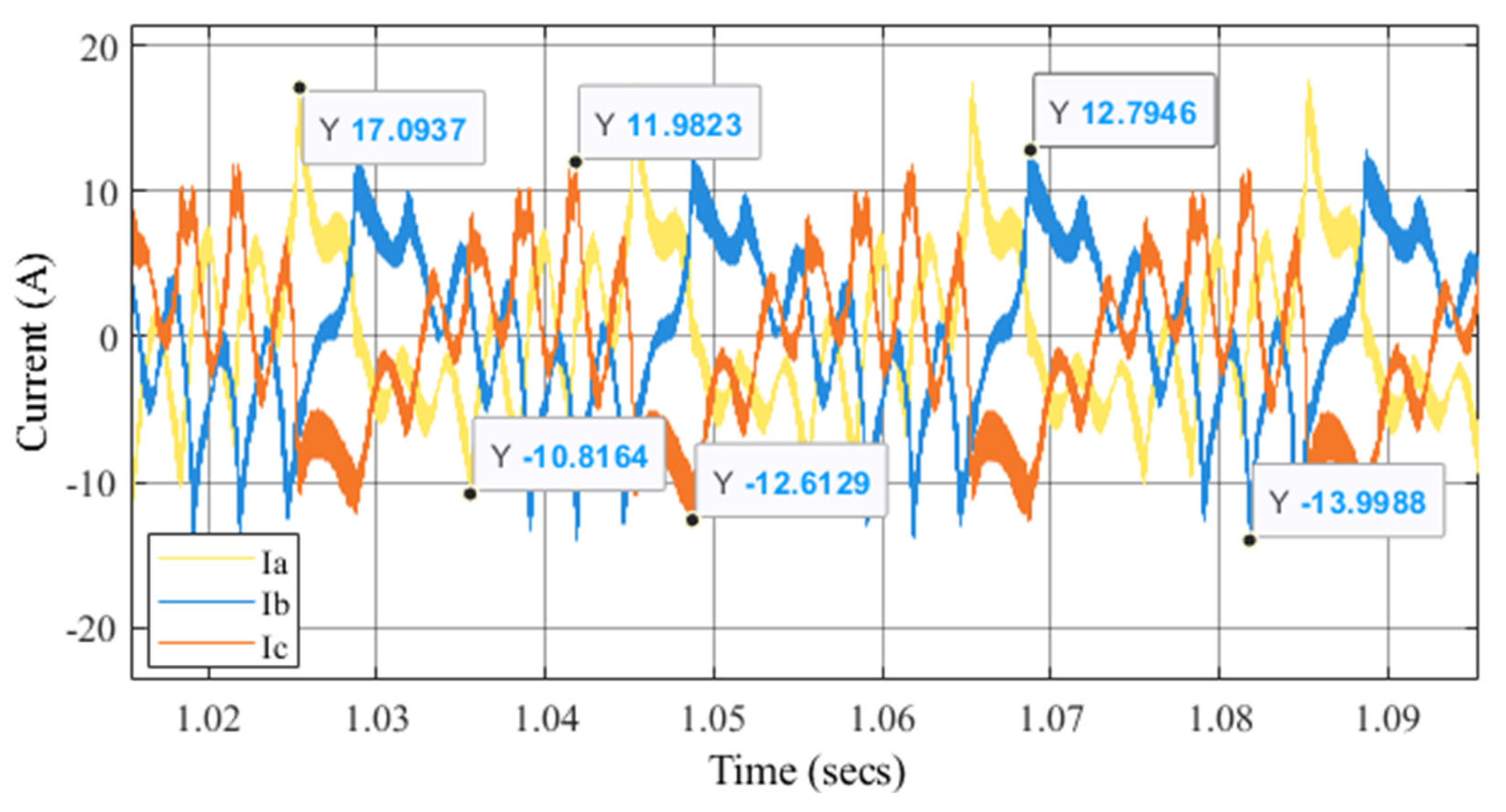
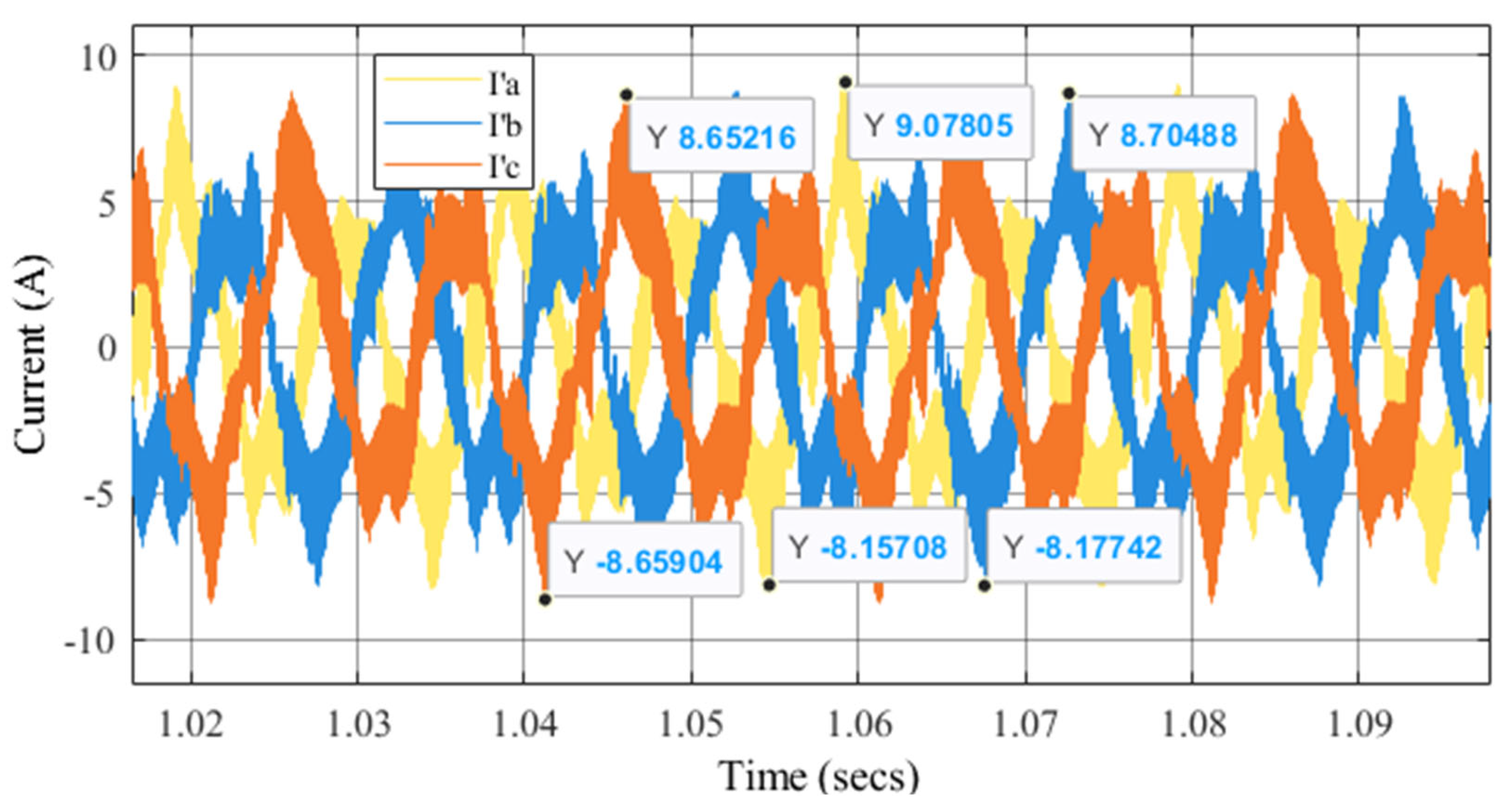
The waveforms of the winding currents related to the electromagnetic torque are shown in Figure 21. According to Figure 22, the peak-to-peak torque currents at 3000 rpm are 27.9 A, 26.8 A, and 24.6 A for phases a, b, and c, respectively. The current waveforms for the suspension winding are shown in Figure 23. For the suspension currents, shown in Figure 24, the values are 17.2 A, 16.9 A, and 17.3 A. These suspension currents represent approximately 63% of the torque currents.

The torque waveforms in Figure 21 indicate substantial current injections to drive mechanical output. However, slight amplitude differences among the phases (Ia, Ib, and Ic) suggest a degree of phase imbalance. Additionally, the waveforms deviate from perfect sinusoidal shapes, hinting at the presence of harmonic distortion. This distortion may stem from nonlinearities in the inverter and the influence of the suspension current, all of which can contribute to torque ripple. The implications of such characteristics include increased electrical losses, mechanical vibration, and acoustic noise, while the imbalance may reduce overall efficiency and impose greater thermal stress on the motor windings.

Figure 24 represents the suspension waveforms exhibiting significantly lower amplitudes and demonstrating a high degree of symmetry and balance across the three phases. Unlike the torque currents, the suspension currents are nearly ideal sinusoids, indicating minimal harmonic distortion. The reduced harmonic content and improved phase balance contribute to lower electromagnetic interference and more accurate suspension feedback. These characteristics highlight the benefits of decoupling torque and suspension functions, as seen in systems utilizing DPNV windings.

5. Hardware-in-the-Loop

Integrating HIL simulations represents a crucial advancement in refining the validation process for ROMs, particularly in the context of complex electromechanical systems such as BPMSMs. The equipment adopted in this analysis was OP4610XG manufactured by OPAL-RT (Montreal, QC, Canada) with AMD Ryzen™ CPU in conjunction with a Xilinx^® Kintex-7^® 410T FPGA.

By embedding ROMs within HIL environments that accurately replicate real-world operating conditions, researchers can rigorously assess the practical applicability and robustness of these models. This is achieved through the whole integration of the ROM with real-time control hardware and power electronics, enabling comprehensive testing under operational conditions that mirror those encountered in actual applications, including the effects of sensor noise, control delays, and power supply variations.

This comprehensive methodology not only serves to validate the theoretical foundations of the model but also furnishes invaluable insights into its behavior within practical applications, effectively bridging the gap between simulation and real-world performance. The significance of this approach is amplified in scenarios where physical experimentation is constrained, such as in the development of novel motor designs or control strategies where access to specialized laboratory setups is limited.

Adapting a MATLAB SIMULINK (R2024b) model for HIL simulation requires a series of crucial modifications, especially when dealing with computationally intensive models that incorporate a significant number of lookup tables, which necessitates a meticulous approach to ensure real-time performance in the HIL environment [44]. The primary objective is to reduce computational load without compromising the accuracy and fidelity of the simulation [45]. This often involves a multi-faceted strategy that addresses model complexity, numerical integration methods, and hardware resource constraints [46].

The initial step typically involves a thorough examination of the SIMULINK model to identify computationally expensive blocks and areas where simplification or approximation is feasible. Lookup tables, although efficient for representing nonlinear relationships, can become a bottleneck when numerous and frequently accessed. Alternative approaches may involve replacing high-resolution lookup tables with low-resolution approximations or employing mathematical functions that provide similar behavior with a lower computational cost.

To reduce the computational load, the interpolation method of the lookup table changed from cubic spline to linear Lagrange method. Linear Lagrange interpolation and cubic spline interpolation represent two distinct approaches, each with their own strengths and weaknesses [46]. Linear Lagrange interpolation, the simpler of the two, approximates the function between two data points using a straight line. This method is computationally efficient and easy to implement, requiring only basic arithmetic operations. On the other hand, cubic spline interpolation employs piecewise cubic polynomials to approximate the function between the data points, offering a smoother and more precise representation. By ensuring continuity in the first and second derivatives at the data points, cubic splines produce a visually pleasing curve that closely follows the underlying function [47].

Furthermore, model partitioning is essential to distribute the computational load across multiple processors or cores in the HIL system. By using SIMULINK, we can model a control system using the available blocks, making parameter setting easier [48].

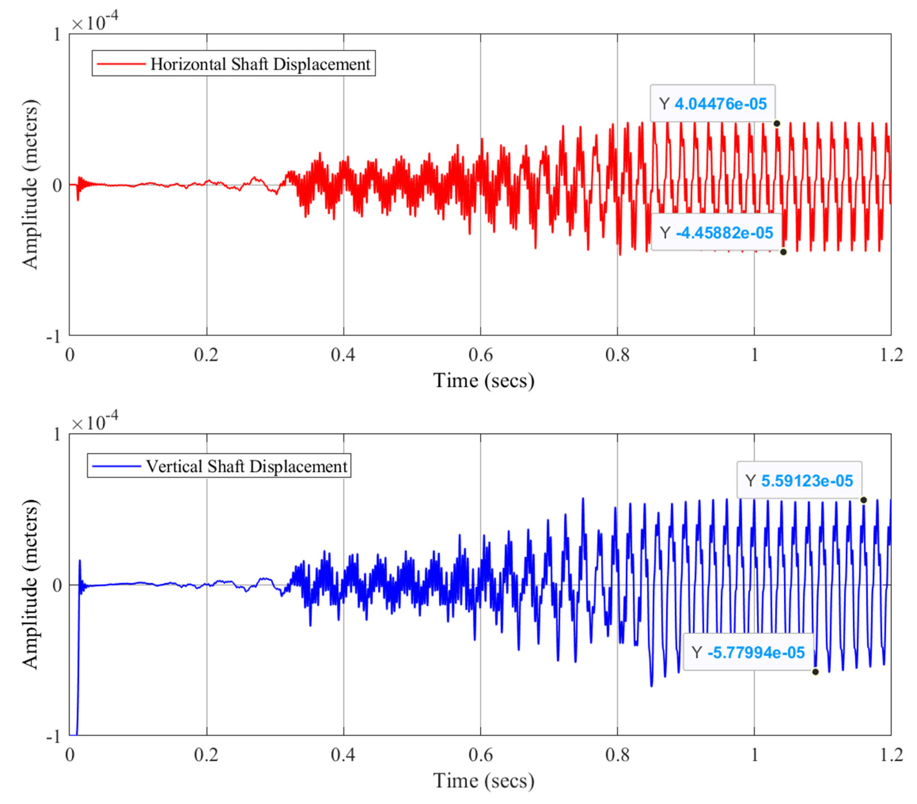
During this transition to HIL, the control performance was reduced. The shaft displacement at 3000 rpm represents the 109 and 84 µm peak-to-peaks in the vertical and horizontal directions, respectively. This corresponds to a 50% clearance between the shaft and touchdown bearing of 200 µm.

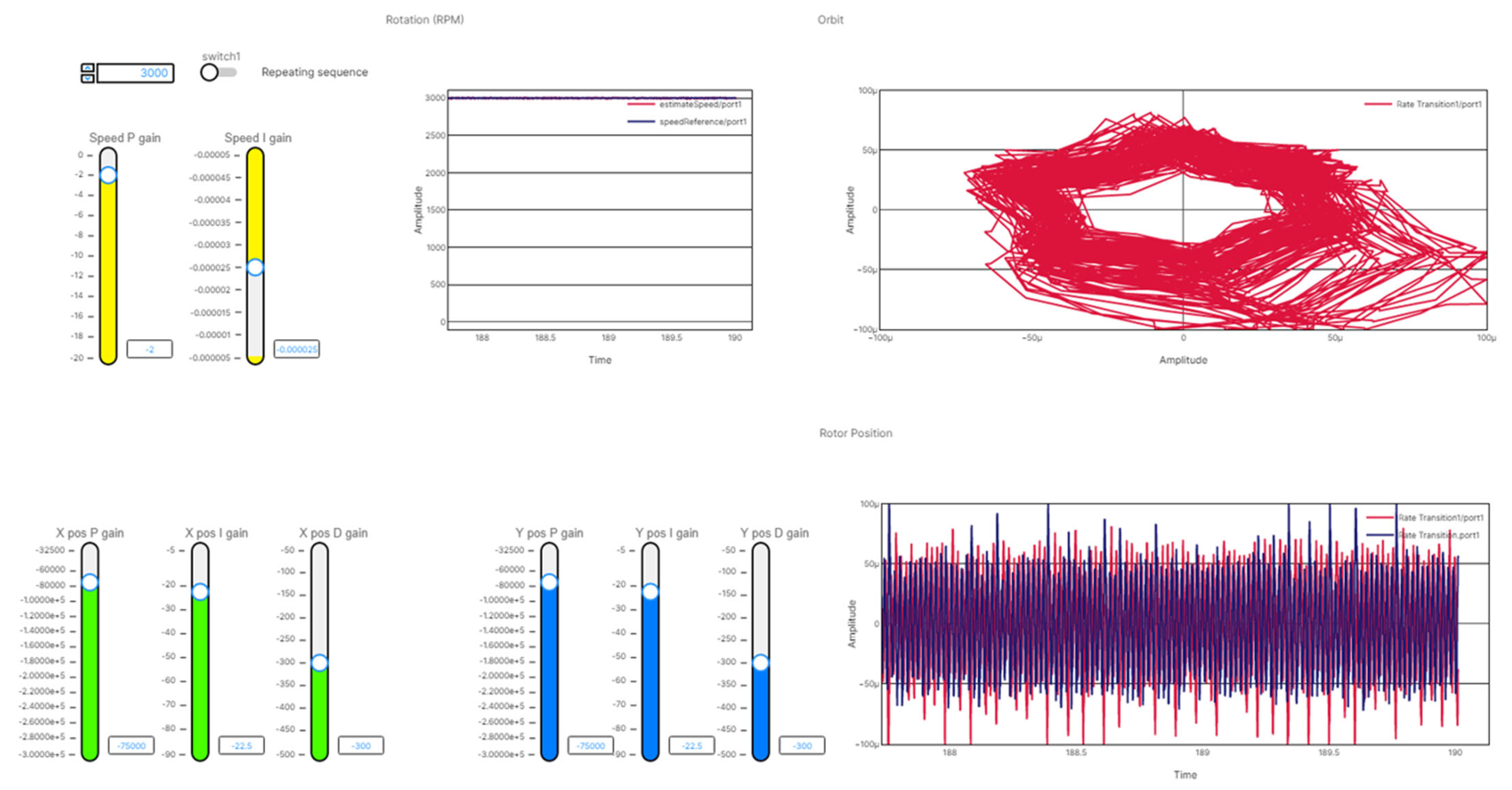
In comparison with the previous study, the results were obtained through SIMPLORER. With an ideal electrical source and continuous time, the amplitude was 18 µm peak-to-peak for both directions. After the inverters were implemented, the amplitude increased to 31 and 45 µm peak-to-peak for the horizontal and vertical directions. Figure 25 presents the dashboard of the HIL. It is possible to adjust the gain of the PI for the torque controller and PID gains for the suspension controller. Until 2750 rpm, the performance of the control is adequate, whereas at higher speeds, the rotor drags on the touchdown bearing, and this is not appropriate for operation.

6. ADRC

Active disturbance rejection control offers a modern and robust alternative to traditional control strategies by focusing on the real-time estimation and compensation of system uncertainties and external disturbances [49]. Unlike conventional model-based methods, ADRC does not rely heavily on precise mathematical models, making it particularly effective for systems with nonlinearities, time-varying parameters, or unmodeled dynamics [50].

Originally developed by Han Jingqing, ADRC was motivated by the limitations of PID controllers, which, despite their simplicity and effectiveness in linear time-invariant systems, often struggle in more complex environments [51,52]. ADRC addresses these challenges by estimating the total disturbance—a combination of external influences, model uncertainties, and nonlinear effects—and actively rejecting it through feedback control [53].

This capability distinguishes ADRC from traditional methods that typically treat disturbances as a single equivalent term or require accurate plant models [54]. A key component of ADRC is the extended state observer (ESO), which estimates both the system states and the total disturbance in real time [55]. For a more detailed explanation of the fundamentals of ADRC, refer to [56].

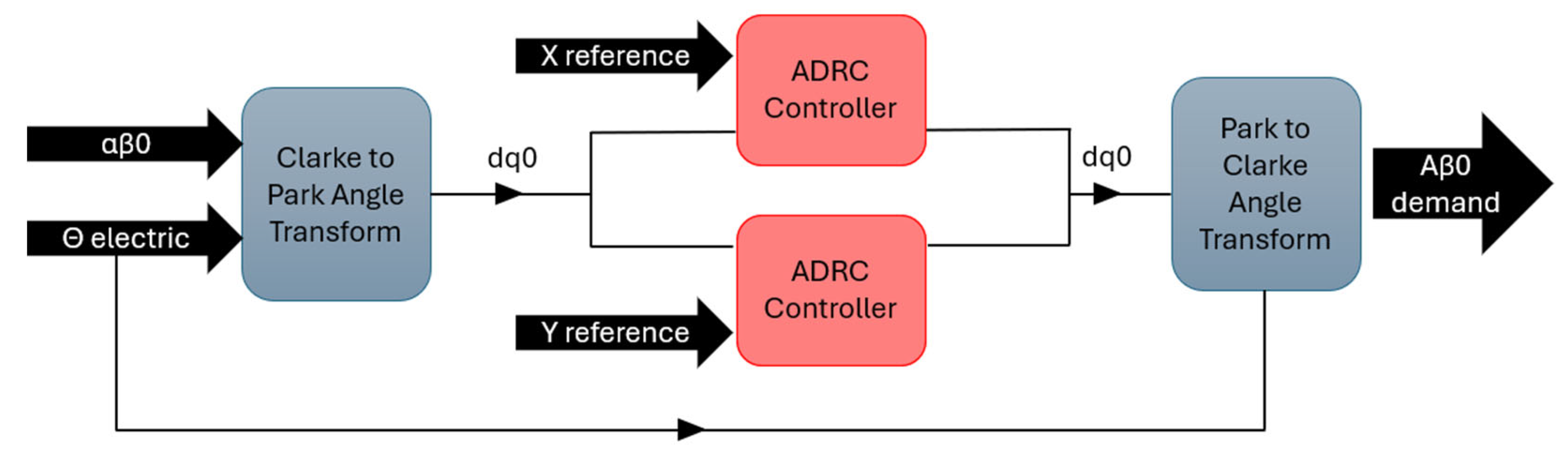
Figure 26 illustrates the integration of the ADRC controller into the internal loop of a suspension control system, replacing the conventional PI controller (as shown in the original configuration in Figure 11). This modification marks a significant advancement in control strategy for bearingless PMSMs. For a second-order plant, the key tuning parameters in the ADRC design include the plant gain ($b_0)$, the controller bandwidth (${\omega }_c$), and the observer bandwidth (${\omega }_0$).

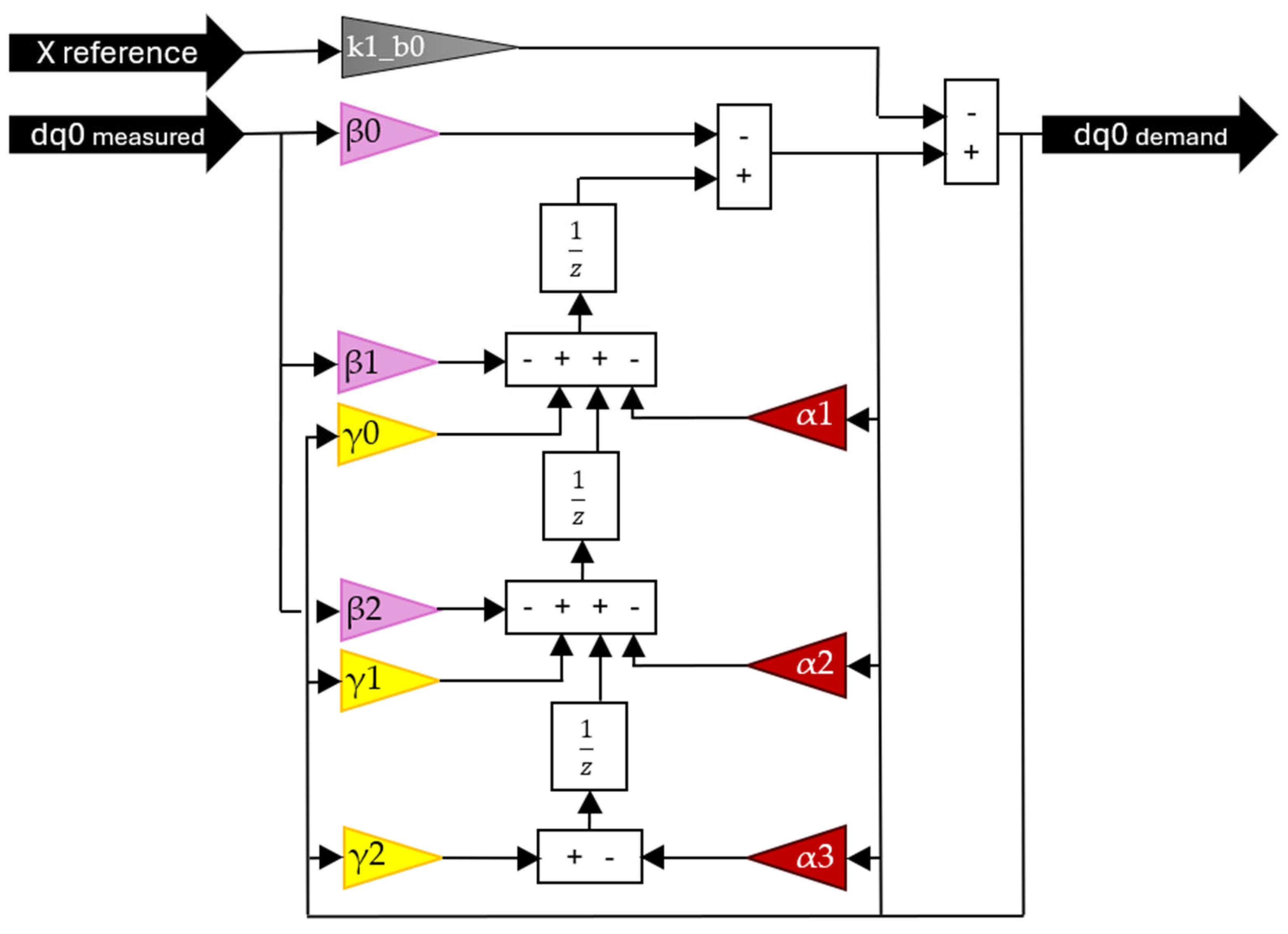
The internal structure of the ADRC controller (Figure 27) uses a discrete time dual-feedback architecture [57]. It processes the X and Y position references and measures DQ0 values through tuned coefficients (β, γ, and α) to generate the control signal. A key gain, k1_b0, scales the reference input based on the estimated plant gain and a tuning parameter, k1. For second-order systems, additional coefficients (β₂, γ₂, and α₃) are introduced to handle increased complexity. No output limitation was applied in this implementation.

The controller bandwidth ${\omega }_c$ shapes the desired closed-loop dynamics, defined by the third-order polynomial in Equation (9):

$${(s+{\omega }_c)}^3=s^3+3{\omega }_c{s}^2+3{\omega }_c^{2}s+{\omega }_c^3$$

(9)

From this expansion, the controller tuning coefficients are obtained in Equation (10) to (12) as:

$${\alpha }_1=3{\omega }_c$$

(10)

$${\alpha }_2=3{\omega }_c^2$$

(11)

$${\alpha }_3={\omega }_c^3$$

(12)

The observer bandwidth ${\omega }_0$ is a critical tuning parameter that determines how quickly the ESO estimates the system states and total disturbance. A higher observer bandwidth allows the ESO to track fast-changing disturbances and internal dynamics. For a second-order observer, the polynomial is shown in Equation (13):

$${(s+{\omega }_0)}^2=s^2+2{\omega }_{0}s+{\omega }_0^2$$

(13)

The observer tuning coefficients are derived in Equations (14) and (15) as:

$${\beta }_1=2{\omega }_0$$

(14)

$${\beta }_2={\omega }_0^2$$

(15)

The parameter tuning process was conducted using an iterative empirical approach. This involved systematically adjusting the controller gains based on the observed responses of the system to achieve a satisfactory balance between stability, responsiveness, and disturbance rejection. This trial-based methodology effectively identified suitable parameter values through successive refinements. A plant gain of 40 signifies the inherent responsiveness of the system to control inputs, with higher values indicating greater sensitivity. Conversely, a controller bandwidth of 140 rad/s dictates the aggressiveness and stability of the control action; higher values often lead to faster response times but can also induce oscillations or instability [58]. The observer bandwidth, such as with a value of 15,000 rad/s, governs the speed and accuracy with which the observer estimates the system states and disturbances.

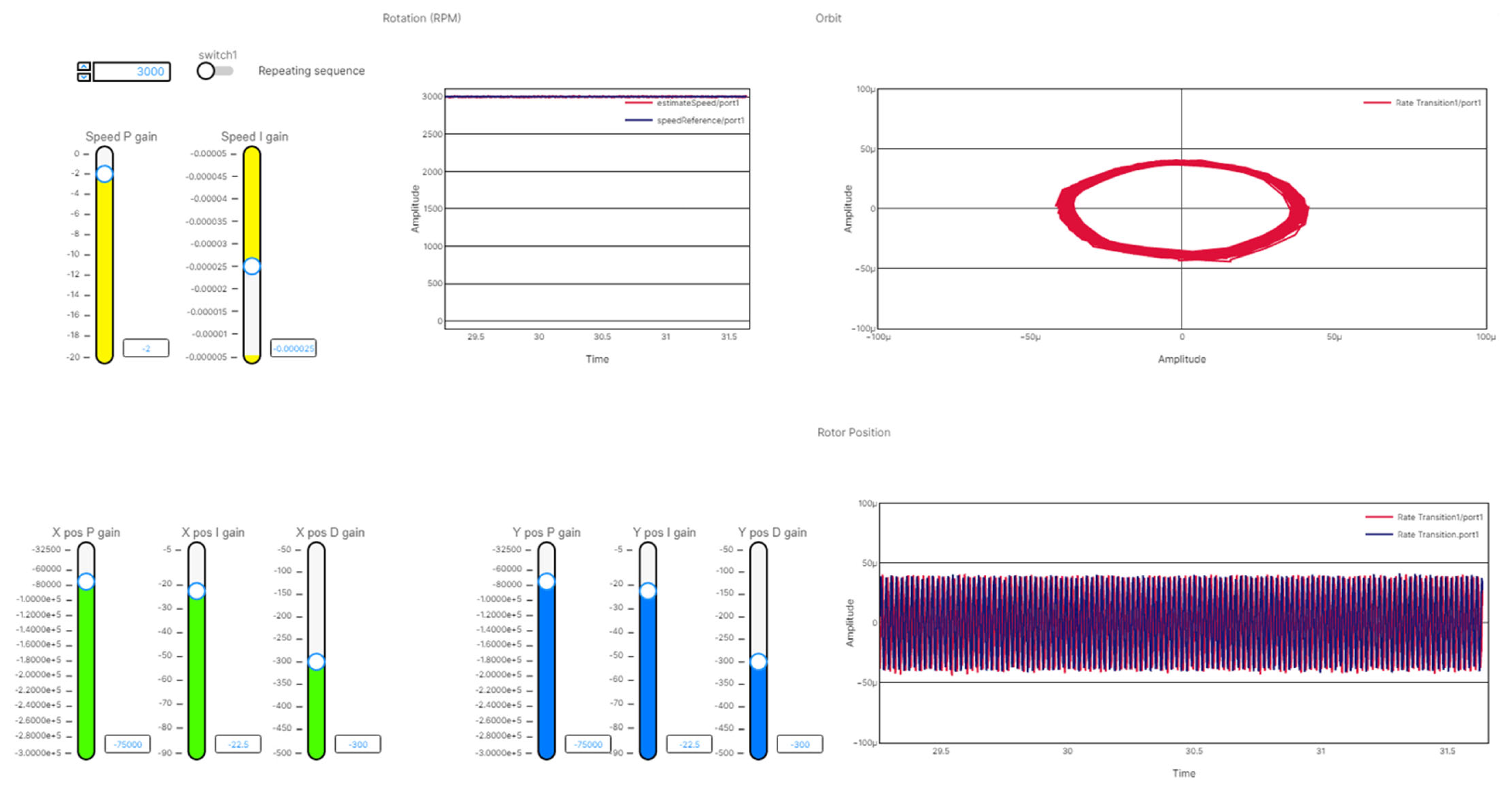
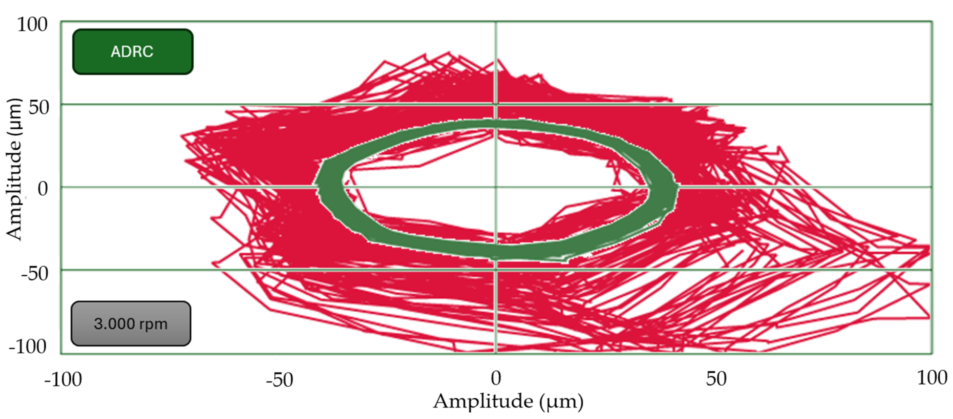
The increase in performance is notable in Figure 28 when compared to Figure 26. Figure 29 compares the orbit between two controllers. Table 2 compares the implementation in the last three columns. The implementation of ADRC reduces the amplitude by 54% and 50% in the horizontal and vertical directions, respectively.

7. Conclusions

This study presents a significant advancement in the modeling and control of BPMSMs by integrating ROM, HIL simulation, and advanced control strategies. The proposed ROM, developed using the PIM, offers a computationally efficient yet accurate representation of the coupled electromechanical dynamics of BPMSMs with combined windings, marking the first such implementation in the literature.

By bridging the gap between theoretical modeling and practical validation, this work demonstrates how HIL simulation can be effectively used to evaluate and refine control strategies without the need for costly and time-consuming physical prototypes. The use of ROMs significantly reduces computational demands while maintaining fidelity, enabling the real-time simulation and control of complex dynamic behavior.

The control strategy employed—FOC for torque and suspension, augmented by ADRC for the suspension subsystem—proves to be highly effective. As illustrated in Figure 29, the ADRC-controlled system exhibits a substantially lower orbit amplitude at 3000 rpm compared to a conventional controller, highlighting its superior disturbance rejection and dynamic performance.

Given the high cost and complexity of manufacturing bearingless motors, particularly for non-commercial, research-focused applications, this work provides a valuable alternative through virtual prototyping. The development of a high-fidelity HIL model using PIM not only reduces development time and cost but also opens new avenues for research in advanced control and system integration.

Furthermore, the results obtained with ADRC are promising and demonstrate the potential of this control strategy in managing the unique challenges posed by BPMSMs. This paper offers a structured, step-by-step methodology for evaluating such systems, contributing meaningfully to the field of motor modeling and control.

Finally, Table 2 summarizes the comprehensive study from [1] to the current condition. The initial SIMPLORER model employed an ideal current source in continuous time. Subsequent integration of the inverter and discrete-time implementation introduced signal degradation and harmonic content. Additional performance losses were observed when transitioning to the SIMULINK environment, influenced by factors such as modeling techniques, time step, and sampling frequency. The final columns of the table highlight the performance improvements achieved through the implementation of ADRC.