A Novel Control Method for Current Waveform Reshaping and Transient Stability Enhancement of Grid-Forming Converters Considering Non-Ideal Grid Conditions

Abstract

The proliferation of next-generation renewable energy systems has driven widespread adoption of electronic devices and nonlinear loads, causing grid distortion that degrades waveform quality in grid-forming (GFM) converters. Additionally, unbalanced grid faults exacerbate overcurrent risks and transient stability challenges when employing conventional virtual impedance strategies. While existing studies have separately examined these challenges, few have comprehensively addressed non-ideal grid conditions. To bridge this gap, a novel control strategy is proposed that reshapes the output current waveforms and enhances transient stability in GFM converters under such conditions. First, a sliding mode controller with an improved composite reaching law to achieve rapid reference tracking while eliminating chattering is designed. Second, a multi-quasi-resonance controller incorporating phase compensation is introduced to suppress harmonic distortion in the converter output current. Third, an individual-phase fuzzy adaptive virtual impedance strategy dynamically reshapes the current amplitude during unbalanced faults and improves the system’s transient stability. Validated through PSCAD/EMTDC simulations and hardware-in-the-loop experiments, the proposed strategy demonstrates superior transient stability and fault ride-through capability compared to state-of-the-art methods, ensuring reliable GFM converter operation under severe harmonic and unbalanced grid conditions.

1. Introduction

The accelerated global energy transition towards carbon neutrality has driven exponential growth in wind and photovoltaic installations, with renewable penetration rates exceeding 100% in certain regions [1]. However, the proliferation of power electronic devices in high-penetration scenarios introduces critical grid challenges, such as reduced system inertia and insufficient damping [2], alongside non-ideal grid characteristics, including background harmonics. Moreover, unbalanced voltage sag [3,4] is another prevalent non-ideal grid condition. As a pivotal technology for weak grid stabilization, grid-forming (GFM) converters directly influence harmonic resonance suppression capabilities in power systems and fault ride-through (FRT) performance under adverse grid operating conditions. Among various GFM control strategies, virtual synchronous generator (VSG) control demonstrates significant potential. However, existing VSG control schemes primarily address balanced grid voltages or three-phase voltage sags under harmonic-free conditions, with a predominant research focus on inertia emulation, dynamic response optimization, and stability enhancement [5,6,7,8,9,10,11]. Notably, power quality challenges under unbalanced faults and scenarios involving concurrent grid harmonics remain underexplored. Strategies developed for idealized grid operations often exhibit degraded output current performance under these non-ideal conditions, thereby undermining grid reliability. Consequently, conventional GFM control strategies face two interrelated challenges: (1) the restricted harmonic attenuation of PI controllers results in total harmonic distortion (THD) levels in converter current that exceed GB/T 33593-2017 and IEEE 1547-2018 compliance thresholds [12,13]; and (2) fixed virtual impedance (VI) parameters lack adaptability to dynamic grid disturbances, such as varying voltage sag depths and overcurrent conditions, potentially damaging the power electronic devices. These constraints necessitate advanced GFM control architectures that simultaneously enable harmonic mitigation, FRT optimization, and transient stability reinforcement under non-ideal grid conditions.

For grid harmonic mitigation, the current controller design must satisfy two core requirements: (1) achieving ideal tracking with a fast dynamic response; and (2) guaranteeing low THD in output currents. Regarding requirement 1 under non-ideal grid conditions, nonlinear control techniques demonstrate superior performance in handling system uncertainties [14,15]. Among these, sliding mode control (SMC) proves cost-effective due to its robustness, stability, fast dynamics, and inherent compatibility with power converters’ switching mechanisms [16,17,18,19,20]. For instance, [17] experimentally validates SMC in grid-tied converters, reporting faster settling times and reduced parameter sensitivity compared to conventional PI-based schemes. To address the inherent chattering phenomenon in SMC, [18] proposes a finite-time sliding mode controller for GFM converters, achieving fixed-time convergence while eliminating steady-state oscillations. Building upon the foundational SMC framework in [19], the subsequent work by [20] develops enhanced reaching law (RL) methodologies, establishing RL as a systematic framework for chattering suppression in SMC designs. To meet requirement 2, resonant controllers are widely adopted for harmonic suppression [21,22,23]. Reference [21] implements quasi-resonant controllers with explicit bandwidth and gain design rules, demonstrating superior harmonic attenuation compared to PI controllers. Reference [22] introduces a proportional multi-resonant controller in the αβ-frame to enhance the resilience of the photovoltaic system against grid distortions. However, the added compensation loops increase control complexity. A critical limitation revealed in reference [23] is the unintended phase lag introduced by multi-resonant controllers at adjacent harmonic frequencies, which may destabilize systems with tight stability margins. This underscores the necessity of integrating phase compensation mechanisms into resonant control architectures.

Furthermore, VI is conventionally employed to constrain the over-current in GFM during voltage sags to maintain grid voltage source characteristics; however, this approach creates a critical trade-off between fault current limitation and transient stability [24,25]. To address this limitation, [26] establishes an analytical framework integrating adaptive droop control and VI, which quantitatively evaluates current-limiting thresholds and critical clearing time (CCT) improvements under three-phase fault conditions. In contrast, [27] proposes a coordinated control strategy for harmonic and balanced fault current mitigation, though its applicability to unbalanced faults remains unverified. Existing unbalanced fault mitigation approaches exhibit partial effectiveness, such as incomplete harmonic suppression or delayed transient response. Reference [28] deploys αβ-frame proportional-resonant (PR) controllers with VI for unbalanced fault current limitation but neglects grid background harmonics. References [29,30] develop unified current-limiting schemes for balanced/unbalanced voltage dips, achieving effective current restraint at the expense of temporary converter output voltage depression. While [31] introduces fuzzy-PI-tuned adaptive VI for precise current clamping, its post-fault voltage recovery dynamics require further refinement.

Contemporary research predominantly focuses on strategies for either harmonic suppression or FRT, lacking a unified control architecture capable of synergistically coordinating harmonic mitigation with current-limiting functionality. This article proposes a hybrid control strategy that combines an enhanced composite reaching law with time-delay-compensated quasi-resonant control and fuzzy-adaptive VI. Designed for grid- GFM converters operating under non-ideal grid conditions featuring unbalanced faults and harmonic distortion, the strategy optimizes both waveform quality and current amplitude while enhancing transient stability. By dynamically adjusting VI parameters in response to real-time voltage sag depth and overcurrent severity, and synergizing with quasi-resonant control for targeted harmonic attenuation, the approach achieves a 60% improvement in harmonic suppression and 0° phase lag compared to conventional methods. Experimental validation confirms its ability to maintain voltage-source characteristics during unbalanced voltage sag conditions, especially at 90% for single-phase sag and 70% for two-phase sags, while limiting the current to 1.3 pu. This demonstrates the superior transient stability and operational robustness in distorted grids. The main contributions of this study include the following:

(1) A chattering-suppressed SMC is developed using an improved composite RL, which theoretically guarantees finite-time convergence as proved via Lyapunov stability criteria and shows faster tracking ability compared to traditional composite RL.

(2) A phase-compensated complex quasi-resonant control strategy is developed that simultaneously corrects the inherent plant phase lag and digital control delays, reducing both open and closed loop phase lag nearly to 0°. This approach achieves enhanced resonance regulation precision through phase compensation mechanisms.

(3) An individual-phase fuzzy-integrated adaptive VI strategy is established, which dynamically optimizes VI parameters through real-time current margin estimation and voltage sag severity analysis. This strategy simultaneously compensates for zero-sequence current impact in reference generation while enhancing active power delivery during voltage sags, achieving an improvement in the transient stability margin compared to conventional VI methods.

The paper is organized as follows. Section 2 delineates the topology and control strategies of the GFM converter. Section 3 elaborates on the current control strategy utilizing the improved composite reaching law. Section 4 details the design of the enhanced complex quasi-resonant current controller with phase compensation. Section 5 examines the individual-phase fuzzy control-based dynamic VI strategy for current limiting and transient stability improvement. Section 6 validates the proposed strategies through simulation and hardware-in-the-loop (HIL) experimentation. Section 7 discusses the limitations of the proposed method and proposes future research directions. Section 8 concludes by summarizing principal findings and contributions.

2. Topology and Control Strategies of GFM

2.1. System Description

Figure 1 illustrates the typical topology of a GFM, where U_dc denotes the DC-link voltage. Given the prevalent use of large capacitors or energy storage elements in GFM DC-links, U_dc can be considered constant. L_f represents the inductance of the LC filter, while C_f denotes the filter capacitance. The point of common coupling (PCC) current is expressed as i_PCC, with u_PCC indicating the PCC voltage. The grid impedance components are defined as L_g and R_g, and u_g represents the grid voltage.

Based on Kirchhoff’s laws, the mathematical model in the αβ stationary reference frame is established:

$$\left\{\begin{array}{l}{L}_{\mathrm{g}}{\displaystyle \frac{d{i}_{\mathsf{\alpha }}}{dt}}+R_{\mathrm{g}}{i}_{\mathsf{\alpha }}=u_{\mathrm{g}\mathsf{\alpha }}-u_{\mathrm{d}\mathrm{c}}{s}_{\mathsf{\alpha }}\hfill \\ L_{\mathrm{g}}{\displaystyle \frac{d{i}_{\mathsf{\beta }}}{dt}}+R_{\mathrm{g}}{i}_{\mathsf{\beta }}=u_{\mathrm{g}\mathsf{\beta }}-u_{\mathrm{d}\mathrm{c}}{s}_{\mathsf{\beta }}\hfill \\ C_{\mathrm{f}}{\displaystyle \frac{d{u}_{\mathrm{dc}}}{dt}}=i_a{s}_{\mathsf{\alpha }}+i_b{s}_{\mathsf{\beta }}\hfill \end{array}\right.$$

(1)

where s_α and s_β denote the switching functions of the α-axis and β-axis, respectively.

2.2. Control Strategies of GFM

The control architecture of typical VSG-type GFM converters, incorporating current limiting and saturation considerations, consist of four primary components: the active power outer-loop, the reactive power outer-loop, the VI loop, and the current inner-loop [28]. The active power control loop is designed by emulating the swing equation and primary frequency regulation, which can be expressed as follows:

$$J{\displaystyle \frac{d\omega }{dt}}={\displaystyle \frac{1}{{\omega }_{\mathrm{ref}}}}\left[P_{\mathrm{ref}}-P_{\mathrm{e}}+k_{\mathrm{f}}\left(\omega -{\omega }_{\mathrm{ref}}\right)\right]-D_p\left(\omega -{\omega }_{\mathrm{ref}}\right)$$

(2)

where J denotes the moment of inertia, ω represents the angular frequency of the virtual internal electromotive force, ω_ref indicates the reference of angular frequency and was set to 100π, P_ref corresponds to the active power reference value, P_e signifies the measured active power, D_p designates the damping coefficient, and k_f embodies the primary frequency regulation coefficient.

The reactive power control loop is designed to emulate the DC excitation and primary voltage regulation of synchronous generators, with its mathematical representation given as follows:

$$E_s=E_0+\left[Q_{\mathrm{ref}}-Q_e+k_{\mathrm{v}}\left(U_{\mathrm{ref}}-U_{\mathrm{PCC}}\right)\right]\left(k_{\mathrm{pq}}+{\displaystyle \frac{k_{\mathrm{iq}}}{s}}\right)$$

(3)

where E_s signifies the virtual internal electromotive force magnitude, E₀ denotes its reference value, Q_ref represents the reactive power reference, and Q_e indicates the measured reactive power value. k_pq and k_iq correspond to the proportional and integral coefficients of the reactive-voltage control loop, respectively.

The magnitude and phase angle of the virtual internal electromotive force can be derived from Equations (2) and (3). Based on Ohm’s law, the reference current i_ref for the current loop is obtained as follows:

$${\mathit{i}}_{\mathrm{ref}}={\displaystyle \frac{{\mathit{e}}_s-{\mathit{u}}_{\mathrm{PCC}}}{R_{\mathrm{v}}+s{L}_{\mathrm{v}}}}$$

(4)

where i_ref represents vector of current reference; e_s represents vector of virtual internal electromotive force; u_PCC represents vector of PCC voltage; and R_v and L_v denote the virtual resistance and inductance, respectively, with values adopted from [7]:

$$\left\{\begin{array}{l}{R}_{\mathrm{v}}=\max \left\{R_{\mathrm{vn}},{\displaystyle \frac{Z_{\mathrm{v}\mathrm{f}}}{\sqrt{1+{\sigma }^2}}}\right\}\\ L_{\mathrm{v}}=\max \left\{L_{\mathrm{vn}},{\displaystyle \frac{\sigma R_{\mathrm{vf}}}{{\omega }_{\mathrm{ref}}}}\right\}\end{array}\right.$$

(5)

where R_vn and L_vn denote the steady-state virtual resistance and inductance, respectively, Z_v represents the calculated transient VI value, and σ indicates the X/R ratio.

The current inner-loop regulation mechanism (e.g., PI/PR controllers) achieves accurate reference tracking upon receiving current command signals, thereby fulfilling current control objectives. Systematic investigations reveal that unbalanced operating conditions induce second-order harmonic oscillations in dq reference frames due to negative-sequence components. Conventional low-pass filtering techniques, while capable of alleviating this phenomenon, incur detrimental phase delays that compromise transient performance. The structural advantages of αβ-frame-based control architectures in preserving sinusoidal signal integrity under unbalanced grid conditions, as theoretically demonstrated in [24], have motivated the exclusive implementation of this approach in the current research. This methodological selection ensures consistent dynamic performance across various unbalanced grid scenarios while maintaining harmonic rejection capabilities.

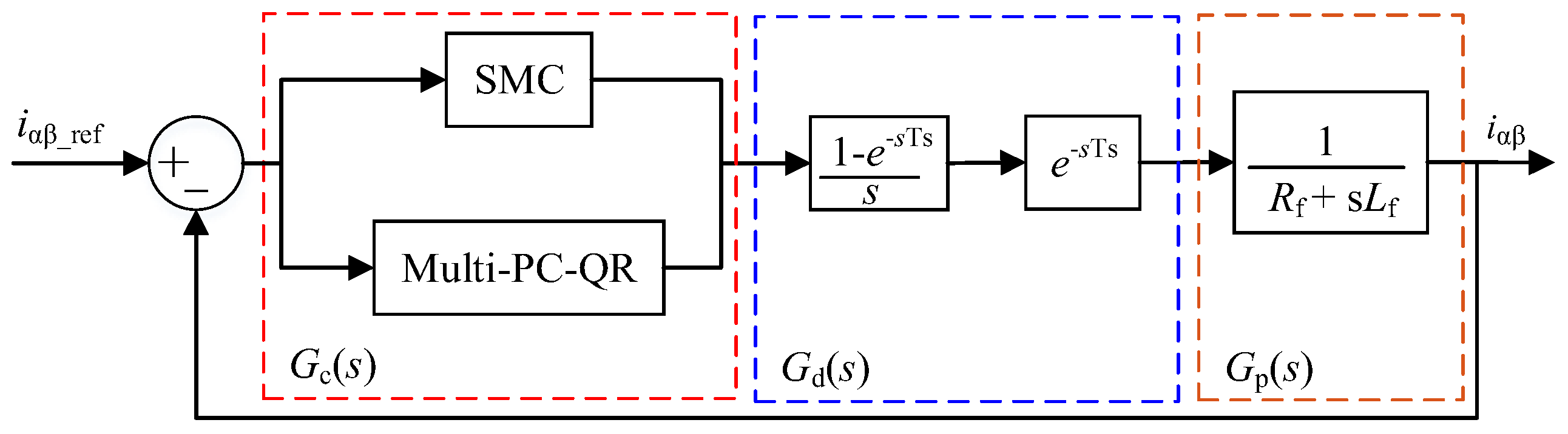
3. Improved Composite Reaching Law-Based Current Controller

3.1. Sliding Surface Selection in SMC

The fundamental concept of SMC involves designing specific sliding surfaces within the control law to drive system states toward their desired reference values. Extensive research has been conducted on sliding mode current controllers, with dual sliding surfaces established in the αβ-frame for GFM converter applications [31]. Surface s_α governs α-axis current regulation, while s_β controls β-axis current dynamics, where i_αref and i_βref denote the reference currents for their respective axes to be tracked by the control system.

$$\left\{\begin{array}{c}{s}_{\mathsf{\alpha }}\left(k\right)=i_{\mathsf{\alpha }}\left(k\right)-i_{\mathsf{\alpha }\mathrm{ref}}\left(k\right)\\ s_{\mathsf{\beta }}\left(k\right)=i_{\mathsf{\beta }}\left(k\right)-i_{\mathsf{\beta }\mathrm{ref}}\left(k\right)\end{array}\right.$$

(6)

The performance of SMC is evaluated through system tracking behavior and disturbance rejection capability. To enforce sliding motion along the manifold, the sliding vector is defined as σ = 0, with the equivalent control law $\dot{\sigma }=0$ formulated as follows:

$$\sigma =\left[\begin{array}{c}{s}_{\mathsf{\alpha }}\left(k\right)\\ s_{\mathsf{\beta }}\left(k\right)\end{array}\right]=0$$

(7)

$$\dot{\sigma }=\left[\begin{array}{c}{\dot{s}}_{\mathsf{\alpha }}\left(k\right)={\dot{i}}_{\mathsf{\alpha }}\left(k\right)-{\dot{i}}_{\mathsf{\alpha }\mathrm{ref}}\left(k\right)\\ {\dot{s}}_{\mathsf{\beta }}\left(k\right)={\dot{i}}_{\mathsf{\beta }}\left(k\right)-{\dot{i}}_{\mathsf{\beta }\mathrm{ref}}\left(k\right)\end{array}\right]=0$$

(8)

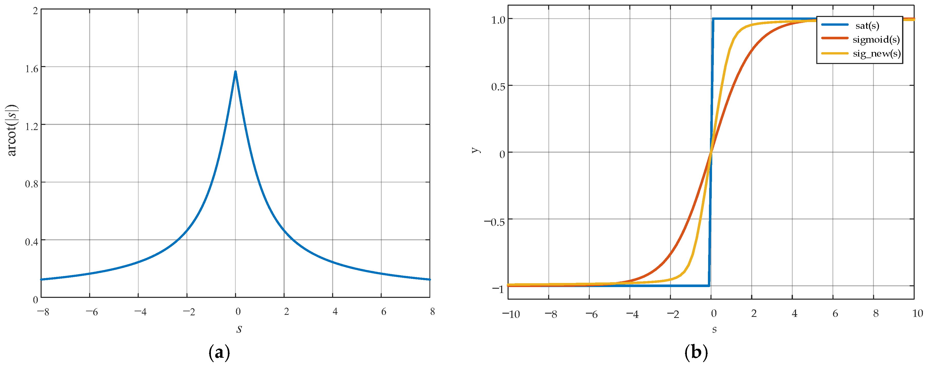
3.2. Design of an Improved Composite Reaching Law

As a prevalent method in SMC, reaching law algorithms provide an intuitive characterization of sliding-mode dynamics. Particularly during the approaching and chattering phases, the sliding variable s(k) trajectory enables precise system behavior visualization and chattering mitigation. For practical discrete-time implementations, three reaching law categories exist [32]: exponential reaching law, variable-speed reaching law, and composite reaching law combining the above two. The exponential law features fixed-width chattering bands with constant amplitude, inducing significant steady-state oscillations. The variable-speed law exhibits fan-shaped switching boundaries where chattering amplitude inversely correlates with sliding surface proximity, though initial switching transients remain severe [33].

While composite laws combine their merits, conventional implementations suffer from ambiguous switching thresholds and control discontinuity during mode transitions. This necessitates the development of novel composite reaching laws with continuous switching functions, targeting three design objectives:

(1) Enable rapid convergence toward sliding surfaces when the system operates far from them while decelerating approach speed near the surfaces to prevent overshoot.

(2) Achieve a smooth transition between exponential reaching law and variable-speed reaching law.

(3) Replace discontinuous switching functions with novel continuous counterparts.

Addressing the chattering problem induced by discontinuous control laws and fulfilling these three design objectives, an enhanced reaching law is formulated as follows:

$$\dot{s}\left(k\right)=-\left[\underset{designobjective1}{\underbrace{\left({\displaystyle \frac{1}{\frac{a\ln \left(1+e^{\left|s\left(k\right)\right|}\right)}{e^{\left|s\left(k\right)\right|}+\frac{b}{1+e^{\left|s\left(k\right)\right|}}}}}+c{e}^{\left|s\left(k\right)\right|}\ln \left(1+\left|s\left(k\right)\right|\right)\right)}}+d \underset{designobjective2}{\underbrace{\mathrm{arccot}\left(\left|s\left(k\right)\right|\right)}}\cdot {‖s\left(k\right)‖}_1\right]\underset{designobjective3}{\underbrace{\left[{\displaystyle \frac{\alpha s\left(k\right)}{{\left(1+s{\left(k\right)}^4\right)}^{\frac{1}{4}}}}+{\displaystyle \frac{\beta s\left(k\right)}{1+\left|s\left(k\right)\right|}}\right]}}$$

(9)

where parameters a, b, c, d, α, and β are positive real numbers satisfying α + β = 1, ${‖s\left(k\right)‖}_1={\displaystyle \sum _{i=1}^n\left|s{\left(k\right)}_i\right|}$ denoting the state norm of the system.

The first term addresses design objective 1, with the exponential reaching law-based function formulated such that it asymptotically approaches positive infinity as the sliding variable s tends to infinity while maintaining minimal values as s approaches zero.

The second term achieves objective 2 by integrating a smooth transition function based on the arccotangent of |s|, bridging the variable-speed reaching law and exponential reaching law, as illustrated in Figure 2a.

The third term addresses design objective 3 by developing a rate-adjustable switching function sig_new(s), advancing beyond conventional functions (e.g., sat(s) and sigmoid(s) [34]), where switching rates become tunable through parameter adaptation α and β, as illustrated in Figure 2b. This design eliminates discontinuous switching inherent to sat(s) functions while enhancing transition speed compared to sigmoid(s)-based continuous switching when α > 0.7. In this paper, 0.8 is chosen as the value of α.

3.3. Reachability and Finite-Time Convergence Analysis of Reaching Law

The proposed reaching law must satisfy both reachability and finite-time convergence criteria, ensuring the system attains the sliding surface within a finite time. Consequently, the following Lyapunov function is selected as $V\left(k\right)={\displaystyle \frac{1}{2}}s{\left(k\right)}^2$, which must comply with the discrete sliding mode existence and reachability conditions [35]. Specifically, when the sampling period T is sufficiently small, the following inequality holds:

$$\left\{\begin{array}{c}\left[s\left(k+1\right)-s\left(k\right)\right]\mathrm{sgn}\left(s\left(k\right)\right)<0\\ \left[s\left(k+1\right)+s\left(k\right)\right]\mathrm{sgn}\left(s\left(k\right)\right)>0\end{array}\right.$$

(10)

Substituting (10) into the designed approach law yields (11):

$$\left\{\begin{array}{c}\left[s\left(k+1\right)-s\left(k\right)\right]sig\_new\left(s\left(k\right)\right)=TA\left|s\left(k\right)\right|+Td\mathrm{arccot}\left(\left|s\left(k\right)\right|\right)\cdot {‖x\left(k\right)‖}_1\left|s\left(k\right)\right|<0\\ \left[s\left(k+1\right)+s\left(k\right)\right]sig\_new\left(s\left(k\right)\right)=TA\left|s\left(k\right)\right|+Td\mathrm{arccot}\left(\left|s\left(k\right)\right|\right)\cdot {‖x‖}_1\left|s\left(k\right)\right|+2\left|s\left(k\right)\right|>0\end{array}\right.$$

(11)

where

$$A={\displaystyle \frac{1}{\frac{a\ln \left(1+e^{\left|s\left(k\right)\right|}\right)}{e^{\left|s\left(k\right)\right|}}+\frac{b}{1+e^{\left|s\left(k\right)\right|}}}}+c{e}^{\left|s\left(k\right)\right|}\ln \left(1+e^{\left|s\left(k\right)\right|}\right)-{\displaystyle \frac{2}{2a+b}}-c\ln 2$$

(12)

$$sig\_new\left(s\left(k\right)\right)={\displaystyle \frac{\alpha s\left(k\right)}{{\left(1+s{\left(k\right)}^4\right)}^{\frac{1}{4}}}}+{\displaystyle \frac{\beta s\left(k\right)}{1+\left|s\left(k\right)\right|}}$$

(13)

The control law satisfies both Lyapunov stability criteria and discrete sliding mode reachability with finite-time convergence guarantees. From Equation (14) it can be shown that the control law satisfies the finite-time convergence criterion.

$$s\left(k+1\right)-s\left(k\right)=T_s\cdot A\cdot sig\_new\left(s\left(k\right)\right)+d\mathrm{arccot}\left(\left|s\left(k\right)\right|\right)\cdot {‖x‖}_{1}sig\_new\left(s\left(k\right)\right)$$

(14)

For comparative analysis, the phase trajectory of four control methods near the sliding surface (s = 0) is illustrated in Figure 3. From Figure 3, it is evident that the improved composite RL exhibits the fastest tracking speed among the four RLs. This demonstrates that the proposed enhanced composite reaching law not only achieves rapid convergence to the sliding surface but also maintains minimal chattering amplitudes, outperforming traditional composite reaching law strategies in terms of dynamic performance metrics.

3.4. Derivation of Control Law

Incorporating Equation (1) with the control objectives of sliding mode design, the output modulation signal can be selected as the equivalent control parameter:

$$\left\{\begin{array}{c}{e}_{\mathsf{\alpha }}-v_{\mathsf{\alpha }}={\dot{\sigma }}_{\mathsf{\alpha }}\\ e_{\mathsf{\beta }}-v_{\mathsf{\beta }}={\dot{\sigma }}_{\mathsf{\beta }}\end{array}\right.$$

(15)

where e_α and e_β denote the α and β components of the inner voltage phasor, while v_α and v_β represent the α and β axis components of the converter output voltage, respectively.

Therefore, this yields the current control law implemented in this work:

$$\left\{\begin{array}{c}{\dot{s}}_{\mathsf{\alpha }}=-{\displaystyle \frac{1}{L_{\mathrm{g}}}}\left(R_{\mathrm{g}}{s}_{\mathsf{\alpha }}+{\dot{\sigma }}_{\mathsf{\alpha }}+R_{\mathrm{g}}{i}_{\mathsf{\alpha }\mathrm{ref}}+L_{\mathrm{g}}{\dot{i}}_{\mathsf{\alpha }\mathrm{ref}}\right)\\ s_{\mathsf{\beta }}=-{\displaystyle \frac{1}{L_{\mathrm{g}}}}\left(R_{\mathrm{g}}{s}_{\mathsf{\beta }}+{\dot{\sigma }}_{\mathsf{\beta }}+R_{\mathrm{g}}{i}_{\mathsf{\beta }\mathrm{ref}}+L_{\mathrm{g}}{\dot{i}}_{\mathsf{\beta }\mathrm{ref}}\right)\end{array}\right.$$

(16)

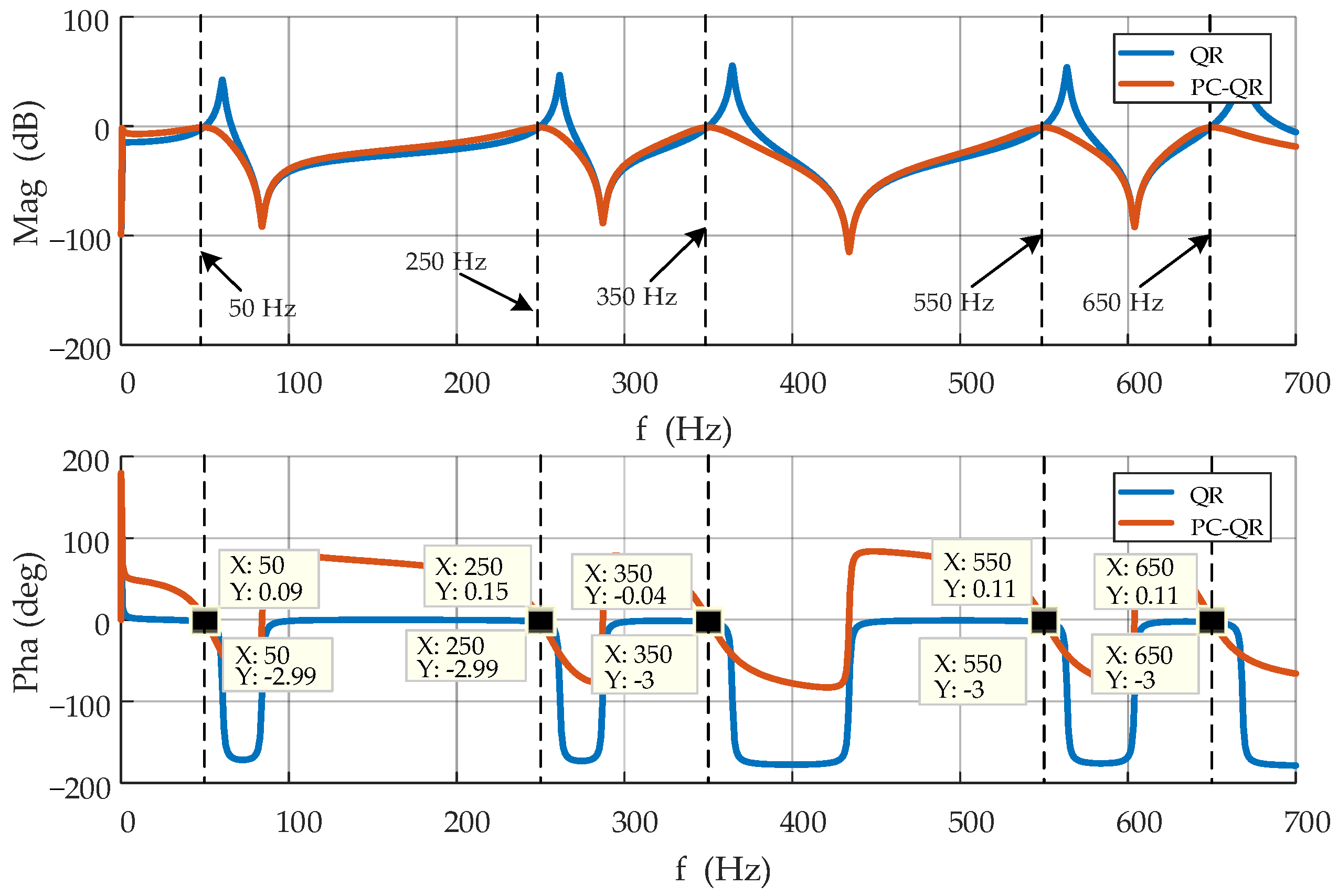
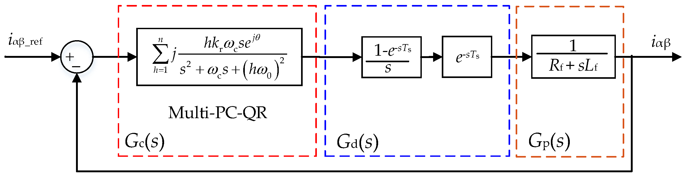
4. Improved Complex Quasi-Resonant Strategy Controller Design Considering Phase Compensation

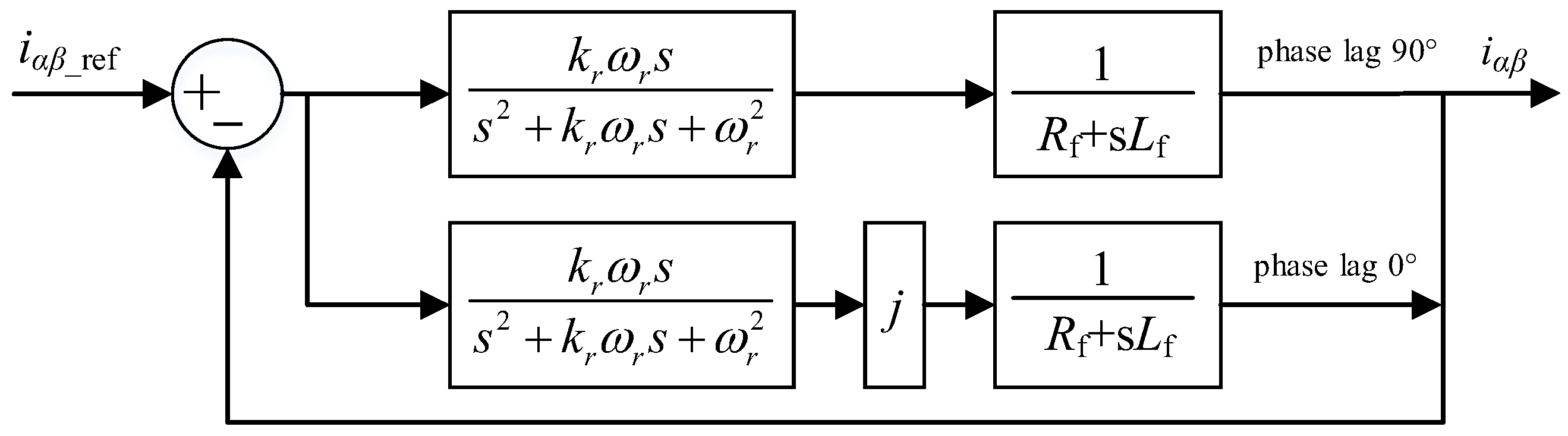
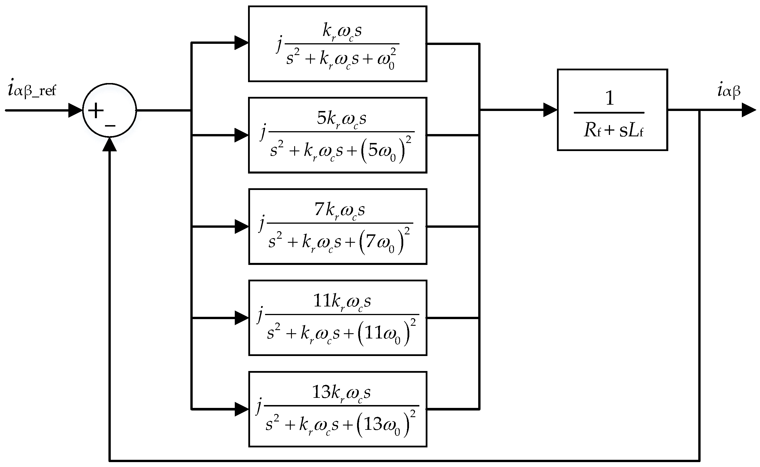
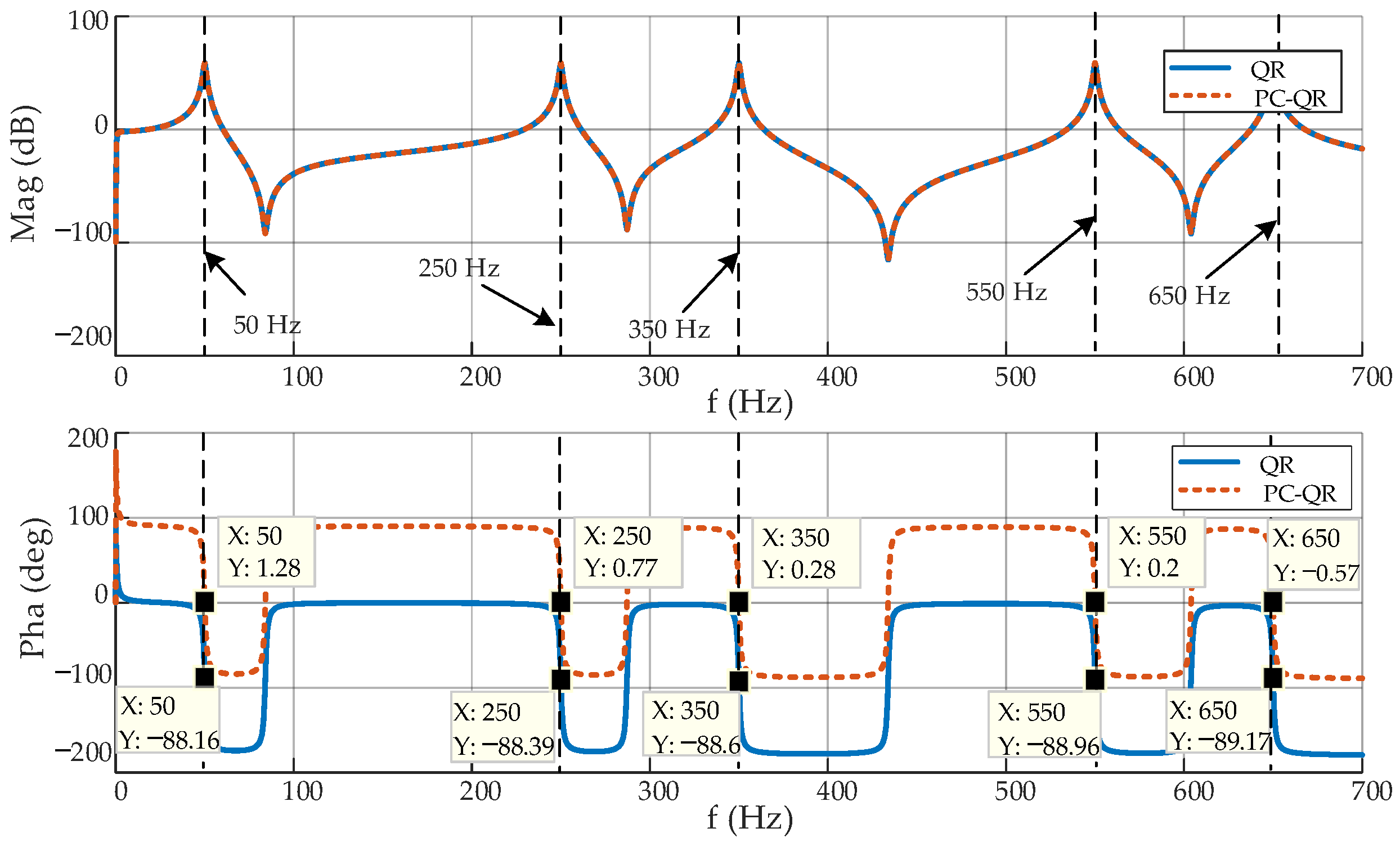
4.1. Improved Quasi-Resonant Controller Based on Phase Compensation

To control current harmonics, a PR controller is often used, which can generate infinite gain at a desired frequency, but the gain at surrounding frequencies decreases quickly, resulting in low frequency adaptability. To ensure high gain at the resonant frequency and a certain frequency bandwidth, a quasi-resonant (QR) controller is typically adopted, with its general expression as follows:

$$G_{\mathrm{QPR}}={\displaystyle \frac{k_{\mathrm{r}}{\omega }_{\mathrm{c}}s}{s^2+{\omega }_{\mathrm{c}}s+{\omega }_{\mathrm{r}}^2}}$$

(17)

where k_r is the resonance coefficient, ω_c is the resonant bandwidth, and ω_r is the resonant frequency. In this paper, k_r is chosen as 15, and ω_c is chosen as 10 rad/s.

It can be seen from Equation (17) that the phase of the original signal input remains essentially unchanged after passing through the QR controller. Considering the topology shown in Figure 1, the control plant of the current loop is:

$$G_{\mathrm{plant}}\left(s\right)={\displaystyle \frac{1}{R_{\mathrm{f}}+s{L}_{\mathrm{f}}}}$$

(18)

The inherent phase lag introduced by the plant dynamics in the current loop can be approximated as 90° since R_f is far smaller than ωL_f. To ensure high control accuracy, the open-loop transfer function must exhibit both substantial gain magnitude and a zero-phase response at the resonant frequency ω_r. Therefore, phase compensation is implemented by introducing the imaginary unit j, achieving zero-phase shift in the open-loop system for enhanced control precision. The implementation procedure is illustrated in Figure 4.

Figure 5 illustrates the control block diagram of the improved QR controller, and modeling harmonic components include the 5th, 7th, 11th, and 13th alongside the fundamental frequency under theoretical delay-free conditions. The derived open-loop transfer functions of conventional QR and PC-QR controllers are expressed as:

$$\left\{\begin{array}{c}{G}_{\mathrm{QR}\mathrm{open}}\left(s\right)={\displaystyle \sum _{h=1}^n\frac{h{k}_{\mathrm{r}}{\omega }_{\mathrm{c}}s}{s^2+{\omega }_{\mathrm{c}}s+{\left(h{\omega }_0\right)}^2}}{\displaystyle \frac{1}{R_{\mathrm{f}}+s{L}_{\mathrm{f}}}}\\ G_{\mathrm{PC}-\mathrm{QR}\mathrm{open}}\left(s\right)={\displaystyle \sum _{h=1}^{n}j\frac{h{k}_{\mathrm{r}}{\omega }_{\mathrm{c}}s}{s^2+{\omega }_{\mathrm{c}}s+{\left(h{\omega }_0\right)}^2}}{\displaystyle \frac{1}{R_{\mathrm{f}}+s{L}_{\mathrm{f}}}}\end{array}\right.$$

(19)

where h denotes the harmonic order, with its values selected as 1, 5, 7, 11, and 13.

Figure 6 compares the bode diagram of open-loop transfer functions between conventional QR and proposed phase-compensated quasi-resonant (PC-QR) controllers under parameter settings specified in Equation (19). While both exhibit identical magnitude-frequency characteristics, their phase-frequency responses demonstrate distinct behaviors. Figure 6 reveals that at the fundamental frequency, the conventional QR controller introduces approximately 90° phase lag in current open-loop output, whereas the proposed PC-QR maintains near-zero phase deviation. This phase compensation pattern persists at studied harmonic frequencies, including 5th, 7th, 11th, and 13th orders. A comparative analysis of closed-loop transfer functions derived from Figure 7 demonstrates that conventional QR generates resonant peaks near harmonic frequencies, while PC-QR effectively eliminates such undesirable amplification phenomena.

Comparative analysis of the aforementioned figures reveals two distinct advantages of the PC-QR. Firstly, the implemented phase compensation enhances the phase margin of the system, effectively mitigating phase margin insufficiency to enhance overall stability. Secondly, the phase compensation mechanism elevates control accuracy, resulting in improved control performance efficacy.

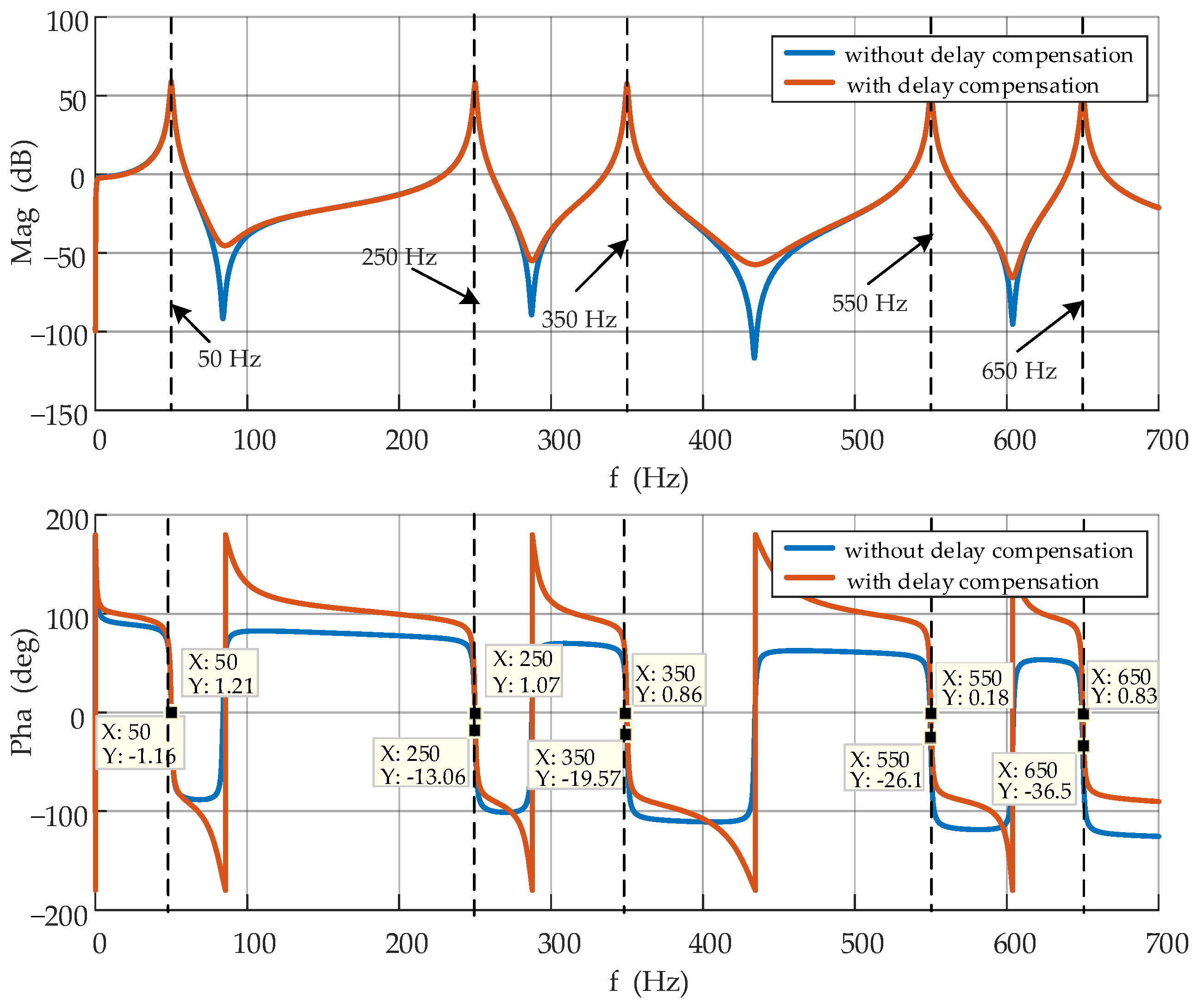
4.2. Phase Compensation Strategy

Figure 6 illustrates that phase deviation at resonance frequencies from the 0° baseline progressively increase with frequency elevation, primarily attributed to cumulative system control latency comprising sampling processes, computational delays, and zero-order hold (ZOH) effects.

Considering the time delay of the control system, the open-loop transfer function of the system is given by:

$$G_{\mathrm{close}}\left(s\right)={\displaystyle \sum _{h=1}^n\mathrm{j}\frac{h{k}_{\mathrm{r}}{\omega }_{\mathrm{c}}s}{s^2+{\omega }_{\mathrm{c}}s+{\left(h{\omega }_0\right)}^2}}{\displaystyle \frac{1-e^{-s{T}_{\mathrm{s}}}}{s}}{e}^{-s{T}_{\mathrm{s}}}{\displaystyle \frac{1}{R_{\mathrm{f}}+s{L}_{\mathrm{f}}}}$$

(20)

For the proposed enhanced QR controller with integrated phase lag compensation, the compensation design now addresses phase deviations induced by digital control delays.

$$j{\displaystyle \frac{h{k}_r{\omega }_{\mathrm{c}}s}{s^2+{\omega }_{\mathrm{c}}s+{\left(h{\omega }_0\right)}^2}}{e}^{j\theta }={\displaystyle \frac{h{k}_r{\omega }_{\mathrm{c}}s\left(-\sin \theta +j\cos \theta \right)}{s^2+{\omega }_{\mathrm{c}}s+{\left(h{\omega }_0\right)}^2}}$$

(21)

where θ equals to 1.5hω₀T_s.

The αβ-frame implementation decouples the complex variable j in controller design through real-domain transformation [36], yielding independent control laws for each axis:

$$\left\{\begin{array}{l}{u}_{\mathsf{\alpha }}^{*}=-{\displaystyle \frac{h{k}_r{\omega }_{\mathrm{c}}\sin \theta \cdot s}{s^2+{\omega }_{\mathrm{c}}s+{\left(h{\omega }_0\right)}^2}}{e}_{\mathsf{\alpha }}-{\displaystyle \frac{h{k}_r{\omega }_{\mathrm{c}}\cos \theta \cdot s}{s^2+{\omega }_{\mathrm{c}}s+{\left(h{\omega }_0\right)}^2}}{e}_{\mathsf{\beta }}\\ u_{\mathsf{\beta }}^{*}={\displaystyle \frac{h{k}_r{\omega }_{\mathrm{c}}\cos \theta \cdot s}{s^2+{\omega }_{\mathrm{c}}s+{\left(h{\omega }_0\right)}^2}}{e}_{\mathsf{\alpha }}-{\displaystyle \frac{h{k}_r{\omega }_{\mathrm{c}}\sin \theta \cdot s}{s^2+{\omega }_{\mathrm{c}}s+{\left(h{\omega }_0\right)}^2}}{e}_{\mathsf{\beta }}\end{array}\right.$$

(22)

Therefore, the control block in Figure 8 can be modified into Figure 9. Comparative open-loop bode analysis is performed to evaluate system dynamics with and without delay compensation under time-delay conditions.

To compare the effects with and without time-delay compensation (TC), the analysis is performed by examining the open-loop transfer function at a single frequency. The derived phase-frequency response expressions before and after implementing time-delay compensation are expressed as:

$$\begin{array}{ll}{\mathrm{Pha}}_{\mathrm{without}\mathrm{TC}}\left(\omega \right)& ={\mathrm{Pha}}_{\mathrm{PC}-\mathrm{QR}}+{\mathrm{Pha}}_{{\mathrm{G}}_{\mathrm{d}}(s)}+{\mathrm{Pha}}_{{\mathrm{G}}_{\mathrm{p}}(s)}\approx \mathrm{Pha}\left(j{\displaystyle \frac{h{k}_r{\omega }_{c}j\omega }{{\left(j\omega \right)}^2+{\omega }_{c}s+{\left(h{\omega }_0\right)}^2}}{e}^{j\theta }\right)+\mathrm{Pha}\left(e^{-j1.5\omega T_s}\right)+\mathrm{Pha}\left(R_{\mathrm{f}}+j\omega L_{\mathrm{f}}\right)\\ & ={90}^{\circ }-\mathrm{atan}\left({\displaystyle \frac{{\omega }_{\mathrm{c}}\omega }{{\left(h{\omega }_0\right)}^2-{\omega }^2}}\right)-1.5h\omega T_{\mathrm{s}}\end{array}$$

(23)

$$\begin{array}{ll}{\mathrm{Pha}}_{\mathrm{with}\mathrm{TC}}\left(\omega \right)& ={\mathrm{Pha}}_{\mathrm{PC}-\mathrm{QR}}+{\mathrm{Pha}}_{{\mathrm{G}}_{\mathrm{d}}(s)}+{\mathrm{Pha}}_{{\mathrm{G}}_{\mathrm{p}}(s)}\approx \mathrm{Pha}\left(j{\displaystyle \frac{h{k}_r{\omega }_{c}j\omega }{{\left(j\omega \right)}^2+{\omega }_{c}s+{\left(h{\omega }_0\right)}^2}}{e}^{j\theta }\right)+\mathrm{Pha}\left(e^{-j1.5\omega T_s}\right)+\mathrm{Pha}\left(R_{\mathrm{f}}+j\omega L_{\mathrm{f}}\right)\\ & ={90}^{\circ }-\mathrm{atan}\left({\displaystyle \frac{{\omega }_{\mathrm{c}}\omega }{{\left(h{\omega }_0\right)}^2-{\omega }^2}}\right)+1.5h{\omega }_0{T}_{\mathrm{s}}-1.5h\omega T_{\mathrm{s}}\end{array}$$

(24)

Substituting ω = hω₀ into the aforementioned equations yields:

$${\mathrm{Pha}}_{\mathrm{without}\mathrm{TC}}\left(h{\omega }_0\right)\approx -1.5h{\omega }_0{T}_{\mathrm{s}}$$

(25)

$${\mathrm{Pha}}_{\mathrm{with}\mathrm{TC}}\left(h{\omega }_0\right)\approx 0^{\circ }$$

(26)

Comparative analysis of equations. Equations (25) and (26) demonstrate that the system open-loop transfer function progressively exhibits stronger phase lag at the resonant frequency ω_r with increasing ω_r prior to time-delay compensation. In contrast, implementing TC allows the open-loop transfer function to maintain a near-zero phase shift at ω_r. The results presented in Figure 10 exhibit excellent agreement with theoretical derivations, demonstrating that the PC-QR strategy achieves phase-delay-free control of the open-loop transfer function, enabling the output signal to track the reference with zero-steady-state error while exhibiting high control accuracy and superior steady-state performance.

Furthermore, discretization methods can induce high-frequency phase aberrations in practical implementations. This study employs a pre-warped bilinear transformation method [37] for precise digital modeling:

$$s={\displaystyle \frac{{\omega }_{\mathrm{a}}}{\tan \left(\frac{{{\omega }_{\mathrm{d}}}^2}{T_s}\right)}}{\displaystyle \frac{1-z^{-1}}{1+z^{-1}}}$$

(27)

where ω_a denotes the resonant frequency in the actual discrete system, while ω_d represents its continuous-domain counterpart.

By integrating the enhanced reaching law proposed in Section 3, the control block diagram of the improved sliding mode-multiple phase compensation-quasi-resonant (SM-MPC-QR) current inner-loop architecture is derived in Figure 11.

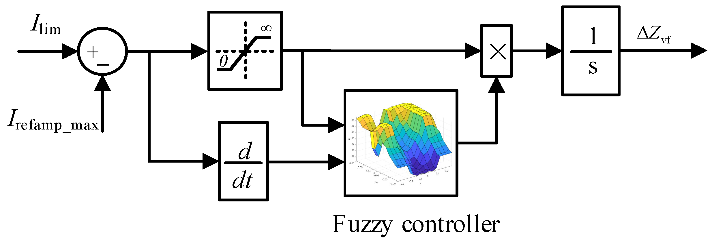
5. Individual-Phase Fuzzy Control-Based Dynamic VI Strategy for Current Limiting and Transient Stability Improvement

Adaptive VI can be divided into two parts: steady state with no overcurrent and transient state with overcurrent. Steady-state VI varies across different literature, with most values concentrated between 0.2 and 0.3 pu [38]. In this paper, steady-state VI is selected as 0.25 pu, and the X/R ratio σ is chosen as 5. To address the limitation of conventional fixed VI in adapting to faults of varying severity levels, this section introduces a transient-adaptive VI design methodology. Considering that fuzzy control exhibits high robustness, wide adaptability, and fast response without relying on an accurate model of the controlled system, this paper considers the use of the fuzzy control strategy. Furthermore, existing methods based on VI can only inhibit overcurrent, and none of them can accurately limit the current to the desired limit. To address this issue, a feedforward-based fuzzy integral correction link can be designed to calculate the transient impedance required for the transient state through approximate calculations. This approach allows the current to reach the specified limit via integral control, ensuring that the grid-forming (GFM) converter operates at the equilibrium point, inhibits overcurrent, and improves transient stability.

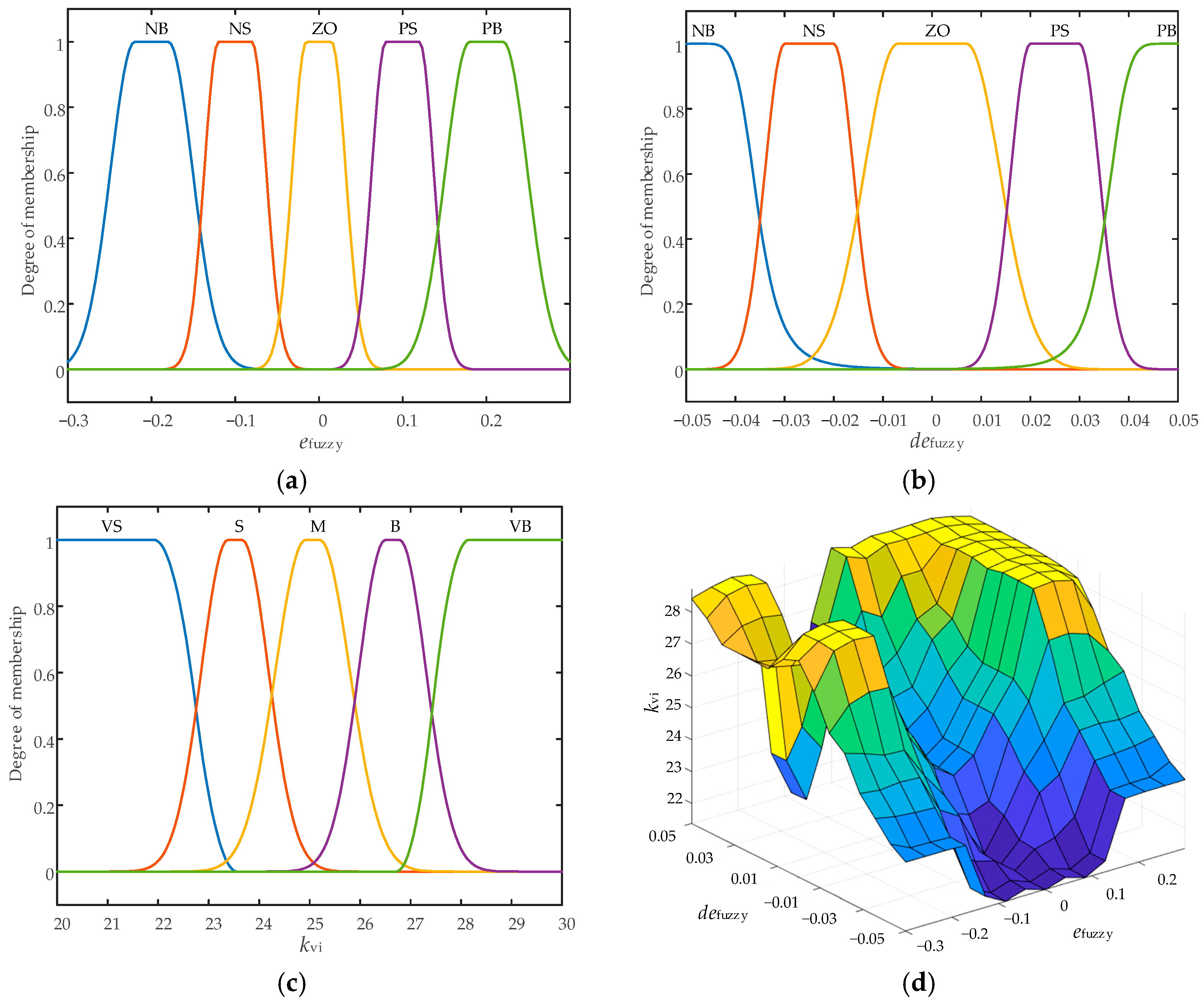
5.1. Fuzzy-Based Transient Adaptive VI Strategy for Current Limitation

Assuming that a phase current reaches the current limit value, the magnitude of the VI Z_vf0 required to limit the current to I_lim can be calculated according to the relationship between the internal potential and the voltage at the PCC as follows:

$$Z_{\mathrm{vf}0}={\displaystyle \frac{\sqrt{E^2+{U_{PCC}}^2-2E{U}_{PCC}\cos \theta }}{I_{\lim }}}$$

(28)

where E represents the amplitude of the inner voltage phasor, U represents the amplitude of voltage phasor at the PCC, and θ represents the angle between the two vectors.

Measurement inaccuracies and practical constraints render pure VI feedforward insufficient for precise current limiting threshold acquisition, necessitating compensatory adjustment modules for VI calibration. Therefore, this section develops an adaptive correction module demonstrated in Figure 12, incorporating fuzzy-integral coefficients that dynamically adjust VI parameters to constrain peak phase currents within rated thresholds.

The input–output mapping logic of this fuzzy-based correction module is designed as follows: for current limiting objectives, when the current reference amplitude is below the threshold, moderate corrective actions prevent transient overcurrent spikes; conversely, aggressive correction coefficients are activated under severe overcurrent conditions to achieve rapid mitigation. The algorithm takes the overcurrent status and its dynamic variation as inputs, denoted as e_fuzzy and de_fuzzy.

$$e_{\mathrm{fuzzy}}=I_{\lim }-I_{\mathrm{refamp}\_\max }$$

(29)

$$d{e}_{\mathrm{fuzzy}}={\displaystyle \frac{d{e}_{\mathrm{fuzzy}}}{dt}}$$

(30)

where I_lim denotes the current-limiting threshold, which is determined by the overcurrent capability of the power electronic devices and typically ranges from 1.2 to 1.5 pu. In this study, I_lim is selected as 1.3 pu. I_{refamp_max} represents the highest reference current amplitude, calculated as follows:

$$I_{\mathrm{refamp}\_\max }=\max \left\{I_{\mathrm{refa}\_\mathrm{amp}},I_{\mathrm{refb}\_\mathrm{amp}},I_{\mathrm{refc}\_\mathrm{amp}}\right\}$$

(31)

Considering the resolution and computational constraints of fuzzy control systems, the overcurrent deviation e_fuzzy and its derivative de_fuzzy are quantized into five linguistic variables: Negative Big (NB), Negative Small (NS), Zero (ZO), Positive Small (PS), and Positive Big (PB). Their discrete universes of discourse are defined as {−0.5, −0.3, 0, 0.3, 0.5} for e_fuzzy and {−0.05, −0.03, 0, 0.03, 0.05} for de_fuzzy, respectively. To enhance stabilization capability during operation near 1.3 pu, larger integral coefficients are activated when current deviations reach e_fuzzy = ±0.3 to enable rapid current regulation, where the boundary linguistic terms (NB/PB) utilize generalized bell-shaped membership functions for swift response characteristics. The intermediate terms (NS/ZO/PS) employ joint Gaussian membership functions to ensure smooth output transitions. The control output is the integral coefficient k_i with a discrete universe of {20, 23.5, 25, 26.5, 30}, mapped to linguistic variables: Very Small (VS), Small (S), Medium (M), Big (B), and Very Big (VB). The designed fuzzy control rules are summarized in

Table 1. Fuzzy control law.

		e
		NB	NS	ZO	PS	PB
de	NB	VS	VS	S	S	M
	NS	VS	VS	S	M	B
	ZO	S	S	S	B	B
	PS	S	M	S	VB	VB
	PB	M	B	VB	VB	VB

, with input–output membership functions illustrated in Figure 13a–c and the control rule surface displayed in Figure 13d.

The result of fuzzy reasoning depends on the defuzzification process. In this paper, the gravity center method is adopted for defuzzification, expressed as:

$$k_{\mathrm{vi}}={\displaystyle \frac{{\displaystyle \sum _{i=1}^{M}u{\left(e_{\mathrm{fuzzy}}\right)}_{i}u{\left(d{e}_{\mathrm{fuzzy}}\right)}_i{\left(k_{\mathrm{vi}}\right)}_i}}{{\displaystyle \sum _{i=1}^{M}u{\left(e_{\mathrm{fuzzy}}\right)}_{i}u{\left(d{e}_{\mathrm{fuzzy}}\right)}_i}}}$$

(32)

where μ(e)_i is the membership of the ith e(t), and μ(de)_i is the membership of the ith de(t).

It is worth emphasizing that the variation of the equivalent output impedance during a fault does not affect the operating principle of the converter, which still maintains its GFM behavior during such operating condition. The calculations for Z_vf, R_vf, and L_vf are performed as follows:

$$\left\{\begin{array}{l}{Z}_{\mathrm{vf}}=Z_{\mathrm{vf}0}+\Delta Z_{\mathrm{vf}}\\ R_{\mathrm{vf}}={\displaystyle \frac{Z_{\mathrm{vf}}}{\sqrt{1+{\sigma }^2}}}\\ L_{\mathrm{vf}}={\displaystyle \frac{\sigma R_{\mathrm{vf}}}{{\omega }_{\mathrm{n}}}}\end{array}\right.$$

(33)

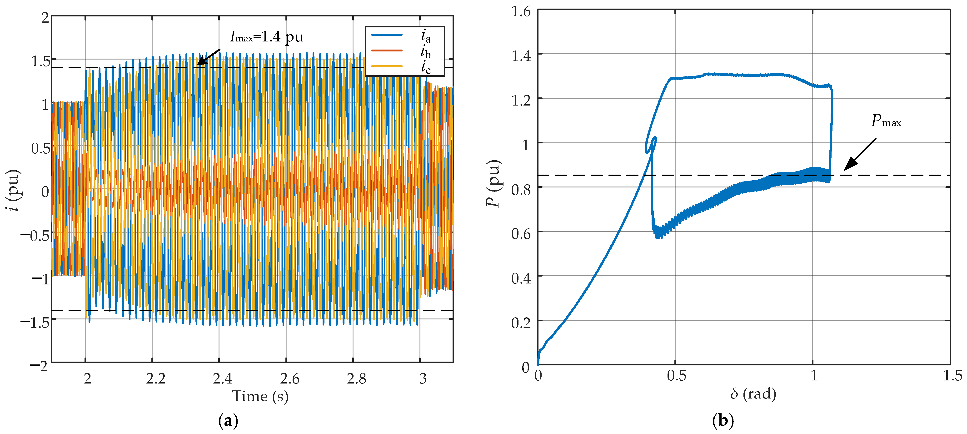
5.2. Investigation of Current Limiting and Transient Stability Under Unbalanced Voltage Sag

5.2.1. Study of Current Limiting Strategies for Unbalanced Voltage Sag

Given that single-phase voltage sags exhibit the highest occurrence probability among unbalanced grid faults, subsequent analyses adopt phase-A voltage sag as the representative case study. With identical three-phase virtual impedances, Equation (4) analytically demonstrates that the fault-phase current reference attains the maximum magnitude during phase-A voltage sag conditions. To ensure that the highest phase current remains within permissible limits, the scaling factor k is derived as follows [39]:

$$k=\left\{\begin{array}{cc}{\displaystyle \frac{I_{\max }}{I_{\mathrm{ref}\_\max }}}& ,I_{\mathrm{ref}\_\max }>I_{\max }\\ 1& ,I_{\mathrm{ref}\_\max }\le I_{\max }\end{array}\right.$$

(34)

where I_max represents the maximum current amplitude among three phases and is selected as 1.4 pu in this study.

Therefore, the new current reference values obtained after applying three-phase identical scaling are expressed as follows:

$$\left\{\begin{array}{c}{i}_{\mathrm{refnew}\_\mathrm{a}}=k\cdot I_{\mathrm{refa}}\\ i_{\mathrm{refnew}\_\mathrm{b}}=k\cdot I_{\mathrm{refb}}\\ i_{\mathrm{refnew}\_\mathrm{c}}=k\cdot I_{\mathrm{refc}}\end{array}\right.$$

(35)

For unbalanced faults, however, current usually cannot be limited to the desired threshold when using basic current control methods [40]. Additionally, the application of three-phase identical scaling factors presents two primary challenges. First, using the phase current with maximum amplitude as the reference basis results in oversizing scaling coefficients being applied to all three phases, leading to reduced active power output and compromised transient stability. Second, during unbalanced grid faults, the derived current references contain zero-sequence components. However, the three-phase three-wire converter topology inherently prevents zero-sequence current generation under normal operation. This characteristic introduces non-eliminable steady-state errors within the control loop, leading to imprecise regulation in the current control loop and diminished effectiveness of current limiting mechanisms. Figure 14 presents simulation results obtained with parameters from

Table 2. Parameters used in the simulation and experiment.

Quantity	Symbol	Value	Units
Grid Parameters
Rated voltage	Un	0.4	kV
Rated angular frequency	ω0	100π	rad/s
Gird impedance	Lg	1.133	mH
Filter inductance	Lf	0.2	pu
Filter capacitance	Cf	0.05	pu
Inverter Parameters
Rated capacity	Sn	0.0346	MW
Static Virtual inductance	Lv_n	0.3	pu
Static Virtual resistance	Rv_n	0.06	pu
DC voltage	Udc	1.1	kV
Sample frequency	fs	9	kHz
Damping coefficient	Dp	3.5 × 10−5	N.m.s/rad
Inertia constant	H	2.0	s
Speed governor coefficient	kω	20	pu
Reactive power control loop proportional coefficient	kpv	0.1	pu
Reactive power control loop integral coefficient	kiv	20
SMC parameters	a	1.25
	b	10.0
	c	0.05
	d	0.005
	α	0.8
X/R ratio	σ	5

, using phase A voltage sag down to 0.1 pu as a case study, which clearly demonstrates the aforementioned issues. As illustrated in Figure 14a, the presence of zero-sequence current introduces steady-state errors in current regulation, causing phase currents to exceed the maximum threshold I_max and violate current limitation requirements. Figure 14b reveals that the transient active power output reaches a minimum of 0.6 pu, with the acceleration area exceeding that of the maximum-power-maintenance scenario, indicating substantial potential for transient stability improvement through control optimization.

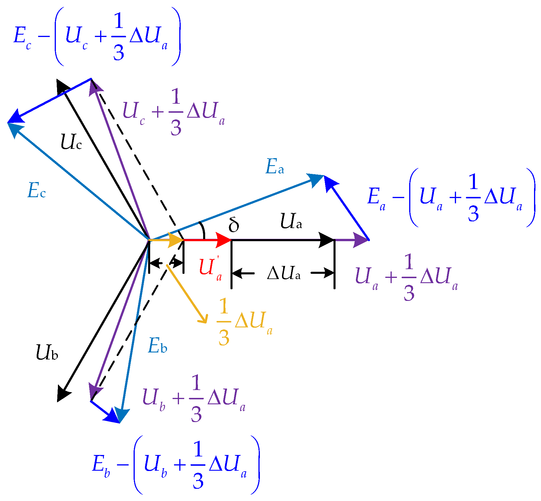
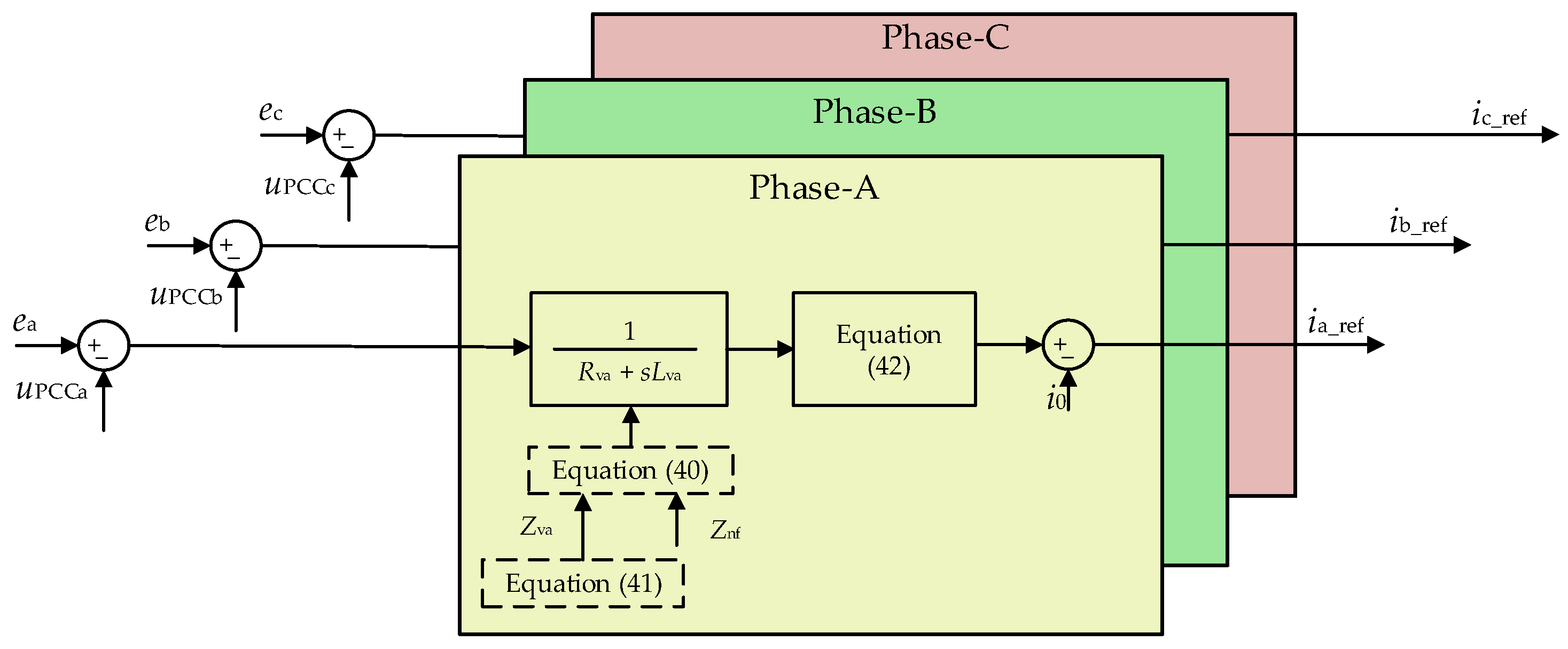
5.2.2. Individual-Phase VI Strategy for Transient Stability Enhancement via Zero-Sequence Current Separation

Effects of Zero-Sequence Current

This subsection investigates the overcurrent phenomenon induced by zero-sequence currents as identified in Section 5.2.1, with the objective of mitigating their adverse effects on current limiting performance. To rigorously characterize these interactions, this investigation employs space vector analysis to quantify zero-sequence current dynamics within the control architecture, supported by the following mathematical representation:

$$i_{ref0}={\displaystyle \frac{1}{3}}\left(i_{\mathrm{refa}}+i_{\mathrm{refb}}+i_{\mathrm{refc}}\right)$$

(36)

where i_ref0 denotes the zero-sequence component in current references, while i_refa, i_refb, i_refc represent phase-specific current references for phases a, b, and c, respectively.

Combining Equations (4) and (36) yields:

$${\mathit{I}}_{\mathrm{ref}0}={\displaystyle \frac{1}{3}}\left({\displaystyle \frac{{\mathit{E}}_{\mathrm{a}}-{\mathit{U}}_{\mathrm{a}}}{R_{\mathrm{a}}+j{\omega }_{\mathrm{N}}{L}_{\mathrm{a}}}}+{\displaystyle \frac{{\mathit{E}}_{\mathrm{b}}-{\mathit{U}}_{\mathrm{b}}}{R_{\mathrm{b}}+j{\omega }_{\mathrm{N}}{L}_{\mathrm{b}}}}+{\displaystyle \frac{E_{\mathrm{c}}-U_{\mathrm{c}}}{R_{\mathrm{c}}+j{\omega }_{\mathrm{N}}{L}_{\mathrm{c}}}}\right)$$

(37)

To investigate the impact of zero-sequence current components in current references under unbalanced fault conditions, this analysis assumes identical three-phase VI parameters: R_v and L_v. Given the prevalence of single-phase voltage sags in practical grid scenarios, subsequent analyses focus predominantly on single-phase voltage sag scenarios. Taking the voltage sag of phase A as an example, since the potential in the output of the GFM is always balanced, the Equation (37) can be simplified as follows:

$${\mathit{I}}_{ref0}=-{\displaystyle \frac{1}{3}}\left({\displaystyle \frac{{\mathit{U}}_{\mathrm{a}}+{\mathit{U}}_{\mathrm{b}}+{\mathit{U}}_{\mathrm{c}}}{R_{\mathrm{v}}+j{\omega }_{\mathrm{N}}{L}_{\mathrm{v}}}}\right)={\displaystyle \frac{1}{3}}{\displaystyle \frac{\Delta {\mathit{U}}_{\mathrm{a}}}{R_{\mathrm{v}}+j{\omega }_{\mathrm{N}}{L}_{\mathrm{v}}}}$$

(38)

where ΔU_a represents the change of phase A voltage.

Since the steady-state VI value Z_vn = 0.25 pu, the influence of the zero-sequence current on the reference current cannot be ignored and must be considered in the design range. To eliminate the influence of zero sequence current, directly subtract i_ref0 from the original three-phase current reference value generated by VI, resulting in a newly generated three-phase current reference value:

$$\left\{\begin{array}{c}{\mathit{I}}_{\mathrm{refa}\_\mathrm{new}}={\displaystyle \frac{{\mathit{E}}_a-{\mathit{U}}_a}{R_v+j{\omega }_N{L}_v}}-{\mathit{I}}_{ref0}={\displaystyle \frac{{\mathit{E}}_a-\left({\mathit{U}}_a+\frac{1}{3}\Delta {\mathit{U}}_a\right)}{R_v+j{\omega }_N{L}_v}}\\ {\mathit{I}}_{\mathrm{refb}\_\mathrm{new}}={\displaystyle \frac{{\mathit{E}}_b-{\mathit{U}}_b}{R_v+j{\omega }_N{L}_v}}-{\mathit{I}}_{ref0}={\displaystyle \frac{{\mathit{E}}_b-\left({\mathit{U}}_b+\frac{1}{3}\Delta {\mathit{U}}_a\right)}{R_v+j{\omega }_N{L}_v}}\\ {\mathit{I}}_{\mathrm{refc}\_\mathrm{new}}={\displaystyle \frac{{\mathit{E}}_{\mathrm{c}}-{\mathit{U}}_{\mathrm{c}}}{R_v+j{\omega }_N{L}_v}}-{\mathit{I}}_{ref0}={\displaystyle \frac{{\mathit{E}}_{\mathrm{c}}-\left({\mathit{U}}_{\mathrm{c}}+\frac{1}{3}\Delta {\mathit{U}}_a\right)}{R_v+j{\omega }_N{L}_v}}\end{array}\right.$$

(39)

The relative magnitudes of the current after subtracting the zero-sequence current can be obtained by analyzing the voltage vector of each phase, as depicted in Figure 15.

The resultant voltage vector can be derived from Figure 15. It is evident that in the resultant voltage vector represented by the blue lines, phase C exhibits the maximum amplitude, followed by phase A and phase B. Therefore, after removing the zero-sequence current from the current reference value, the relationship between the three-phase current sizes is as follows: i_{cref_new} > i_{aref_new} > i_{bref_new}. Similarly, the analysis of other phases during single-phase faults leads to the conclusion that when a single-phase voltage sag occurs, the phase with the highest current usually produces the leading phase closest when the voltage sag happens. This conclusion is confirmed by the simulation results in Figure 16, which are consistent with the theoretical analysis. The analysis of the effect of zero sequence current on the two-phase voltage sag is fundamentally similar, so it will not be elaborated here.

Figure 16 displays simulation waveforms under identical conditions with zero-sequence components subtracted from the reference current. The results demonstrate that the processed current—obtained by eliminating zero-sequence components from reference values—remains effectively constrained within I_max without inducing overcurrent conditions. Furthermore, the amplitude-dependent constraints derived from the aforementioned phase current analysis effectively inhibit concurrent attainment of current saturation thresholds across all three phases under fault conditions.

Transient Stability Enhancement Analysis

To address the limitations of the three-phase unified current reduction strategy described in Section 5.2—specifically, the reduced active power output after a voltage sag and enlarged system acceleration area—this section proposes an individual-phase VI method for transient stability enhancement. The proposed method implements two key modifications: transitioning from three-phase unified control to individual-phase independent control of VI loop and applying phase-specific proportional reduction coefficients for overcurrent phases. This strategy increases the short-circuit current capacity of GFM converters during faults, while also improving transient stability margins. Notably, single-phase dq transformation is implemented for rapid and accurate phase current amplitude extraction across all phases [41]. This is achieved by reformulating Equations (5), (33) and (34) into single-phase implementations that directly govern individual phase currents, which can be changed as:

$$\left\{\begin{array}{l}{R}_{\mathrm{vx}}=\max \left\{R_{\mathrm{vn}},{\displaystyle \frac{Z_{\mathrm{vfx}}}{\sqrt{1+{\sigma }^2}}}\right\}\\ L_{\mathrm{vx}}=\max \left\{L_{\mathrm{vn}},{\displaystyle \frac{\sigma R_{\mathrm{vfx}}}{{\omega }_{\mathrm{ref}}}}\right\}\end{array}\right.$$

(40)

$$Z_{\mathrm{vfx}}=Z_{\mathrm{vfx}0}+\Delta Z_{\mathrm{vfx}}$$

(41)

$$k_{\mathrm{x}}=\left\{\begin{array}{cc}{\displaystyle \frac{I_{\max }}{I_{\mathrm{refx}}}}& ,I_{\mathrm{refx}}>I_{\max }\\ 1& ,I_{\mathrm{refx}}\le I_{\max }\end{array}\right.$$

(42)

where x = a, b, c corresponds to phase A, phase B, and phase C respectively.

The implementation architecture of the proposed individual-phase VI strategy is illustrated in Figure 17.

Under the individual-phase VI strategy, the active power output P_{ind_VI} of the GFM converter is formulated as follows:

$$P_{\mathrm{ind}-\mathrm{VI}}=k_{\mathrm{a}}{u}_{\mathrm{a}}{i}_{\mathrm{aref}}+k_b{u}_{\mathrm{b}}{i}_{\mathrm{bref}}+k_{\mathrm{c}}{u}_{\mathrm{c}}{i}_{\mathrm{cref}}$$

(43)

In contrast, the conventional three-phase unified VI strategy yields the active power output P_{uni_VI}, expressed as:

$$P_{\mathrm{uni}\_\mathrm{VI}}=k\left(u_{\mathrm{a}}{i}_{\mathrm{aref}}+u_{\mathrm{b}}{i}_{\mathrm{bref}}+u_{\mathrm{c}}{i}_{\mathrm{cref}}\right)$$

(44)

Based on the current magnitude relationships established under unbalanced voltage sags in the preceding section, during overcurrent conditions, the aforementioned Equations (43) and (44) undergo modification as follows:

$$P_{\mathrm{ind}-\mathrm{VI}}=u_{\mathrm{a}}{i}_{\mathrm{aref}}+u_{\mathrm{b}}{i}_{\mathrm{bref}}+k_{\mathrm{c}}{u}_{\mathrm{c}}{i}_{\mathrm{cref}}$$

(45)

$$P_{\mathrm{uni}\_\mathrm{VI}}=k_{\mathrm{c}}\left(u_{\mathrm{a}}{i}_{\mathrm{aref}}+u_{\mathrm{b}}{i}_{\mathrm{bref}}+u_{\mathrm{c}}{i}_{\mathrm{cref}}\right)$$

(46)

Given that k_c < 1, it follows that P_{uni_VI} < P_{ind_VI}. Comparative simulation waveforms evaluating the transient stability characteristics of both control strategies are presented in Figure 18. Identical experimental conditions were maintained for both methodologies to enable a rigorous transient stability performance. As evidenced in Figure 18, the individual-phase VI strategy enhances active power output during transients while achieving a reduced deceleration area. This demonstrates superior transient stability performance compared to the conventional three-phase unified VI strategy.

6. Simulation and Experimental Verification

The control block diagram of the current waveform reshaping and transient stability enhancement strategy for GFM converters under non-ideal grid conditions is shown in Figure 19. To validate the effectiveness of the proposed control strategy, simulation and HIL experimental verification were conducted using PSCAD/EMTDC simulation software (V4.6.0) and Typhoon HIL platform, respectively. The parameters of the simulation and experiment are shown in Table 2.

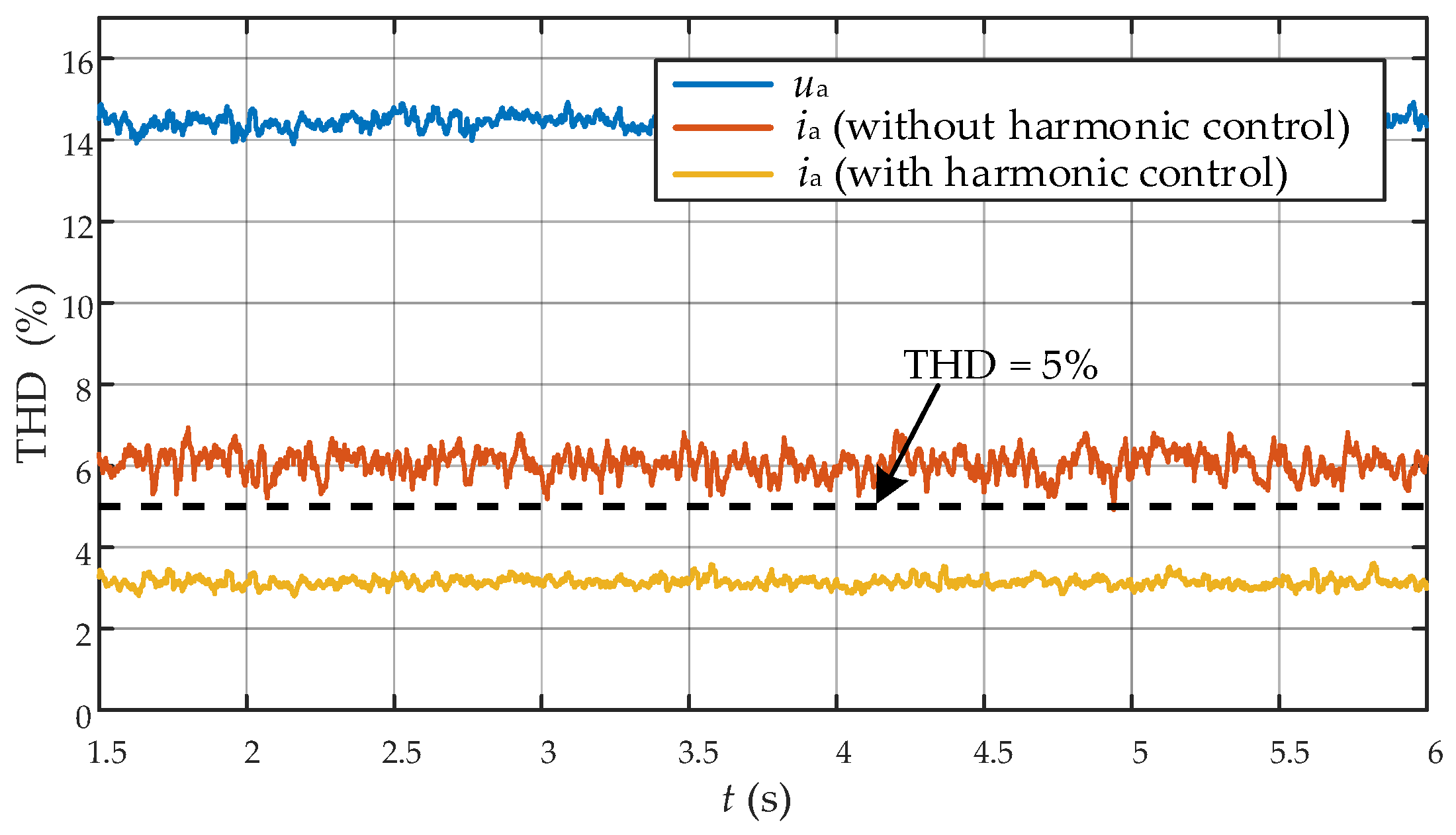
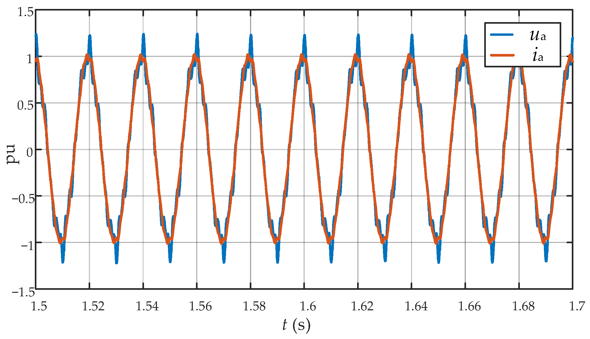
6.1. Testing Under Grid Background Harmonics Conditions

To validate the capability of the proposed strategy in reshaping current waveform quality under harmonic distortion conditions, 7% 5th, 6% 7th, 4% 11th, and 13th harmonics were injected into the ideal grid, yielding a THD of 14.5% at steady-state operation. Phase A voltage and current profiles are exemplified in Figure 20. The output current quality shows a significant improvement after the implementation of harmonic compensation. The pre-compensation THD exceeds the 5% grid code threshold, whereas the post-compensation current THD stabilizes at 3.15%. Figure 21 illustrates the relationship between regulated voltage and current at the PCC under voltage distortion conditions when using the proposed delay-compensated improved SM-MPC-QR current controller. The results reveal pronounced voltage waveform distortion that deviates from sinusoidal characteristics, while the output current maintains satisfactory sinusoidal quality.

6.2. Testing Under Grid Voltage Sag Conditions

The dynamic current amplitude reshaping performance of the proposed strategy was evaluated through unbalanced grid fault simulations, encompassing both single-phase and two-phase voltage sag scenarios. The voltage sag events were initiated at t = 2.0 s with 1.0 s duration, followed by automated voltage restoration to nominal 1.0 pu.

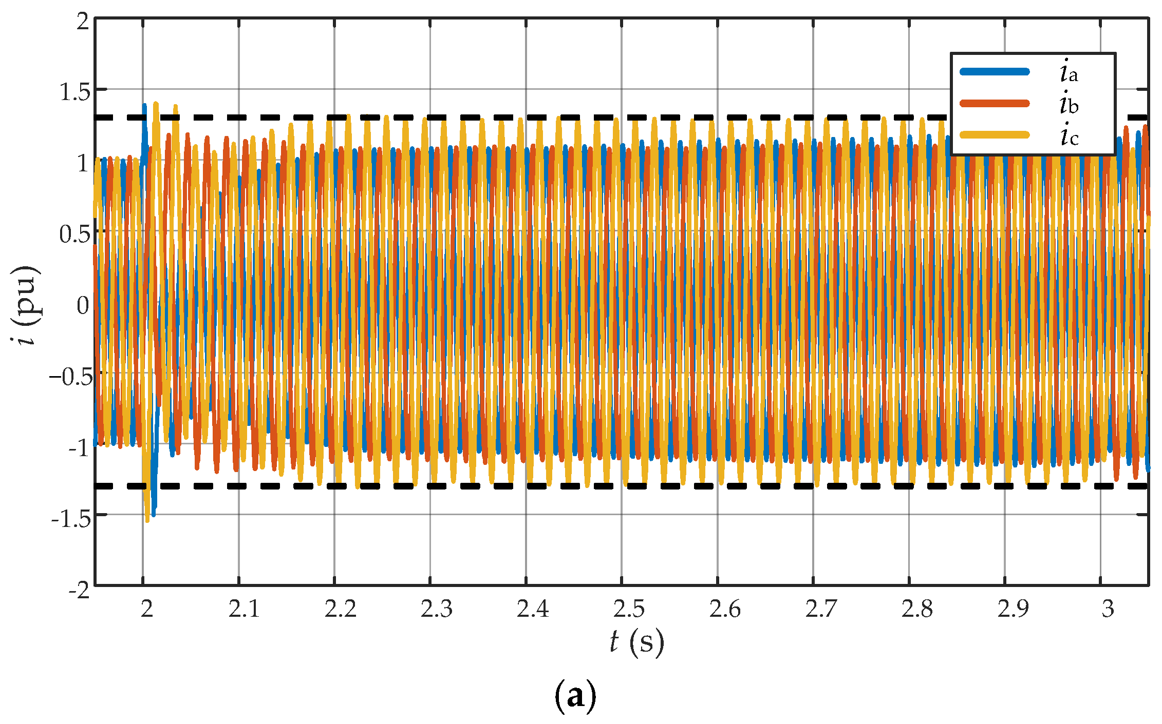
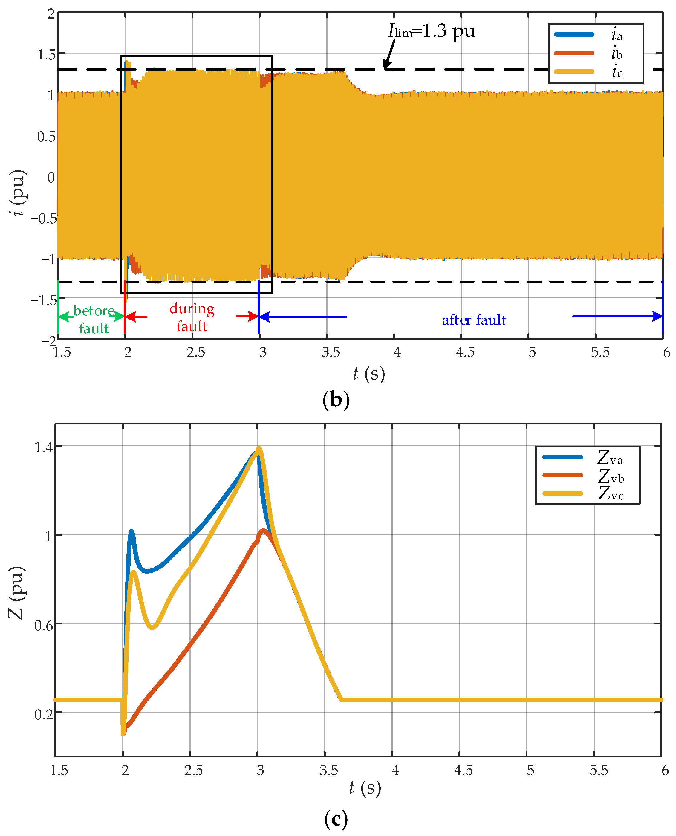
6.2.1. Single-Phase Voltage Sag Condition

The simulation results under the single-phase voltage sag of 0.9 pu are shown in Figure 22. According to the zoomed-in view in Figure 22a, it can be observed that the effect of zero sequence current is eliminated when the voltage sag occurs at the phase A voltage, and the current at the phase C is the largest, which is consistent with the theoretical results analyzed in Section Effects of Zero-Sequence Current. The maximum output current is strictly limited to 1.3 pu during steady state. As shown in Figure 22b, after voltage recovery, active power increases due to the continuous acceleration of the power angle, leading to an increase in current. Once frequency is restored to the rated value, the current returns to its rated value. Figure 22c indicates that the adaptive VI of each phase also increases instantaneously at the fault moment to suppress transient impulse overcurrent and automatically decreases after transient current suppression, aligning with the established rules of the fuzzy controller. It should be noted that the maximum VI achieved arises because the voltage sag for phase A is greater than the VI for phase C. After voltage recovery, the three-phase VI can adapt to the design specifications and gradually equalize to the steady-state value.

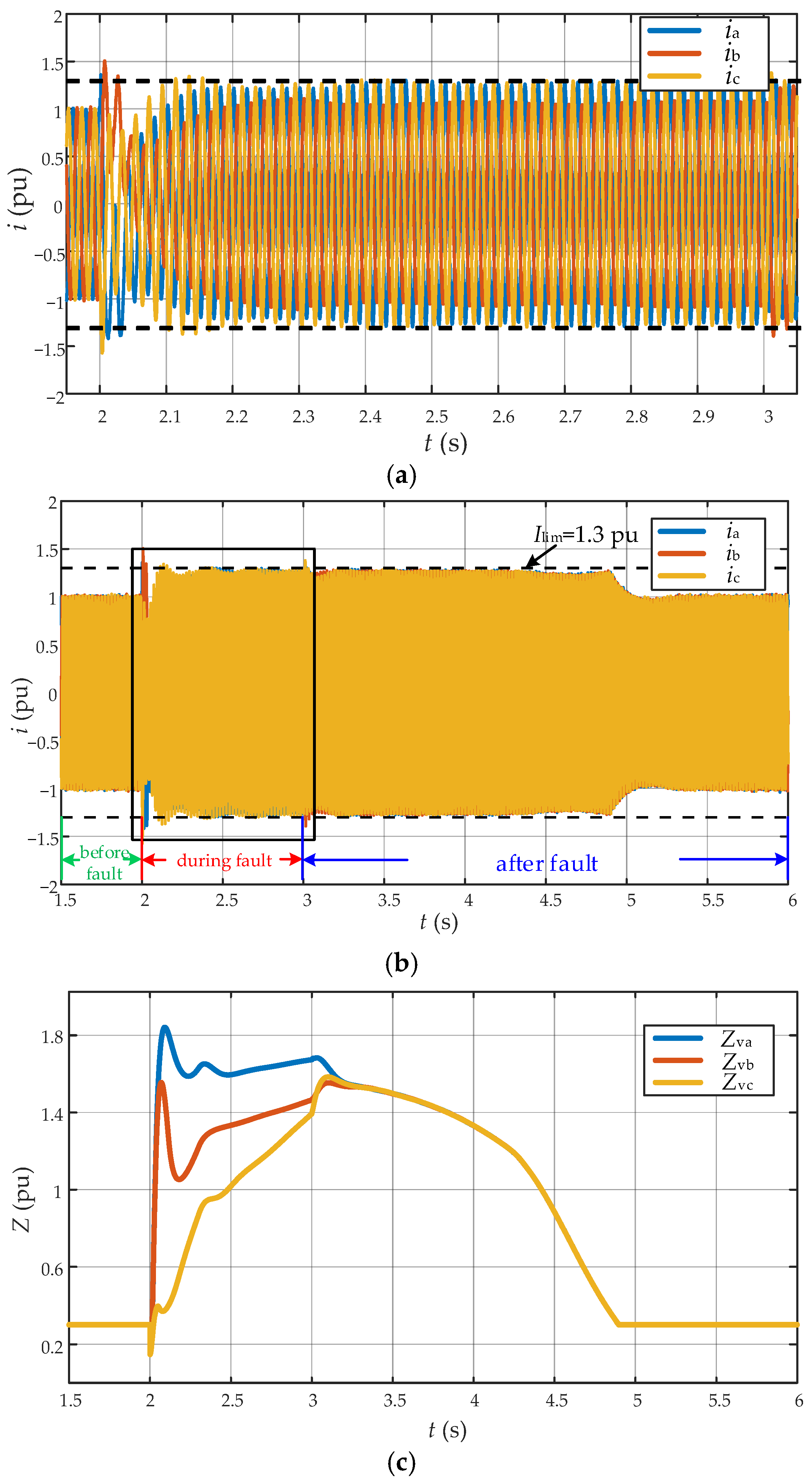
6.2.2. Two-Phase Voltage Sags Condition

The simulation results presented in Figure 23 demonstrate dynamic responses under two-phase unbalanced voltage sag conditions, specifically analyzing phase A and phase B 0.7 pu voltage depression scenarios over a duration of 1 s. Similar to single-phase sag scenarios, after zero-sequence current elimination under balanced two-phase sag conditions, the currents for phases A and C peak at 1.3 pu with effective containment. As shown in Figure 23b, three-phase currents during fault recovery exhibit higher magnitudes and prolonged stabilization durations compared to observations from single-phase cases. This stems from accelerated power angle dynamics during deeper two-phase sag events, necessitating extended frequency regulation cycles for grid resynchronization. Notably, frequency restoration to nominal value requires approximately 1.2 s longer than single-phase cases, highlighting the heightened challenges to system inertia support during multiphase faults. Figure 23c demonstrates the adaptive impedance weighting under this operating mode, validating the capability of the proposed algorithm to dynamically adjust per-phase impedance coefficients based on fault characteristics, achieving multiphase coordinated suppression. Furthermore, the adaptive strategy effectively mitigates residual imbalance effects after voltage recovery in two-phase sag scenarios.

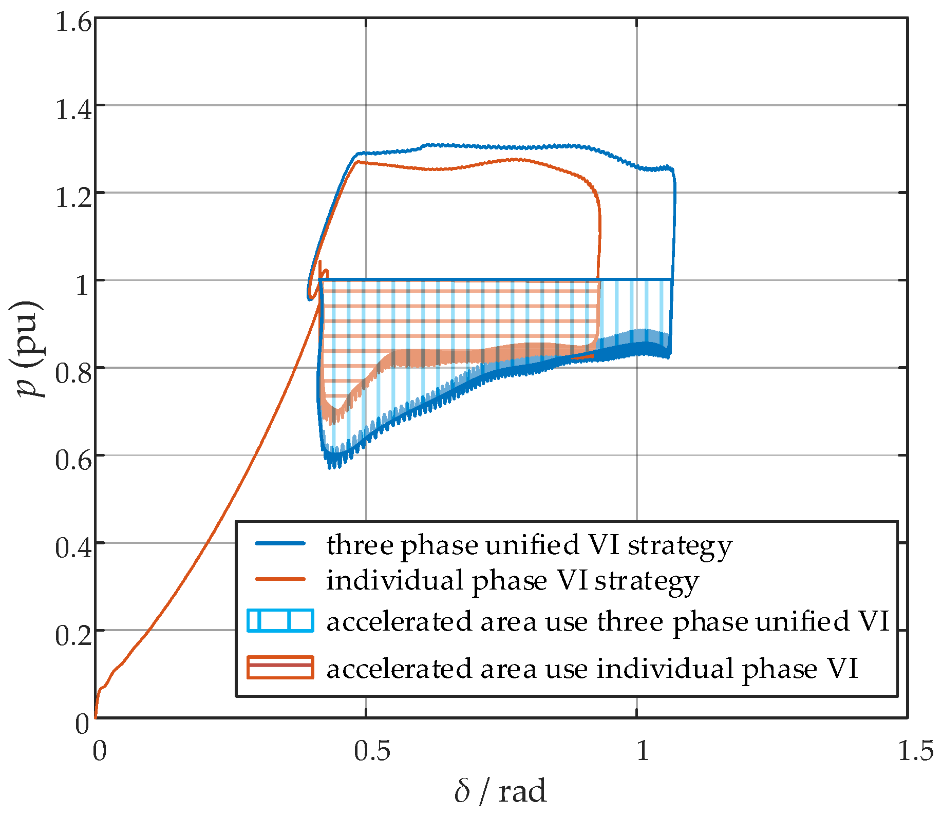
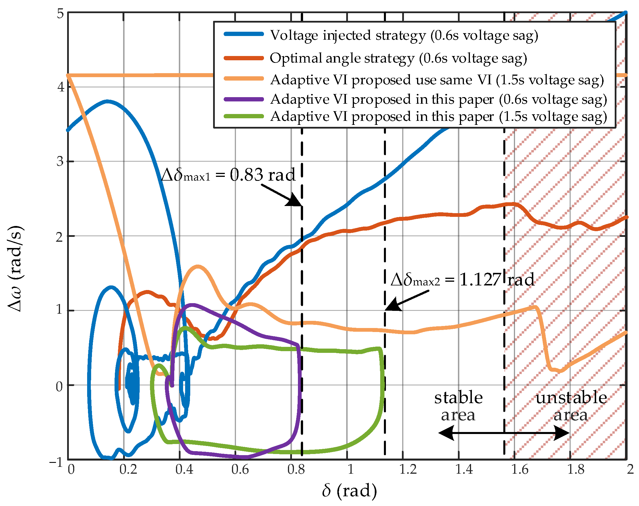
6.3. Verification of Transient Stability Improvement

Following voltage sag events, frequency deviation and power angle increase occur in the GFM due to discrepancies between active power reference and actual output values. After voltage recovery, the system can lose stability if the power angle exceeds the max critical clearing angle δ_max = 1.57 rad; otherwise, it returns to equilibrium. Transient stability performance can thus be evaluated by comparing maximum critical clearing angles across different control strategies. To validate the transient stability enhancement of the proposed adaptive VI strategy, a comparative analysis is conducted under identical conditions against the stability enhancement by using the stability enhancement strategy in [7], the stability enhancement strategy by using the optimal angle strategy in [8], and the PI-based adaptive VI method of concept 1 in [11], respectively. For intuitive visualization, the phase portrait of δ-Δω is employed for analytical evaluation. It should be noted that the corresponding methods in [7,8] are unable to achieve FRT for unbalanced faults. Therefore, we refer to the method in [42] to complement the control of the negative-sequence voltage-current loop. The PI controller parameters for voltage control loop are set as k_vp = 2.0 and k_vi = 0.5. The PI-controlled adaptive VI parameters are set as k_p = 0.1 and k_i = 25. Figure 24 illustrates phase portraits under single-phase voltage sag. As evidenced in the figure, when subjected to a voltage sag lasting 0.6 s, the power angle using the strategies from [7,8] exceeds the critical clearing angle of 1.57 rad. In contrast, the proposed adaptive VI strategy can maintain power angle stability with a maximum critical clearing angle of 0.83 rad. Under a different condition, when exposed to a 1.5 s voltage sag, the adaptive VI method presented in [11] causes the power angle to exceed the critical clearing angle, resulting in angular instability. Although post-fault voltage recovery in [7,11] enables the active power control loop to restore the rated power output, synchronous stability deteriorates during the transient resynchronization phase. In contrast, the proposed strategy demonstrates successful power angle recovery to initial stable state post-fault, achieving a maximum critical clearing angle of 1.127 rad. This enables GFM converters to maintain enhanced transient active power output while preserving transient stability.

6.4. Hardware-in-the-Loop Experiments

To validate the effectiveness of the proposed strategy, HIL testing was conducted on the Typhoon HIL platform under grid background harmonics and unbalanced voltage sag conditions. As shown in Figure 25, the HIL platform consists of a monitor, an oscilloscope, Typhoon HIL 602+, a PC, a control board, and a power quality and energy analyzer FLUKE 435 series II. The proposed strategy is implemented in digital signal processing (DSP) chip TI TMS320F28335.

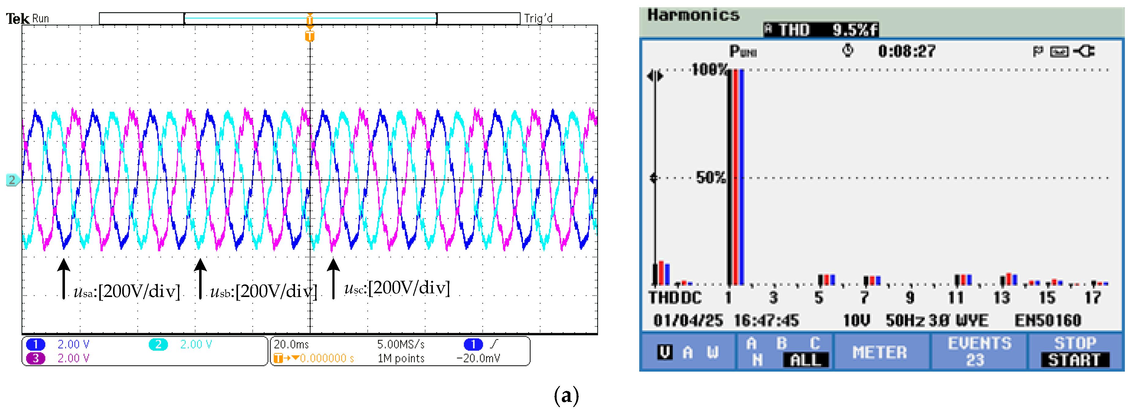
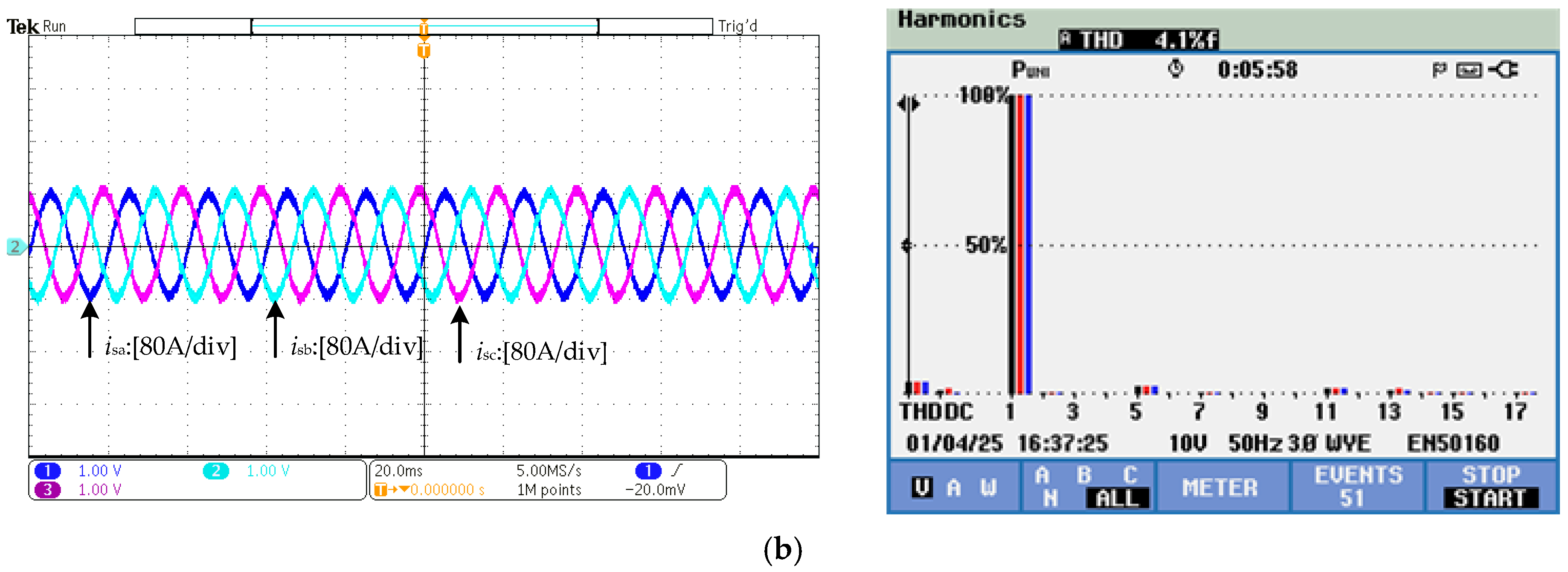
6.4.1. Test 1: Testing Under Grid Background Harmonics Conditions

To evaluate the performance and effectiveness of the proposed improved SM-MPC-QR current inner-loop control under distorted grid conditions, intentional harmonic injection was conducted with the following components: 7% 5th harmonic, 5% 7th harmonic, 1% 11th harmonic, and 1% 13th harmonic in grid voltage. Figure 26a presents the three-phase voltage waveforms and THD under harmonic injection conditions. The measured voltage THD values for phases A, B, and C, obtained from the power quality and energy analyzer, are 9.5%, 9.8%, and 9.6%, respectively, demonstrating significant deviation from ideal sinusoidal waveforms. Correspondingly, current THD measurements of 4.0%, 4.1%, and 3.8% across three phases confirm superior current quality. These results conclusively demonstrate that the proposed control strategy effectively reshapes the quality of the current waveforms and adapts to grid voltage distortion conditions. Even under severe grid voltage scenarios with THD levels approaching 10%, GFM converters maintain superior output current waveform quality while ensuring compliance with relevant standards. This experimental validation aligns with and substantiates the simulation results presented in Section 6.1.

6.4.2. Test 2: Unbalanced Grid Voltage Sag Conditions

Figure 27 and Figure 28 present experimental three-phase current profiles under voltage sag conditions: a 0.9 pu single-phase sag and a 0.7 pu two-phase sag, respectively, both with 700 ms duration. Instants t₁ and t₃ denote the initiation of the voltage sag, while t₂ and t₄ mark clearance of the sag, with the current limit threshold I_lim set at 1.3 pu. As evidenced in Figure 27, the proportional control mechanism activates instantly upon detecting a phase A sag, constraining the current surge to I_max = 1.4 pu to prevent converter overcurrent. Subsequently, the adaptive VI increases to further limit fault current through the fuzzy-integral correction module, ultimately restricting the phase current to 1.3 pu. This process maintains voltage-source characteristics in the GFM converter while leveraging the converter overload capacity to enhance current output, increase active power injection, and improve transient stability. Figure 28 validates the control robustness during a two-phase voltage sag event by demonstrating that the adaptive VI can reshape phase current amplitudes within the 1.3 pu threshold while maintaining voltage-source characteristics via dynamic reactive power compensation. Simulation results with zero-sequence components eliminated in current references demonstrate excellent agreement with theoretical analysis, both quantitatively and qualitatively.

6.4.3. Test 3: Verification of Transient Stability Improvement

To validate the transient stability enhancement of the proposed individual-phase VI control strategy, comparative experimental results with the transient stability enhancement strategies in [7,8], as well as the adaptive VI method from [11], are presented in Figure 29. Both methods were tested under identical conditions featuring a phase-A voltage sag to 0.1 pu lasting 1.02 s. Figure 29b indicates that, under the same conditions, the method proposed in [8] may lead to instability. Figure 29a,c demonstrates that although the GFM converter can restore power angle stability and resume rated active power output post-voltage recovery, transient power angle excursions exceeding 1.57 rad during dynamic adjustment processes may induce angular instability. In contrast, Figure 29d reveals that the proposed individual-phase fuzzy adaptive VI strategy enables higher active power output during and after voltage sag events, restores the power angle to steady-state values post-voltage recovery, and confirms the effectiveness of the strategy in enhancing transient stability. Experimental results exhibit excellent agreement with simulation outcomes presented in Section 6.3, demonstrating the effectiveness of the proposed strategy in enhancing transient stability of the GFM converter.

7. Discussion

In modern power systems, GFM converters have a wide range of applications due to the high penetration of renewable energy sources and extensive use of power electronics. The operational capabilities of GFM converters are particularly challenged in non-ideal grid condition characterized by voltage distortion and unbalanced sag conditions. Enhancing converter adaptability while ensuring precise current waveform regulation under these disturbances has emerged as a critical design imperative. The proposed method combines an improved SM-MPC-QR strategy with an individual-phase fuzzy integral adaptive VI strategy to improve the output power quality, limit unbalanced fault currents, and enhance the transient stability performance under non-ideal grid conditions. However, the effects of grid resistance are neglected in the analysis process, and the study of the high R/X ratio grid and different grid strength conditions is left for future research. Additionally, the adaptive VI strategy relies on a fixed X/R ratio. Subsequent studies should address variable X/R ratio conditions to further optimize the current limiting capability and transient stability performance of the GFM converter.

8. Conclusions

This article explores a novel control strategy for GFM converters that aims to reshape the current waveform and enhance transient stability, addressing the operational challenges faced by GFM converters in non-ideal grids with voltage distortions and unbalanced sags. To improve the current waveform quality of the GFM converter under grid distortion, an enhanced SM-MPC-QR current inner-loop strategy is proposed. This proposal is supported by theoretical analyses of the tracking performance and stability of the improved sliding-mode composite RL, as well as the phase lag of the quasi-resonant controller. The proposed strategy enables fast tracking of the current command while effectively suppressing harmonics under severe grid distortion. Additionally, by investigating the impact of the zero-sequence current in the reference current on current control capability and system stability, an individual-phase fuzzy-integral VI adaptive tuning strategy is proposed. This ensures that the GFM converter can maintain the ability to shape the amplitude of the controlled current waveform while exhibiting stable voltage source characteristics during grid unbalanced faults. Finally, both simulation and experimental results confirm the feasibility and effectiveness of the proposed current waveform reshaping and transient stability enhancement strategy. Compared with state-of-the-art studies, the proposed strategy can maintain the THD of the output current at 4% when the grid voltage distortion approaches 10%, while also demonstrating better transient power angle stability.

References

1. Park, J.-Y.; Chang, J.-W. Novel Autonomous Control of Grid-Forming DGs to Realize 100% Renewable Energy Grids. IEEE Trans. Smart Grid 2024, 15, 2866–2880. [Google Scholar] [CrossRef]
2. Xu, J.; Liu, W.; Liu, S.; Chang, F.; Xie, X. Current State and Development Trends of Power System Converter Grid-Forming Control Technology. Power Syst. Technol. 2022, 46, 3586–3594. [Google Scholar]
3. Eroğlu, H.; Cuce, E.; Cuce, P.M.; Gul, F.; Iskenderoğlu, A. Harmonic Problems in Renewable and Sustainable Energy Systems: A Comprehensive Review. Sustain. Energy Technol. Assess. 2021, 48, 101566. [Google Scholar] [CrossRef]
4. Hu, S.; Meng, Y.; Gong, W.; Wang, L. Operation Control Strategy of DFIG Wind Turbine Under Non-Ideal Grid Conditions. Trans. China Electrotech. Soc. 2013, 28, 99–104. [Google Scholar]
5. Taul, M.G.; Wang, X.; Davari, P.; Blaabjerg, F. Current Limiting Control with Enhanced Dynamics of Grid-Forming Converters During Fault Conditions. IEEE J. Emerg. Sel. Top. Power Electron. 2020, 8, 1062–1073. [Google Scholar] [CrossRef]
6. Martínez-Turégano, J.; Añó-Villalba, S.; Bernal-Perez, S.; Peña, R.; Blasco-Gimenez, R. Small-Signal Stability and Fault Performance of Mixed Grid Forming and Grid Following Offshore Wind Power Plants Connected to a HVDC-Diode Rectifier. IET Renew. Power Gener. 2020, 14, 2166–2175. [Google Scholar] [CrossRef]
7. Si, W.; Fang, J. Transient Stability Improvement of Grid-Forming Converters Through Voltage Amplitude Regulation and Reactive Power Injection. IEEE Trans. Power Electron. 2023, 38, 12116–12125. [Google Scholar] [CrossRef]
8. Rokrok, E.; Qoria, T.; Bruyere, A.; Francois, B.; Guillaud, X. Transient Stability Assessment and Enhancement of Grid-Forming Converters Embedding Current Reference Saturation as Current Limiting Strategy. IEEE Trans. Power Syst. 2022, 37, 1519–1531. [Google Scholar] [CrossRef]
9. Fang, J.; Si, W.; Xing, L.; Goetz, S.M. Analysis and Improvement of Transient Voltage Stability for Grid-Forming Converters. IEEE Trans. Ind. Electron. 2024, 71, 7230–7240. [Google Scholar] [CrossRef]
10. Liu, B.; Xiang, X.; Li, Y.; Yang, H.; Li, W.; He, X. Stability Constrained Transient Overcurrent Capability Enhancement of Grid Forming Converters Based on Switching Frequency Adjustment. IEEE Trans. Power Electron. 2025, 40, 2987–3004. [Google Scholar] [CrossRef]
11. Rosso, R.; Engelken, S.; Liserre, M. On the Implementation of an FRT Strategy for Grid-Forming Converters Under Symmetrical and Asymmetrical Grid Faults. IEEE Trans. Ind. Appl. 2021, 57, 4385–4397. [Google Scholar] [CrossRef]
12. GB/T 33593-2017; Technical Requirements for Grid Connection of Distributed Resources. Standardization Administration of China: Beijing, China, 2017.
13. IEEE Std 1547-2018; IEEE Standard for Interconnection and Interoperability of Distributed Energy Resources with Associated Electric Power Systems Interfaces. IEEE: Piscataway, NJ, USA, 2018.
14. Das, T.S.; Annakkage, U.D.; Muthumuni, D.; Park, I.K. Robust higher order sliding mode control of grid-forming converters with LCL filter in weak grid scenarios for fast frequency support. IET Gener. Transm. Distrib. 2024, 18, 3851–3862. [Google Scholar] [CrossRef]
15. Fu, C.; Zhang, C.; Zhang, G.; Zhang, C.; Su, Q. Finite-Time Command Filtered Control of Three-Phase AC/DC Converter Under Unbalanced Grid Conditions. IEEE Trans. Ind. Electron. 2023, 70, 6876–6886. [Google Scholar] [CrossRef]
16. Komurcugil, H.; Biricik, S.; Bayhan, S.; Zhang, Z. Sliding Mode Control: Overview of Its Applications in Power Converters. IEEE Ind. Electron. Mag. 2021, 15, 40–49. [Google Scholar] [CrossRef]
17. Wang, Z.; Li, S.; Li, Q. Discrete-Time Fast Terminal Sliding Mode Control Design for DC–DC Buck Converters with Mismatched Disturbances. IEEE Trans. Ind. Inform. 2020, 16, 1204–1213. [Google Scholar] [CrossRef]
18. Pal, A.; Hosseinabadi, P.A.; Panigrahi, B.K.; Pota, H.R. A Fixed-Time Sliding Mode Controller for Black-Starting of Grid-Forming Inverter-Based Generations. In Proceedings of the 2024 IEEE 4th International Conference on Sustainable Energy and Future Electric Transportation (SEFET), Hyderabad, India, 31 July–3 August 2024; pp. 1–5. [Google Scholar]
19. Haroon, F.; Aamir, M.; Waqar, A.; Qaisar, S.M.; Ali, S.U.; Almaktoom, A.T. A Composite Exponential Reaching Law Based SMC with Rotating Sliding Surface Selection Mechanism for Two Level Three Phase VSI in Vehicle to Load Applications. Energies 2023, 16, 346. [Google Scholar] [CrossRef]
20. Jeeranantasin, N.; Nungam, S. Sliding Mode Control of Three-Phase AC/DC Converters Using Exponential Rate Reaching Law. J. Syst. Eng. Electron. 2022, 33, 210–221. [Google Scholar] [CrossRef]
21. Ye, T.; Dai, N.; Lam, C.-S.; Wong, M.-C.; Guerrero, J.M. Analysis, Design and Implementation of a Quasi-Proportional-Resonant Controller for a Multifunctional Capacitive-Coupling Grid-Connected Inverter. IEEE Trans. Ind. Appl. 2016, 52, 4269–4280. [Google Scholar] [CrossRef]
22. Mishra, M.K.; Lal, V.N. An Advanced Proportional Multiresonant Controller for Enhanced Harmonic Compensation with Power Ripple Mitigation of Grid-Integrated PV Systems Under Distorted Grid Voltage Conditions. IEEE Trans. Ind. Appl. 2021, 57, 5318–5331. [Google Scholar] [CrossRef]
23. Hans, F.; Schumacher, W.; Chou, S.-F.; Wang, X. Design of Multifrequency Proportional–Resonant Current Controllers for Voltage-Source Converters. IEEE Trans. Power Electron. 2020, 35, 13573–13589. [Google Scholar] [CrossRef]
24. Qoria, T.; Gruson, F.; Colas, F.; Denis, G.; Prevost, T.; Guillaud, X. Critical Clearing Time Determination and Enhancement of Grid-Forming Converters Embedding Virtual Impedance as Current Limitation Algorithm. IEEE J. Emerg. Sel. Top. Power Electron. 2020, 8, 1050–1061. [Google Scholar] [CrossRef]
25. Jin, Z.; Wang, X. A DQ-Frame Asymmetrical Virtual Impedance Control for Enhancing Transient Stability of Grid-Forming Inverters. IEEE Trans. Power Electron. 2022, 37, 4535–4544. [Google Scholar] [CrossRef]
26. Zhou, L.; Liu, S.; Chen, Y.; Yi, W.; Wang, S.; Zhou, X. Harmonic Current and Inrush Fault Current Coordinated Suppression Method for VSG Under Non-Ideal Grid Condition. IEEE Trans. Power Electron. 2021, 36, 1030–1042. [Google Scholar] [CrossRef]
27. Baeckeland, N.; Venkatramanan, D.; Kleemann, M.; Dhople, S. Stationary-Frame Grid-Forming Inverter Control Architectures for Unbalanced Fault-Current Limiting. IEEE Trans. Energy Convers. 2022, 37, 2813–2825. [Google Scholar] [CrossRef]
28. Narula, A.; Imgart, P.; Bongiorno, M.; Beza, M.; Svensson, J.R.; Hasler, J.-P. Voltage-Based Current Limitation Strategy to Preserve Grid-Forming Properties Under Severe Grid Disturbances. IEEE Open J. Power Electron. 2023, 4, 176–188. [Google Scholar] [CrossRef]
29. Mahamedi, B.; Eskandari, M.; Fletcher, J.E.; Zhu, J. Sequence-Based Control Strategy with Current Limiting for the Fault Ride-Through of Inverter-Interfaced Distributed Generators. IEEE Trans. Sustain. Energy 2020, 11, 165–174. [Google Scholar] [CrossRef]
30. Jia, Q.; Liu, J.; Liu, J.; Xu, J. A General Current Limiting Strategy of Grid-Forming Converters Based on Adaptive Virtual Impedance Regulated by Fuzzy PI Control. In Proceedings of the 2024 IEEE 10th International Power Electronics and Motion Control Conference (IPEMC2024-ECCE Asia), Chengdu, China, 17–20 May 2024; pp. 4836–4841. [Google Scholar]
31. Sebaaly, F.; Vahedi, H.; Kanaan, H.Y.; Moubayed, N.; Al-Haddad, K. Sliding Mode Fixed Frequency Current Controller Design for Grid-Connected NPC Inverter. IEEE J. Emerg. Sel. Top. Power Electron. 2016, 4, 1397–1405. [Google Scholar] [CrossRef]
32. Zhao, S.; Shao, B.; Gao, B.; Li, R.; Pei, J. Sliding Mode Current Control Design and Stability Analysis of VSC-HVDC Based on Combinatorial Reaching Law. High Volt. Eng. 2019, 45, 3603–3611. [Google Scholar]
33. Liu, J. Sliding Mode Control Design and MATLAB Simulation: The Basic Theory and Design Method, 3rd ed.; Tsinghua University Press: Beijing, China, 2015. [Google Scholar]
34. Qiao, Z.; Shi, T.; Wang, Y.; Yan, Y.; Xia, C.; He, X. New Sliding-Mode Observer for Position Sensorless Control of Permanent-Magnet Synchronous Motor. IEEE Trans. Ind. Electron. 2013, 60, 710–719. [Google Scholar] [CrossRef]
35. Sarpturk, S.; Istefanopulos, Y.; Kaynak, O. On the Stability of Discrete-Time Sliding Mode Control Systems. IEEE Trans. Autom. Control 1987, 32, 930–932. [Google Scholar] [CrossRef]
36. Li, T.; Li, Y.; Li, S.; Zhang, W. Research on Current-Limiting Control Strategy Suitable for Ground Faults in AC Microgrid. IEEE J. Emerg. Sel. Top. Power Electron. 2021, 9, 1736–1750. [Google Scholar] [CrossRef]
37. Yepes, A.G.; Freijedo, F.D.; Doval-Gandoy, J.; López, Ó.; Malvar, J.; Fernandez-Comesaña, P. Effects of Discretization Methods on the Performance of Resonant Controllers. IEEE Trans. Power Electron. 2010, 25, 1692–1712. [Google Scholar] [CrossRef]
38. Zhao, F.; Zhu, T.; Harnefors, L.; Fan, B.; Wu, H.; Zhou, Z. Closed-Form Solutions for Grid-Forming Converters: A Design-Oriented Study. IEEE Open J. Power Electron. 2024, 5, 186–200. [Google Scholar] [CrossRef]
39. Zhang, Y.; Zhang, C.; Yang, R.; Molinas, M.; Cai, X. Current-Constrained Power-Angle Characterization Method for Transient Stability Analysis of Grid-Forming Voltage Source Converters. IEEE Trans. Energy Convers. 2023, 38, 1338–1349. [Google Scholar] [CrossRef]
40. Rodriguez, P.; Candela, I.; Citro, C.; Rocabert, J.; Luna, A. Control of Grid-Connected Power Converters Based on a Virtual Admittance Control Loop. In Proceedings of the 15th European Conference on Power Electronics and Applications (EPE), Lille, France, 2–6 September 2013; pp. 1–10. [Google Scholar]
41. Cai, S.; Liang, D.; Zhou, K.; Zhang, L.; Liu, Y. Switching Strategy with the Improved Single-Phase dq0 Voltage Detection Method for the Load Voltage Compensation Unit of Hybrid Distribution Transformer. Trans. China Electrotech. Soc. 2021, 36, 126–132. [Google Scholar]
42. Tavakoli, S.D.; Prieto-Araujo, E.; Gomis-Bellmunt, O.; Galceran-Arellano, S. Fault ride-through control based on voltage prioritization for grid-forming converters. IET Renew. Power Gener. 2023, 17, 1370–1384. [Google Scholar] [CrossRef]
Figure 1. Topology and Control Strategies of GFM.
Energies 18 02834 g001
Figure 2. Improved combinatorial reaching law composition function. (a) Arccot (|s|) function waveform; (b) Comparison of improved sign functions.
Energies 18 02834 g002
Figure 3. Improved convergence performance comparison of combinatorial reaching law.
Energies 18 02834 g003
Figure 4. The compensation strategy of the improved quasi-resonant controller.
Energies 18 02834 g004
Figure 5. Control block diagram of PC-QR controller.
Energies 18 02834 g005
Figure 6. Open-loop system bode diagram.
Energies 18 02834 g006
Figure 7. Closed-loop system bode diagram.
Energies 18 02834 g007
Figure 8. Current control loop incorporating delay-compensated improved quasi-resonant strategy.
Energies 18 02834 g008
Figure 9. PC-QR strategy considering digital control delay compensation.
Energies 18 02834 g009
Figure 10. Bode diagram of phase-compensated system.
Energies 18 02834 g010
Figure 11. Control block diagram of the improved SM-MPC-QR current inner-loop.
Energies 18 02834 g011
Figure 12. Design of fuzzy-based correction module.
Energies 18 02834 g012
Figure 13. The design of the fuzzy controller. (a) Membership function curves of input efuzzy; (b) Membership function curves of input defuzzy; (c) Membership function curves of output kvi; (d) Input–output relationship.
Energies 18 02834 g013
Figure 14. Simulation result using the same k and VI. (a) Current waveform; (b) P-δ curve.
Energies 18 02834 g014
Figure 15. Space vector diagram under phase A voltage sag condition.
Energies 18 02834 g015
Figure 16. Simulation result using same VI with zero-sequence separation.
Energies 18 02834 g016
Figure 17. Individual phase VI strategy through zero-sequence current separation.
Energies 18 02834 g017
Figure 18. Comparation of P-δ curves with and without phase separation control.
Energies 18 02834 g018
Figure 19. Overall strategy control block diagram.
Energies 18 02834 g019
Figure 20. THD of voltage and current.
Energies 18 02834 g020
Figure 21. Voltage-current relationship under voltage distortion.
Energies 18 02834 g021
Figure 22. Simulation results of Phase A voltage sag. (a) Zoomed in view of current waveforms; (b) Current waveforms; (c) Adaptive VI for individual phase.
Energies 18 02834 g022aEnergies 18 02834 g022b
Figure 23. Simulation results of AB two-phase voltage sags. (a) Zoomed in view of current waveforms; (b) Current waveforms; (c) Adaptive VI for individual phase.
Energies 18 02834 g023
Figure 24. Phase portrait of δω comparison of existing advanced transient stability enhancement method under single-phase voltage sag (blue line refers to strategy in [7], red line refers to strategy in [8], yellow line refers to strategy in [11], purple and green lines refer to strategy in this paper).
Energies 18 02834 g024
Figure 25. Experimental setup.
Energies 18 02834 g025
Figure 26. The waveforms and frequency spectrums of three-phase voltages and currents under distorted grid voltages. (a) Waveforms and frequency spectrums of voltages; (b) Waveforms and frequency spectrums of currents.
Energies 18 02834 g026aEnergies 18 02834 g026b
Figure 27. Three-phase current dynamics during single phase (A) voltage sag.
Energies 18 02834 g027
Figure 28. Three-phase current dynamics during two-phase (AB) voltage sag.
Energies 18 02834 g028
Figure 29. Experimental waveforms when the voltage of phase A sag. (a) Using stability enhancement strategy in [7]; (b) Using optimal angle strategy in [8]; (c) Using adaptive VI strategy in [11]; (d) Using proposed individual phase VI strategy.
Energies 18 02834 g029aEnergies 18 02834 g029b