Diffusion Modeling of Carbon Dioxide Concentration from Stationary Sources with Improved Gaussian Plume Modeling

Abstract

To achieve the precise quantification and real-time monitoring of CO₂ emissions from stationary sources, this study developed a Gaussian plume model-based dispersion framework incorporating emission characteristics. Critical factors affecting CO₂ dispersion were systematically analyzed, with model optimization conducted through plume rise height adjustments and reflection coefficient calibrations. MATLAB-based simulations on an industrial park case study demonstrated that wind speed, atmospheric stability, and effective release height constituted pivotal determinants for enhancing CO₂ dispersion modeling accuracy. Furthermore, the inverse estimation of source strength at emission terminals was implemented via particle swarm optimization, establishing both theoretical foundations and methodological frameworks for the precision monitoring and predictive dispersion analysis of stationary-source CO₂ emissions.

1. Introduction

As one of the world’s major carbon dioxide emitters, China is resolutely implementing its “dual-carbon” goals to address global climate change [1,2]. The power sector is one of the primary contributors to carbon dioxide emissions, with CO₂ from fossil fuel combustion in thermal power plants being a critical factor driving high carbon emissions in the electricity industry [3,4].

Common gas diffusion models can be categorized into Lagrangian diffusion models, Eulerian diffusion models, and Gaussian diffusion models [5,6]. The Gaussian diffusion model, serving as an empirical framework for studying light gas dispersion patterns, possesses the capability to handle fuzziness and stochasticity, functioning as a mathematical tool for transforming qualitative concepts into quantitative values [7]. Shi Baojun et al. [8] conducted in-depth analysis of LPG leakage dispersion patterns using a Gaussian plume hybrid model, identifying wind speed, atmospheric stability, and surface roughness as critical influencing factors. Liu Yongmin et al. [9] employed the Gaussian model to investigate the dispersion patterns of converter gas emissions through tall chimneys under varying atmospheric stability and wind speed conditions. Wang Hongde et al. [10] explored the leakage and diffusion patterns of liquid ammonia storage tanks using the Gaussian plume model. Zheng Hongbo et al. [11] developed a visual analytical method for waste incineration plant emissions based on the Gaussian diffusion model, achieving the real-time monitoring of exhaust pollutants. Chen Jutao [12] implemented the dynamic simulation of ship gas dispersion in Xiamen Port through Web GIS integration with Gaussian line-source atmospheric dispersion modeling. Lu Shijian et al. [13] investigated nitrosamine concentration gradients in absorber tail gas using Gaussian modeling, concluding that an 83% emission reduction at the absorber top achieved an acceptable carcinogenic risk level of 10⁻⁶. Zhang et al. [14] predicted radionuclide volume fractions using an optimized Gaussian dispersion model. Pournazeri et al. [15] proposed a numerical plume rise model accounting for building-induced flows and evaluated its urban applicability. Chen et al. [16] developed a refined Gaussian plume model demonstrating the accurate prediction of gaseous pollutant concentration distributions. Yuval et al. [17] created a novel nonlinear air quality regression model based on Gaussian dispersion theory to elucidate spatial pollution–health outcome relationships. European and American researchers validated CO₂-CEMS accuracy in stationary emission sources by analyzing multiple thermal power plants, revealing a <3% overall discrepancy between CEMS and calculation methods. However, significant plant-level variations were observed: 50% exceeded a 5% deviation, with 20% surpassing 10% [18]. Despite technological advancements in gas monitoring, ensuring CEMS adaptability remains crucial due to prolonged exposure to high-temperature and high-humidity environments. Zhu [19] enhanced CEMS accuracy by investigating sampling losses under varied conditions, establishing particle deposition velocities through numerical solutions of transport equations along sampling lines. YHULL [10] proposed a method coupling continuous CEMS analyzers with predictive deterministic values to improve data accuracy during system bridging downtime.

In existing dispersion models, the Gaussian plume model is suitable for flat terrain or steady meteorological conditions, neglecting terrain undulations’ effects on airflow (e.g., valley effects and ridge bypass flows) [20]; it employs static reflection coefficients, failing to capture dynamic changes in surface albedo (such as diurnal temperature variations and seasonal vegetation coverage changes). Although the Lagrangian model can simulate dispersion processes by tracking virtual particle trajectories and can partially capture turbulence effects, its high computational costs hinder its applications to complex terrains and large spatial scales; a reliance on empirical turbulence parameterization schemes leads to significantly increased errors under strong convection or temperature inversion conditions. CFD (computational fluid dynamics) accurately simulates flow fields based on Navier–Stokes equations, applicable to small-scale complex terrains. However, its requirement for high-resolution terrain and meteorological data makes practical data acquisition challenging [21], while neglecting dynamic reflection mechanisms in the atmospheric boundary layer (e.g., feedback effects of surface thermal radiation on dispersion pathways). Current research remains inadequate in validating the impact mechanisms of stationary CO₂ emissions through experimental data. Ambiguities persist regarding gas diffusion model selection across diverse environments, particularly in industrial parks where large-scale monitoring systems generate massive CO₂ data throughput that exceeds the capacity of conventional data service technologies to ensure efficient and reliable transmission. This necessitates developing distributed data service architectures for CO₂ concentration detection to ensure data validity and information credibility [22].

This study established a CO₂ dispersion concentration prediction model for stationary sources using Gaussian plume modeling, systematically investigating spatiotemporal distribution patterns and dominant influencing factors through parameter sensitivity analysis and optimization methods. Selecting a representative industrial park as the case study, multi-scenario numerical simulations conducted on MATLAB R2023a revealed that horizontal wind speed, atmospheric stability, and effective emission height significantly regulated spatial heterogeneity in near-surface CO₂ concentration fields. Building upon this framework, we innovatively integrated particle swarm optimization (PSO) into an inverse modeling architecture to develop a source intensity inversion model. This advancement enabled the dynamic resolution of CO₂ emission rates at stationary-source outlets, demonstrating superior accuracy compared to conventional inversion methods. The findings provide scientific foundations for precise carbon monitoring, dispersion simulation, and emission inventory verification in industrial parks, offering theoretical and practical guidance for enhancing regional carbon footprint assessment systems.

2. Methodology

2.1. Stationary-Source CO₂ Dispersion Model and Its Optimization

Carbon dioxide emissions from stationary sources are emissions from planned and designed stationary sources at industrial facilities or from other human activities. In the case of thermal power plants, stationary-source emissions are defined as the regular emission of carbon dioxide into the atmosphere from fixed exhaust outlets such as stacks and the exhaust stacks of production units [23]. The model predictions and field measurements are also compared, as shown in

Table 1. Comparison of field measurements and model predictions.

Characterization	On-site Measurement	Model Prediction	Value of Synergies
Space Coverage	Dependence on sensor deployment density	Continuous coverage throughout the region	Model fills in gaps in sensor-sparse regions
Time Resolution	Dependent on sampling frequency (minutes/hours)	Real-time/on-demand simulation	The model provides continuous dynamic data flow
Costs	High (equipment, maintenance, manpower)	Low (one-time development, double counting)	Reduced number of sensors (cost reduction)
Applicable Scenarios	Reachable area, validation monitoring	Hazardous/inaccessible areas, predictive warning	Models guide the optimal deployment of sensors

.

The Gaussian plume model is a commonly used gas diffusion model that can be used to simulate the diffusion and concentration distribution of gaseous pollutants in the atmosphere. It is suitable for small- to medium-scale use and uniformly continuous emission sources. Assuming that the carbon dioxide emission source is an elevated point source, the carbon dioxide emission from the elevated point source of a thermal power plant is simulated and predicted based on the Gaussian plume model [23]. The following conditions need to be met for the Gaussian smoke plume model to be used:

Uniform and stable wind speed and direction in the region;

The source strength is uniformly continuous and consistent;

Atmospheric stability is described through stability categories (e.g., A, B, C, D, etc.);

The gas concentration distribution on the Y- and Z-axes satisfies a Gaussian distribution.

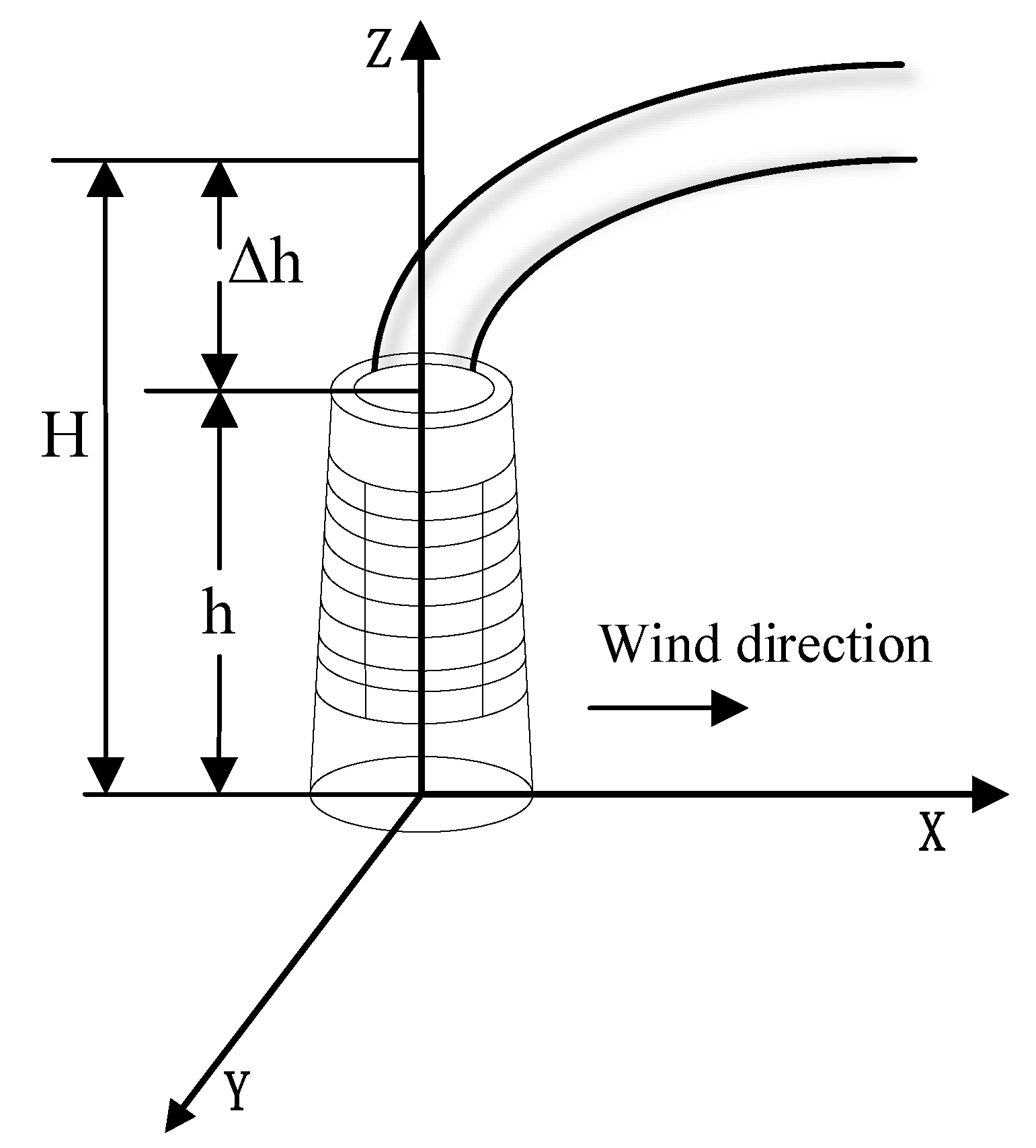
Under these conditions, we employ the Gaussian plume model to simulate CO₂ concentration distribution, assuming a homogeneous medium and constant emission rate. The estimation of carbon dioxide dispersion is achieved by calculating propagation ranges in vertical and horizontal directions from fixed emission sources, while incorporating factors including emission rate, wind speed, and stability categories. The fixed source is defined as the coordinate origin with the positive X-axis aligned with the downwind direction [24]. The Y-axis is perpendicular to the X-axis in the horizontal plane (positive direction to the left of the X-axis), and the Z-axis extends vertically upward from the horizontal plane, as illustrated in Figure 1.

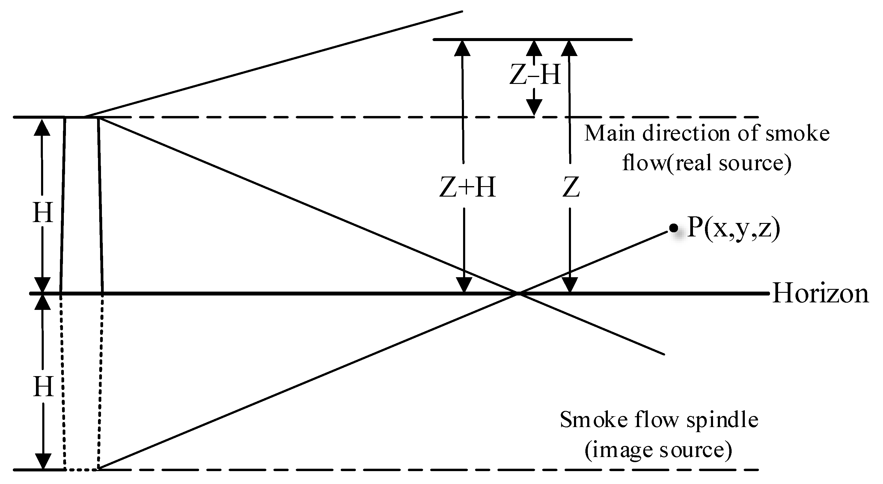
Stationary sources are generally elevated point sources where the point source is located high above the ground surface; since the dispersion of pollutants in the vertical direction is affected by the ground, this ground effect needs to be taken into account through boundary conditions. Therefore, mirror sources [25] are introduced to satisfy the boundary conditions, as shown in Figure 2.

The real source contribution value is $C_1$ by the mirror method [26]:

$$C_1(x,y,z,H)={\displaystyle \frac{Q}{2\pi u{\sigma }_y{\sigma }_z}}\exp (-{\displaystyle \frac{y^2}{2{\sigma }_y^2}})\exp (-{\displaystyle \frac{{(z-H)}^2}{2{\sigma }_z^2}})$$

(1)

The reflected image source contribution is $C_2$:

$$C_2(x,y,z,H)={\displaystyle \frac{Q}{2\pi u{\sigma }_y{\sigma }_z}}\exp (-{\displaystyle \frac{y^2}{2{\sigma }_y^2}})\exp (-{\displaystyle \frac{{(z+H)}^2}{2{\sigma }_z^2}})$$

(2)

Actual concentration $C$:

$$C(x,y,z,H)=C_1(x,y,z,H)+C_2(x,y,z,H)$$

(3)

$$\begin{array}{l}C(x,y,z,H)={\displaystyle \frac{Q}{2\pi u{\sigma }_y{\sigma }_z}}\times \\ \exp (-{\displaystyle \frac{y^2}{2{\sigma }_y^2}})\left[\exp (-{\displaystyle \frac{1}{2}}{\displaystyle \frac{{\left(z-H\right)}^2}{{\sigma }_z^2}})+\exp (-{\displaystyle \frac{1}{2}}{\displaystyle \frac{{\left(z+H\right)}^2}{{\sigma }_z^2}})\right]\end{array}$$

(4)

where $C(x,y,z,H)$ is the concentration of pollutant at any point in space (g/m³); $Q$ is the source strength of CO₂ emissions from stationary sources (g/s); $u$ is the wind speed (m/s); ${\sigma }_y$ is the diffusion coefficient in the upwind direction in the horizontal direction (m); ${\sigma }_z$ is the diffusion coefficient in the upwind direction in the vertical direction (m); and $H$ is the height of CO₂ emission source (m).

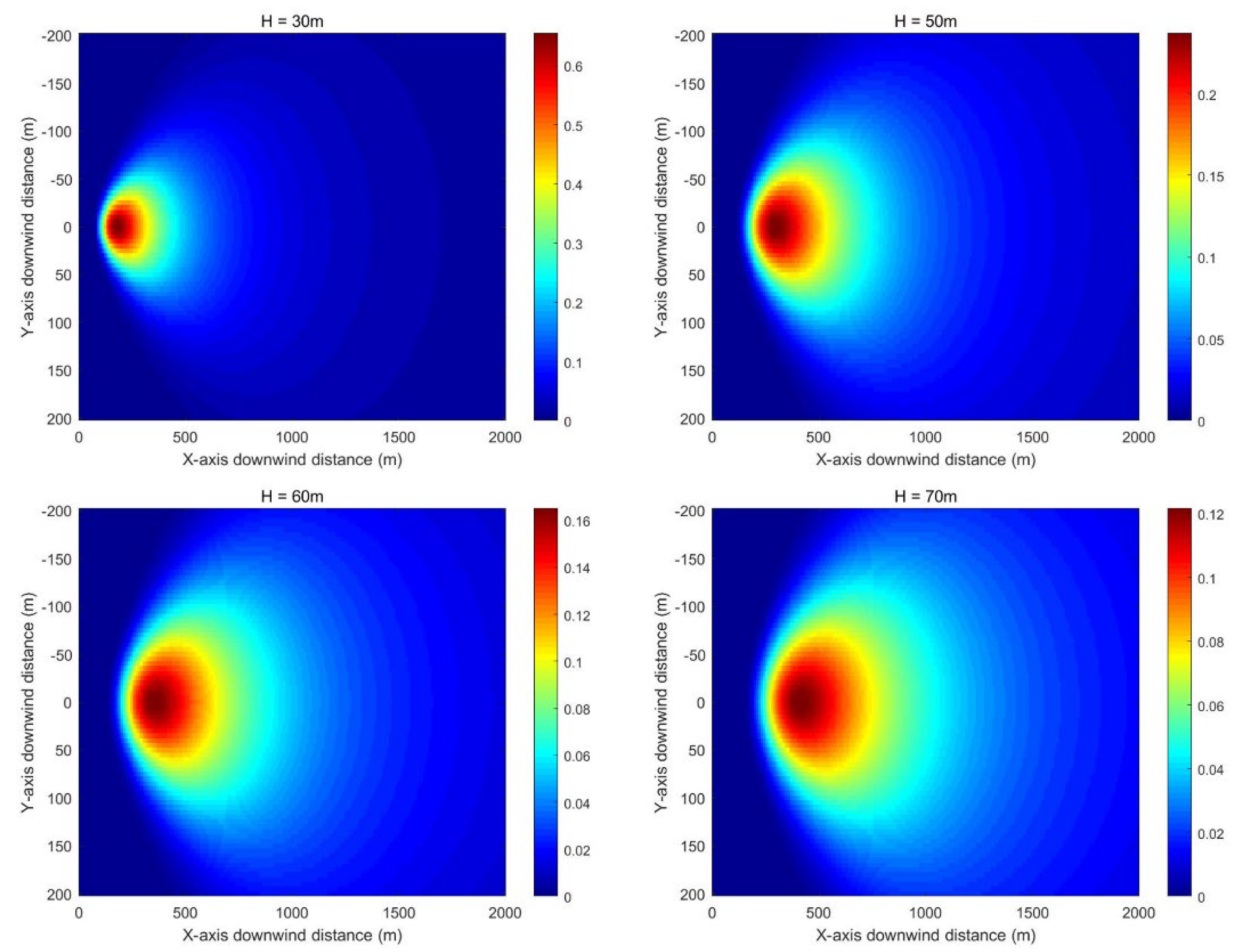
The effective height of the actual CO₂ emission source $H$ consists of the stack height $h$ and the flue gas lift height $\Delta h$ and is calculated using the following formula:

$$H=h+\Delta h$$

(5)

The height of flue gas lift has a significant effect on CO₂ diffusion, and the equation is as follows:

$$\Delta h={\displaystyle \frac{v_{s}D}{\overline{u}}}(1.5+2.7{\displaystyle \frac{T_s-T_a}{T_s}}D)={\displaystyle \frac{1}{\overline{u}}}(1.5v_{s}D+9.6\times {10}^{-3}{Q}_H)$$

(6)

where $v_s$ is the concentration of pollutants (g/m³); $D$ is the inner diameter of the chimney outlet (m); $T_s$ is the temperature of the flue gas outlet (K); $T_a$ is the average temperature of the ambient atmosphere (K); $Q_H$ is the heat emission rate of the chimney (KW); and $\overline{u}$ is the average wind speed at the chimney outlet (m/s).

Plume rise height is also influenced by atmospheric stability. Plumes tend to rise more readily under unstable conditions, while plume rise may be constrained under stable or temperature inversion conditions. These factors must be incorporated when applying Gaussian dispersion models to ensure that prediction results closely approximate real-world scenarios [27]. This demonstrates that calculating plume rise height is computationally intensive and challenging; therefore, empirical formulas can be considered to simplify the calculations. The specific methods are summarized in

Table 2. Empirical formulas for plume rise height.

Actual Height of Stationary-Source Chimney $\mathit{h}$(m)	Plume Rise Height $\Delta \mathit{h}$(m)
h ≥ 50	15
50 > h ≥ 30	8
h < 30	5

.

When z equals 0, it is considered to represent the ground-level CO₂ concentration within the industrial park. For CO₂ or any gaseous pollutant, ground-level concentration serves as the most direct and critical indicator for assessing their impacts on human activities and environmental effects at the surface. The ground-level CO₂ concentration distribution across the industrial park can be derived as follows:

$$C(x,y,0,H)={\displaystyle \frac{Q}{2\pi u{\sigma }_y{\sigma }_z}}\times \exp (-{\displaystyle \frac{y^2}{2{\sigma }_y^2}}-{\displaystyle \frac{H^2}{2{\sigma }_z^2}})$$

(7)

Similarly, when y = 0 and z = 0, this represents the pollutant concentration distribution along the central axis downwind of the stack at ground level. Analyzing this scenario allows for the evaluation of maximum ground-level concentrations at the downwind locations most likely to expose human populations to the pollutant, providing data support for pollution prevention and control measures in industrial parks. The calculation formula for ground-level axial gas concentration is expressed as follows:

$$C(x,0,0,H)={\displaystyle \frac{Q}{\pi u{\sigma }_y{\sigma }_z}}\times \exp (-{\displaystyle \frac{H^2}{2{\sigma }_z^2}})$$

(8)

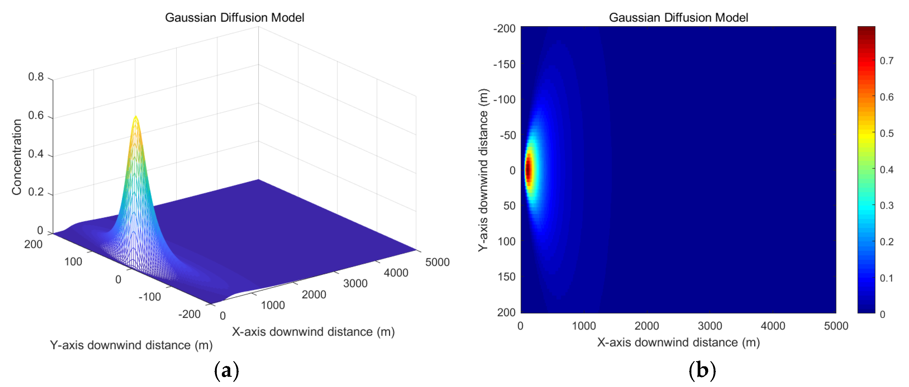
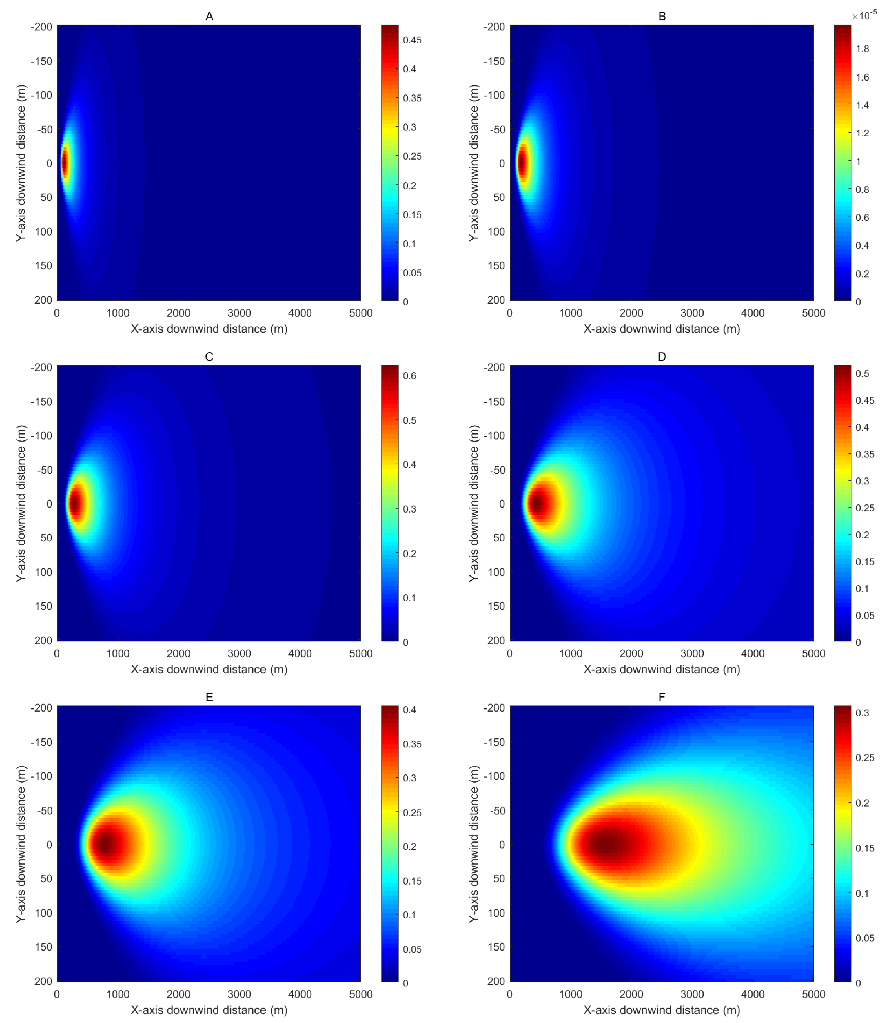
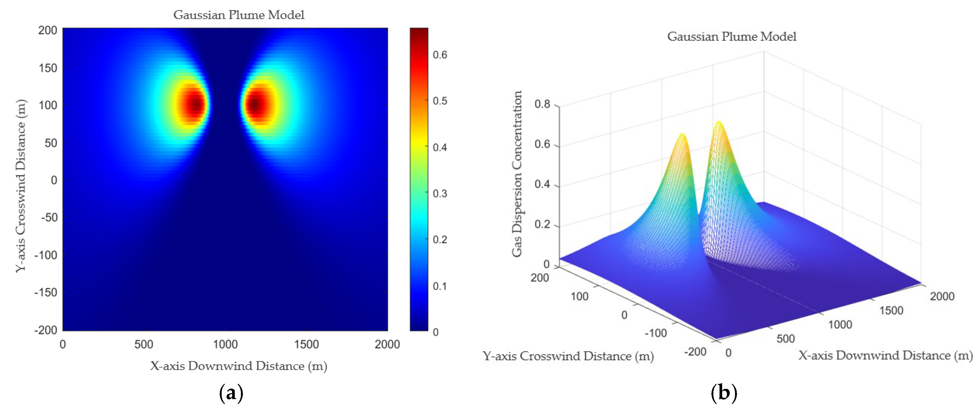
A simplified simulation of the stationary-source CO₂ dispersion model is implemented in MATLAB, with the source strength set to 10,000 g/s, effective stack height to 30 m, and wind speed u to 3 m/s. The simulation yields the results shown in Figure 3.

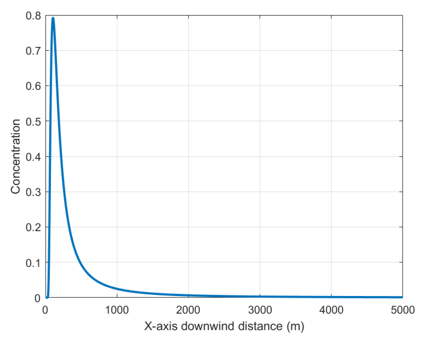
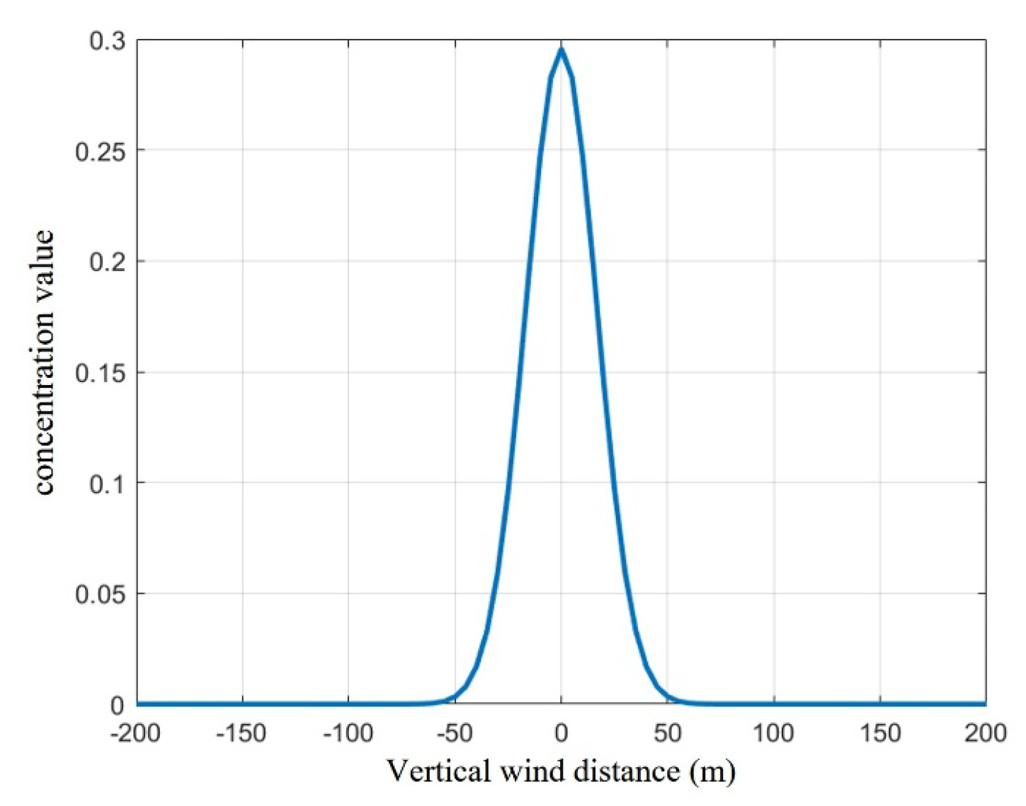
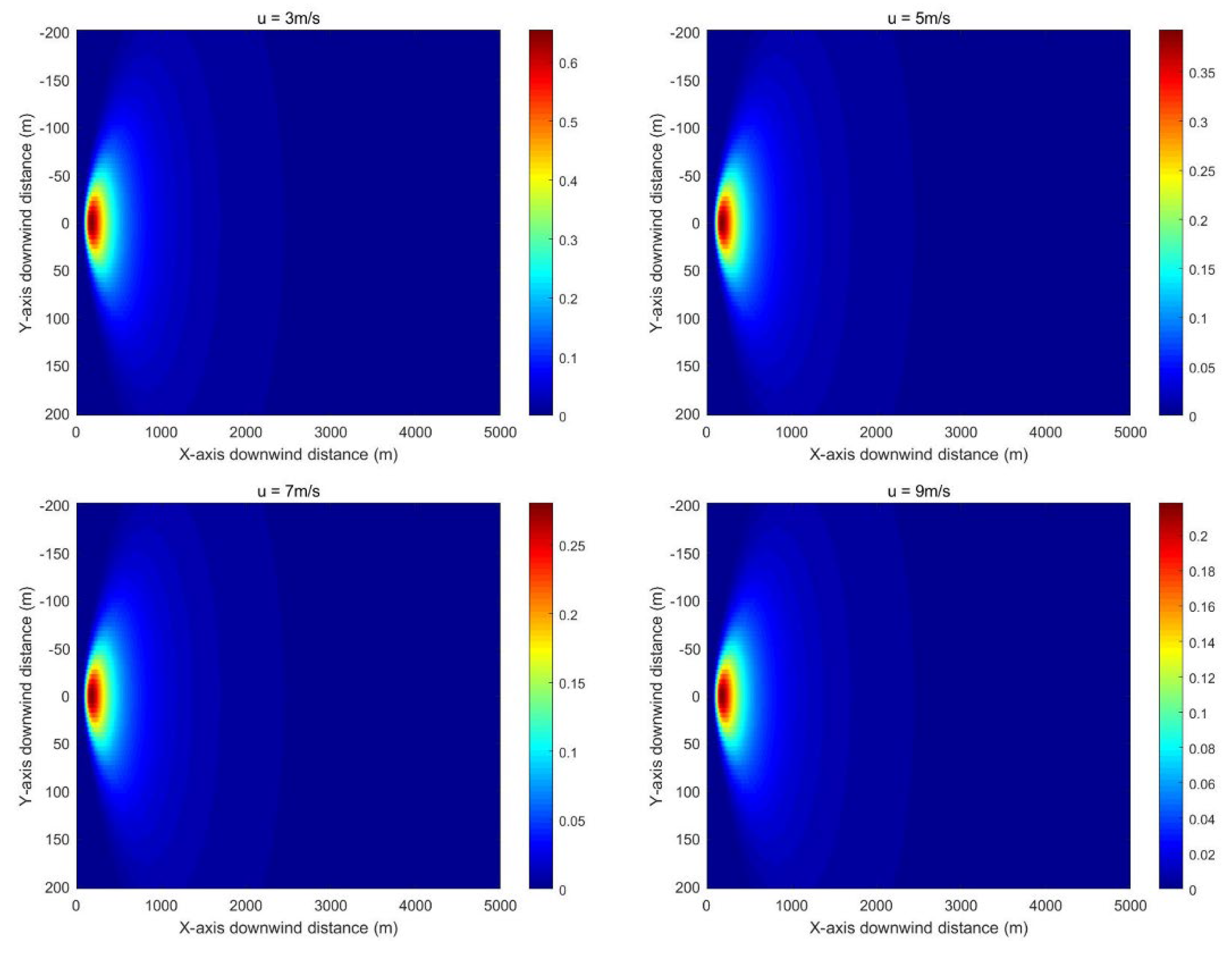
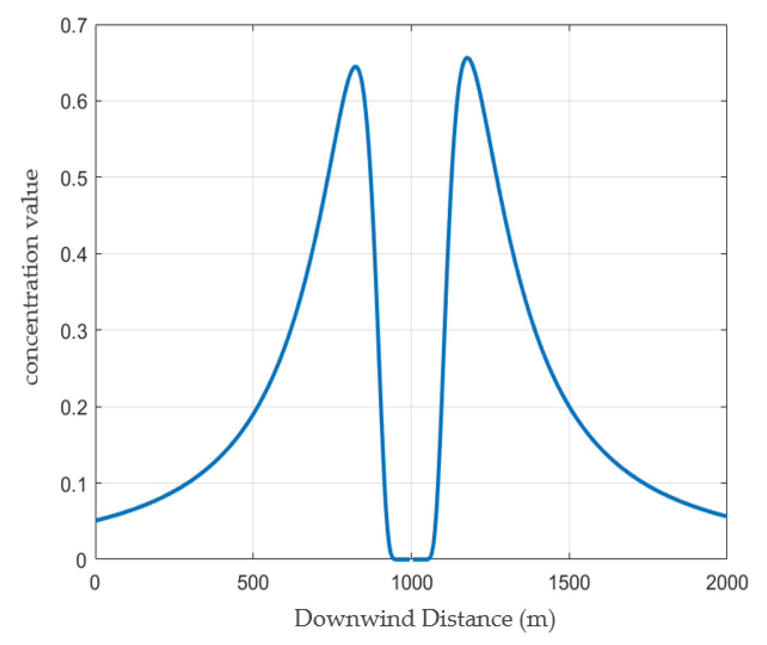
An analysis of the effects of downwind distance and vertical crosswind distance on concentration values in the Gaussian diffusion model is shown in Figure 4 and Figure 5, with carbon dioxide concentration units expressed in g/m³. As the downwind distance progressively increases, the carbon dioxide concentration initially rises sharply, subsequently decreases gradually, and ultimately approaches zero at a certain distance. This pattern fundamentally reflects the process of wind-driven dispersion and dilution following carbon dioxide emissions from the source. The vertical crosswind distance profile exhibits a normal distribution, consistent with the Gaussian diffusion model’s assumption of symmetrical normal distribution in the crosswind direction. The maximum concentration is predicted at y = 0, with progressively diminishing values towards both lateral directions.

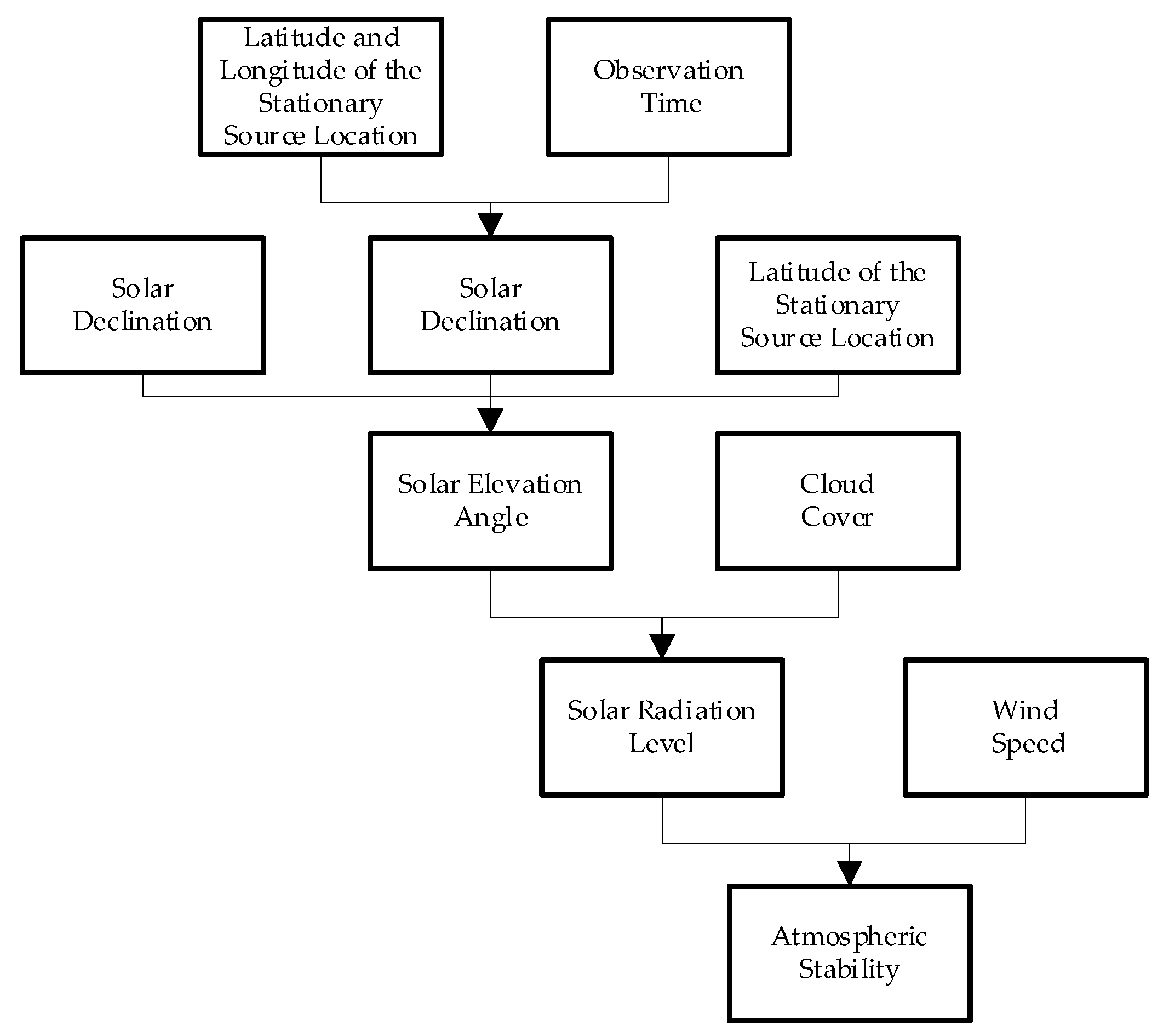
When wind speed is ≤1.5 m/s, the atmosphere approaches quasi-stagnant conditions characterized by pronounced instability. Under low-/no-wind conditions, the atmospheric dispersion of gaseous pollutants becomes significantly complex: CO₂ emissions may exhibit recirculation patterns and plume subsidence, while surface-level turbulence intensifies with heightened unpredictability. Substantial discrepancies between surface wind speed and effective stack exit velocity compromise dispersion modeling accuracy. Wind direction divergence between surface and stack exit levels, coupled with the absence of prevailing wind vectors, frequently occurs in low-wind regimes [28]. These conditions invalidate the directional axis assumption fundamental to Gaussian dispersion modeling. Consequently, the conventional Gaussian model becomes inapplicable under calm-wind scenarios. Empirical formulas are typically employed for approximation in practical applications. This approach assumes isotropic horizontal dispersion from point sources, generating concentric equi-concentration contours around emission origins. Vertical dispersion is predominantly governed by atmospheric eddy diffusivity. Turbulent transport mechanisms observed under stable wind conditions provide analogies for estimating vertical CO₂ profiles in low-wind environments. The CO₂ dispersion pattern under calm-/micro-wind conditions can be approximated by Equation (9):

$$C={({\displaystyle \frac{2}{\pi }})}^{{\displaystyle \frac{1}{2}}}{\displaystyle \frac{Q}{2\pi u{\sigma }_z}}\exp (-{\displaystyle \frac{H}{2{\sigma }_z^2}})$$

(9)

2.2. Model Revision

2.2.1. Terrain Factor Correction

The Gaussian dispersion model primarily applies to flat and open terrains, with most industrial parks situated in plain areas. Inevitably, hilly terrain exists in the southeastern sectors of industrial parks, where topographic features obstruct CO₂ dispersion from upwind emission sources. The conventional Gaussian model demonstrates limited applicability for dispersion simulations in such areas. Scholars worldwide have conducted research, with Reference [29] proposing a terrain factor to modify the Gaussian dispersion model. Reference [30] developed a complex terrain-adapted Gaussian model utilizing Digital Elevation Model (DEM) data and spatial interpolation for dispersion simulation. To address this challenge, our study incorporates terrain influences into Gaussian model modifications. For stationary CO₂ emission dispersion modeling, we introduce a terrain correction factor that integrates stack height with topographic elevation differentials.

$$C(x,y,z)={\displaystyle \frac{Q}{\pi u{\sigma }_y{\sigma }_z}}\times \exp (-{\displaystyle \frac{y^2}{2{\sigma }_y^2}})\exp (-{\displaystyle \frac{1}{2}}{\displaystyle \frac{{\left(H-h_t\right)}^2}{{\sigma }_z^2}})$$

(10)

where $H$—effective stack height of stationary source and $h_t$—terrain elevation at the specified point.

The incorporation of a terrain correction factor ensures the dynamic adjustment of the emission source effective height according to topographic undulations, thereby guaranteeing both physical rationality and modeling accuracy in simulating downwind CO₂ concentration propagation. For stationary-source CO₂ dispersion modeling, this study introduces a correction function into the Gaussian framework to enhance simulation fidelity under complex terrain conditions.

$$\begin{array}{l}C(x,y,z)=C_0\times \exp [-{\displaystyle \frac{{(x-x_0)}^2}{2{\sigma }_x^2}}-{\displaystyle \frac{{(y-y_0)}^2}{2{\sigma }_y^2}}-{\displaystyle \frac{{(z-z_0)}^2}{2{\sigma }_z^2}}\\ +{\displaystyle \frac{u(x-x_0)+v(y-y_0)+w(z-z_0)}{{\sigma }^2}}+f(x,y,z)]\end{array}$$

(11)

$$f(x,y,z)=k\times h(x,y)\times s(x,y)$$

(12)

where $h(x,y)$ is the terrain elevation function; $s(x,y)$ is the slope gradient function; and $k$ is the terrain correction coefficient.

2.2.2. Reflection Coefficient Correction

Conventionally, in Gaussian dispersion modeling under ideal impermeable and non-absorbent ground conditions, the reflection coefficient is set to unity (p = 1) for both image and real sources, indicating complete pollutant reflection into the atmosphere. However, actual industrial park surfaces with partial vegetation coverage exhibit ground absorption characteristics, resulting in reflection coefficients below unity. The modified formulation assigns p = 0.9 to account for this attenuation effect.

$$C(x,y,z,H)={\displaystyle \frac{Q}{2\pi u{\sigma }_y{\sigma }_z}}\times \exp (-{\displaystyle \frac{y^2}{2{\sigma }_y^2}})\left[\begin{array}{l}\exp (-{\displaystyle \frac{1}{2}}{\displaystyle \frac{{\left(z-H\right)}^2}{{\sigma }_z^2}})+\\ P\ast \exp (-{\displaystyle \frac{1}{2}}{\displaystyle \frac{{\left(z+H\right)}^2}{{\sigma }_z^2}})\end{array}\right]$$

(13)

2.3. Inversion of Stationary Source Strength in Industrial Parks

2.3.1. Inversion Model

In source strength calculations for stationary sources within industrial parks, emission sources are typically partitioned into basal and apical components. The basal component refers to CO₂ emission sources within stacks, such as boilers or combustion equipment. Considered as the primary emission origin, the basal source strength demonstrates higher stability and calculability [30]. This parameter can be directly derived from fuel consumption data and emission factors, yielding relatively accessible and accurate estimates. The computational methodology is formulated in Equation (11):

$$Q={\displaystyle \sum _j{P}_j}\times EF/3600$$

(14)

where $Q$ is the source strength of carbon dioxide in the industrial park (g/s); $P_j$ represents the power output of the j-th type of fuel-powered unit equipment (kW); and $EF$ denotes the emission factor for the carbon dioxide calculation (g/(kW·h)).

The top refers to the chimney mouth of stationary emission sources. Generally, the source strength at the chimney mouth may exhibit varying degrees of attenuation due to atmospheric diffusion and turbulent dispersion, whereas the source strength at the chimney base remains more stable and accurate. The top source strength can only be inversely derived through Gaussian dispersion modeling. An appropriate Gaussian dispersion model is established based on operational data from CO₂ stationary sources and collected environmental parameters, with model variables assigned known quantitative values. Air quality monitoring data around the stationary-source chimney are collected, encompassing CO₂ concentrations and relevant meteorological parameters. The model is initially validated using chimney base-derived source strength as an input, comparing predicted pollutant concentrations with field measurements. Parameter calibration is performed iteratively until satisfactory model–measurement agreement is achieved. Inverse modeling techniques are employed, utilizing ambient monitoring concentration data to inversely calibrate Gaussian model parameters for determining the effective source strength at the chimney top [31].

The inversion calculation of CO₂ emission source strength in industrial parks can be conceptualized as an optimization problem-solving process that employs computational models to identify optimal solutions [28]. This process requires the creation of an objective function designed to minimize the error between field-measured CO₂ concentrations from monitoring devices and model-calculated values derived through Gaussian dispersion modeling. This study implements the least squares method, formulating the objective function as the sum of squared errors between measured and simulated CO₂ concentrations to solve the minimization optimization problem. We let $C_{mes}^i$ denote the CO₂ concentration at the i-th monitoring position calculated by the Gaussian model, and $C_{comp}^i$ represent the corresponding measured value. The industrial park under study deploys 24 monitoring devices. The objective function is expressed in Equation (12):

$$\min f(Q)={\displaystyle \sum _{i=1}^n{(C_{mes}^i-C_{comp}^i)}^2}$$

(15)

where $\min f(Q)$ represents the error minimization of stationary-source strength in the industrial park; $C_{mes}^i$ denotes the calculated CO₂ concentration at the i-th monitoring device location (g/m³); and $C_{comp}^i$ indicates the measured CO₂ concentration obtained from the i-th monitoring device (g/m³).

The $C_{comp}^i$ can be obtained from Equation (13):

$$\min f(Q)={\displaystyle \sum _{i=1}^n\begin{array}{l}(C_{mes}^i-\frac{Q_i}{2\pi u{\sigma }_y{\sigma }_z}\times \exp (-\frac{y^2}{2{\sigma }_y^2})\\ \left[\exp (-\frac{1}{2}\frac{{\left(z-H\right)}^2}{{\sigma }_z^2})+\exp (-\frac{1}{2}\frac{{\left(z+H\right)}^2}{{\sigma }_z^2})\right]{)}^2\end{array}}$$

(16)

When the objective function reaches its minimum value, the optimal solution corresponds to the inverted source strength. Consequently, the central challenge in source strength inversion lies in optimizing the alignment between Gaussian dispersion model simulations and field-measured CO₂ concentrations from monitoring devices. Compared to conventional least squares methods prone to error accumulation, particle swarm optimization demonstrates superior capability in reducing experimental errors through iterative search strategies, exhibiting marked advantages in solving such optimization problems [32].

2.3.2. Particle Swarm Optimization

Particle swarm optimization (PSO) is a swarm intelligence-based optimization algorithm inspired by the collective behavior of bird flocks, simulating social foraging dynamics to conduct optimization searches. Each bird (particle) retains the memory of its optimal discovered position, termed the personal best position (PBest), during the search process. The algorithm also tracks the global best position (GBest) achieved collectively by the swarm. In PSO implementation, particles are initialized with velocity and position vectors. During iterative computation, these vectors are dynamically adjusted based on both the individual historical optimum PBest and the swarm’s global historical optimum GBest. The sharing of individual optima across the swarm enables the coordinated exploration of the solution space towards optimal regions. Through collaborative swarm intelligence and information-sharing mechanisms, the particle population progressively converges to the global optimum, thereby optimizing the objective function.

Given the inherent complexity of atmospheric dispersion processes and their significant dependence on meteorological conditions, employing sum of squared errors as the objective function may prove insufficient for meeting the precision requirements in emission source strength inversion analyses. The PSO algorithm exhibits exceptional versatility in effectively addressing challenges intractable to conventional optimization techniques, while enabling comprehensive exploration across diverse objective function spaces. Compared to alternative optimization algorithms, PSO demonstrates a notable implementation simplicity by eliminating genetic operators (crossover/mutation) from genetic algorithms and pheromone update mechanisms from ant colony optimization. Featuring accelerated convergence rates, PSO maintains individual particle historical optimization data that enhance the solution space exploration efficiency while improving algorithmic robustness. The PSO framework fundamentally comprises particle entities, swarm populations, fitness evaluation metrics, and personal best PBest and GBest solutions as core operational components [22].

In PSO-based source strength inversion, each particle embodies a potential solution for CO₂ emission source strength estimation, while the swarm collectively engages in an optimization search process through coordinated particle interactions. Each particle dynamically updates its positional coordinates through social learning from swarm experiences, progressively refining CO₂ source strength solutions towards optimality. The fitness function in source inversion quantifies the discrepancy between field observations and model predictions, where minimized fitness values correspond to optimized source strength solutions [33]. During PSO iterations, particles update their velocity vectors and positional states based on PBest and GBest solutions, thereby evolving their represented source strength parameters. This evolutionary process iterates until predefined termination criteria (e.g., convergence thresholds) are satisfied, driving the swarm towards global optimum source strength determination. The fundamental workflow for PSO-driven source strength inversion is systematically illustrated in Figure 6.

As depicted in the figure, the workflow for PSO-based source strength inversion proceeds through the following stages [21,34]:

(1)

Source Strength Initialization

The initial source strength is set to 10,000 g/s with swarm size = 100 particles, maximum iterations = 100 generations, and search range = 5000–20,000 g/s. The inertia weight (w) is initialized at 0.5. Random particle positions and velocities are generated via the rand function, followed by fitness evaluations for each source strength candidate.

(2)

Personal and Global Best Solutions

Each particle’s fitness is evaluated to determine its PBest. The GBest is identified through swarm-wide comparisons.

(3)

Velocity and Position Update

Particle velocity vectors and positional states are updated iteratively. Newly generated solutions undergo fitness re-evaluation to update PBest/GBest records. The update mechanism follows Equations (14) and (15), with the particle swarm parameters (cognitive coefficient $c_1$ and social coefficient $c_2$) both set to 2.

$$v_i(n+1)=w{v}_i(n)+c_1{r}_1[P_i-x_i(n)]+c_2{r}_2[P_g-x_i(n)]$$

(17)

$$x_i(n+1)=x_i(n)+v_i(n+1)$$

(18)

(4)

Optimal Solution Output

The iterative process terminates upon reaching 100 generations, yielding the optimized source strength solution as the final output.

2.4. Methodological Flow

This study initially modified the Gaussian plume model for complex terrain conditions. It subsequently employed the modified model to perform inverse emission rate calculations, and ultimately established a regional multi-source Gaussian plume model based on heterogeneous emission sources within the industrial park. The specific workflow process is illustrated in Figure 7.

3. Results and Discussion

3.1. Source Strength Inversion Results

Industrial parks typically contain multiple stationary CO₂ emission sources distributed across extensive areas. Despite the spatial separation between sources, overlapping emission plumes may lead to compromised accuracy in source strength inversion. The Gaussian dispersion model developed in this study may encounter interference effects during source strength inversion in such multi-source environments. Each source strength inversion process is subject to superimposed impacts from adjacent emitters, as atmospheric monitoring data inherently reflect aggregated CO₂ concentrations from multiple concurrent sources under the model’s multi-source interaction framework. Consequently, emission sources exhibit interdependent superposition rather than operating independently during concurrent operations [32].

This study addresses this challenge by developing a CO₂ dispersion modeling framework that ensures independence and non-correlation between emission sources during source strength inversion. Temporal segregation is achieved through the operational scheduling of stationary sources, decoupling emission activities across distinct time windows to mitigate cross-source interference and reduce emission correlation coefficients. Concurrent process flow optimization implements granular adjustments to production sequences and operational planning, effectively flattening emission peaks through temporal load balancing to prevent the overlapping of high-intensity discharges.

For a designated stationary emission source (longitude 105.754) in an industrial park, the baseline CO₂ emission rate of 10,000 g/s derived from base source strength calculations serves as initial input to validate the PSO-based inversion accuracy for Gaussian dispersion model parameterization. Multiple CO₂ monitoring devices deployed concentrically around the emission source provide spatiotemporal measurement data (

Table 3. Partial monitoring device data.

Monitoring Device ID	Concentration Data (g/m3)	Local Coordinates (m)
1	0.642864	(170, 5)
2	0.572373	(225, −10)
3	0.376471	(305, −25)
4	0.496802	(170, −20)
5	0.466632	(125 −5)
6	0.353232	(205, −35)
7	0.135505	(570, −50)
8	0.212652	(360, −55)
9	0.281891	(245 −45)
10	0.466632	(125, −5)

) essential for model inversion computations.

To validate the feasibility of PSO for stationary-source strength inversion, this study conducts iterative problem-solving under open-terrain conditions in an industrial park. The simulation setup initializes a CO₂ emission source at 10,000 g/s, with specified meteorological parameters: wind speed = 3 m/s and Atmospheric Stability Class B. The Gaussian dispersion model is parameterized with cognitive coefficient $c_1$ = 2, social coefficient $c_2$ = 2, swarm size = 100 particles, maximum iterations = 100 generations, inertia weight bounds [0.4, 0.9], and source strength search domain = 5000–20,000 g/s. Velocity initialization employs inertia weight w = 0.5.

As demonstrated in Figure 8, the PSO-driven optimization process minimizes source strength errors using tabular data. After stable iterative computations, the algorithm converges to an inverted CO₂ emission rate Q = 9986.4986 g/s (longitude 105.76464, latitude 32.40131), yielding an absolute error of 13.5014 g/s (0.135% relative error) compared to the initial source strength. The inverted source strength exhibits rapid convergence during initial iterations, achieving stabilization at the 24th generation, with full computational completion at 100 iterations. This implementation demonstrates PSO’s computational efficacy in source inversion, characterized by accelerated convergence, sub-second computational latency, and laboratory-grade precision, establishing high referential value for industrial applications.

Figure 9 illustrates the co-evolution of optimal source strength values (Q) and their corresponding fitness (F) across iterations. The fitness metric exhibits a steep descent during the initial 10 generations, reaching F = 8.7389 × 10⁻⁷ at the 10th iteration, demonstrating remarkable optimization progress. Stabilization initiates around the 24th iteration (F = 7.3509 × 10⁻⁷) as the swarm progressively approaches the global optimum. The algorithm successfully converges to the globally optimized source strength after completing 100 predefined iterations.

The application of the PSO algorithm for fixed-source emission rate inversion not only ensures rapid convergence and a shorter iteration time, but also guarantees high-precision computational results. For both carbon dioxide and other hazardous gases, the high-efficiency computation in industrial park fixed-source intensity inversion can significantly reduce the data processing time and enhance the emergency response speed. Particularly in industrial park environmental accidents, obtaining leakage source intensity values quickly and accurately facilitates enterprises in formulating effective response measures. Therefore, the inversion of fixed-source emission intensity using the particle swarm optimization algorithm demonstrates substantial application prospects.

3.2. Simulation of Stationary Single-Point Source CO₂ Dispersion Model

The main factors affecting the accuracy of concentration–dispersion models are the atmospheric dispersion system and atmospheric stability, and these two main factors are described in this section.

3.2.1. Influencing Factor

The atmospheric diffusion coefficient is an important parameter that describes the diffusion ability of pollutants in the atmosphere, and is one of the important parameters affecting Gaussian diffusion modeling [29]. The lateral diffusion coefficient ${\sigma }_y$ describes the diffusion of pollutants perpendicular to the plane of wind direction, and the vertical diffusion coefficient ${\sigma }_{\mathrm{z}}$ describes the spatial diffusion ability of pollutants perpendicular to the ground upwards, with the following formula:

$$\begin{array}{l}{\sigma }_y=r_1{x}^{{\alpha }_1}\\ {\sigma }_{\mathrm{z}}=r_2{x}^{{\alpha }_2}\end{array}$$

(19)

where $r_1$ and ${\alpha }_1$ are the coefficients and indices for calculating the lateral diffusion parameters; and $r_2$ and ${\alpha }_2$ are the coefficients and indices for calculating the vertical diffusion parameters. These coefficients can be obtained from

Table 4. Expressions for transverse parameters.

Atmospheric Stability	${\mathit{\alpha }}_1$	${\mathit{r}}_1$	Leeward Distance
A	0.901074	0.425809	0–1000
	0.850934	0.602052	>1000
B	0.914370	0.281846	0–1000
	0.865014	0.396353	>1000
C	0.924279	0.177154	0–1000
	0.885157	0.232123	>1000
D	0.929418	0.110726	0–1000
	0.888723	0.146669	>1000
E	0.920818	0.0864001	0–1000

and

Table 5. Vertical parameter expressions.

Atmospheric Stability	${\mathit{\alpha }}_2$	${\mathit{r}}_2$	Leeward Distance
A	1.12154	0.07999	0–300
	1.51360	0.00854	300–500
B	2.10881	0.00021	>500
	0.964435	0.127190	0–500
C	1.09356	0.057025	>500
	0.917595	0.106803	>0
D	0.826212	0.104634	1–1000
	0.632023	0.400167	1000–10,000
E	0.788370	0.092752	0–1000
	0.565188	0.533384	1000–10,000
F	0.784400	0.062076	0–1000
	0.525969	0.370015	1000–10,000

.

Atmospheric stability refers to the ability of the atmosphere to inhibit or promote vertical motion, which is a parameter reflecting the state of atmospheric turbulence and has a significant impact on the diffusion process of gases such as carbon dioxide. In this paper, the atmospheric stability is determined based on the Pasquill stability classification method, and the process is shown in Figure 10.

The Pasquill method divides atmospheric stability into six classes: A (strongly unstable), B (unstable), C (weakly unstable), D (neutral), E (weakly stable), and F (stable). Some of the data are shown in

Table 6. Definition of atmospheric stability.

Ground Wind Speed (m/s)	Solar Radiation Level
	+3	+2	+1	0	−1	−2
≤1.9	A	A–B	B	D	E	F
2–2.9	A–B	B	C	D	E	F
3–4.9	B	B–C	C	D	D	E
5–5.9	C	C–D	D	D	D	D
≥6	D	D	D	D	D	D

[22] (refer to GB3840-83).

Simulations of the diffusion model of carbon dioxide concentration emitted from stationary sources were carried out through MATLAB to analyze the diffusion characteristics and the influencing factors by considering the diffusion of different wind speeds, atmospheric stabilities, and altitudes. Based on the actual situation of a thermal power plant, such as its fuel type and combustion efficiency, the simulation parameters are set as shown in

Table 7. Parameters of stationary-source simulations.

Parameters	Source Strength	Initial Wind Speed	Effective Source Height of Emission Sources	Reflectance	Step Size	Topographic Corrections
notation	Q	$u$	$H$	$P$	s	F
unit (of measure)	g/s	m/s	m	/	m	/
value	9986.4986	3	30	0.9	5	0

.

3.2.2. Atmospheric Stability Comparison

Based on six atmospheric stability levels (A, B, C, D, E, F), the diffusion of carbon dioxide from a stationary source in a thermal power plant is simulated under constant conditions such as wind speed, and the diffusion of carbon dioxide concentration on the ground at z = 0 is plotted to discuss the diffusion pattern of the carbon dioxide concentration under different atmospheric stability levels.

As shown in Figure 11, with the change in Atmospheric Stability Class, the CO₂ convection is relatively weakened, the stable atmospheric conditions significantly limit the vertical diffusion, and the diffusion rate of CO₂ concentration is relatively slow. At the same time, the highest concentration value is becoming smaller and smaller from about 0.79 g/s in Atmospheric Stability Class A to about 0.3 g/s in Atmospheric Stability Class F. Under more stable atmospheric conditions, the air layer becomes more laminar, leading to a tendency for the concentration of carbon dioxide in the air layer to decrease. Because the air layer is smoother under the more stable atmospheric conditions, the vertical diffusion is limited, so the horizontal diffusion of carbon dioxide in the ground layer moves in the downwind direction, and the propagation distance in the downwind direction gradually increases, resulting in the concentration area of the highest concentration being farther and farther away, and the concentration being gradually reduced.

3.2.3. Wind Speed Comparison

Comparative experiments on wind speed were conducted by keeping the atmospheric stability at a constant Class B, setting the initial wind speed at 3 m/s, and adding three sets of data, 5 m/s, 7 m/s, and 9 m/s, to discuss the diffusion pattern of the carbon dioxide concentration under different wind speeds.

As shown in Figure 12, unlike the atmospheric stability comparison test, the change in wind speed did not affect the location of the highest concentration point downwind. When the wind speed was 3 m/s, the highest concentration in the high concentration area was 0.67 mg/m³; as the wind speed increased to 5 m/s, the highest concentration in the high concentration area decreased to 0.39 mg/m³; when the wind speed continued to increase to 7 m/s, the highest concentration in the high concentration area further decreased to 0.28 mg/m³; and when the wind speed was 9 m/s, the highest concentration in the high concentration area was 0.21 mg/m³. The maximum concentration was 0.21 mg/m³. Under higher wind speed conditions, carbon dioxide was more readily diluted and rapidly dispersed, resulting in a decrease in the peak air concentration of carbon dioxide as wind speed increased.

3.2.4. Effective Height Comparison

Comparative experiments were conducted on effective heights, and four different groups of effective heights were set up, namely 30 m, 50 m, 60 m, and 70 m, with no change in other conditions, to analyze the effect of effective heights on the diffusion of carbon dioxide.

As shown in Figure 13, the greater the effective height, the larger the diffusion area of carbon dioxide. The highest concentration value of carbon dioxide gradually decreased; when the height of the emission source was 30 m, the highest concentration was 0.65 g/m³; when it rose to 50 m, the highest concentration decreased to 0.23 g/m³; when it rose to 60 m, the highest concentration decreased to 0.15 g/m³; and finally, when it rose to 70 m, the maximum concentration decreased to 0.12 g/m³, and the rate of decrease gradually slowed down. The higher the effective height, the greater the carbon dioxide diffusion area, the lower the concentration at the highest point, and the wider the influence range of carbon dioxide. This is because an increase in the height of the emission source elevates the starting point of the diffusion process, thereby relatively increasing the vertical diffusion space for carbon dioxide. This may lead to a reduction in the concentration of carbon dioxide received at ground level.

By simulating the effect of three different parameters on the CO₂ diffusion model, it was found that the model with correction for the reflection coefficient and topography was better than the other models. It was more stable under the three influencing parameters.

(1) Under stable conditions (Class F), suppressed vertical turbulence restricted CO₂ dispersion predominantly to the horizontal plane, resulting in a 30% increase in near-ground concentration peaks compared to unstable conditions (Class C). In contrast, strong convection in unstable conditions (Class B) induced rapid CO₂ elevation, generating concentrations twice as high as stable conditions at a 200 m altitude, while reducing near-ground concentrations by 40%. (2) At wind speeds >6 m/s, terrain-induced flow separation caused plume bifurcation, creating dual concentration peak zones with horizontal displacement reaching 300 m. When wind speeds dropped below 3 m/s, CO₂ accumulated near the source with steep concentration gradients, where the model-predicted 1 h average concentrations showed strong agreement with ground sensor data. (3) The maximum near-ground (10 m) concentration decreased by 28%, whereas concentrations at a 200 m altitude increased by 15%, indicating that merely increasing stack height may exacerbate elevated pollution. This finding demonstrates a fundamental consistency with the variation patterns of atmospheric pollutants predicted by Gaussian models in reference studies.

3.3. Simulation of CO₂ Dispersion Model for Stationary Multi-Point Sources

Conventional CO₂ dispersion models for stationary sources assume coordinate systems with the emission source at the origin (X = 0). However, when modeling multiple stationary sources within a wind-aligned coordinate system (X-axis downwind), individual sources require distinct spatial coordinates. Each emission source occupies unique (X, Y) coordinates, serving as initial release points for dispersion calculations. In this industrial park case study, ten stationary sources exhibit heterogeneous emission characteristics (varying source strengths) and require individualized geospatial parametrization.

The codebase is upgraded to implement a generalized single-source CO₂ dispersion model, where the emission source is localized at (1000, 100) in Cartesian coordinates rather than the default origin (0, 0). Figure 14 illustrates the dispersion pattern originating from the stationary source at (1000, 100), demonstrating omnidirectional propagation characteristics. Contrary to unidirectional advection assumptions, the simulation reveals radially symmetric dispersion governed by turbulent mixing mechanisms. Lateral dispersion develops perpendicular to the mean wind direction due to atmospheric turbulence effects quantified by the eddy diffusivity tensor. The concentration field exhibits mirror symmetry about the x = 1000 plane, with identical iso-concentration contours in both the windward and leeward directions.

As shown in Figure 15, the concentration distribution profile along the downwind X-axis at y = 100 is presented. For both sides of the 1000 m position, the concentration values first increase to a specific peak value, then gradually decrease and approach zero. Figure 15 more clearly demonstrates the symmetry of carbon dioxide diffusion, where the diffusion rates at both lateral boundaries are essentially identical, and the concentration at the 1000 m point remains zero. This phenomenon is primarily determined by the mathematical properties inherent in the Gaussian diffusion model. Under the assumptions of uniform wind speed and stable atmospheric conditions, pollutant dispersion downwind will exhibit symmetry, particularly along the direct line from the source at x = 1000. Since the Gaussian diffusion model is based on the normal distribution principle, the concentration variation along the X-direction conforms to a normal distribution, resulting in this symmetric distribution pattern.

Comparative data analysis reveals that the maximum concentration on the left side reaches 0.644 g/m³, while the right side attains a peak value of 0.656 g/m³. The downwind distance corresponding to the peak concentration measures 820 m on the left side and approximately 1175 m on the right side. The left peak position deviates 180 m from the theoretical symmetry point, whereas the right side shows a 175 m deviation. In simulation experiments, the minor discrepancies may arise from discretization or iterative errors introduced during the numerical solution of the model’s differential equations. In practical engineering scenarios, carbon dioxide dispersion may demonstrate asymmetry due to complex factors including wind speed/direction variability, surface roughness, thermal gradients, and topographic effects. However, the idealized Gaussian diffusion model conventionally assumes that these parameters remain constant.

For the 10 stationary carbon dioxide emission sources in this industrial park, simulation experiments are required in MATLAB. Meteorological conditions including wind speed and atmospheric stability are assumed to remain consistent throughout the industrial park. The particle swarm optimization algorithm is employed to solve the source strength inversion model, determining the peak emission rates for the 10 stationary sources. Stack height parameters for each emission source are provided in

Table 8. Parameters of stationary sources in industrial park.

Stationary Source ID	Geographic Coordinates	Local Coordinates	Emission Rate (g/s)	Stack Height (m)
1	(105.754, 32.404)	(0, 0)	11,591.547	70
2	(105.76464, 32.40131)	(1000, −300)	9986.4986	30
3	(105.76464, 32.404)	(1000, 0)	7978.4231	50
4	(105.76996, 32.40041)	(1500, −400)	6498.2	50
5	(105.76996, 32.39861)	(2000, −480)	6543.3	50
6	(105.77528, 32.39969)	(1500, −600)	3569.224	40
7	(105.7806, 32.404)	(2500, 0)	3250.42	30
8	(105.78411, 32.40041)	(2830, −400)	6520.49	50
9	(105.78592, 32.39771)	(3000, −700)	5920.4	50
10	(105.78486, 32.39592)	(2900, −900)	6021.23	50

.

The atmospheric stability is determined to be Class B based on the collected meteorological conditions, with wind speed and direction assumed to remain steady at a magnitude of 2 m/s. Simulation experiments are conducted on the multi-source CO₂ dispersion model for stationary sources using tabular data, investigating the dispersion characteristics under multiple emission source conditions. Figure 16 illustrates the 2D and 3D dispersion patterns of the multi-source Gaussian plume model for stationary sources. The morphological distribution of multi-source Gaussian dispersion demonstrates irregular patterns, predominantly concentrated along the negative y-axis direction. This phenomenon stems from coordinate transformation analysis revealing that stationary sources are primarily located in the negative y-axis orientation within the local coordinate system.

Simulation results indicate dual peak concentration values at coordinates (1185, −305) and (835, −300), both approximating 0.72 g/m³, consistent with the symmetry of the Gaussian dispersion model’s normal distribution. The peak concentration is predominantly attributed to the emission source at (1000, −300) with elevated emission rate parameters. Compared to single-source dispersion modeling, the peak concentration increases significantly from 0.65 g/m³ due to superposition effects from adjacent emission sources. The emission source at (1000, 0) with a 7978.4231 g/s emission rate generates the maximum concentration of 0.24 g/m³ at coordinate (1300, 0). Superposition with the origin source (11,591.547 g/s) results in an asymmetric maximum concentration of 0.29 g/m³, demonstrating source interaction effects. The remaining emission sources maintain normal distribution symmetry, except the aforementioned coordinates. The simulation reaffirms the inverse relationship between effective stack height and peak concentration, with dispersion range expansion conforming to previous height comparison simulations. The influences of atmospheric stability and wind speed on CO₂ dispersion patterns similarly adhere to their respective foregoing conclusions.

4. Conclusions

This study developed a concentration dispersion model tailored for fixed-source CO₂ emissions in industrial park complexes. Initially, a Gaussian-based dispersion model was constructed for stationary CO₂ emission sources, subsequently modified with corrections, accounting for image source effects and plume rise height. A representative fixed emission source was selected for parametric simulation, with operational parameters configured according to typical industrial scenarios. Three comparative experiments (atmospheric stability, wind speed, and effective height variations) were conducted to analyze the dispersion characteristics of fixed-source CO₂ emissions. The ultimate findings demonstrated that these three parameters constitute primary determinants of fixed-source CO₂ dispersion patterns. Enhanced atmospheric stability correlated with reduced dispersion velocity, causing the high-concentration zone to extend farther from the source. While wind speed variations preserved dispersion geometry, higher velocities accelerated dilution processes, resulting in an 18–22% peak concentration reduction per 1 m/s increment. The higher the emission source elevation, the lower the peak CO₂ concentration levels observed. Finally, to address the differential attenuation of source strength at the bottom and top layers, a fixed-source inverse calculation model was developed, incorporating the PSO algorithm for solution derivation. The optimization achieved superior fitness levels, with the results demonstrating minimum error rates, fewer iterations, shorter computation times, and a high applicability in practical scenarios. Compared to conventional on-site monitoring approaches, the numerical modeling framework achieved high-precision spatial concentration reconstruction using limited discrete sampling points. This methodology substantially reduced both the economic and temporal costs associated with pollutant concentration field mapping. The approach provided an operational technical pathway for regional environmental quality assessment.

This study has three main limitations: First, the model validation framework is currently confined to the emission characteristics of stationary point sources like coal-fired power plants (CFPPs), failing to adequately address the differentiated validation needs for urban traffic sources (with distinct pulsed emission characteristics) and process industrial sources such as steel metallurgy (exhibiting intermittent high-intensity emission patterns). Second, regarding adaptability to dynamic emission scenarios, the simulation accuracy of existing models for transient emission responses caused by vehicle acceleration/idling operating conditions in transportation networks has not been systematically validated. Third, in meteorological parameter processing, the current model adopts a constant humidity assumption without the adequate incorporation of precipitation phase-change processes and dew-point temperature fluctuations that potentially affect boundary layer stability and pollutant dispersion pathways.

Future research should advance model optimization through four dimensions: (1) Multi-source emission system expansion: Establishing a multi-scale validation framework encompassing offshore oil/gas platforms (with air–sea interface evaporation effects) and urban industrial complexes (coupled with urban heat island circulation impacts), focusing on analyzing the interaction mechanisms between building cluster flow fields and CO₂ dispersion. (2) Complex environmental coupling modeling: Integrating multi-parameter real-time data streams from Weather Research and Forecasting meteorological models to develop a data assimilation-based dynamic CO₂ concentration field forecasting system, achieving hourly resolution predictions of atmospheric dispersion processes. (3) Computational fluid dynamics acceleration: Implementing a CNN-LSTM hybrid architecture for the surrogate modeling of conventional RANS turbulence models, reducing the simulation time for typical scenarios to sub-hour levels through transfer learning strategies. (4) Dynamic environmental factor coupling: Developing a meteorological element feedback-corrected dynamic humidity module to quantitatively assess the spatial redistribution effects of precipitation scavenging on near-surface CO₂ concentration distributions. Notably, implementing these technical pathways requires establishing cross-scale observational validation networks, particularly high-resolution flux monitoring systems for specialized environments like offshore platforms and urban canopies.

References

1. Wu, X.; Zhu, F.; Yang, J.; Zhou, D.; Yan, L.; Teng, N.; Yi, Y. Measurement of greenhouse gas emission factors in thermal power generation industry. Environ. Sci. Res. 2010, 23, 170–176. [Google Scholar]
2. Zhou, Y.; Cai, B.; Liu, L.; Cao, D. Study on the spatial distribution of carbon dioxide emissions in China’s thermal power industry. Therm. Power Gener. 2011, 40, 1–3+7. [Google Scholar]
3. Ma, X.; Wang, X.; Sun, X.; Shi, J.; Chen, J.; Dang, L. Study on the influencing factors of carbon emission intensity of coal-fired power generation units. Therm. Power Gener. 2022, 51, 190–195. [Google Scholar] [CrossRef]
4. Sun, Y.; Zheng, Z.; Qin, Y.; Guo, Z.; Ren, J. Research on carbon emission characteristics of thermal power units and management suggestions. China Electr. Power 2018, 51, 144–149. [Google Scholar]
5. Jiang, W. Tutorial on Air Pollution Meteorology; Meteorological Press: Beijing, China, 2004; p. 285. [Google Scholar]
6. Seibert, P. Iverse modelling with a lagrangian particle dispersion model: Application to point releases over limited time intervals. In Air Pollution Modeling and Its Application XIV; Springer: Boston, MA, USA, 2004; pp. 381–389. [Google Scholar]
7. Ma, H.; Xing, Z.; Wu, F.; Wu, J. Research on prediction accuracy of Gaussian diffusion model based on orthogonal test method. China Saf. Prod. Sci. Technol. 2023, 19, 164–170. [Google Scholar]
8. Shi, B.; Nie, S.; Sun, J. Investigation on LPG leakage anddiffusion based on Gaussian plumemixture model. J. Saf. Environ. 2022, 22, 909–918. [Google Scholar]
9. Wang, H.D.; Mo, Z.X. Simulation analysis of liquid ammonia storage tank leakage diffusion based on Gaussian model. Chin. J. Saf. Sci. 2012, 22, 31–36. [Google Scholar]
10. Zheng, H.; Wu, B.; Xu, F.; Zhang, M.; Qi, X. Visualization of Soild Waste Incineration Exhaust Emissions Based on Gaussian Diffusion Model. Comput. Sci. 2019, 46, 527–531. [Google Scholar]
11. Chen, J. Dispersion Simulation Study of Pollutants from Ships in Xiamen Harbor Based on Web GIS and Gaussian Atmospheric Modeling. Master’s Thesis, Xiamen University, Xiamen, China, 2017. [Google Scholar]
12. Lu, S.; Zhang, Y.; Wu, W.; Yang, F.; Liu, L.; Kang, G.; Li, Q.; Cheng, H.; Wang, N.; Wang, F.; et al. Health risk assessment of nitrosamine diffusion from a megaton CO2 capture project. Chem. Prog. 2023, 42, 3209–3216. [Google Scholar]
13. Zhang, Q.; Guo, R.; Zhang, C.; Chen, X.; Wang, B. Radioactive airborne effluents and the environmental impact assessment of CAP1400 nuclear power plant under normal operation. Nucl. Eng. Des. 2014, 280, 579–585. [Google Scholar] [CrossRef]
14. Pournazeri, S.; Princevac, M.; Venkatram, A. Scaling of building affected plume rise and dispersion in water channels and wind tunnels—Revisit of an old problem. J. Wind. Eng. Ind. Aerodyn. 2012, 103, 16–30. [Google Scholar] [CrossRef]
15. Chen, D.; Nie, B.; Ran, Y.; Wang, Y.; Li, H.; Gu, W.; Wang, D. Improved Gaussian plume model for atmospheric dispersion considering buoyancy and gravitational deposition: The case of multi-form tritium. Appl. Radiat. Isot. 2023, 199, 110892. [Google Scholar] [CrossRef]
16. Chen, S.; Broday, D.M. Re-framing the Gaussian dispersion model as a nonlinear regression scheme for retrospective air quality assessment at a high spatial and temporal resolution. Environ. Model. Softw. 2020, 125, 104620. [Google Scholar] [CrossRef]
17. Cheng, S. Practical Methods and Techniques for Monitoring Emissions from Stationary Sources; China Environmental Science Press: Beijing, China, 1997. [Google Scholar]
18. Li, Y.Y. Improvement of Gaussian Smoke Plume Model and Its Application in the Simulation of Hazardous Chemical Leakage Accident. Ph.D. Thesis, Guangzhou University, Guangzhou, China, 2013. [Google Scholar]
19. Fu, J.Y.; Li, Y. Study on ship’s exhaust-gas diffusion based on Gaussian plume model. Mar. Sci. Bull. 2018, 37, 235–240. [Google Scholar]
20. He, H.; Peng, Y.; Ling, M. Discussion on the impact of terrain undulation on gas diffusion based on the Gaussian model. Geospat. Inf. 2015, 13, 3. [Google Scholar] [CrossRef]
21. Liang, J.; Kong, W.; Fei, W.; Xin, Q. Improvement of the Gaussian plume model based on complex terrain. J. Environ. Eng. 2016, 10, 5. [Google Scholar]
22. Shi, T.; Han, G.; Ma, X.; Zhang, M.; Pei, Z.; Xu, H.; Qiu, R.; Zhang, H.; Gong, W. An inversion method for estimating strong point carbon dioxide emissions using a differential absorption Lidar. J. Clean. Prod. 2020, 271, 122434. [Google Scholar] [CrossRef]
23. U.S. Environmental Protection Agency. Clean Air Act Standards and Guidelines for Petroleum Refineries and Distribution Industry. Available online: https://www.epa.gov/stationary-sources-air-pollution/clean-air-act-standards-and-guidelines-petroleum-refineries-and (accessed on 6 June 2019).
24. Humphries, R.; Jenkins, C.; Leuning, R.; Zegelin, S.; Griffith, D.; Caldow, C.; Berko, H.; Feitz, A. Atmospheric tomography: A Bayesian inversion technique for determining the rate and location of fugitive emissions. Environ. Sci. Technol. 2012, 46, 1739–1746. [Google Scholar] [CrossRef]
25. Kuske, T.; Jenkins, C.; Zegelin, S.; Mollah, M.; Feitz, A. Atmospheric tomography as a tool for quantification of CO2 emissions from potential surface leaks: Signal processing workflow for a low accuracy senor array. Energy Procedia 2013, 37, 4065–4076. [Google Scholar] [CrossRef]
26. Feitz, A.; Jenkins, C.; Schacht, U.; McGrath, A.; Berko, H.; Schroder, I.; Noble, R.; Kuske, T.; George, S.; Heath, C.; et al. An assessment of near surface CO2 leakage detection techniques under Australian conditions. Energy Procedia 2014, 63, 3891–3906. [Google Scholar] [CrossRef]
27. Jenkins, C.; Kuske, T.; Zegelin, S. Simple and effective atmospheric monitoring for CO2 leakage. Int. J. Greenh. Gas Control 2016, 46, 158–174. [Google Scholar] [CrossRef]
28. Di Gilio, A.; Palmisani, J.; Petraccone, S.; de Gennaro, G. A sensing network involving citizens for high spatio-temporal resolution monitoring of fugitive emissions from a petroleum pre-treatment plant. Sci. Total Environ. 2021, 791, 148135. [Google Scholar] [CrossRef]
29. Zheng, B.; Chevallier, F.; Ciais, P.; Broquet, G.; Wang, Y.; Lian, J.; Zhao, Y. Observing carbon dioxide emissions over China’s cities and industrial areas with the Orbiting Carbon Observatory-2. Atmos. Chem. Phys. 2020, 20, 8501–8510. [Google Scholar] [CrossRef]
30. Ye, X.; Lauvaux, T.; Kort, E.A.; Oda, T.; Feng, S.; Lin, J.C.; Wu, D. Constraining fossil fuel emissions from urban area using OCO-2 observations of total column. J. Geophys. Res. 2020, 125, e2019JD030528. [Google Scholar] [CrossRef]
31. Mackie, K.R.; Cooper, C.D. Landfill gas emission prediction using voronoi diagrams. Environ. Model. Softw. 2009, 24, 1223–1232. [Google Scholar] [CrossRef]
32. Wang, Y.; Song, L.; Zeng, L.; Rahmat-Samii, Y. Novel hybrid particle swarm and Brainstorm optimization: Electromagnetic applications with endanced performance. IEEE Antennas Propag. Mag. 2024, 67, 19–33. [Google Scholar] [CrossRef]
33. Gao, T.; Xu, D.; Mi, Y.; Lu, Y. Simulation analysis of NO2 pollution diffusion law based on gauss plume model: A case study from Hebei province. IOP Conf. Ser. Earth Environ. Sci. 2020, 555, 012090. [Google Scholar] [CrossRef]
34. Zhang, B.C.; Zhao, J. Gaussian plume modeling for atmospheric pollution dispersion with GIS integration. Environ. Monit. Manag. Technol. 2008, 17–19, 55. [Google Scholar]
Figure 1. Schematic diagram of stationary-source emissions.
Energies 18 02827 g001
Figure 2. Ground reflection map of stationary-source emissions.
Energies 18 02827 g002
Figure 3. Schematic diagram of Gaussian diffusion model simulation: (a) three-dimensional; (b) two-dimensional.
Energies 18 02827 g003
Figure 4. Effect of downwind distance on concentration.
Energies 18 02827 g004
Figure 5. Effect of vertical crosswind distance on concentration.
Energies 18 02827 g005
Figure 6. Flowchart of particle swarm algorithm to back-calculate source strength.
Energies 18 02827 g006
Figure 7. Workflow diagram.
Energies 18 02827 g007
Figure 8. Variation in source strength Q with iteration count.
Energies 18 02827 g008
Figure 9. Variation in fitness F with iteration count.
Energies 18 02827 g009
Figure 10. Flowchart for calculating atmospheric stability.
Energies 18 02827 g010
Figure 11. Plot of comparative simulations of atmospheric stability. (A) Atmospheric Stability Classification: Class A; (B) Atmospheric Stability Classification: Class B; (C) Atmospheric Stability Classification: Class C; (D) Atmospheric Stability Classification: Class D; (E) Atmospheric Stability Classification: Class E; (F) Atmospheric Stability Classification: Class F.
Energies 18 02827 g011
Figure 12. Graph of wind speed comparative experiment.
Energies 18 02827 g012
Figure 13. Effective height control experiment diagram.
Energies 18 02827 g013
Figure 14. Spatial distribution map of CO2 dispersion at arbitrary points: (a) two-dimensional; (b) three-dimensional.
Energies 18 02827 g014
Figure 15. X-axis concentration distribution at y = 100.
Energies 18 02827 g015
Figure 16. Multi-source stationary-source CO2 dispersion spatial distribution map: (a) two-dimensional; (b) three-dimensional.
Energies 18 02827 g016