Abstract
The global energy transition is accelerating, bringing new challenges to power systems. A high penetration of renewable energy increases grid volatility. Virtual power plants (VPPs) address this by dynamically responding to market signals. They integrate renewables, energy storage, and flexible loads. Additionally, they participate in multi-tier markets, including energy, ancillary services, and capacity trading. This study proposes a load factor-based VPP pre-dispatch model for optimal resource allocation. It incorporates the coupling effects of electricity–carbon markets. A Nash negotiation strategy is developed for multi-VPP cooperation. The model uses an accelerated adaptive alternating-direction multiplier method (AA-ADMM) for efficient demand response. The approach balances computational efficiency with privacy protection. Revenue is allocated fairly based on individual contributions. The study uses data from a VPP dispatch center in Shanxi Province. Shanxi has abundant wind and solar resources, necessitating advanced scheduling methods. Cooperative operation boosts profits for three VPPs by CNY 1101, 260, and 823, respectively. The alliance’s total profit rises by CNY 2184. Carbon emissions drop by 31.3% to 8.113 tons, with a CNY 926 gain over independent operation. Post-cooperation, VPP1 and VPP2 see slight emission increases, while VPP3 achieves major reductions. This leads to significant low-carbon benefits. This method proves effective in cutting costs and emissions. It also balances economic and environmental gains while ensuring fair profit distribution.
1. Introduction
As the proportion of renewable energy generation rises and various distributed energy sources are connected to the power grid, the stability of the power system puts forward greater requirements. Therefore, in order to enable the participation of various renewable energy sources in the power system, it is necessary to utilize advanced communication and cooperative control technologies, and the proposal of the virtual power plant provides a solution to the above problems [1]. Moreover, with the in-depth study of the components of the power system, an overview of the history and concepts of the digital transformation of the power system is provided, exploring the latest digital technologies, such as cloud computing, the Internet of Things, blockchain, digital twins, and so on, which have contributed greatly to the development of the virtual power plant (VPP) [2].
In selecting VPPs within regional grids, Xia and Wu considered the spatio-temporal characteristics of electricity transmission and trading, but there is also a conflict of interest between multiple VPP subjects as the region expands [3]; Li and Wang established the optimal scheduling model of multi-virtual power plants containing electric energy storage, demand response, and hydrogen energy storage, and they propose the corresponding scheduling scheme using the master–slave game theory [4]; Chen and Wei established the relevant operation model from the theory of master–slave cooperative game based on the cooperative control technology that VPP relies on [5]; Wang and X propose a two-stage repair strategy for resilient recovery, which is used for the rapid recovery of the electricity-heating integrated energy system after extreme weather events. The core idea is to improve the recovery efficiency of the system by coordinating maintenance scheduling and network reconfiguration [6]. The above literature mainly focuses on the synergistic optimization between multi-VPP subjects, while ignoring the impact on the environment.
Aiming at the dual-carbon goal, studying the low-carbon operation of multi-VPPs has gradually turned into a research focus of many scholars. Rajasegharan and Veena focused on optimizing the performance of VPP in managing decentralized clean energy sources, and the model uses a distributed control approach and a learning reinforcement technique based on particle swarm optimization [7]; Su and Wang proposed an optimal scheduling model of a virtual plant based on stepwise carbon trading [8]; Wang and Du proposed the carbon market trading with the VPP deviation appraisal cost minimization as the goal and participate in the bidding and scheduling strategy in the spot market [9]; Zhang and Bai introduced cogeneration units with carbon capture integration flexible operation mode in the system and constructed a cogeneration optimal scheduling model for virtual power plants [10]. In the studies mentioned above, the average carbon emission factor based on the region is used, and the difference between the carbon emission factors of different nodes is not taken into account.
In terms of the main algorithms used for multi-VPPs to participate in market competition [11,12], proposed a fitting approach based on a Kriging meta-model instead of internal renewable energy management and proposed a solution method combining a Kriging meta-model and genetic optimization algorithm, which simplifies the amount of computation while solving the equilibrium solution of both parties to obtain the trading tariffs and outputs of VPPs; Zhong and Zhang established a two-layer optimization model to guide VPPs to participate in the grid or distribution network based on the electricity–carbon price, with the upper layer model adopting the adaptive step-size alternating-direction multiplier method to realize the distributed solution among multiple VPPs [13]; Shen and Han adopt the Lagrangian dyadic relaxation method to substitute the nonlinear part in the optimization model [14]. In the previous literature, the privacy of individual VPPs is not fully considered when pursuing the speed and efficiency of model solving. In a joint electricity–carbon market where multiple VPPs are involved, the speed of the solution needs to be considered along with a higher privacy approach.
In the current research, most scholars or studies have looked at the power side and studied its carbon emissions, ignoring the share of consumer loads in the grid that are the recipients of electrical energy [15]. Due to the uniqueness of each node, the analysis of different types of nodes helps to understand and analyze where there are differences in carbon emission factors. Especially in the context of multiple distributed energy access, the differences in VPP carbon emission factors at these nodes will become more apparent. Therefore, more in-depth research is needed on carbon emission factors affecting multiple VPP subjects in market bidding and operational strategies.
Considering the above factors, this study proposes a bidding strategy for multi-VPP participation in the joint electricity–carbon market based on the carbon emission factor. First, pre-dispatch is performed based on the load demand of the previous day and the clearing result of the market, and a method is proposed to measure the degree of consistency between the forecasted output and the load level during the dispatch period in terms of the load factor; second, based on the carbon emission theory, the carbon emission factor and tariff are calculated for transmission; an economic dispatch model of the electric power system is constructed with the objective of minimizing the total cost of the VPPs, and the corresponding carbon emission factor and tariff are issued. Considering the participation in the bidding in the joint market, a revenue allocation model based on Nash negotiation theory is built, used to determine the demand of each VPP, and fed back to the upper level.
This study focuses on a virtual power plant demonstration project in Shanxi Province, which is characterized by the integration of decentralized new energy, adjustable loads, and energy storage systems in the province, with a maximum controllable capacity of 1.2 GW through the provincial smart energy platform, with the core of “source, grid, load, and storage” aggregation and participation in the peaking auxiliary service market.
The data collection covers nine counties and districts in three large areas of north–Jinzhong–Jinan, and the energy market conditions are such that the operation of VPPs in Shanxi is subject to the dual incentives of time-sharing tariffs in the provincial spot market (with peak–valley spreads up to 0.6 CNY/kWh) and the FM auxiliary services market (with an average clearing price of 18 CNY/MW-h). At the same time, it needs to adapt to the “medium- and long-term contract power deviation assessment” mechanism, and its revenue model covers capacity subsidy (200 CNY/MW-day), electric energy revenue, and cross-provincial auxiliary service transactions.
Finally, distributed in the way described above in order to realize the reasonable distribution of the benefits of each VPP, the final example analysis shows that the proposed method can effectively reduce the cost and overall carbon emissions of the VPP alliance and each member and improve the carbon emissions of the power system while considering the economic benefits of the VPPs and obtaining good environmental benefits. In summary of the research conducted throughout the study, the following main conclusions are obtained:
- (1)
- When multiple virtual power plants (VPPs) considering carbon emission factors participate in joint electricity–carbon market bidding, their bidding strategies can effectively guide individual VPPs to optimize generation schedules, coordinate internal resources, and enhance cross-VPP collaboration. This approach not only improves overall economic performance but also significantly reduces system carbon emissions through pre-dispatch and dynamic adjustments, achieving dual objectives of economic and environmental benefits.
- (2)
- By applying an asymmetric Nash bargaining model, the profit distribution is determined based on members’ marginal contributions to the VPP coalition’s collaborative operation. This contribution-based allocation mechanism ensures fairness in cooperation, establishing a foundation for the sustainable and stable operation of the VPP alliance.
The structure of this paper is organized as follows: Section 2 presents the multi-virtual power plant (multi-VPP) cooperative gaming framework, including presenting a load factor-based pre-scheduling model, analyzing operational modeling under asymmetric Nash negotiations, and discussing system constraints. Section 3 details the proposed model solution methodology with the upper-level model, the lower-level model, and the two-layer solution approach. Section 4 provides comprehensive case analyses to validate the proposed approach. Finally, Section 5 concludes the paper with the main findings and future research directions.
2. Multi-Virtual Power Plant Cooperative Gaming
The joint electricity–carbon market covers the electricity market, the carbon market, and the cloud service platform of the joint electricity–carbon market. Within the joint market, the stable and secure operation of the electricity market and carbon market is ensured [16]. The VPP alliance contains two parts, the multi-VPP and the cooperative gaming electricity–carbon trading center. Figure 1 shows the schematic diagram of multi-VPP participation in the operation of the joint electricity–carbon market.
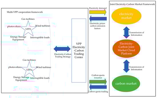
Figure 1.
Multiple VPPs participate in the operation framework of the electricity–carbon joint market.
In the joint electricity–carbon market, both markets optimize their operational strategies based on their respective energy attributes. To address the challenge of leveraging VPPs for electricity–carbon coordination, this study proposes a novel joint trading framework powered by cloud computing technology.
The framework enables VPPs to participate in market operations by uploading transaction data to a centralized platform. Within the VPP alliance structure, the cloud platform aggregates agreed-upon tariffs and power volumes from member VPPs. After processing these data via an information network, it determines the final transaction amounts.
To ensure accuracy, the platform dynamically updates electricity prices and carbon emission reductions in real time, reflecting current alliance demand. Finally, transaction results are distributed to each VPP through a secure communication network.
Within the VPP alliance framework, each member coordinates its internal power generation assets, renewable energy units, and energy storage systems in response to the upper market electricity demand. By simultaneously submitting generation plans and participating in carbon market transactions, members ensure compliance with emission requirements while optimizing resource utilization across interconnected regions. This coordinated approach enables the multi-VPP alliance to effectively participate in joint electricity–carbon markets, achieving optimal resource allocation through collective optimization that balances energy supply with environmental objectives [17].
2.1. Pre-Scheduling Within the VPP System
2.1.1. Pre-Scheduling Strategies Within the VPP System
Wind power and photovoltaic power, as important components of new energy generation, are characterized by randomness, volatility, and intermittency, making their output difficult to predict accurately. To better ensure the safe and stable operation of the power grid and enhance the capacity for absorbing new energy, wind power and photovoltaic power need to participate in the day-ahead generation dispatching of the power grid, so as to keep their output within a reasonable range and match the overall load demand of the system.
First, the day-ahead scheduling process is shown in Figure 2.
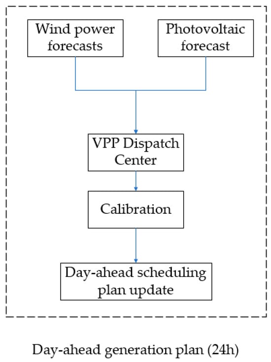
Figure 2.
Day-ahead generation plan flowchart.
Upon receiving wind and photovoltaic power forecast data, the grid dispatch center initiates a correction process to account for prediction inaccuracies inherent to renewable energy forecasting. The center employs an integrated approach combining historical performance data, meteorological correction models, and real-time grid operating conditions to refine the renewable generation forecasts. Concurrently, system operators incorporate load forecasts and conventional generation schedules from thermal to maintain overall system power balance.
Following this comprehensive adjustment process, the dispatch center revises the day-ahead generation schedule and updates the grid dispatch system with the corrected plan. These refined forecasts serve dual purposes: they establish reference output levels for renewable energy plants in the subsequent operating day while simultaneously providing critical input for real-time dispatch decisions. The updated schedule enhances operational reliability by better aligning anticipated renewable generation with actual system conditions.
The core of the intraday generation plan is based on load data and wind and solar forecast data and is updated in a high-frequency cycle to ensure the efficient consumption of new energy and the stable operation of the grid, and the specific process is shown in Figure 3.
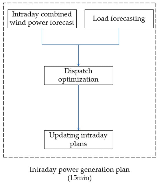
Figure 3.
Intraday movement control framework.
The intraday scheduling process begins with real-time load data acquisition. Grid loads exhibit dynamic fluctuations influenced by multiple factors, including temperature variations, industrial production cycles, and residential consumption patterns. To accurately predict near-term power demand, dispatch centers continuously monitor load data while employing short-term forecasting models for rolling updates.
Concurrently, wind and solar farms provide high-frequency intraday forecast updates, typically at 15 min intervals. These forecasts offer superior temporal resolution compared to day-ahead predictions and incorporate real-time meteorological data to enhance accuracy.
Wind power forecasts demonstrate particular stochastic characteristics, with output variability increasing significantly during strong wind conditions or rapid wind speed changes. These conditions often produce noticeably high-frequency oscillations in the power curve. Photovoltaic generation, while generally following more predictable diurnal patterns aligned with solar cycles, can still exhibit substantial variability during cloud cover transitions or sudden weather changes that affect solar irradiance.
The intraday real-time scheduling process framework is shown in Figure 4.
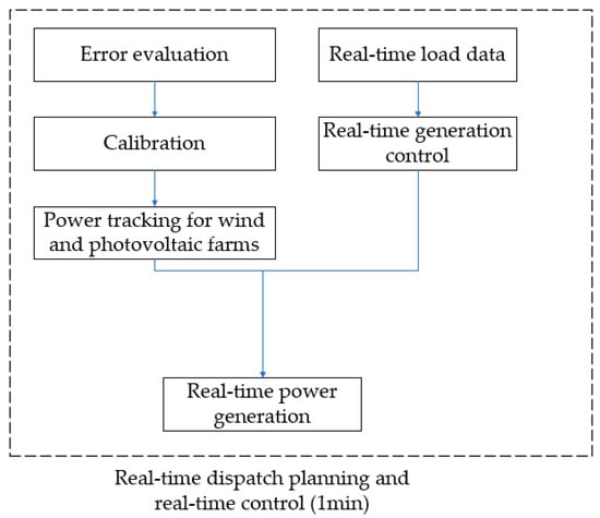
Figure 4.
Real-time scheduling framework.
The overall framework regarding pre-scheduling within VPPs is shown in Figure 5.
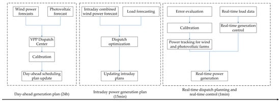
Figure 5.
Time-based wind and photovoltaic power dispatching framework.
2.1.2. Pre-Scheduling Model Based on Load Factor
Along with the access to renewable energy and various distributed energy sources in the power grid, the stability of the whole power system and the rational utilization of resources are facing serious challenges. In response to the serious phenomenon of wind and light abandonment in the existing system, it is necessary to adopt a suitable strategy to reduce the internal rate of wind and light abandonment and increase the rate of new energy consumption.
Pre-dispatch is performed based on the previous day’s load demand and market clearing results, and a method is proposed to measure the degree of consistency between the forecasted output and the load level during the dispatch period in terms of the load factor, and the standardized value of the VPP output during the dispatch period is calculated as shown in Equation (1):
where and represent the nominal value of the VPP output and the nominal value of the load signal at time t; represents the actual output of the i-th VPP at time t; represents the maximum output of the i-th VPP at time t; represents the actual value of the load demand at the node at time t.
Comparing the output and load of the VPP in the grid aims to calculate the deviation of the above two at a certain moment in time, which is calculated as shown in Equation (2):
Load tracking factor is defined as shown in Equation (3):
When the value of the calculation result is closer to 1, it means that at that moment in time, the VPP is in line with the load demand, and when the value is further from 1, it means that the output of the VPP is not in line with the load demand and internal scheduling is required.
The pre-scheduling of each VPP within the system begins with the value of the above load tracking factor, followed by pre-scheduling, calculated as shown in Equation (4):
where represents the scalar value of the scheduling quantity of the ith VPP at time t; represents the threshold value of the load tracking coefficient.
The significance of setting the threshold value is to prevent the VPP from having too large a difference between the output curve and the load curve at a certain point in time, which affects the amount of offer quotes within the whole VPP system and thus affects the revenues of the whole VPP alliance; thus, the minimum of the total number of dispatches and the maximum of the value of the dispatches in that time period can be taken as an objective function in this stage, and the ratio of the power inequality measure to the total load level is taken as a constraint to carry out the pre-scheduling.
2.2. Operational Modeling of Multi-VPP Cooperation Under Asymmetric Nash Negotiations
Among the VPPs selected in this paper, gas turbines, wind turbines, photovoltaics, energy storage, and part of the interruptible loads are mainly selected as the research objects. When participating in the operation of the multi-market, the VPP carries out cooperative transactions within the VPP to satisfy the needs of each internal equipment unit while optimizing the synergy with the other VPPs.
Multi-VPP Optimized Operational Model
The objective function is the total cost, which is mainly considered to be composed of fuel costs, electricity trading costs, carbon trading costs, and equipment maintenance costs, and is based on the minimization from the total cost as the objective function,
where represents the fuel cost of the i-th VPP at time t; represents the transaction cost of electricity for the i-th VPP at time t; represents the carbon transaction cost of the i-th VPP at time t; represents the operating and maintenance cost of the equipment of the i-th VPP at time t.
Fuel costs are dominated by the natural gas consumed by the gas turbines and fuel cells within the system. This is shown in Equation (6):
where represents the power produced by the gas turbine at time t; represents the power produced by the fuel cell at time t; represents the fuel consumption per unit of energy of the gas turbine; represents the fuel consumption per unit of energy of the fuel cell; represents the energy efficiency of the fuel cell at time t; represents the unit price of natural gas.
Electricity transaction costs mainly consist of transaction costs between individual VPPs and the rest of the VPPs in the system, as well as transaction costs with the higher-level grid. This is shown in Equation (7):
where represents the amount of electricity traded between VPPs; represents the cost of electricity traded between VPPs and the grid; represents the negotiated tariff between VPPs; represents the power flow between VPPs; represents the traded tariff between VPPs and the grid; represents the power flow between VPPs and the grid.
The cost of carbon emissions mainly consists of the cost of trading carbon allowances between VPPs and the higher-level energy centers. Each VPP entity has a certain amount of government-issued carbon allowances, and after completing the internal clearance of carbon allowances within its own system, it can choose to sell the excess carbon allowances to the higher-level energy centers or complete the trading of carbon allowances with the rest of the VPP system. This is shown in Equation (8):
where represents the cost of carbon trading between VPPs; represents the cost of carbon trading between VPPs and energy centers; represents the price of carbon allowances between VPPs; represents the volume of carbon traded between VPPs; represents the price of carbon between VPPs and energy centers; represents the volume of carbon traded between VPPs and energy centers; represents the amount of carbon allowances that are free of charge to VPPs; represents the actual carbon emissions of VPPs.
Also,
where represents the amount of electricity supplied to the internal load of the ith VPP at time t; represents the amount of electricity purchased from the grid by the ith VPP at time t; represents the output power of the gas turbine inside the ith VPP at time t; represents the carbon emissions per unit of electricity supplied by the ith VPP to the jth VPP at time t; , , and represent the fixed parameters set.
The equipment within the VPP mainly involves interruptible loads, energy storage, and gas turbines. The operation and maintenance costs of the equipment are also mainly centered around the above equipment. The energy storage element involves the charging and discharging process, with the corresponding charging and discharging equipment maintenance costs. The total cost function and the cost function of each piece of equipment are shown in Equation (10):
where represents the cost of the interruptible load; represents the cost of the storage device; represents the cost of the gas turbine; represents the interruptible load type parameter; represents the amount of interruption of the interruptible load; and represent the charging and discharging power of the storage device; represents the charging and discharging efficiency; represents the cost of the call of the storage device; , , and represent the fixed parameters of the setting.
2.3. Restrictive Condition
In this paper, the main body of the selected VPP, mainly selected gas turbines, wind turbines, photovoltaics, energy storage, and part of the interruptible load, for the study of the composition of the object, can be analyzed in various aspects of the transaction. This paper intends to study, in order to participate in the transaction of the multifaceted market, VPPs within cooperative transactions, to meet the needs of the internal units of each device at the same time and optimize synergies with the rest of the VPP to ensure the most optimal use of resources.
Power balance:
where represents the use of distributed energy in the i-th VPP at time t; represents the PV output in the i-th VPP at time t; represents the wind power output in the i-th VPP at time t.
Interruptible load constraints [18]:
where represents the maximum number of interruptions for the interruptible load; represents the amount of time the interruptible load has been in the interruptible state; represents the maximum interruptible time; represents the number of interruptions for the interruptible load; represents the interruptible limit; represents the state of the interruptible load.
Gas turbine constraints:
where represents he maximum value of the gas turbine output; represents the minimum value of the gas turbine output; represents the operating status of the gas turbine; represents the climbing constraint of the gas turbine.
Energy storage constraints:
where represents the charge state of the energy storage unit at time t; and represent the state quantity of the energy storage unit charging and discharging, where the state value is set to 0/1; represents the rated capacity of the energy storage unit; and represent the minimum and maximum values of the charging power of the energy storage unit; and represent the minimum and maximum values of the discharging power of the energy storage unit; and represent the minimum and maximum values of the charge state of the energy storage unit.
Price constraints:
where represents the price of electricity between VPPs; represents the price of electricity between VPPs and the grid; represents the price of carbon allowances between VPPs; and represent the minimum and maximum price of electricity between VPPs; and represent the minimum and maximum price of electricity between VPPs and the grid; and represent the minimum and maximum price of carbon allowances between VPPs.
In addition to satisfying the above price constraints, preventing degradation of the problem and direct trading of VPPs with the electricity market requires the following:
- (1)
- The price of electricity traded between VPPs has to be between the prices of electricity in the external market;
- (2)
- The price of carbon allowances traded between VPPs has to be between the prices in the carbon market.
The inequality constraints are satisfied as follows,
where represents the price of electricity sold to the grid by the VPP in the system at time t; represents the price of electricity purchased from the grid by the VPP in the system at time t; represents the price of carbon allowances sold to energy centers by the VPP in the system at time t; represents the price of carbon allowances purchased from energy centers by the VPP in the system at time t.
Considering the joint electricity–carbon market, the asymmetric Nash negotiation model is as follows,
where represents the cost of cooperative status; represents the cost of independent operation.
3. Model Solution
3.1. Upper-Level Model
In the upper clearance model, Equation (1) is used as the objective function, where the following constraints need to be satisfied.
where represents the power between node A and node B at time t; represents the set of branch circuits at node A; represents the set of power plants at node A; represents the simplest cost of the i-th VPP when it operates independently; represents the phase angle at node A; represents the phase angle at node B; represents the maximum value of the branch circuit currents between node A and node B; and represent the minimum and maximum values of the energy output from the power plant v; and represent the minimum and maximum values of the creeping ramp of the power plant v; represents the fact that at time t, represents the prediction of energy output of power plant v at time t.
3.2. Lower-Level Model
3.2.1. AA-ADMM Algorithm Flow
AA-ADMM uses the Anderson acceleration technique, which is an acceleration strategy based on the idea of the proposed Newton method. This method mainly utilizes a linear combination of historical iteration points to predict the next step, thus reducing the residuals.
AA-ADMM significantly improves the convergence speed and stability of traditional ADMM by introducing the Anderson acceleration technique. In nonlinear or non-convex optimization problems, the AA-ADMM algorithm uses historical information to fit a better search direction, which is able to bypass the local extrema, such as the sparse regularization problem in deep learning; in distributed optimization problems, AA-ADMM significantly reduces the communication overhead by reducing the number of iterations, such as the global model aggregation in federated learning [19].
The specific process of AA-ADMM is shown below:
- (1)
- Introduce primitive variables: x is a global variable and z is a local variable;Introduction of dyadic variables: λ is the Lagrange multiplier;Objective function: f(x) (market returns), g(z) (operating costs);Introducing constraints: ax + Bz = c, z ∈ Z;
Penalty coefficient ρ > 0, scale factor β ∈ (0,1] for the original and pairwise residuals, and number of memory steps m.
- (2)
- Initialization.Initial solutions: x0, z0, λ0.History queues: residual queue F = [], variable difference queue G = [].Set the convergence tolerance ϵ.
- (3)
- Iterative calculation.
Update the local variables while solving as shown in Equation (19):
Update the global variables as shown in Equation (20):
Calculate the unaccelerated dyadic variables as shown in Equation (21):
- (4)
- Anderson acceleration.
Calculate the current residuals as shown in Equation (22):
Update the history queue. Add fk to the residual queue F = [fk−m, …, fk]. Add the variable difference (Δλk= λk− λk−1) to the queue G = [Δλk−m, …, Δλk]. If the queue length > m, discard the oldest element.
Solve for the acceleration factors as shown in Equation (23):
α is obtained by solving the following linear system,
Update the pairwise variables,
- (5)
- Convergence judgment.
Check raw and pairwise residuals,
When all the above residuals are less than the convergence accuracy, then the algorithm terminates; otherwise, return to step (1).
3.2.2. Model Equivalent Transformation
The Nash negotiation model of multi-VPP cooperative game, which can be regarded as a non-convex nonlinear optimization model, is sometimes long or unable to converge due to the excessive number of iterations when solved directly. Drawing on the methods in the literature [20,21], the above problems are transformed:
- (1)
- Minimization of the operating cost of the multi-VPP system,
- (2)
- Revenue allocation based on the contribution of each VPP within the system.
Firstly, it is necessary to specify the contribution factor γi of each VPP as shown in Equation (28) [22]:
where represents the total number of VPPs in the system; represents the time, which takes the value of 24 h; represents the weight of VPP electricity transactions; represents the weight of VPP carbon transactions.
At the same time, the following constraints are satisfied:
After completing the calculation of the contribution factor, based on the contribution factor, the trading revenue allocation is calculated as shown in Equation (22):
where represents the optimal solution of the objective function in the previous problem.
3.3. Two-Layer Model Solving
After completing the model transformation, the solution is solved by yalmip and gurobi solvers in Matlab 2022b. After determining the trading consensus, construct the augmented Lagrangian function and optimize it [23,24]:
where and represents the Lagrange multipliers; and represents the penalization factor.
For the problem of minimizing the operation cost of the upper layer, the solution steps are as follows:
- (1)
- Set the maximum number of iterations to 200, the convergence accuracy to 10−3, the penalty factor to 10−4, and the rest of the initial values to 0.
- (2)
- For all the VPPs in the VPP coalition to be solved in sequential order, the kth iteration result is obtained for the first VPP from the rest of the VPPs (Pj1,k,t,Ej1,k,t), where j ∈ {2, 3, …, N}; the remaining i-th VPP obtains the k + 1st iteration result from the 1st, 2nd, 3rd, …, i − 1st VPP(Pji,k+1,t, Eji,k+1,t), where j ∈ {1, 2, 3, …, i − 1}; starting from i + 1, i + 2 … N VPPs obtain the kth result (Pj1,k,t,Ej1,k,t), where j ∈ {i + 1, i + 2 … N}; the rest of the collaborators obtain the result k + 1st result (Pji,k+1,t,Eji,k+1,t).
- (3)
- After completing one iteration of the computation, the Lagrange multipliers are updated, and the original and pairwise residuals are computed.
- (4)
- Determine the penalization factor.where and represent the penalty factor; represents the residual scale factor; and represent the step factor; represents the original residual; represents the pairwise residual.
- (5)
- Update the penalization factor.
- (6)
- Update the number of iterations k = k + 1.
- (7)
- Determine the convergence—if the iteration termination condition is satisfied, output the final result; otherwise, return to step 2 to re-calculate until the convergence condition is satisfied or the maximum number of iterations is reached.
After completing the upper model solution, the optimal solutions and from Problem (1) are substituted into the Nash model, and the augmented Lagrangian function is constructed and optimized to create the following model:
Therefore, regarding the problem of the internal revenue distribution of lower VPPs, the solution steps are as follows:
- (1)
- Set the maximum number of iterations to 200, the convergence accuracy to 10−3, the penalty factor to 10−4, and the rest of the initial values to 0.
- (2)
- Solve the problem for all the VPPs in the VPP coalition in order, and obtain the kth iteration result for the first VPP from the rest of the VPPs (π1i,ek,t,π1i,ck,t), where j ∈ {2, 3, …, N}; the remaining i-th VPP obtains the k + 1st iteration result from the 1st, 2nd, 3rd, …, i − 1st VPP(πji,e(k+1),t,πji,c(k+1),t), where j ∈ {1, 2, 3, …, i − 1}; starting from i + 1, i + 2 … N VPPs obtain the kth result (πji,ek,t, πji,ck,t), where j ∈ {i + 1, i + 2 …N}; the rest of the collaborators obtain the result k + 1st result (πji,e(k+1), t, πji,c(k+1),t).
- (3)
- Subsequently, the Lagrange multipliers and penalty factors are updated with the same steps as in Problem 1 until, finally, the convergence condition is satisfied or the maximum number of iterations is reached.
The overall solution flow of the model is shown in Figure 6.
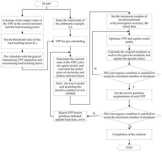
Figure 6.
Model solving diagram.
4. Case Analysis
4.1. Parameterization
The VPP consortium consists of three main VPPs, which are called VPP1, VPP2, and VPP3. The chosen computational period is 24 h, while the scheduling interval is 1 h. The types of generation in the grid include wind and thermal power, and the specific parameters of the generating units are shown in Table 1.

Table 1.
Generator sets and their parameters included in the selected case study.
The selected grid node topology is shown in Figure 7, the selected VPPs are connected to different nodes of the grid, and the distributed energy units and parameters inside the VPPs are shown in Table 2 and Table 3.
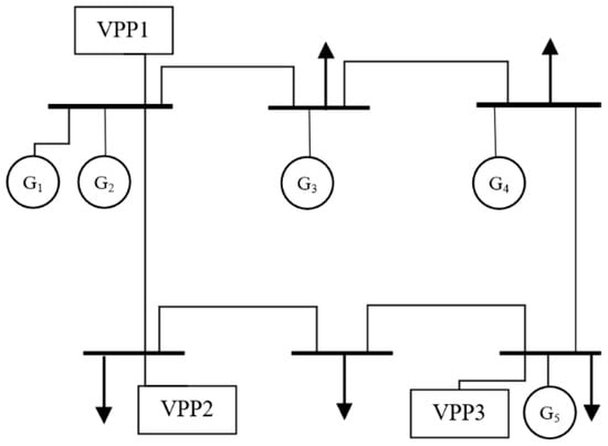
Figure 7.
Topology of power grid structure.
Table 2.
Distributed energy units and number of units included in the selected case study.
Table 3.
Specific parameters of distributed energy units within the VPP.
VPPs in the upper grid to purchase electricity and carbon quota prices are shown in Table 4. In order to make comparisons, first of all, the system of electricity trading set γe and carbon quota trading γc of the proportion of the system are set to 0.5; this is then followed by a comparison of the benefits under the different specific gravities.
Table 4.
Prices of products traded on the VPP and joint market under different time periods.
4.2. Analysis of Scenarios
According to the load data of the local grid, the appropriate load tracking coefficients are selected, and the pre-dispatch model is utilized to forecast the wind and PV power generation. The nodal loads based on the day-ahead market data, the forecasts of wind power, and PV power generation for each VPP are shown in Figure 8, Figure 9 and Figure 10.
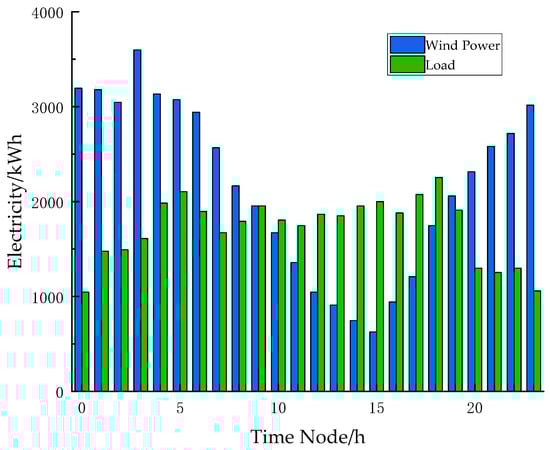
Figure 8.
Wind and load forecasts in VPP1 of selected case.
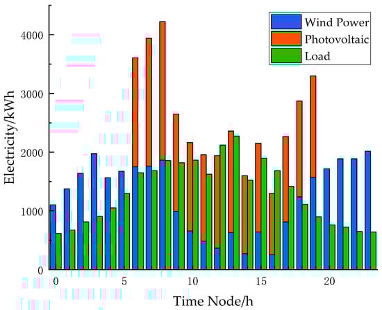
Figure 9.
Wind, PV, and load forecasts for VPP2 of selected case.
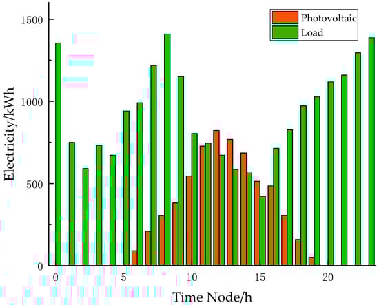
Figure 10.
PV and load forecasts for VPP3 for selected case.
In order to improve the prediction accuracy, it is necessary to consider applying the global optimization algorithm to optimize the prediction of wind and PV power generation, and after evaluating the index system, the pre-scheduling of the VPP is carried out to adjust the overall output of the VPP, and the adjustment results are shown in Figure 11.
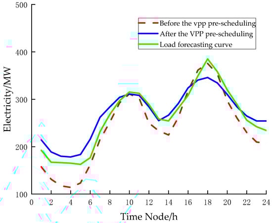
Figure 11.
VPP pre-scheduling curve.
In addition, we consider the impact of the spatial and temporal variability of carbon emission factors in VPPs on the participation of VPP coalitions in the joint electricity–carbon market and set up a two-scenario comparison to verify the conjecture.
Scenario 1: The carbon emission factor of each VPP is fixed without taking into account the effect of the carbon emission factor on the participation of the VPP alliance in the joint electricity–carbon market.
Scenario 2: The carbon emission factor of each VPP is calculated iteratively, taking into account the impact of the carbon emission factor on the VPP coalition’s participation in the joint electricity–carbon market.
The VPP operation under Scenario 1 and Scenario 2 was compared, as shown in Figure 12 and Figure 13.
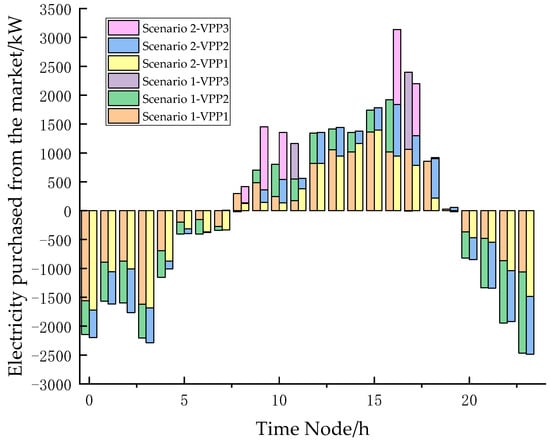
Figure 12.
VPP transactions with the grid in different scenarios.
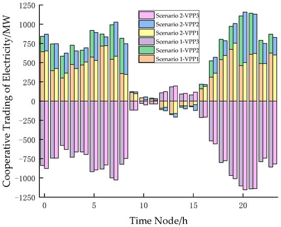
Figure 13.
Transactions of electrical energy within the VPP in different scenarios.
Electricity trading occurs between each VPP in the VPP alliance and the joint market, as well as the higher-level grid. Figure 12 represents the electricity trading between each VPP in the VPP alliance and the joint market, where the positive value indicates that the VPP purchases electricity from the joint market, and the negative value indicates that the VPP sells electricity to the joint market. Where Scenario 2 considers the impact of carbon emission factors on the participation of VPP alliances in the electricity–carbon joint market, in the 8:00–10:00 phase and the 16:00–20:00 phase, the amount of electricity purchased by VPP1 from the joint market decreases, while the amount of electricity purchased by VPP2 and VPP3 increases significantly. From the data, we can observe that the lower carbon emission factors lead to VPPs purchasing more low-carbon energy sources and provide additional low-carbon energy for other VPPs with higher carbon emission factors, thereby reducing the overall purchase of high-priced energy from the joint market by the VPP alliance. At the same time, the inclusion of cooperative trading between VPPs enabled VPPs to reduce their demand for high-carbon electricity, avoiding the addition of unnecessary carbon emissions while increasing the revenue of the VPP alliance.
In the case of the VPP alliance participating in the optimized operation of the electricity–carbon joint market, it is necessary to consider the profitability of each VPP within each alliance, and the following two strategies are used to verify the rationality of the asymmetric Nash bargaining method.
Strategy 1: The standard Nash bargaining revenue distribution method.
Strategy 2: The asymmetric Nash bargaining revenue allocation method, taking into account the contribution factor.
4.3. Analysis of Results
4.3.1. Analysis of the Operation of Multi-VPP Participation in the Electricity–Carbon Joint Market
The trading results of electricity and carbon allowances between VPP alliances are shown in Figure 14. Due to the inconsistency of the internal parameters of the selected VPPs, each VPP exhibits different electricity and carbon demands at different stages.
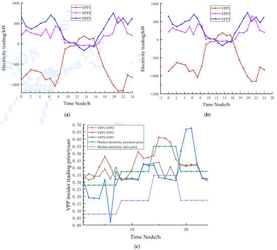
Figure 14.
Multi-VPP inter-electric–carbon trading results. (a) Inter-VPP electricity trading outcomes; (b) Inter-VPP carbon allowance trading outcomes; (c) Multi-VPP participation outcomes in the joint electricity–carbon market.
As can be seen from Figure 14c, in the 00:00–08:00 and 17:00–24:00 time periods, VPP1 and VPP2 provide additional renewable energy output for VPP3 due to the abundance of renewable energy within their own systems, which reduces the carbon emission cost within the alliance and thus helps reduce the operating cost of the entire VPP alliance. In the 10:00–15:00 time period, the overall load demand rises, in which VPP3’s PV unit output is larger and more abundant, while VPP1’s new energy output is smaller and VPP2’s new energy output is smoother but the load demand is too large, which results in the need to purchase high-priced electricity from the higher grid, so VPP1 and VPP2 prioritize purchasing electricity from within the VPP alliance to meet their internal needs. Therefore, VPP1 and VPP2 prioritize the purchase of electricity from within the alliance to meet the internal load demand.
For VPP3, it mainly uses photovoltaic units as a new energy source, and there is a positive correlation between its output and light intensity. Therefore, when the light intensity is insufficient and the output power cannot meet the internal demand, due to the high carbon emission factor of VPP3, VPP3 prioritizes purchasing power from the VPP alliance to fill the shortfall of its own power through the cooperation game with the alliance. Then, purchasing power is used from the higher grid to meet the demand for electricity, so that the cost of purchasing power and carbon emissions can be minimized.
Table 5 shows the benefits before and after each VPP collaboration.
Table 5.
Benefits of VPPs’ participation or non-participation in cooperative gaming.
As can be visualized in Table 5, comparing the revenues of each VPP and VPP alliance before and after the cooperation, the revenues are significantly improved. In the case of independent operation and direct trading in the electricity–carbon joint market, compared with participation in the cooperative game, each VPP prefers to trade within the alliance, which realizes the efficient use of energy and reduces its own operating costs.
Table 6 shows the carbon emissions and carbon emission costs of each VPP within the VPP alliance after participating in carbon market trading.
Table 6.
Comparison of carbon emissions of VPPs’ participation or non-participation in cooperative gaming.
Before the cooperation, the total VPP carbon emissions were 11.811 t, and the total cost was CNY −415; after participating in the coalition cooperation, the total VPP carbon emissions were 8.113 t, and the total cost was CNY −1341. The comparison of the two sets of data reveals that the total benefit increases by CNY 926 after participating in the cooperative game. Observing the performance of each VPP in the alliance, we can see that the carbon emissions of VPP1 and VPP2 have increased after the cooperation. However, due to the cooperation strategy within the coalition, VPP3’s demand for high-carbon electricity in the market has decreased, which can significantly reduce VPP3’s carbon emissions, thus obtaining significant low-carbon benefits. Thirdly, under different levels of emission reduction, the cooperation within the alliance can reduce the carbon emission cost and improve the overall benefit of the alliance. Therefore, based on the above research results, the cooperative operation of multi-VPPs is essential to reach the goal of low carbon emissions and plays a crucial role in promoting the growth of each economic entity.
4.3.2. Nash Bargaining Revenue Distribution Methods That Take into Account Product Contributions
Considering the uniqueness of each member in the VPP alliance, in order to ensure the relative reasonableness of the revenue of each VPP, it is necessary to consider the difference between the standard Nash bargaining model and the Nash bargaining revenue allocation method that takes into account the contribution of the product, and Table 7 shows the revenues of each VPP within the VPP alliance under the standard Nash bargaining revenue allocation.
Table 7.
Distribution of gains under standard Nash bargaining.
The standard Nash bargaining model assumes that all participants have symmetric bargaining power in a negotiation, meaning that the bargaining power of each party is considered equal. In the absence of external constraints or asymmetric factors, it allocates the total revenue of the coalition based on the expected revenue of each participant. The main advantage of this method is its simplicity and ease of calculation, but it does not take into account the actual differences in the contributions of the participants or changes in market conditions. In contrast, the asymmetric Nash bargaining revenue allocation method, which takes into account contribution factors, takes into account the actual contributions of different participants in the coalition and is flexible enough to respond to the impact of market or policy changes on different members. In this model, the weights of the participants are determined based on their contributions, and their bargaining power and contributions to the market can be taken into account in the revenue allocation. By introducing the contribution factor, it makes the revenue allocation of the coalition members more realistic.
Comparing Table 5 and Table 7, it can be seen that under the influence of revenue allocation strategy 2, the revenue of VPP1 and VPP3 is significantly higher than that of strategy 1, while the revenue of VPP2 shows a certain degree of decline. Analyzed from a comprehensive perspective, VPP1 has a larger share of renewable energy and therefore has a larger contribution to carbon trading in the VPP coalition. However, in the context of increased daytime loads, VPP3’s PV units, as part of renewable energy, also have a relatively high contribution to coalition cooperation. Ultimately, the revenue allocation is carried out through the combined contribution factor, which not only improves the effectiveness of the cooperation between VPP1 and VPP2 but also brings more economic benefits to both parties. However, distributing all the benefits equally within the framework of benefit allocation strategy 1 does not accurately reflect the contribution level of each participant. Therefore, when considering the respective contribution levels of the VPPs and the reasonableness of the revenue allocation, the revenue allocation strategy of asymmetric Nash bargaining appears more appropriate.
4.3.3. A Study of the Impact of the Proportional Weighting of Electric Carbon Trading
Electricity trading and carbon trading represent two different market mechanisms, and they contribute differently to the revenues of coalition members. Electricity trading mainly affects the trading relationship between producers and consumers, while carbon trading involves emission controls, environmental policies, and other factors. If the electricity market is in a tight state, electricity producers may face higher market demand and price pressure and the importance of electricity trading rises, at which time the weighting factor of electricity trading is increased so that electricity producers can gain more revenue; on the contrary, if the carbon price rises or the policy is tightened in the carbon trading market, carbon emitters, clean energy producers, etc., may benefit from it, and at which time the weighting factor of carbon trading can be increased to ensure that these market participants will not be affected. The weighting factor was used to ensure that these market participants receive a larger share of the benefits. Volatility and policy regulation in the power and carbon markets can affect the revenue contributions of all parties. Adjusting the weighting factors in response to policy changes or market price fluctuations can quickly reflect these changes and ensure that all parties receive a fair share of the benefits in the new market environment. For example, if the price of electricity rises and the profitability of power producers increases, they can be ensured to benefit from bargaining by increasing the weighting coefficient of electricity trading (γe > γc), i.e., it shows that the VPP alliance is more encouraging for members to trade in electricity and that the revenue approach determined by the Nash allocation method based on the contribution will be more favorable to the members who have a larger proportion of electricity trading. On the other hand, in the carbon pricing rising background, the benefit of carbon trading may increase significantly, by appropriately increasing the weight coefficient of carbon trading (γe < γc). Then, it represents the fact that the alliance encourages members to trade carbon allowances more, and it can enable those members who benefit from the carbon market to achieve more allocations.
In the asymmetric Nash bargaining revenue allocation method, the weighting coefficients of electricity trading and carbon trading can be flexibly adjusted to realize a fairer revenue allocation or a revenue allocation that is more in line with the actual market demand. Through this method, the revenue share of different members in the alliance can be precisely controlled to ensure that the revenue allocation can reflect the actual market situation and balance the interests of all parties, especially in the case of asymmetric bargaining power of all parties in the joint electricity–carbon market mechanism. Each coalition member has a corresponding uniqueness, resulting in them usually achieving different bargaining power. By flexibly adjusting the weighting factors, weaker members of the coalition (e.g., small power utilities or high emitters) can be helped to obtain more out of the negotiation. For example, if a member dominates the electricity market, the weighting factor for carbon trading can be increased moderately so that the interests of other members can be more protected and the distribution of benefits of the overall alliance can be balanced; if a member has an advantage in the carbon market (e.g., more carbon emission allowances), the benefits of the member can be increased by increasing the weighting factor for carbon trading.
Table 8 shows the benefits of the VPP alliance and among the members under different weighting coefficients in order to study the selection of appropriate weights for electricity trading and carbon quota trading at different stages of the VPP alliance to obtain greater benefits.
Table 8.
Changes in VPP returns with different proportional weights.
4.3.4. Convergence Analysis of the Adopted Algorithm
The alternating-direction method of multipliers is a classic optimization algorithm and is widely used in fields such as distributed computing, machine learning, and signal processing [25,26]. In the past, when solving the problem of internal optimization of VPPs, traditional ADMM might converge slowly or even fail to converge in non-convex problems. However, AA-ADMM uses historical information to fit a better search direction and can bypass local extremum points. In order to verify the superiority of the AA-ADMM algorithm, the solutions of the ADMM, A-ADMM, and AA-ADMM algorithms for the same problem are compared and analyzed.
To verify the effectiveness, computational convergence, and speed of the AA-ADMM algorithm, the computational convergence of AA-ADMM, A-ADMM, and the standard ADMM algorithm is compared. Problem 1 in the lower model is selected for solution comparison. Table 9 shows the convergence comparison of the three methods. The convergence performance of the algorithm is closely related to the step size selection, and the setting of the step-size parameter directly affects the iterative efficiency.
Table 9.
Comparison of the convergence of ADMM algorithms.
Studies show that improper step-size values (either too large or too small) will lead to an increase in computing costs, manifested as an increase in the number of iterations and an extension of computing time. The traditional ADMM algorithm is relatively sensitive to the step-size parameter, and its convergence speed fluctuates significantly with the change in step size. In contrast, the improved A-ADMM algorithm effectively reduces the algorithm’s dependence on the initial step size by introducing a step-size correction mechanism. Experimental data show that this method can maintain a stable convergence time under different synchronization size settings. The further optimized AA-ADMM algorithm adopts a dynamic penalty factor adjustment strategy, achieving a faster convergence speed while ensuring the robustness of the algorithm and demonstrating superior computing performance.
In the process of solving optimization problems, the convergence accuracy has an important influence on the performance of the algorithm. When the initial values are the same, different requirements for convergence accuracy will significantly affect the convergence speed, computational efficiency, and stability of the above three algorithms. Therefore, by changing the convergence accuracy, the influence of the convergence accuracy on the computational performance of the algorithm is studied. Table 10 shows the comparison of the computation time of these three algorithms under different convergence accuracy requirements.
Table 10.
The calculation time under different convergence accuracy requirements.
Under the requirement of low convergence accuracy, the linear convergence characteristic of the standard ADMM makes it perform stably under the requirement of low accuracy, and it can usually meet the convergence conditions within a small number of iterations. Because the influence of the initial step size is relatively small, even if the parameter selection is not ideal, the algorithm can still enter the stable convergence stage relatively quickly. Therefore, it is suitable for occasions where the quality requirements for the solution are not high but feasible solutions need to be obtained quickly. However, if the number of conditions of the optimization problem is poor, the convergence speed of ADMM may still be slow, and even oscillations may occur in the initial stage. Moreover, the linear convergence speed leads to a significant increase in the number of iterations of the algorithm under high-precision requirements, and the computational cost rises sharply. The selection of parameters is more sensitive. If the initial value does not match the problem, it may lead to convergence stagnation or residual oscillation. Even for pathological problems, ADMM may not meet the high-precision requirements.
For the A-ADMM algorithm, due to the adoption of momentum acceleration technology, it drops rapidly in the initial iterations, usually reducing the number of iterations by 30% to 50% compared with the standard ADMM. It has a low dependence on the initial value parameters. Even if fixed parameters are adopted, it can still show a good acceleration effect. It is particularly suitable for large-scale machine learning problems, where early rapid convergence is more important than high-precision solutions. However, for general convex or non-convex problems, it may degenerate into linear convergence in the later stage, and the acceleration effect will weaken. The adjustment requirements for parameters are higher. Unreasonable momentum weights may lead to divergence or oscillation.
On this basis, AA-ADMM fits the optimal direction through historical information and usually converges faster than ADMM at low precision. It has a low dependence on the initial parameters. Due to its strong adaptive adjustment ability, it is particularly prominent in nonlinear problems and can effectively reduce the number of initial iterations. The local superlinear convergence characteristic makes it significantly superior to ADMM and A-ADMM under high-precision requirements. It is particularly suitable for pathological problems (such as non-convex optimization). Traditional methods may stagnate, while AA-ADMM can still converge stably.
5. Conclusions
The bidding strategy for multi-VPP participation in the operation of the electricity–carbon joint market based on the carbon emission factor involved the pre-scheduling of each VPP main body in the stage with scheduling, pre-scheduling based on the load demand of the previous day and the results of the market clearing, and proposing a method to measure the degree of consistency between the forecasted output and the load level of the scheduling period in terms of the load coefficient; after that, utilizing the theory of carbon emission and taking into account the effect of the variability of the carbon emission factor, the two-layer game model was established. This two-layer game model was for multi-VPPs to participate in the electricity–carbon joint market, in which a cooperative game is used within the VPP coalition and following a revenue allocation method based on product contribution; finally, the model is solved using AA-ADMM to obtain the results. By calculating and analyzing the selected examples, the following conclusions are obtained:
- (1)
- The bidding strategy of multi-VPPs participating in the operation of the electricity–carbon joint market, taking into account the carbon emission factor, has an important guiding role for each VPP entity to carry out pre-scheduling, adjust its own power generation plan, call for internal resources, and deepen the cooperation among VPPs, thus reducing overall carbon emissions and taking into account the economic benefits while also considering the environmental benefits.
- (2)
- Utilizing the asymmetric Nash bargaining method to distribute revenues based on the contribution degree within the VPP alliance and reasonably distributing the revenues with reference to the contribution degree are conducive to the long-term and stable operation of the VPP alliance.
This paper assumes that members within a VPP alliance are able to collaborate seamlessly, but there are several challenges that may exist in actual practice. First, communication delays may lead to lags in real-time dispatch instructions, affecting the efficiency of the alliance’s response to grid demand. Second, data privacy issues may hinder the sharing of sensitive information, such as generation and load among members, especially in competitive markets where participants may conceal real data for commercial interests.
To address these issues in the future, this paper proposes the following directions: (1) the use of edge computing and distributed optimization algorithms to reduce the reliance on centralized communication, thereby reducing latency and improving robustness; (2) the use of federated learning or differential privacy techniques to achieve collaborative optimization while protecting data privacy; and (3) the consideration of resilient option contracts. The electricity market can introduce a “resilient capacity market”, where VPPs commit by signing contracts to provide backup capacity in extreme events and obtain long-term returns. Dynamic carbon footprint accounting is necessary during the post-disaster recovery stage, when the energy scheduling of VPP may rely on high-carbon resources. It is necessary to design dynamic carbon accounting rules, allowing for short-term high emissions but providing subsequent low-carbon compensation.
Author Contributions
Funding acquisition, D.H. and W.H.; methodology, D.H. and X.M.; software, X.M.; supervision, D.H.; writing—original draft preparation, J.Z.; writing—review and editing, J.Z., D.H., X.M., and W.H. All authors have read and agreed to the published version of the manuscript.
Funding
This research is supported by National Social Science Fund project (Grant number: 19BGL003) and State grid Shanxi Electric power company technology project (Grant number: 52053023001R).
Data Availability Statement
The original contributions presented in the study are included in the article, further inquiries can be directed to the corresponding author.
Conflicts of Interest
The authors declare no conflict of interest.
Abbreviations
The following abbreviations are used in this manuscript:
| VPP | Virtual Power Plant |
| ADMM | Alternating-Direction Multiplier Method |
| A-ADMM | Accelerated Alternating-Direction Multiplier Method |
| AA-ADMM | Accelerated Adaptive Alternating-Direction Multiplier Method |
| IL | Interruptible Load |
| ESS | Energy Storage System |
| GT | Gas Turbine |
| DER | Distributed Energy Resource |
| PV | Photovoltaic |
| WT | Wind Turbine |
References
- Peng, D.G.; Shui, J.J.; Wang, D.H.; Zhao, H. A review of virtual power plant research under the “dual carbon” background. Power Gener. Technol. 2023, 44, 602–615. [Google Scholar]
- Çolak, M.; Irmak, E. A state-of-the-art review on electric power systems and digital transformation. Electr. Power Compon. Syst. 2023, 51, 1089–1112. [Google Scholar] [CrossRef]
- Xia, X.; Wu, X.G.; Tao, Y.F.; Du, Q.; Ye, J.; Chen, Y.; Yang, L. Low-carbon operation strategy for virtual power plants considering spatio-temporal coupling characteristics of small hydropower. Zhejiang Electr. Power 2022, 41, 22–31. [Google Scholar]
- Li, R.; Wang, B.Q.; Peng, X.Z.; Lv, H.M.; Li, S.Y. Dynamic pricing and optimal scheduling of multiple virtual power plants based on Stackelberg game. Renew. Energy 2024, 42, 986–994. [Google Scholar]
- Chen, Y.; Wei, Z.N.; Xu, Z.; Huang, W.J.; Sun, G.Q.; Zhou, Y.Z. Joint optimal dispatch strategy for multiple virtual power plants under electricity market reform. Automat. Electr. Power Syst. 2019, 43, 42–49. [Google Scholar]
- Wang, K.; Xue, Y.; Shahidehpour, M.; Chang, Y.; Li, Z.; Zhou, Y.; Sun, H. Resilience-oriented two-stage restoration considering coordinated maintenance and reconfiguration in integrated power distribution and heating systems. IEEE Trans. Sustain. Energy 2024. [Google Scholar] [CrossRef]
- Rajasegharan, V.V.; Veena, P.; Ramesh, S.; Karthikeyan, G. Virtual power plant for optimizing power flow in large-scale distributed networks. Electr. Power Compon. Syst. 2023, 1–21. [Google Scholar] [CrossRef]
- Su, Z.P.; Wang, L.; Liang, X.Y.; Zeng, S.Q.; Yu, Z.W. Optimal scheduling of virtual power plants considering tiered carbon trading and integrated demand response. China Electr. Power 2023, 56, 174–182. [Google Scholar]
- Wang, Q.C.; Du, X.H.; Zhao, W.; Zhang, J.S.; Shang, Y.K.; Zahng, W.X.; Jia, Y.B. Bidding and scheduling strategy for virtual power plants participating in spot markets under carbon trading. Mod. Electr. Power 2024, 41, 152–160. [Google Scholar]
- Zhu, C.M.; Bao, G.; Xu, R.; Song, Z.; Liu, Y. Low-carbon economic analysis of a virtual power plant with wind and solar power considering the integrated flexible operation mode of a carbon capture thermoelectric unit. Int. J. Greenh. Gas Control 2023, 130, 104012. [Google Scholar] [CrossRef]
- Dong, L.; Tu, S.Q.; Li, Y.; Pu, T. Dynamic pricing and energy management for multiple virtual power plants based on meta-model optimization algorithm. Power Syst. Technol. 2020, 44, 973–983. [Google Scholar]
- Wang, H.; Jin, Z.R.; Fang, H.; Wang, Y.; Li, X.; Wang, B. Game-theoretic energy management model for virtual power plants based on dynamic pricing. South. Power Syst. Technol. 2023, 17, 101–108. [Google Scholar]
- Zhong, R.H.; Zhang, Y.C.; Zhu, S.; Xie, S.W. Collaborative low-carbon operation strategy between virtual power plant alliances and distribution networks based on peer-to-peer electricity-carbon trading. Power Syst. Technol. 2024, 48, 3554–3563. [Google Scholar]
- Shen, S.C.; Han, H.T.; Zhou, Y.Z.; Sun, G.Q.; Wei, Z.N.; Hu, G.W. A peer-to-peer electricity-carbon-reserve trading model for multiple virtual power plants based on conditional value-at-risk. Automat. Electr. Power Syst. 2022, 46, 147–157. [Google Scholar]
- Kang, C.; Zhou, T.; Chen, Q.; Wang, J. Carbon emission flow from generation to demand: A network-based model. IEEE Trans. Smart Grid 2015, 6, 2386–2394. [Google Scholar] [CrossRef]
- Feng, C.S.; Xie, F.R.; Wen, F.S.; Zhang, Y.B.; Hu, J.H. Design and implementation of a joint trading market for green certificates and carbon based on smart contracts. Automat. Electr. Power Syst. 2021, 45, 1–11. [Google Scholar]
- Cui, S.C.; Wang, Y.W.; Xiao, J.W. Peer-to-peer energy sharing among smart energy buildings by distributed transaction. IEEE Trans. Smart Grid 2019, 10, 6491–6501. [Google Scholar] [CrossRef]
- Tian, Y.; Lin, H.B.; Wang, H.B.; Fang, J.; He, J.X. An intelligent load optimization model for resilient distribution networks considering interruptible loads. Tech. Automat. Appl. 2024, 43, 56–59. [Google Scholar]
- Peng, Y. Research on Anderson Acceleration Method for Geometric Optimization. Ph.D. Thesis, University of Science and Technology of China, Hefei, China, 2021. [Google Scholar]
- Jiang, Y.; Zhang, J.; Zhang, T.; Liu, X.H.; Xue, Z.F.; Liu, Y.M.; Shi, J.J. Dynamic carbon emission responsibility factors for power systems. Proc. CSEE 2024, 44, 7024–7039. [Google Scholar] [CrossRef]
- Li, J.N.; Zhao, X.Z.; Zheng, Y.F.; Zhang, D.D. Optimal configuration of regional integrated energy systems considering energy sharing based on Nash bargaining. Power Syst. Prot. Control 2023, 51, 22–32. [Google Scholar]
- Yuan, G.L.; Liu, H.Q.; Yu, J.F.; Liu, X.F.; Fang, F. Combined heat and power optimal scheduling of virtual power plants with carbon capture thermal units. Proc. CSEE 2022, 42, 4440–4449. [Google Scholar]
- Wang, Q.; Wu, W.C.; Wang, B.; Wang, G.; Xi, Y.; Liu, H. Asynchronous decomposition method for the coordinated operation of virtual power plants. IEEE Trans. Power Syst. 2023, 38, 767–782. [Google Scholar] [CrossRef]
- Luo, P.; Zhou, H.B.; Xu, L.; Lv, Q.; Wu, Q.X. Day-ahead optimal scheduling of CCHP-based multi-microgrids using interval optimization. Automat. Electr. Power Syst. 2022, 46, 137–146. [Google Scholar]
- Xiong, H.; Luo, F.; Yan, M.; Yan, L.; Guo, C.; Ranzi, G. Distributionally robust and transactive energy management scheme for integrated wind-concentrated solar virtual power plants. Appl. Energy 2024, 368, 123148. [Google Scholar] [CrossRef]
- Li, S.; Wu, W.; Lin, Y. Robust data-driven and fully distributed Volt/VAR control for active distribution networks with multiple virtual power plants. IEEE Trans. Smart Grid 2022, 13, 2627–2638. [Google Scholar] [CrossRef]
Disclaimer/Publisher’s Note: The statements, opinions and data contained in all publications are solely those of the individual author(s) and contributor(s) and not of MDPI and/or the editor(s). MDPI and/or the editor(s) disclaim responsibility for any injury to people or property resulting from any ideas, methods, instructions or products referred to in the content. |
© 2025 by the authors. Licensee MDPI, Basel, Switzerland. This article is an open access article distributed under the terms and conditions of the Creative Commons Attribution (CC BY) license (https://creativecommons.org/licenses/by/4.0/).