A Federated Learning Algorithm That Combines DCScaffold and Differential Privacy for Load Prediction

Abstract

Accurate residential load forecasting plays a crucial role in optimizing demand-side resource integration and fulfilling the needs of demand-side response initiatives. To tackle challenges, such as data heterogeneity, constrained communication resources, and data security in smart grid load prediction, this study introduces a novel differential privacy federated learning algorithm. Leveraging the federated learning framework, the approach incorporates weather and temporal factors as key variables influencing load patterns, thereby creating a privacy-preserving load forecasting solution. The model is built upon the Long Short-Term Memory (LSTM) network architecture. Experimental results demonstrate that the proposed algorithm enables federated training without the need for sharing raw load data, facilitating load scheduling and energy management operations in smart grids while safeguarding user privacy. Furthermore, it exhibits superior prediction accuracy and communication efficiency compared to existing federated learning methods.

1. Introduction

The modern power system is a typical complex intelligent network integrating information, physics, society, and big data, with renewable energy as its main component [1]. New technologies, for example, demand response, electricity retailers, load aggregators, digital twins, and virtual power plants, which are continuously being introduced, making power loads exhibit more complex and dynamic new characteristics and forms [2]. Load forecasting is a foundational task for the new power system, playing a crucial role in the planning, operation, control, and scheduling of future smart grids.

In 2022, the Chinese government stated that data [3], as a new factor of production, are the foundation of digitalization, networking, and intelligence. The relevant document emphasizes strengthening data security throughout the entire process of data supply, circulation, and usage. As a critical national infrastructure, grid data in the modern power system is closely related to national security and socio-economic development. Ensuring data privacy and security in the modern power system is crucial to its network security [4].

Traditional big data mining methods in the power grid rely on central servers to integrate multi-party data for model training, which raises multiple issues such as data privacy, security, and client rights protection. Additionally, the system’s vulnerability to attacks inevitably threatens data security. In the context of privacy protection, if users choose to store data locally on their client devices, active distribution grid operators will not be able to access their meter data, leading to a significant reduction in the accuracy of load forecasting. Given the emphasis on data privacy protection, accurately predicting users’ power load without directly sharing local data becomes crucial. Federated learning (FL) [5,6] provides a new approach for privacy-preserving load forecasting. FL is a distributed machine learning framework that keeps data local, allowing multiple clients (e.g., edge devices) to collaboratively train machine learning models. This is especially useful in vulnerable IoT environments. In FL algorithms, users retain load data locally and only upload the trained load characteristic parameters to the server. FL reduces the risk of privacy leakage by not sharing data between devices and offers a new solution for data island.

However, existing FL-based load forecasting algorithms still have the following shortcomings:

(1)

Data quality is an important foundation for load forecasting in power systems. Existing methods often assume that users’ load data are independent and identically distributed (IID) and use federated stochastic gradient algorithms or Federated Averaging algorithms for model training. While the data from different users is independent, the assumption of identical distribution does not hold true in practice, which affects the predictive accuracy of the model.

(2)

Although the training data for the FL model does not leave the local device, mitigating the data security issues inherent in traditional centralized learning, it still requires uploading model parameter updates. Attackers can infer users’ sensitive information from the uploaded model parameters, making it difficult to ensure data privacy [7].

(3)

Since updated model parameters need to be continuously exchanged between local users and the server, when the number of users is large and the number of convergence rounds is high, this communication overhead can lead to increased network latency and even packet loss. This severely impacts model performance and can degrade the user experience for those participating in training, making them reluctant to engage in model learning, which inevitably affects the forecasting results [8].

In this context, a plethora of novel federated learning (FL) algorithms were successively introduced. To enhance communication efficiency and reduce the size of transmitted model updates, a variety of data compression techniques, including quantization [9], sparsification [10], model pruning [11], and knowledge distillation [12], are proposed. Reference [13] introduced a lazily aggregated quantized gradient mechanism, which dynamically adjusts communication frequency based on update significance. Reference [14] explored the issue of energy prediction in smart grids using FL by integrating an inner product function encryption method with a CAT (Change and Transmit) communication strategy, significantly improving communication efficiency within acceptable algorithmic accuracy, thereby saving communication costs and achieving a trade-off between model performance and communication bandwidth. Reference [15] bolstered the robustness of the FL framework against malicious attacks through gradient quantization and differential privacy (DP) techniques, safeguarding the security of FL models and architecture. Reference [16] introduced a DP stochastic gradient descent algorithm for training neural networks under a modest privacy budget. Reference [17] proposed a DP FL algorithm, conducted an analysis of its performance, and extended this to federated settings by analyzing the trade-offs between privacy and model utility. Clustering federated algorithms [18] and personalized federated learning [8] offered solutions to data heterogeneity issues from the perspective of model frameworks. Optimization algorithms with adaptive learning rates, such as FedAdagrad, FedYOGI, and FedAdam, have proven effective in handling non-IID data in FL [8]. Reference [19] presented a deep learning-based quantile regression method for interval prediction of electric load. Karimireddy S P et al. introduced SCAFFOLD [20], which leverages variance reduction techniques and employs control variables to rectify client drift in local updates. Building upon this, reference [21] further enhanced SCAFFOLD with differential privacy guarantees, providing a comprehensive solution for privacy-preserving federated learning on heterogeneous data. In addition to data privacy issues, other network security issues such as data poisoning and evading attacks are also receiving increasing attention [22]. For an overview of FL algorithms and future research directions, one may refer to [23,24].

While these approaches have made significant strides, they typically focus on individual challenges rather than a holistic integration of communication efficiency, privacy protection, and data heterogeneity. To this end, our work bridges this gap by proposing a unified framework that simultaneously addresses all three aspects. To address the aforementioned limitations, this paper first proposes a novel algorithm, DCScaffold, based on the classic Stochastic Controlled Averaging Algorithm (SCAFFOLD), which can effectively enhance forecasting performance. Furthermore, this paper introduces a novel differential privacy-preserving federated learning algorithm. This approach aims to improve the algorithm’s applicability by considering three key aspects: communication efficiency, privacy preservation, and non-IID data. It utilizes weather and temporal factors as parameters relevant to load, establishing a federated learning framework specifically designed for load forecasting with a strong emphasis on safeguarding user data privacy. The Long Short-Term Memory (LSTM) network is employed to construct the load forecasting model, which elucidates the operational characteristics of the load and offers support for decision-making in smart grid load scheduling and energy management. Empirical evaluations demonstrate that the proposed algorithm outperforms existing federated algorithms in terms of prediction accuracy and communication efficiency.

2. Materials and Methods

2.1. Federated Learning Model

Federated Averaging (FedAvg) is a foundational algorithm in federated learning, characterized by its straightforward yet efficient workflow. The process begins with the central server initializing a global model and distributing it to all participating clients. Each client then performs local training using its own data, updating the global model over multiple iterations to produce a locally optimized version. These updated model parameters are subsequently transmitted back to the central server, which aggregates them to form a new global model. The updated global parameters are then broadcast to all clients, initiating the next round of training. Through iterative execution of these steps, the global model is progressively refined. FedAvg offers a simple yet robust approach to model aggregation in federated learning, serving as a cornerstone for subsequent algorithmic advancements. The classic federated learning architecture employs a star topology, as illustrated in Figure 1, comprising a single server and multiple clients, where ${\theta }_i^k$ represents the model parameters of the ith client during the tth communication, and ${\theta }^{k+1}$ represents the aggregated global model parameters and the model parameters of the client during the tth communication.

Equation (1) represents the loss function on the ith local client [17,25].

$$\underset{\theta }{\min }{J}_i(\theta )={\displaystyle \frac{1}{\left|D_i\right|}}{\displaystyle \sum _{j=1}^{\left|D_i\right|}L(\theta ,{\xi }_j)},$$

(1)

where θ is the model parameter ${\xi }_j\in D_i$. For data samples, $D_i$ is the client dataset and L denotes the loss function. The summation is taken over index j. In the process of deep learning, we need to minimize the loss function J(θ). The global loss function is defined by Equation (2) [26].

$$\underset{\theta }{\min }J(\theta )={\displaystyle \sum _{i=1}^{\left|S\right|}\frac{\left|D_i\right|}{{\displaystyle \sum _{i=1}^{\left|S\right|}\left|D_i\right|}}{J}_i(\theta )},$$

(2)

where S represents the collection of clients drawn to participate in the training. During the training process, the client uses the stochastic gradient algorithm to update the model parameters, as given by Equation (3).

$${\theta }_i^{k+1}={\theta }_i^k-\eta \nabla J_i(\theta ).$$

(3)

For the learning rate η, Equation (4) represents an update performed by the server to the global model, specifically as follows:

$${\theta }^k={\displaystyle \sum _{i=1}^{\left|S\right|}{\frac{\left|D_i\right|}{{\displaystyle \sum _{i=1}^{\left|S\right|}\left|D_i\right|}}}_i{\theta }_i^k}.$$

(4)

Without loss of generality, we assume that the number of clients is n and that each client’s local dataset consists of m data points.

2.2. Differential Privacy

Differential privacy is a framework, which essentially provides privacy protection for the data by adding somewhat distributed noise to the data and strictly defines the intensity of privacy protection. Two datasets, D,D’, only one record apart is called two adjacent datasets. Differential privacy ensures that the same query operation is performed in any two adjacent datasets, and the query results are basically the same, that is, the output results are insensitive to changes in a single record in the dataset. The formal definition of differential privacy is as follows:

Definition 1.

Differential privacy [24]. For a randomization mechanism $M$, its defined domain is Dom(M), and the value domain is Range(M). If the randomization mechanism $M$ for any two adjacent datasets $D,D^{\prime }\subseteq Dom(M)$, $O\subseteq Dom(M)$ is satisfied, the following occurs:

$$\mathrm{P}\mathrm{r}[M(D)\in O]\le e^{\epsilon }\mathrm{P}\mathrm{r}[M(D^{\prime })\in O]+\delta .$$

Then, $M$ is satisfied $(\epsilon ,\delta )-DP$, where the parameter $\epsilon$ is a privacy protection budget used to measure the degree of privacy protection.

Definition 2.

Global sensitivity [27]. For a query function on a given dataset $f:D\to R^a$, whose input is a dataset, and the output is a d-dimensional real vector. The global sensitivity of f is defined as follows:

$$\Delta f={\max }_{D,D^{\prime }}{‖f(D)-f(D^{\prime })‖}_l,$$

where D,D’ is arbitrary two adjacent datasets, with l representing the vector norm of measured distance. In the following section, the value is below l = 2.

Zero-Concentrated Differential Privacy, zCDP, is a new form of differential privacy relaxation that reduces attention to individual query privacy losses during computation while increasing the cumulative loss probability bound from the usual $(\epsilon ,\delta )-DP$. In contrast, the privacy loss calculated by multiple iterations provides a clearer and more accurate analysis. zCDP’s definition is as follows.

Definition 3.

zCDP [28]. For any two adjacent datasets D,D’ and α > 1, the randomization mechanism M satisfies ρ-zCDP, if and only if the following occurs:

$$D_{\alpha }\left(\mathcal{M}(D)\Vert \mathcal{M}(D^{\prime })\right)={\displaystyle \frac{1}{\alpha -1}}\log \left(E\left[e^{(\alpha -1)L^{(O)}}\right]\right)\le \rho .$$

where $D_{\alpha }\{M(D)||M(D)\}$ indicate α-Renyi distance among M(D) and M(D’), and $L^{(O)}$ represents the results of the operation is $O$. Mechanism M produces the loss of privacy in adjacent datasets D and D’, where the following occurs:

$$L_{\left(\mathcal{M}(D)‖\mathcal{M}(D^{\prime })\right)}^{(O)}=\log {\displaystyle \frac{\mathrm{Pr}(\mathcal{M}(D)=O)}{\mathrm{Pr}(\mathcal{M}(D^{\prime })=O)}}.$$

.

The conclusions concerning zDCP can be summarized as follows.

Lemma 1 ([28]).

The Gaussian mechanism, which returns $f(D)+N(0, {\Delta }^2(f){\sigma }^{2}I)$, satisfies $(1/2{\sigma }^2)-z\mathrm{CDP}$.

Lemma 2 ([28]).

Suppose there are k types of mechanisms M₁,M₂,…M_k, and each M_i (for i = 1,2,…k) satisfies ρ_i-zCDP. Then, the composition of these mechanisms satisfies  $\left({\displaystyle \sum _{i=1}^k{\rho }_i}\right)-zCDP$.

Lemma 3 ([29]).

Suppose mechanism M is composed of a series of adaptive randomization mechanisms M₁,M₂,…M_E, and M_i (i = 1,2,…k) satisfies ρ_i-zCDP. When the dataset D is randomly split into D₁,D₂,…D_E, the mechanism $M(D)=\left(\begin{array}{c}{M}_1(D_1),M_2(D_2),\cdots ,M_B(D_B)\end{array}\right)$ meet $\underset{i}{max}{\rho }_i-zCDP$.

Lemma 4 ([28]).

Suppose mechanism M satisfies ρ-zCDP, then to arbitrary $\delta >0$, M satisfies $\left(\begin{array}{c}\rho +2\sqrt{\rho log(1/\delta )},\delta \end{array}\right)-DP$.

While $(\epsilon ,\delta )-DP$ provides rigorous privacy guarantees, its composition properties for iterative algorithms like federated learning may lead to overly conservative privacy budget estimations. zCDP offers a refined analysis framework that enables tighter composition bounds for multiple iterations. This is particularly advantageous in federated learning scenarios where model updates are aggregated over numerous communication rounds. By leveraging zCDP, we achieve more precise tracking of cumulative privacy loss while maintaining compatibility with Gaussian noise mechanisms. Furthermore, zCDP provides a smoother conversion to $(\epsilon ,\delta )-DP$ guarantees through Lemma 4, allowing for direct comparison with traditional privacy accounting methods. The adoption of zCDP therefore balances computational tractability and tight privacy analysis for our multi-round differentially private federated learning framework. zCDP’s definition is as follows.

3. Algorithm

3.1. Core Idea

This paper studies the collaborative work issues and privacy protection challenges faced by multiple data collectors in the process of power load forecasting. Each user in the power grid independently owns their electricity load data and is unwilling to directly share their raw data. Therefore, when it is necessary to complete load forecasting based on the electricity consumption data of all users, using a federated learning framework is a reasonable choice to address this issue.

3.2. DCScaffold Algorithm

SCAFFOLD is an improvement of the FedAvg algorithm. In federated learning, non-IID typically refers to the situation where the distribution of data is independent, but the data collection does not necessarily follow the same sampling method. Data in federated learning nodes is often generated in a non-IID manner and stored locally. Due to the differences in distribution characteristics between non-IID and IID data, training models on non-IID data may result in significant bias, leading to reduced efficiency and accuracy in federated learning, and it may even cause the federated learning algorithm to fail to converge. Therefore, research on non-IID data is crucial.

SCAFFOLD addresses heterogeneous data that is not independently and identically distributed (non-IID) by employing variance reduction techniques and using control variables to effectively correct client drift in client updates. In SCAFFOLD, control variables are set for each client and also for the server, containing directional information about model updates. By adding correction terms to local model updates on the client side, it effectively overcomes gradient discrepancies, thereby alleviating client drift. Each training round of the algorithm consists of three parts. First, clients perform local updates on model parameters using the mini-batch gradient algorithm. Then, clients update the local control variables and upload the model parameters. Finally, the server aggregates the local updates and updates the global model.

SCAFFOLD can provide better model utility in federated learning scenarios with non-IID data and has a faster convergence speed. However, because SCAFFOLD requires both model parameter updates and control variable updates to be uploaded in each round of global model aggregation, it significantly increases the communication burden of SCAFFOLD.

Although SCAFFOLD avoids directly exposing the raw data of local clients and provides some protection for data privacy, a risk of privacy leakage still exists. For honest but curious servers or participants, while they can train according to the model protocol without intentionally injecting erroneous information, they may be curious about the privacy information of clients and thus infer clients’ private information from the communicated model parameters, leading to privacy breaches.

To address these issues, this paper proposes an improved algorithm, DCScaffold. Based on SCAFFOLD, and to ensure the privacy security of client data while reducing the communication costs between clients and the central server in federated learning, we introduce a differential privacy mechanism and a CAT strategy. Additionally, we appropriately increase the local computation workload in each training round, which can effectively reduce communication overhead while protecting data privacy. By employing variance reduction techniques, we effectively alleviate client drift.

CAT (Communication-Aware Thresholding) is an event-triggered communication mechanism designed to optimize federated learning processes. The core principle of CAT is to reduce communication overhead by selectively transmitting only those local model parameters that exhibit significant changes compared to the previous round. Specifically, during each training round, the updated model parameters are compared with those sent in the last round, and only parameters whose absolute percentage change exceeds a predefined threshold are communicated to the server. A higher threshold enhances communication efficiency but may introduce larger errors in the transmitted parameters, potentially impacting the global model’s predictive performance. In Section 4, we explore the trade-offs between model performance and communication efficiency under varying thresholds through numerical experiments. Additionally, the CAT strategy helps mitigate issues such as overtraining and local optima, thereby enhancing the stability and robustness of the federated learning model.

The improved algorithm DCScaffold proposed in this paper is based on SCAFFOLD and comprehensively considers the heterogeneity of users’ electricity load data, privacy security, and communication bandwidth during model training. In the r-th training round, first, the client samples mini-batch data to compute gradients, then add Gaussian noise and correction terms c^r−1-c_i^r−1 to update the local model parameters. The Gaussian noise that complies with the privacy budget further protects the privacy of client data, and the introduction of correction terms effectively alleviates client drift caused by data heterogeneity. After updating the local model parameters K times, local control variables are updated. Based on the CAT strategy, the updated parameters are compared with the trigger threshold, and if communication is triggered, the local updates are uploaded. This effectively saves communication bandwidth. After receiving the client updates, the server uses gradient optimization for global aggregation updates, producing the next round of the global model. If the updates received from the clients are empty, the server repeats the use of the previous round’s client parameters for the global update.

Remark 1.

The proposed DCScaffold algorithm distinguishes itself from existing methods in three key aspects. First, unlike traditional Federated Averaging (FedAvg) and adaptive gradient methods (e.g., FedAdaGrad), which primarily focus on communication efficiency or non-IID data handling, DCScaffold integrates differential privacy (DP) mechanisms directly into the SCAFFOLD framework, ensuring robust privacy guarantees without compromising model utility. Second, compared to existing DP-based federated learning approaches [16,21], DCScaffold introduces a novel CAT strategy that dynamically adjusts communication frequency based on parameter updates, significantly reducing communication overhead while maintaining prediction accuracy. Third, while SCAFFOLD [20] addresses client drift through control variables, DCScaffold enhances this by incorporating local differential privacy noise and adaptive correction terms, which not only mitigate data heterogeneity but also provide stronger privacy protection against inference attacks. These innovations collectively enable DCScaffold to achieve a superior balance among communication efficiency, privacy preservation, and non-IID data handling, addressing the limitations of existing methods in a unified framework.

The specific process is summarized in Algorithm 1.

Algorithm 1 DCScaffold Algorithm

Input: Communication rounds R, Number of local model updates K, Global model initial value $x^0$ and global control change. Quantity initial value $c^0$, global learning rate ηg, gradient trimming threshold C, CAT threshold H, temporary storage value ${\left\{T{g}_i\right\}}_{i=1}^n$, local control variable initial value ${\left\{c_i^0\right\}}_{i=1}^n$, local learning rate ηl.

Output: Model parameters $x^R$

1: for each round $r=1,\dots ,R$ do:

2:             Sample clients $S\subseteq \{1,\dots ,n\}$

3:             Communicate $(x^{r-1},c^{r-1})$ to all clients $i\in S$

4:             On client $i\in S$ in parallel do:

5:                     Initialize local model $y_i^0\leftarrow x^{r-1}$

6:                     for $k=0,\dots ,K-1$ do:

7:                            Sample a mini-batch $X_i\subseteq D_i$ of size $\lambda$ and compute gradient $g(y_i^k)\leftarrow (1/\lambda ){\displaystyle \sum _{{\xi }_i\in X_i}\nabla L(y_i^k,{\xi }_i)}$

8:                            Clip gradient:

$\overline{g}(y_i^k)\leftarrow g(y_i^k)/\max (1,{\displaystyle \frac{{‖g(y_i^k)‖}_2}{C}})$

9:                            Sample DP noise ${\gamma }_i^k\sim N(0,{\sigma }^{2}I)$

10:                            $y_i^{k+1}\leftarrow y_i^k-{\eta }_l(\overline{g}(y_i^k)-c_i^{r-1}+c^{r-1}+{\gamma }_i^k)$

11:                   end for

12:                       $c_i^{+}\leftarrow c_i^{r-1}-c^{r-1}+{\displaystyle \frac{1}{K{\eta }_l}}(x^{r-1}-y_i^K)$

13:                   $(\Delta y_i^r,\Delta c_i^r)\leftarrow (y_i^K-x^{r-1},c_i^{+}-c_i^{r-1})$ 14:                     $c_i^r\leftarrow c_i^{+}$

15:                 if  $\left|{\displaystyle \frac{\Delta y_i^r}{x^{r-1}}}\right|\times 100\%\ge H$

16:                     Upload $(\Delta y_i^r,\Delta c_i^r)$ to server

17:                 else

18:                         $(\Delta y_i^r,\Delta c_i^r)\leftarrow None$

19:                         Upload $(\Delta y_i^r,\Delta c_i^r)$ to server

20:                 end on client

21:                 Server aggregates do:

22:                         if $(\Delta y_i^r,\Delta c_i^r)=None$

23:                                 $(\Delta y_i^r,\Delta c_i^r)\leftarrow T{g}_i$

24:                     else:

25:                                 $T{g}_i\leftarrow (\Delta y_i^r,\Delta c_i^r)$

26:                         $(\Delta x^r,\Delta c^r)\leftarrow {\displaystyle \frac{1}{\left|S\right|}}{\displaystyle {\sum }_{i\in S}(\Delta y_i^r,\Delta c_i^r)}$

27:                         $x^r\leftarrow x^{r-1}+{\eta }_g\Delta x^r$ and $c^r\leftarrow c^{r-1}+{\displaystyle \frac{\left|S\right|}{n}}\Delta c^r$

28: end for

3.3. Privacy Analysis

Differential privacy is introduced to solve differential attacks and prevent the honest but curious server or participant from stealing the sensitive privacy information of the client according to the shared information.

Theorem 1.

In Algorithm 1, for the clients i involved in the training with local datasets D_i, random draw small batch samples without replay with a size of λ. Suppose the number of times client i participates in training and uploads updates in R rounds of learning as R_i, then for the client i, Algorithm 1 satisfies $({\epsilon }_i,\delta )-DP$, where the following occurs:

$${\epsilon }_i={\displaystyle \frac{2R_{i}K{C}^2}{m\lambda {\sigma }^2\left|S\right|}}+2\sqrt{{\displaystyle \frac{2R_{i}K{C}^2}{m\lambda {\sigma }^2\left|S\right|}}\log {\displaystyle \frac{1}{\delta }}}$$

.

Proof of Theorem 1.

In the following, we first compute the sensitivity of the gradient based on gradient clipping techniques. Then, we compute the sensitivity of the uploaded local model to further capture the zCDP guarantee of each communication round. Finally, we show that Algorithm 1 satisfies $({\epsilon }_i,\delta )-DP$ for device i after R communication rounds. □

To the client i, suppose that in two adjacent datasets X_i and X_i’, only data j is different, ${\xi }_j\ne {\xi }_j^{\prime }$, so the following occurs:

$$\begin{array}{c}{‖\overline{g}(y_i^k)(X_i)-\overline{g}(y_i^k)(X_i^{\prime })‖}_2={\displaystyle \frac{1}{\lambda }}‖\overline{g}(y_i^k)({\xi }_j)-\overline{g}(y_i^k)({\xi }_j^{\prime })‖\\ \le {\displaystyle \frac{2C}{\lambda }}\end{array}.$$

(5)

Note that when no Gaussian noise is added, there is the following:

$$\begin{array}{c}{y}_i^K=y_i^{K-1}-{\eta }_l\overline{g}(y_i^{K-1})-{\eta }_l(c^{r-1}-c_i^{r-1})\hfill \\ =y_i^{K-2}-{\eta }_l\overline{g}(y_i^{K-2})-{\eta }_l\overline{g}(y_i^{K-1})-2{\eta }_l(c^{r-1}-c_i^{r-1})\hfill \\ =\cdots \hfill \\ =y_i^0-{\eta }_l\overline{g}(y_i^0)-{\eta }_l\overline{g}(y_i^1)-\cdots -{\eta }_l\overline{g}(y_i^{K-1})-K{\eta }_l(c^{r-1}-c_i^{r-1})\hfill \end{array}.$$

(6)

And known from references [21], the following occurs:

$$\begin{array}{c}\Delta (y_i^K)={\eta }_l‖\overline{g}(y_i^0)(X_i^0)-\overline{g}(y_i^0)(X_i^{0\prime })+\overline{g}(y_i^1)(X_i^1)-\overline{g}(y_i^1)(X_i^{1\prime })+\cdots \hfill \\ +\overline{g}(y_i^{K-1})(X_i^{K-1})-\overline{g}(y_i^{K-1})(X_i^{K-1\prime })‖\hfill \\ \le {\displaystyle \frac{2{\eta }_{l}KC}{\lambda }}\hfill \end{array}.$$

(7)

From Equation (5) and Lemma 1, under Algorithm 1, each participating client in one local iteration would satisfy $2{\mathrm{C}}^2/{\lambda }^2{\sigma }^2-\mathrm{zCDP}$, and during a round of local iteration process, the total number of visits to the local datasets is $K\lambda /m$. According to Lemma 2 and Lemma 3, participants in a round of local iterative client satisfies $2K{C}^2/m\lambda {\sigma }^2-\mathrm{zCDP}$. Combinates Formula (7) and Lemma 1, after the r-round training of Algorithm 1, all client satisfies $2K{C}^2/m\lambda {\sigma }^2\left|S\right|-\mathrm{zCDP}$ and the times the client i participates in training and uploads updates in R round learning is R_i. Then, in the whole learning process, client i realizes $2R_{i}K{C}^2/m\lambda {\sigma }^2\left|S\right|-\mathrm{zCDP}$. From Lemma 4, the theorem is proved.

4. Federated Learning Power Load Forecasting Model Construction

4.1. The Factors of the Load

The key challenge for household load forecasting lies in the high volatility and uncertainty of load profiles. Electric load is influenced by a variety of factors, such as meteorological conditions, geographical location, calendar information, electricity prices, policies, consumer usage habits, and unexpected events. The load curve can be decomposed into a regular component that changes periodically over time, an uncertain component due to non-periodic changes caused by factors like weather and economy, and other noise components that cannot be physically explained [30]. Common meteorological factors include temperature, humidity, air pressure, rainfall, wind speed, and solar radiation, which have a significant impact on short-term load changes. This paper selects weather and time factors as the associated factors of load.

4.2. Federated Learning Model Based on LSTM

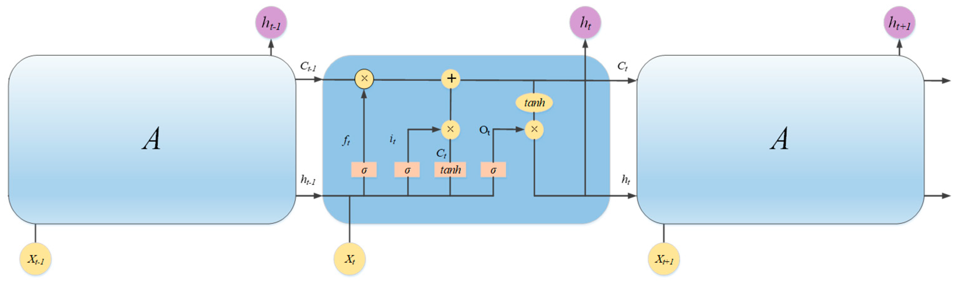
LSTM (Long Short-Term Memory) networks are a special type of Recurrent Neural Network (RNN), with the internal structure shown in Figure 2. The A in figure represents the same neural network module as the intermediate structure. The core component is the memory cell, responsible for storing and transmitting information, and it has the capability of long-term memory. As a deep learning method, LSTM can achieve better approximation of high-dimensional functions by utilizing a large number of training samples, uncovering hidden information within the data, and enhancing modeling capabilities based on multi-layer nonlinear transformations. It also effectively addresses issues such as vanishing and exploding gradients during training. Additionally, LSTM excels at handling time series problems, as it can learn long-term dependencies. Since the power consumption load of each user is inherently a time series, this paper uses an LSTM network for load forecasting.

$$f_t=\sigma (W_f{x}_t+U_f{h}_{t-1}+b_f),$$

(8)

$$i_t=\sigma (W_i{x}_t+U_i{h}_{t-1}+b_i),$$

(9)

$$o_t=\sigma (W_o{x}_t+U_o{h}_{t-1}+b_o),$$

(10)

$${\tilde{C}}_t=\tanh (W_c{x}_t+U_c{h}_{t-1}+b_c),$$

(11)

$$C_t=f_t\odot C_{t-1}+i_t\odot {\tilde{C}}_t,$$

(12)

$$h_t=o_t\odot \tanh (C_t),$$

(13)

Equations (8)–(13) describe the operations of the LSTM unit from a mathematical perspective, where σ and tanh represent the sigmoid and hyperbolic tangent activation functions, respectively. f_t, i_t, and o_t are the sigmoid activation output of the forgetting, input, and output gates, respectively. W_f, W_i, W_c, and W_o are the weight of the input x_t. U_f, U_i, U_o, and U_c are the weight of the previous output; h_t−1, b_f, b_i, b_o, and b_c are the deviation; and $\odot$ indicates Hadamard product.

The LSTM network is particularly well suited for load forecasting due to its ability to capture long-term dependencies in time series data. Unlike standard RNNs, which suffer from vanishing gradient problems when modeling long sequences, LSTM’s gated architecture (comprising input, forget, and output gates) enables selective retention and forgetting of information over extended time horizons. This is crucial for load forecasting, where patterns such as daily and weekly cycles, seasonal variations, and holiday effects must be modeled accurately. Additionally, LSTM’s robustness to noise and its ability to handle irregular time intervals make it an ideal choice for real-world load data, which often contain missing values and anomalies. Compared to other RNN variants like Gated Recurrent Units (GRUs), LSTM provides more explicit control over memory retention, which is particularly beneficial for capturing complex temporal dependencies in electricity consumption patterns.

In this paper, LSTM will be used as the global model for federated deep learning to train the clients. Each responding user is an independent client, and the network topology is shown in Figure 1.

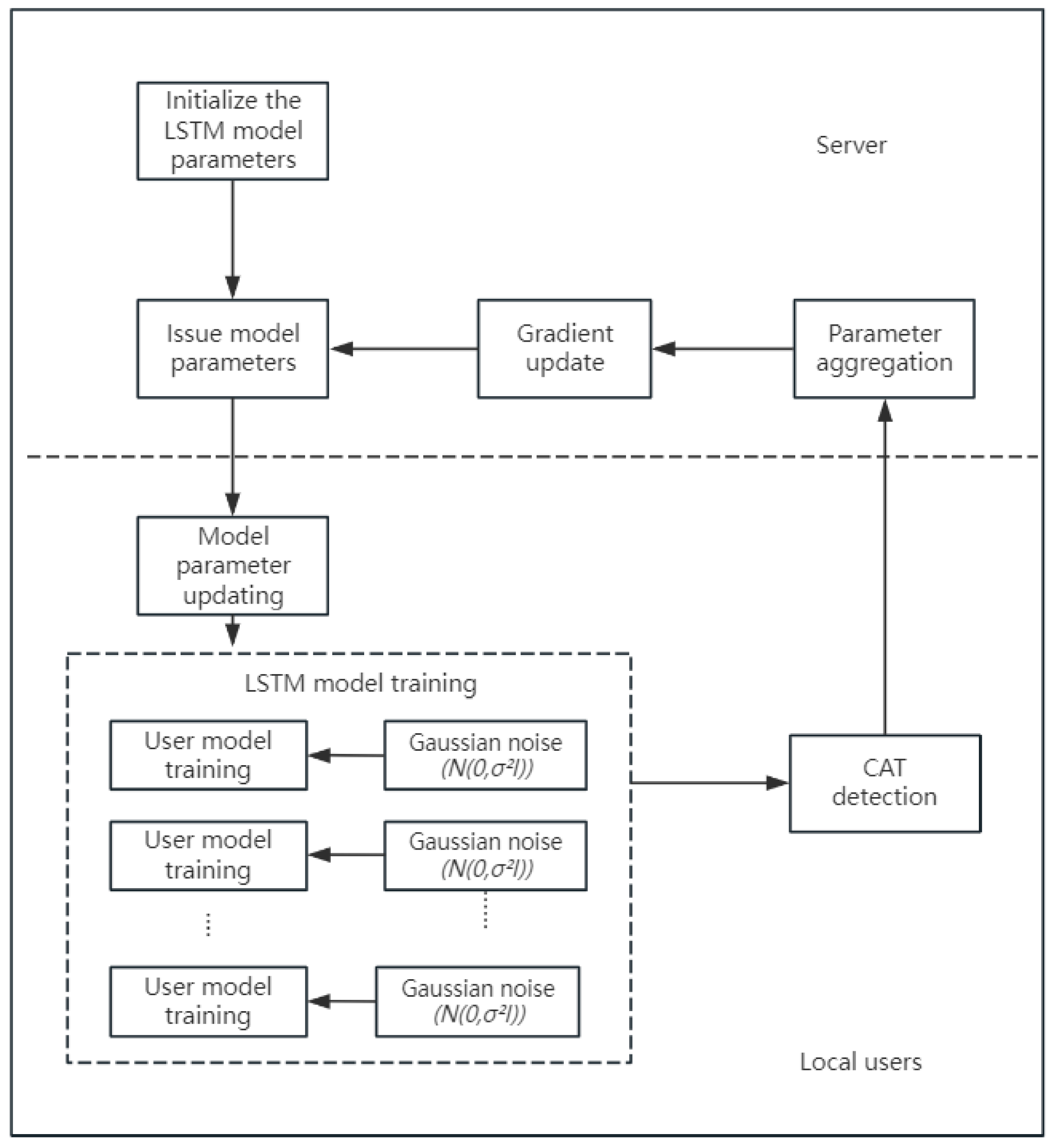
4.3. Differential Privacy Federated Learning Load Forecasting Process

Using Algorithm 1, the power load forecasting process includes the central server initializing the LSTM model parameters and distributing the model parameters, local user data preprocessing, local LSTM model differential privacy training, CAT detection, and if the trigger threshold is met, uploading the LSTM model parameters. The central server then aggregates the parameters and performs global gradient updates, followed by distributing the updated model and starting the next round of training, as shown in Figure 3.

5. Results Analysis

This section validates the effectiveness of the proposed scheme through a case study. The experimental environment is as follows: the CPU is an Intel Core i7-12700K, the GPU is an NVIDIA RTX 3080 Ti 12GB, the memory is 64 GB, the operating system is Ubuntu 21.04, the Pytorch version is 2.0.0, the CUDA version is 11.8, and the Python version is 3.8.16. The deployment mode is single-machine.

5.1. Construction of User Dataset and Data Source

In this paper, weather and time factors are selected as correlated influences on load. The input data feature types include weather, load, and time. Weather factors, such as temperature, humidity, and atmospheric pressure, are used to capture the impact of weather on the load. Time factors, including year, month, day, and hour, reflect the periodicity of the load. The feature selection and transformation process for the dataset is detailed in

Table 1. Feature selection and feature transformation of datasets.

Feature Type	Feature	Type	Unit/Scope	Conversion Mode	Post-Conversion Features
weather	temperature	continuation	°F	normalization	temperature
	Humidity	continuation	%	normalization	humidity
	atmospheric	continuation	kPa	normalization	pressure
load	load	continuation	kW	normalization	load
time	2018 month oh	continuation continuation continuation continuation	2016–2018 1–12 1–30 0–23	One-Hot encoding sin/cos cycle encoding sin/cos cycle encoding sin/cos cycle encoding	oh-2016, oh-2017, oh-2018 month-sin, month-cos day-sin, day-cos hour-sin, hour-cos

.

The experiments utilize the HUE dataset [31], which comprises hourly energy consumption data for residential buildings in British Columbia. This dataset spans nearly three years and includes both energy usage and meteorological data from 22 homes. With a temporal resolution of 24 data points per day, the study focuses on data from 1 June 2016 to 29 January 2018, specifically for homes with IDs 3–14 and 18–20, encompassing 15 users in total. The dataset for each user is partitioned into three subsets, 80% for training, 10% for testing, and 10% for validation, ensuring a robust evaluation of the model’s performance.

5.2. Data Preprocessing

After selecting the appropriate data, preprocessing is required. For missing data, this paper uses either the mean value or interpolation methods to handle it. The specific methods are as follows:

$${\gamma }_i=\left\{\begin{array}{cc}{\displaystyle \frac{{\gamma }_{i-1}+{\gamma }_{i+1}}{2}},& {\gamma }_i\in \mathrm{Null}, {\gamma }_{i-1},{\gamma }_{i+1}\notin \mathrm{Null};\\ 0,& {\gamma }_i\in \mathrm{Null}, {\gamma }_{i-1} \mathrm{or} {\gamma }_{i+1}\in \mathrm{Null},\end{array}\right.$$

(14)

where γ_i is the power load value for a certain time period.

Additionally, to accelerate the convergence speed during model training and improve training efficiency, continuous data values will be normalized as follows:

$${\gamma }_{\mathrm{nom}}={\displaystyle \frac{\gamma -{\gamma }_{\min }}{{\gamma }_{\max }-{\gamma }_{\min }}},$$

(15)

where γ is the original data; γ_nom is the normalized data; and γ_max and γ_min are the maximum and minimum values in the series data, respectively.

5.3. Model Parameters

Choosing appropriate model parameters can effectively accelerate the convergence speed of the model and improve its performance. The setting of LSTM hidden layers mainly includes setting the number of hidden layers and the number of neurons. In this paper, these model parameters are optimized through grid search. A simple load forecasting task is setup to test the performance of the model under different parameter settings and select the optimal parameters based on this. The model parameter settings used for load prediction in this example are shown in

Table 2. Model parameters.

Parameters	Value
Number of epochs of training on clients	8
Total communication rounds	60
LSTM hidden layers	2
Model structure	LSTM layers with 256 hidden states
	LSTM layers with 128 hidden states
	Fully connected layers with 64 neurons
	Fully connected layers with 32 neurons
Input feature dimensions	27
Batch size	128
Learning rate ${\eta }_{\mathrm{g}},{\eta }_l$	0.0015
Dropout probability	0.2
Output feature dimensions	15
Privacy budgetε	0.6
Loss	MSE

.

5.4. Evaluating Indicator

To evaluate the accuracy of the algorithm, three metrics are used to assess the performance in terms of prediction error: Mean Square Error (MSE), Root Mean Square Error (RMSE), and Mean Absolute Percentage Error (MAPE). The specific calculation formulas are given by Equations (16)–(18).

MSE is calculated as follows:

$$MSE={\displaystyle \frac{{\displaystyle {\sum }_{i=1}^N{({\widehat{y}}_i-y_i)}^2}}{N}}.$$

(16)

RMSE is calculated as follows:

$$RMSE=\sqrt{{\displaystyle \frac{{\displaystyle {\sum }_{i=1}^N{({\widehat{y}}_i-y_i)}^2}}{N}}}.$$

(17)

MAPE is calculated as follows:

$$MAPE={\displaystyle \frac{1}{N}}{\displaystyle {\sum }_{i=1}^N\frac{\left|{\widehat{y}}_i-y_i\right|}{y_i}}\ast 100\%.$$

(18)

where N is the number of test samples, and ${\widehat{y}}_i$ and $y_i$ are the actual and predicted reads in kWh, respectively.

5.5. Current Mainstream Algorithms Involved in Comparison

(1)

FedAvg: Standard Federated Averaging algorithm.

(2)

FedAdaGrad: Federated Adaptive Gradient algorithm.

(3)

DCScaffold: The algorithm proposed in this paper.

To comprehensively evaluate the performance of the proposed DCScaffold algorithm, we compare it with two current mainstream federated learning algorithms: FedAvg and FedAdaGrad. FedAvg, as the foundational algorithm in federated learning, serves as a standard benchmark for communication efficiency and model aggregation. FedAdaGrad, on the other hand, addresses non-IID data challenges through adaptive optimization techniques, making it a representative method for handling data heterogeneity. By comparing DCScaffold with these widely adopted approaches, we aim to highlight its advancements in simultaneously addressing communication efficiency, privacy preservation, and non-IID data handling. This comparative analysis provides a clear understanding of the strengths and limitations of each algorithm in the context of load forecasting.

5.6. Analysis of Simulation Result

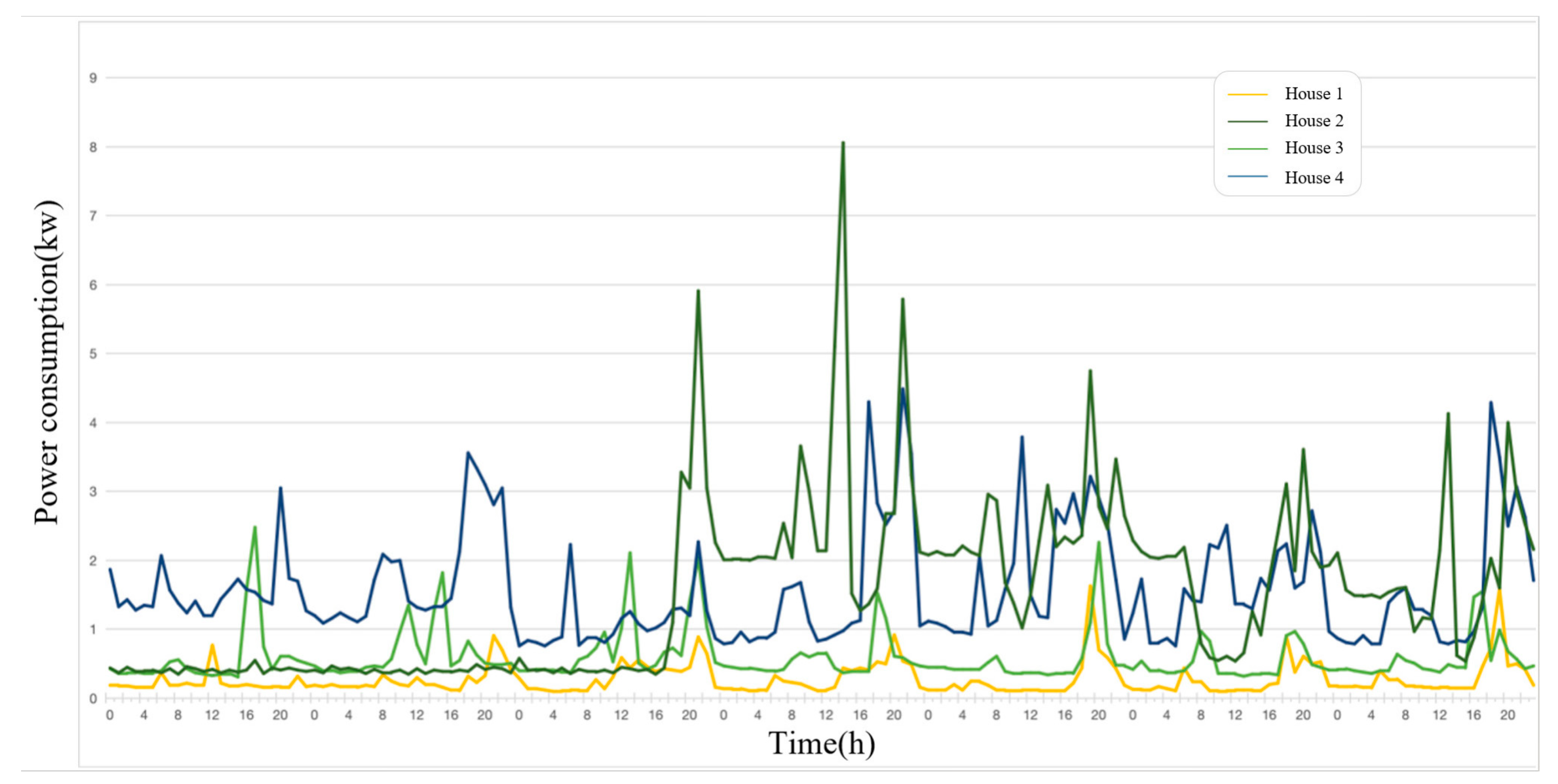
Figure 4 shows the power load changes in the four randomly selected users during the week from 1 September 2017 to 7 September 2017. By comparing the power load curve, it can be observed that different power behaviors occur between different users.

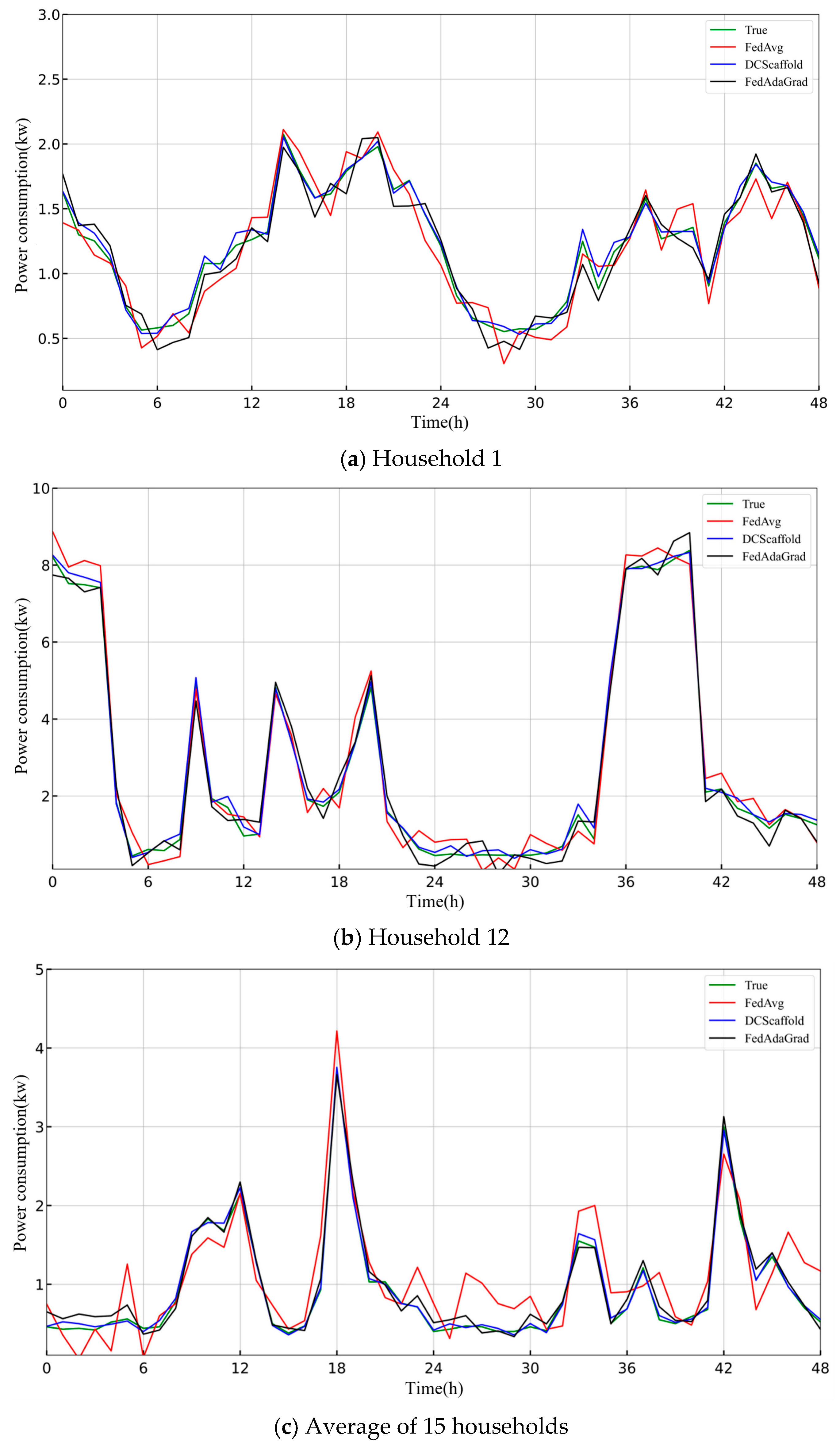
Figure 5 compares the prediction results of three federated learning algorithms: FedAvg, DCScaffold, and FedAdaGrad. Whether for a single user’s highly fluctuating load (e.g., User 1) or the relatively smoother load curve averaged across multiple users, the DCScaffold algorithm demonstrates the highest prediction accuracy. Its predicted curve most closely matches the actual values, especially excelling in fitting complex and highly fluctuating patterns. This confirms that the algorithm effectively overcomes the negative impacts of heterogeneous data by introducing an adaptive correction mechanism. Although the prediction quality of the FedAdaGrad algorithm is better than the classic Federated Averaging algorithm, it still exhibits some bias at peak points, with overall performance falling between the other two algorithms. FedAvg, however, fails to adequately address non-IID data, and its prediction results show the largest discrepancy from the actual values, with noticeable over- or under-estimations at several time points. The experimental results demonstrate the significant advantages of the improved DCScaffold algorithm over the classic algorithms when dealing with data heterogeneity.

Table 3. Comparison of different algorithms in MSE, RMSE, and MAPE.

Algorithm	MSE	RMSE	MAPE
FedAvg	0.131	0.362	22.9
FedAdaGrad	0.032	0.178	13.8
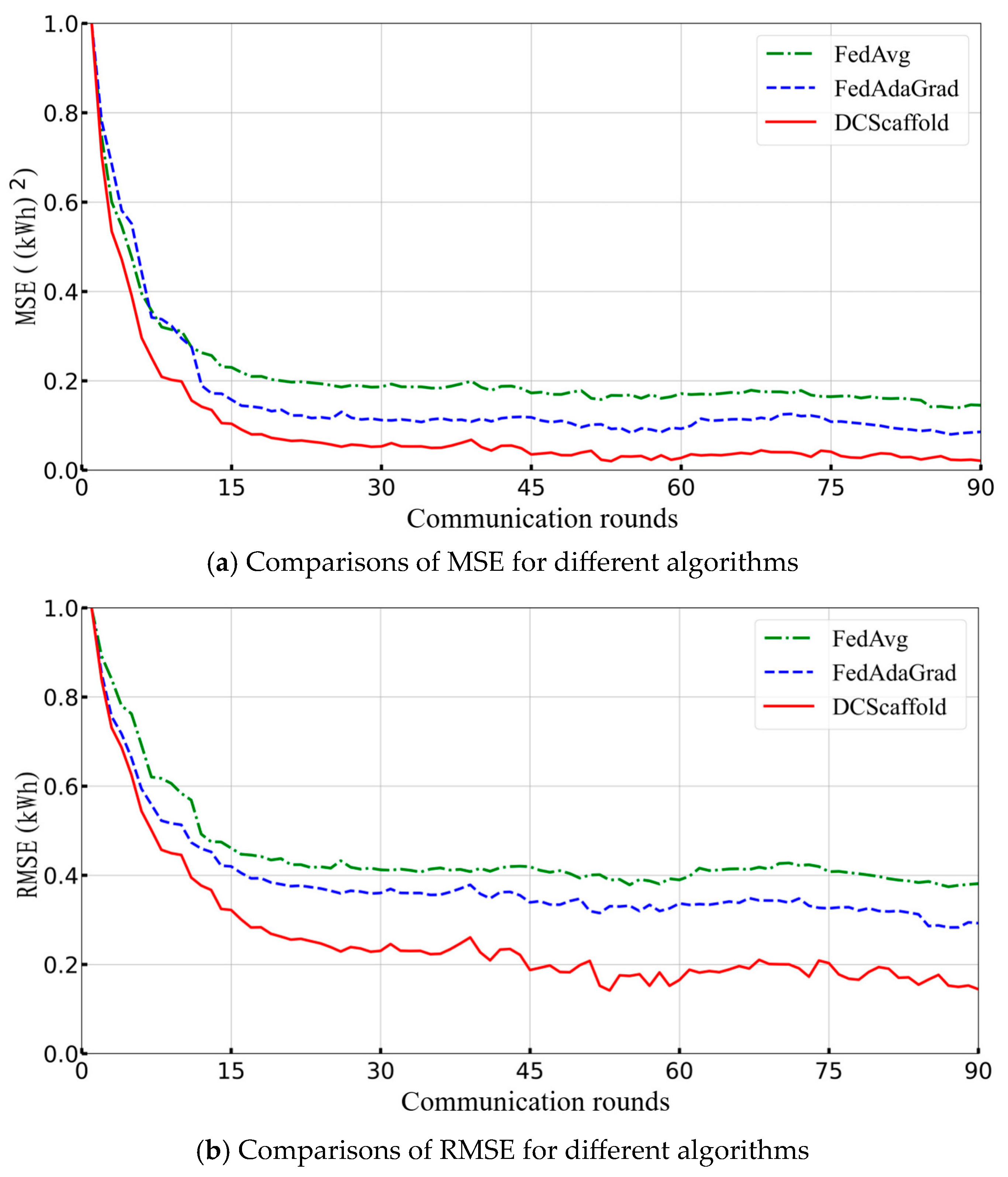
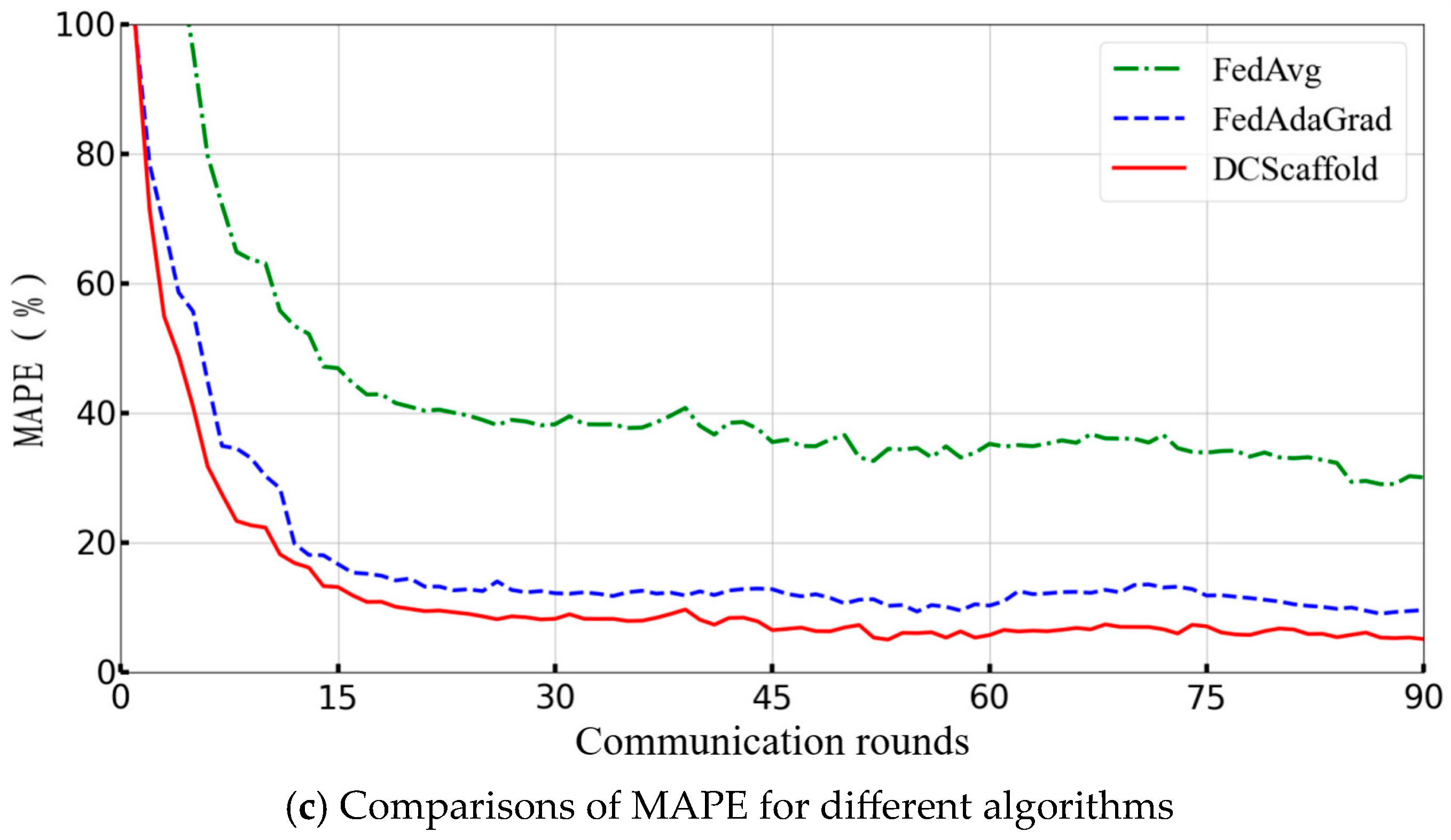
DCScaffold	0.019	0.138	9.47

and Figure 6 provide a comparative analysis of the three federated learning algorithms (FedAvg, DCScaffold, and FedAdaGrad) across three evaluation metrics: MSE, RMSE, and MAPE. Whether considering Mean Square Error (MSE), Root Mean Square Error (RMSE), or Mean Absolute Percentage Error (MAPE), the DCScaffold algorithm consistently achieves the best performance across all metrics, demonstrating the highest prediction accuracy and robustness when handling heterogeneous data. We know that the smaller the privacy budget setting in DP, the better the privacy protection, and the worse the prediction accuracy. Due to the introduction of random noise, the DP noise degrades model performance. Through comparison, under the privacy budget 0.6, the proposed algorithm can achieve better prediction performance than the current mainstream federated learning algorithms. Comparison with a traditional DP strategy suggests that our approach significantly mitigates the negative effects of DP on the model. FedAvg still struggles to effectively address the data heterogeneity issue, with the poorest performance in all three metrics. Although the adaptive FedAdaGrad algorithm outperforms FedAvg in all metrics, there is still room for improvement, and its overall performance lies between the other two algorithms. These evaluation results are fully consistent with the earlier analysis of the algorithm’s prediction curves, further validating the significant advantage of the DCScaffold algorithm over classical algorithms when dealing with data heterogeneity.

Table 4. Comparison between FedAvg and CAT approach.

Method	MSE	RMSE	MAPE	Save Communication
FedAvg	0.14	0.37	22.9	0
CAT1	0.019	0.138	9.4	16.2%
CAT2	0.19	0.43	28.3	78.9%
CAT3	0.23	0.48	31.5	83.3%
CAT4	0.45	0.67	45.3	89.7%

provides a comparison between FedAvg and the CAT method, showing results for four different scenarios: CAT1 with a threshold of 0.1%, CAT2 with a threshold of 2%, CAT3 with a threshold of 4%, and CAT4 with a threshold of 10%. Figure 7a–c compares the performance of the FedAvg algorithm and the CAT method in terms of MSE, RMSE, and MAPE. The results show that the performance of the CAT1 algorithm is the best, significantly outperforming the FedAvg algorithm while saving 16.2% of communication overhead. Since CAT1 has a lower threshold, it achieves good model performance but with limited communication savings. The performance of the CAT2 algorithm is slightly lower than FedAvg, but it saves nearly 80% of the communication overhead, making it highly practical for models with large global model sizes and many clients. Additionally, from Figure 7 and Table 4, it can be observed that the higher the CAT threshold, the more communication is saved, but the global model performance decreases. CAT4 can save almost 90% of the communication overhead, and using the CAT method achieves a savings of about 80% in communication overhead while reaching the preset accuracy, effectively balancing communication bandwidth and model performance.

6. Conclusions

This study proposes a novel differential privacy federated learning algorithm, DCScaffold, which integrates differential privacy mechanisms, CAT strategy, and adaptive correction terms into the SCAFFOLD framework. By addressing the challenges of communication efficiency, privacy preservation, and non-IID data handling simultaneously, DCScaffold demonstrates significant improvements over existing methodologies. Experimental results on real-world load forecasting data show that DCScaffold achieves a 48.6% reduction in MSE compared to FedAvg and a 40.6% reduction compared to FedAdaGrad, while saving up to 78.9% of communication overhead through the CAT strategy. Furthermore, rigorous privacy analysis proves that DCScaffold satisfies $(\epsilon ,\delta )$ differential privacy with tighter composition bounds, ensuring robust privacy guarantees. These findings highlight the effectiveness of DCScaffold in enhancing prediction accuracy, communication efficiency, and privacy protection for smart grid load forecasting. Future research can focus on other cyber security problems, optimizing algorithms of federated learning, the trade-off between model accuracy and privacy preservation.