Abstract
This document explores short-term hydrothermal economic dispatch (HTED) while explicitly modeling the valve-point effect of thermal units as a factor that adds complexity to power system optimization. Two nature-inspired optimizers, the Bat Algorithm (BAT) and the Artificial Bee Colony (ABC) algorithm, were used on a 24 h horizon for nine unit power plants (five thermal, four hydro). After 30 independent runs, BAT produced the lowest daily operating cost at USD 307,952.44, whereas ABC obtained USD 311,457.48, a 1.14% saving (USD 3.5 k) in favour of BAT. However, ABC converged almost twice as fast, stabilizing after around 40 iterations, while BAT required around 80 iterations. The results demonstrate that BAT offers a modest but measurable economic advantage, whereas ABC provides faster convergence, which is important when real-time computational limits dominate. These quantitative findings confirm that meta-heuristic techniques are practical tools for HTED and highlight the trade-off between cost minimization and computational speed.
1. Introduction
In an electrical power system, one expects to find different generation units (depending on the energy source); some of these types are hydroelectric, thermal, wind, and solar, among others. Some countries have primarily hydroelectric and thermal generation plants to meet the electricity demand of the entire country, which is why electrical operators must, as a priority, find better technical and computational solutions for hydrothermal economic dispatch [1].
Economic dispatch is one of the most essential optimization problems for the electricity sector [2,3], since it aims to determine the power produced by each generation unit involved in supplying the demand by guaranteeing the electricity supply at minimum cost [4,5].
Being an optimization problem, the economic dispatch minimizes an objective function that is related to the operating costs of the generation plants (fuel cost, depreciation expenses, maintenance cost, etc.) [6,7]. On the other hand, to have a safe operation of the electrical system and thus be able to supply the demand without any novelty, a set of technical (losses of the operating system) and operational (power balance) restrictions must be included [5].
In the literature, several works have addressed hydrothermal dispatch, using mathematical methods to graphic methods [8,9]. In [10], a program for short-term economic dispatch is developed using the artificial bee colony algorithm. In this article, fuel costs are reduced in thermal power plants, and in parallel, the maximum cost–benefit of hydroelectric power plants is achieved.
In [11], the solution of the economic dispatch problem of thermal power plants, hydroelectric power plants, and wind power plants is proposed using the double-weighted particle swarm algorithm.
In [12], a fast time-variable acceleration coefficient particle swarm optimization algorithm is proposed to solve economic emission dispatch problems consisting of the combined economic emission dispatch of heat and power, taking into account operational constraints (boundaries) such as ramp rate, valve point effect, the impact of power transmission loss, rotary reserve requirements, and prohibited operating zones.
In [2], the optimum dynamic generation dispatch solution is presented considering a multi-objective criterion and valve point effect through MATLAB’s Genetic Algorithm optimization tool. The objective of the article is to find the active power from power plants for a given time, such that it allows minimizing the cost of generation and the emissions of polluting gases while satisfying all the restrictions of equality and inequality (speed limits of active power generation ramps and the effect of valve points). Also, on issues of pollution reduction, in [3], a low-carbon economic dispatch model is developed by incorporating the emission penalty scheme, in which the cost related to the penalty is considered part of the objective function.
In [13], a mathematical optimization algorithm is developed and proposed for the optimal operation focused on the economic dispatch for DC microgrids with high penetration of distributed generators and energy storage systems through semi-defined programming that allows transforming the non-linear characteristics and non-convex parts of the economic dispatch problem into a convex approximation.
In [14], a dynamic programming-based algorithm is developed to solve the hydrothermal economic dispatch problem. This algorithm allows the dispatch of the combined generation of both thermal and hydroelectric power plants, including the hydraulic coupling.
By considering all of the factors above, it is possible to understand the issues surrounding economic dispatch in systems with hydroelectric and thermoelectric components. The mathematical formulation entails the same considered variables and operational restrictions, such as water flows, storage systems (reservoirs), and the effect of the point valve, among others; as a consequence, computational problems may exist when finding the optimal results [15,16].
Consequently, the hydrothermal economic dispatch problem—non-linear, non-convex, and NP-hard owing to the valve-point effect, reservoir coupling, and multiple equality/inequality constraints—becomes an ideal candidate for heuristic and meta-heuristic optimization. Such methods do not rely on gradient information, tolerate discrete decision variables, and deliver high-quality solutions within the strict time windows required by modern energy-management systems. Among the many available meta-heuristics, the Bat Algorithm (BAT) and the Artificial Bee Colony (ABC) stand out for their small number of control parameters, proven robustness on non-convex cost functions, and complementary search philosophies. BAT emphasizes exploitation through frequency-modulated echolocation. In contrast, ABC offers strong exploration via adaptive neighbor search. Accordingly, the present work applies BAT and ABC to the short-term hydrothermal dispatch with valve-point effect, evaluating their performance to illustrate the practical trade-off between economic savings and computational speed.
Several studies have already demonstrated that both BAT and the ABC can be adapted to hydrothermal optimization. For example, a real-time BAT variant lowers operating cost by 1.7% while coping with minute-to-minute renewable fluctuations [17], and a multi-objective BAT that jointly minimizes fuel cost and emissions across four interconnected areas consistently outperforms PSO [18]. On the ABC side, an adaptive ABC accelerates long-term cascade scheduling by dynamically adjusting modification rates [19], whereas an enhanced ABC tailored to fixed-head dispatch achieves both a lower fuel cost and shorter run-time than differential evolution and evolutionary programming [20]. For short-term horizons, a multi-objective ABC with progressive-optimality local search yields a superior Pareto front to NSGA-II and MODE [21], and even a well-tuned standard ABC can produce the minimum daily cost when transmission losses are considered [10].
These contributions confirm that BAT and ABC are flexible and efficient tools for hydrothermal dispatch; however, none of them incorporates the valve-point effect, a ripple term that makes the cost function highly non-convex and closer to real thermal unit behavior. The present work fills this gap by extending the hydrothermal formulation to include valve-point ripples and by applying both BAT and ABC to solve the problem.
This article presents the following sections: In Section 2, a bibliographical review is carried out regarding formulating the economic dispatch with all the technical and operational restrictions considered in the study. For this, emphasis is placed on studying the BAT and ABC algorithms. The ant colony algorithm theoretically delivers a better result in terms of optimization. Thus, it will go hand in hand with the theory to effectively verify which method is better. In Section 3, two algorithms based on heuristic techniques are developed and formulated to solve problems of systems with hydroelectric and thermoelectric power plants. Section 4 presents case studies and analyzes results obtained using a test system of nine generators. Finally, in Section 5, the conclusions of the research are presented.
2. Hydrothermal Economic Dispatch
2.1. Hydroelectric Generation Plants
Hydroelectric power plants use the hydraulic energy of the water flow (position, speed, or both). A typical hydroelectric plant is shown in Figure 1. Hydroelectric power plants have numerous advantages compared to fossil fuel power plants and plants with other renewable sources. Regarding fossil sources, they have the advantage of reducing pollution, mainly CO2 emissions, which are the leading cause of the greenhouse effect. Water’s density is much greater than that of air or wind; therefore, if the swept area is equal, the energy obtained from water is more significant than that from wind of the same speed. Hydroelectric power generation is considered one of the cheapest in terms of cost per kWh (marking a reduction in generation operating costs since this technology is not subject to the costs of fossil fuels). For this reason, hydroelectric power is the first investment option for companies. These power plants are highly reliable and can quickly respond to changes in demand for electricity, making them the most dependable source of energy [22,23,24].
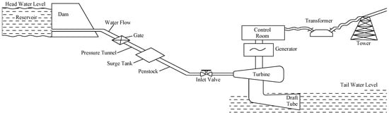
Figure 1.
Typical hydroelectric power plant.
2.2. Thermal Generation Plants
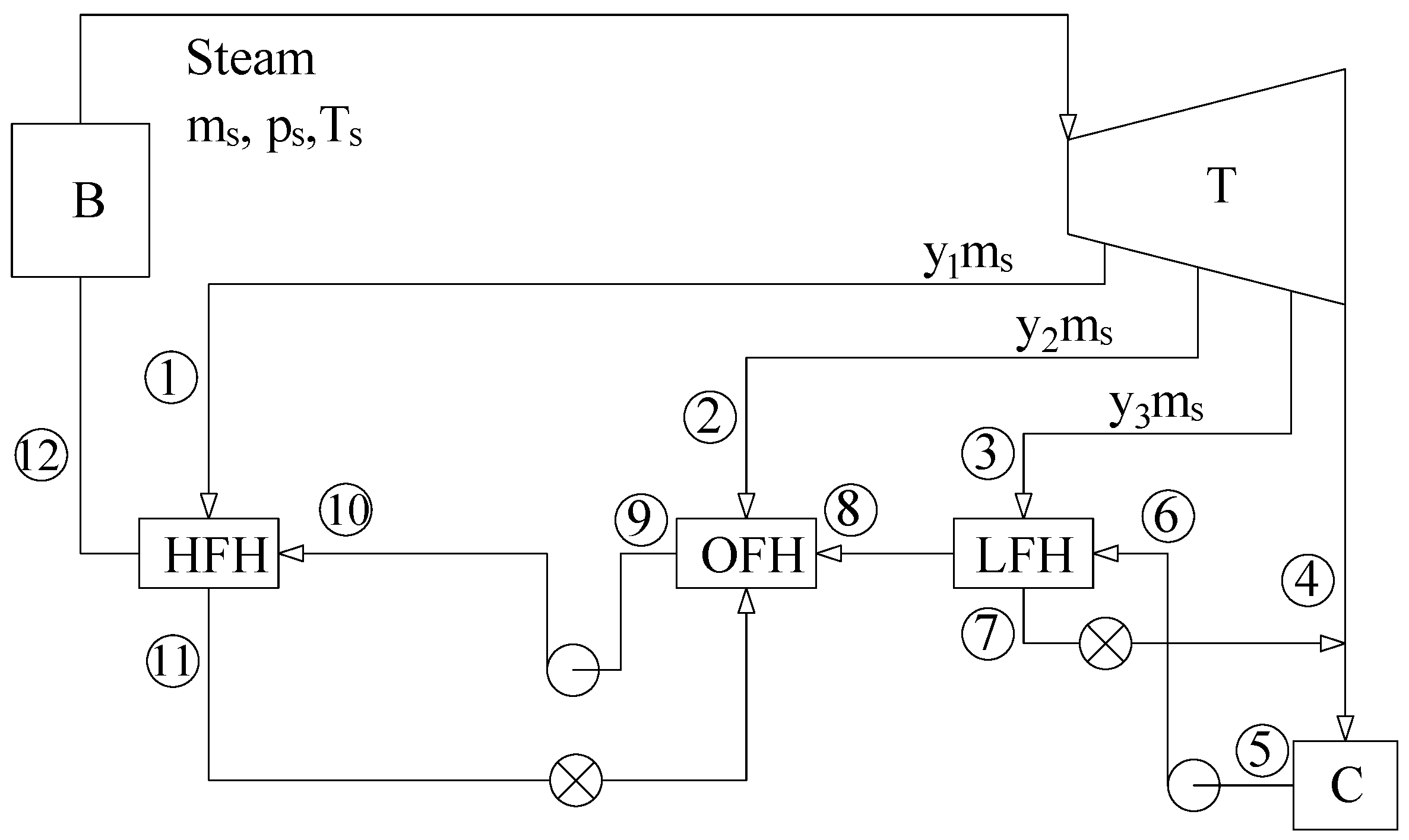
Fossil fuels are the primary fuel for thermal power plants, but there is a fear that they will eventually run out over time, which is why plants with renewable energy sources (water, solar, wind, etc.) are used. However, for large systems, renewable sources are not as efficient as the only energy sources due to the uncertainty of their variables (air, water flow, and solar radiation). Therefore, it is used as a backup power source in conjunction with a thermal power plant by partial load sharing. A typical steam thermal power plant is shown in Figure 2, consisting of a boiler (B), a steam turbine (T), a condenser (C), three feedwater heaters, and two pumps [25,26].
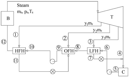
Figure 2.
Typical thermal power plant.
2.3. Short-Term Hydrothermal Economic Dispatch
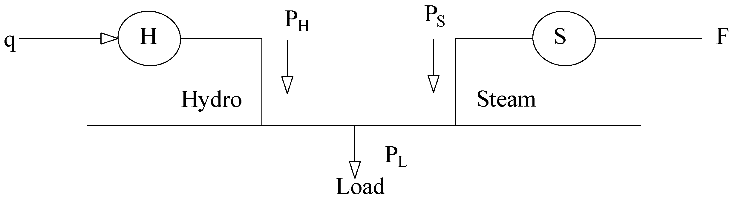
The short-term hydrothermal economic dispatch (HTED) (Figure 3) in electrical power systems is carried out from a daily horizon to a weekly horizon. The main objective of the problem is to minimize the operating cost of thermal units by optimizing the use of the available water, thus satisfying the load demands of the system without violating its constraints [27,28,29].
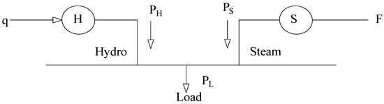
Figure 3.
Hydrothermal economic dispatch.
Next, the formulation of the HTED problem is presented together with the technical and economic constraints applied to an electrical power system.
2.3.1. Objective Function
The production costs of hydroelectric plants are considered insignificant because the water resource is used directly from nature for free; the objective function for the HTED depends exclusively on the fuel cost of the thermal power plants [27,28], and is represented using a second-degree polynomial equation, as described below, in Equation (1). Also, in line with recent studies, the variable operating cost of hydropower is commonly neglected because “the operating costs of thermal power plants are mainly fuel costs, while hydropower plants … do not need to be paid” [30].
where
- F is the fuel cost function of the i-th thermal power unit during interval m [USD/h].
- is the power generated by the i-th thermal power unit during interval m [MW].
- [USD/h] is the fixed (no–load) cost coefficient.
- [USD/(MWh)] is the linear fuel–cost coefficient.
- [USD/(MW2h)] is the quadratic fuel–cost coefficient.
- t is the total number of operating periods.
- N is the total number of thermal plants.
It is important to consider that in thermal power plants, steam flow to each turbine is regulated by a set of valves. To optimize efficiency, these valves open sequentially based on power demand. This sequential operation introduces a nonlinearity in the fuel cost function, commonly referred to as the valve point effect.
A sinusoidal function represents the valve point effect and makes the quadratic function formulated in Equation (1) become a new cost function of the non-uniform and non-differentiable type [27,29]. The cost of production for thermal power plants changes due to the valve point effect. The new objective function is a sum of a quadratic and sinusoidal function, as shown in Equation (2).
where
- represents the minimum generation power of each plant.
- [USD/h] is the amplitude of the valve-point ripple in the fuel–cost curve.
- [rad/MW] is the ripple frequency factor.
2.3.2. Equality Constraints
The power balance is one of the restrictions that must be respected when formulating the economic dispatch problem. This restriction is defined in the following expression:
where
- , represent the power delivered, respectively, by the thermal and hydroelectric power plants during the time interval m.
- M is the number of hydroelectric power plants.
The parameter represents the load demand and describes power losses in the transmission system for each time interval in the planning horizon.
In Equation (3), the losses that occur in the lines of the electrical power system due to Joule’s effect are directly considered. The total losses in the transmission system can be quantified through Equation (4).
where
- , , are the coefficients of the system loss matrix.
Another equal constraint is related to the delivered power by a hydroelectric plant. It can be represented as a quadratic function that depends on the amount of water released to the turbines and the volume of its reservoir, as indicated below in Equation (5), which is a non-convex and non-uniform constraint [8].
where
- represents the expected storage volume at the end of the time interval t.
- refers to the amount of water that passes through a turbine within a specific period t of the planning horizon.
- is the head-dependent power term proportional to the square of the forebay storage volume .
- is the turbulent loss term proportional to the square of turbine discharge .
- interaction term that couples available head and discharge ().
- and are the linear contributions of storage volume and discharge.
- is the constant offset representing the no-load output when the unit is synchronized.
Additional constraints related to reservoir volumes include the initial water elevation level (6), which defines the starting condition of each hydroelectric plant at the beginning of time interval, and the final elevation level (7), which must be ensured at the end of the last time interval within the 24-h planning horizon.
Finally, the constraint related to the dynamic balance of the water in the reservoirs is formulated in Equation (8) and completes the hydraulic generation to address the hydrothermal dispatch problem.
where
- is the storage volume of the reservoir of the hydroelectric unit in the time interval t − 1.
- is the natural net inflow for each hydroelectric plant in the interval t.
- is the spill rate during the interval t.
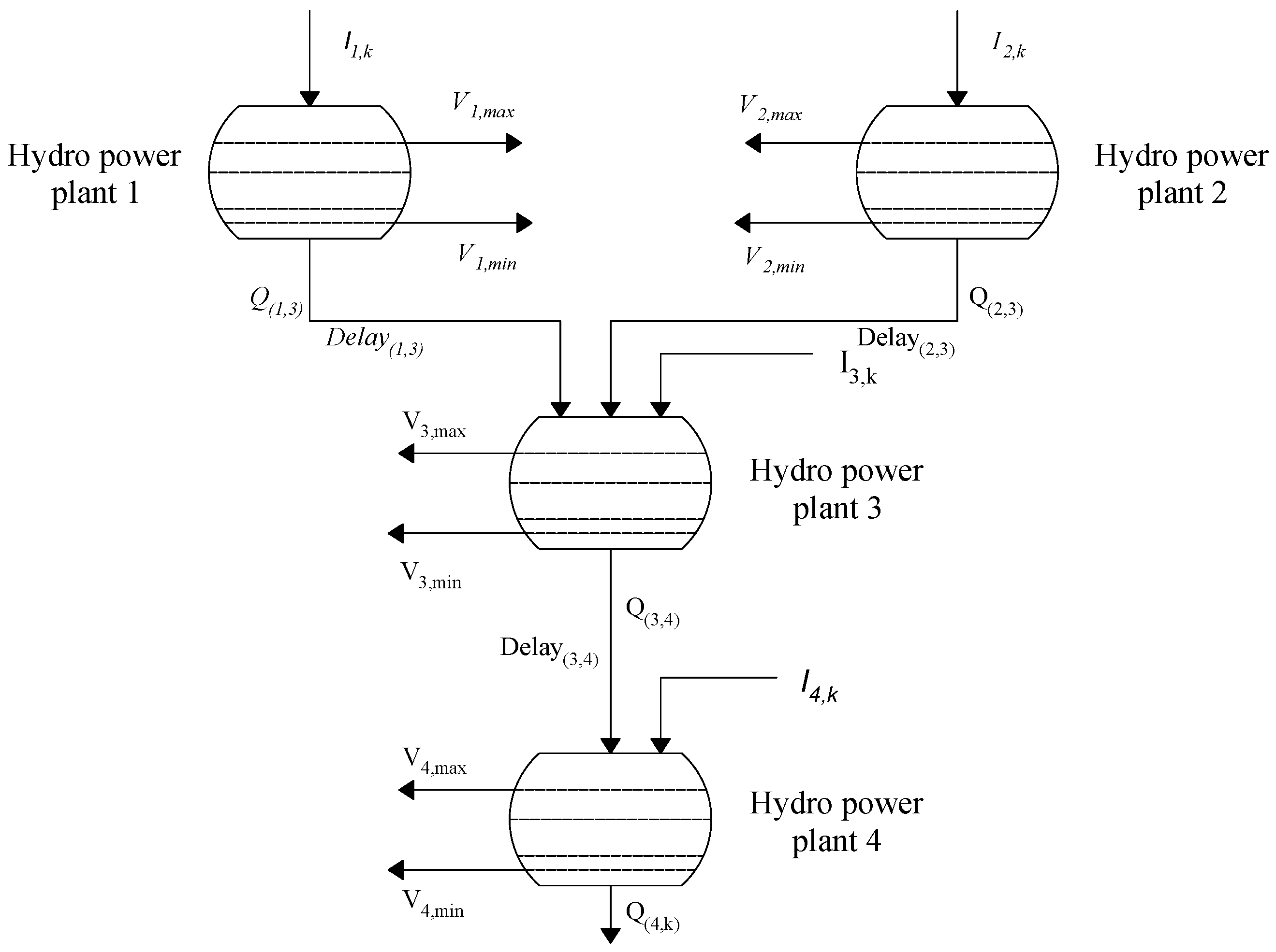
Equation (8) can present a variation when considering the hydraulic coupling between hydroelectric power plants, as illustrated in Figure 4, which implies that the volume of the reservoir of a given power plant downstream in a time interval also considers the turbine flow and the spillage rate of the plants that are immediately upstream of it. The modification of the hydraulic continuity equation is detailed in Equation (9).
where
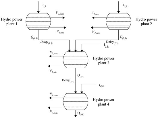
Figure 4.
Cascade model of hydropower plants.
- , represent the water discharges and spills coming from the hydroelectric plants that are directly above plant j
2.3.3. Inequality Constraints
The output power limits of hydroelectric and thermal power plants are a type of constraint that helps define the search space, which must be followed to determine the dispatch scheme that offers the lowest cost for the proposed objective function.
Equations (10) and (11) refer to the minimum and maximum generation power capacity in which thermoelectric and hydroelectric plants must operate, respectively.
Hydroelectric generation power depends on the reservoir storage volume and turbine flow rate. Equations (12) and (13) determine the minimum and maximum physical limitations that must be considered concerning the storage capacity of the reservoirs and the flows of water discharges that can pass through the hydraulic turbines.
3. Methodology
The proposed approach uses two optimization methods as essential tools for conducting research. These methods were chosen for this research since they have successfully solved problems like hydrothermal dispatch while being adjusted specifically for this study’s distinct features, which included the valve point effect and hydroelectric reservoir constraints.
3.1. Bat Optimization Algorithm
The Bat Optimization Algorithm (BAT) is a metaheuristic optimization algorithm that emulates the echolocation behavior of bats. It was proposed by Xin-She Yang in 2010 as an extension of the standard Bat Algorithm. The BAT is designed to solve optimization problems by mimicking the behavior of bats searching for prey [31]. Here is a general overview of how BAT works:
- Initialization: The algorithm initializes a population of bats, so each bat is shown as a binary string or vector encoding a possible solution to the optimization problem.
- Echolocation: In the echolocation phase, each bat emits pulses or calls to explore the search space. The frequency and loudness of the pulses determine the bat’s position and loudness, respectively. The loudness of a bat is typically associated with the quality or fitness of its solution.
- Movement: Based on the emitted impulses, each bat adjusts its position in the search space. The new position is established by incorporating a random walk into the current position of the bat, which is influenced by the best solution detected so far and the average position of the population.
- Pulse rate and loudness: The pulse rate of each bat is updated to control the loudness of its pulses. Bats with better solutions tend to have higher pulse rates and loudness values.
- Local search: Occasionally, a random bat may perform a local search around its current position to explore the neighborhood more intensively. This helps refine the solutions and escape local optima.
- Updating the best solution: The algorithm keeps track of the best solution found during the search process.
- Termination: The algorithm terminates when a stopping criterion is met, such as reaching a maximum number of iterations or achieving a desired level of solution quality [32,33].
The BAT’s key characteristics include its randomness, the exploitation of reasonable solutions through the pulse rates and loudness of bats, and the exploration of the search space through random walks. These characteristics enable the BAT to effectively search for optimal or near-optimal solutions in various optimization problems. The BAT offers several advantages that make it a popular choice for solving optimization problems.
Exploration and Exploitation Balance: The BAT strikes a good balance between exploration (searching the solution space broadly) and exploitation (refining solutions in promising regions). The echolocation and movement mechanisms of bats in the algorithm allow for global and local search, increasing the likelihood of finding the global optimum.
Flexibility and Simplicity: The BAT is a flexible algorithm that can be easily implemented and adapted to different optimization problems. It does not rely on any specific problem structure or assumptions, making it applicable to many real-world and complex optimization scenarios.
Parallel Search: The BAT is well suited for similar computing environments. The independent nature of bat movements allows for the concurrent evaluation of multiple bat positions, enabling the efficient use of parallel processing capabilities and reducing the overall computation time.
Robustness: The BAT has shown robustness in dealing with noisy or uncertain objective functions. The algorithm’s stochastic nature, randomization in bat movements, and ability to explore different regions of the search space make it less likely to get stuck in local optima.
Fewer Control Parameters: The BAT has a small number of control parameters compared to some other optimization algorithms. This simplifies parameter tuning and reduces the effort required to fine-tune the algorithm for different problems.
High Convergence Speed: The BAT has demonstrated competitive convergence speed in many optimization problems. The combination of adaptive frequency adjustment, velocity updates, and local search mechanisms allows efficient convergence toward the global optimum.
Versatility: The BAT has been successfully applied to optimization problems, including continuous, discrete, and mixed-variable problems. It has been used in engineering design, data mining, image processing, and machine learning, showcasing its versatility.
It is worth noting that the performance of the BAT can depend on factors such as the specific problem being solved, the parameter settings, and the quality of the fitness landscape. It is always recommended to fine-tune the algorithm and compare it with other approaches to ensure optimal performance for a given problem [33,34]. The algorithm implemented for the solution using BAT is presented below in Table 1.

Table 1.
BAT procedure used in this study.
3.2. Artificial Bee Colony Algorithm
The Artificial Bee Colony Algorithm (ABC) is a swarm intelligence optimization technique that mimics the foraging behavior of honey bee colonies. The algorithm was proposed by Dervis Karabogaz in 2005. Like other metaheuristic algorithms, ABC solves optimization problems, especially in continuous search spaces.
The inspiration for this algorithm came from the study of foraging, which refers to animals collecting organic matter from nature and the behavior of bee colonies. Scientists have developed an algorithm called ABC, which is based on the foraging process of bees. In nature, bee colonies start foraging for food when they are hungry. During this process, there are four key elements: the honey source, the leader bee, the follower bee, and the scout bee. These elements work together to produce intelligent behavior in the colony [35,36].
During the foraging process, the queen bee looks out for sources of nectar that are of higher quality and closer in proximity, which are easier to obtain. Lower-quality sources are disregarded. Once the leader bee spots a good nectar source, she passes on the information to other bees. The other bees, who are also known as worker bees, then search for a nearby nectar source. If the worker bees discover a high-quality nectar source, their role changes to that of the queen bee, and they repeat the same process as before. Here is a general overview of the Artificial Bee Colony Algorithm:
- Initialization: Create an initial population of artificial bees (candidate solutions) at random within the search space and subsequently evaluate the fitness (objective function value) of each bee’s position.
- Employed Bee Phase: Each bee searches for a new solution in the vicinity of its current position by adjusting the position according to a specific variation operator (e.g., random search, local search, etc.). Evaluate the fitness of the new solutions and compare them with the previous positions. If the fitness of the new solution is more optimal, the position of the bee is updated; otherwise, it keeps the current position.
- Onlooker Bee Phase: The observer bees analyze the solutions of the employed bees and choose a solution with a probability proportional to its fitness value. The observer bees use the selected solutions as sources of information to perform local searches and generate new candidate solutions.
- Scout Bee Phase: If an employed bee’s solution remains unchanged for a certain number of iterations (cycles), the bee becomes a scout bee. Scout bees abandon their current solutions and randomly generate new solutions within the search space.
- Update Best Solution: Once a cycle is completed, it updates the most optimal solution (the best overall solution) based on the current population of bees employed.
- Termination: Repeat the employed bee, observer bee, and scout bee phases until a termination criterion is met, such as finding a satisfactory solution or reaching a maximum number of iterations.
The ABC’s key parameter is the number of cycles, which controls the exploration and exploitation trade-off. By adjusting this parameter, the algorithm can adapt to different problem complexities and convergence requirements. The ABC is a versatile optimization tool that has been used for various optimization problems ranging from function optimization to engineering design and parameter tuning in machine learning models. It is well known for its simplicity and ability to find near-optimal solutions, even in complex and multimodal search spaces. However, like other metaheuristic algorithms, the performance of ABC may vary depending on the characteristics of the problem and the parameter settings. Therefore, to achieve the best results for a specific problem, it is essential to carefully tune and experiment with the algorithm [10].
The search for nectar by bees is an optimization process. This behavior was modeled as an optimization heuristic based on the biological model, consisting of several elements. This process is presented in Figure 5. Also, the algorithm implemented for the solution using ABC is presented in Table 2.
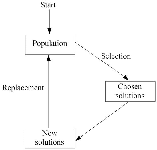
Figure 5.
ABC’s process.
Table 2.
ABC procedure used in this study.
- Food source: The value of a food source depends on several factors, such as proximity to the hive, amount, richness, or concentration of energy, and ease of extraction. As far as the project is concerned, the food source would be considered as the energy to be supplied by each of the generators.
- Forager bees employed: They carry information about that particular source, its distance, location, and profitability to share it with the observing bees.
The exchange of information between bees is essential for the construction of collective knowledge. Through this interaction, the bees will decide the behavior that the hive should carry out.
The control parameters of the two methods were kept constant throughout all experiments to ensure a fair and reproducible comparison. Table 3 summarizes the full setting—population size, stopping criteria, and algorithm-specific coefficients—directly extracted from the MATLAB scripts used in this study.
Table 3.
Parameter settings used for the ABC and BAT algorithms.
4. Results
In this section, we present and discuss the results obtained from applying the two implemented optimization algorithms: the Artificial Bee Colony and Bat Optimization algorithms. The performance of each approach is analyzed in terms of solution quality, highlighting the strengths and limitations observed during the experimentation process.
To test the BAT and ABC algorithms, a demand scenario is proposed, as illustrated in Figure 6, where a 24 h planning horizon is considered.
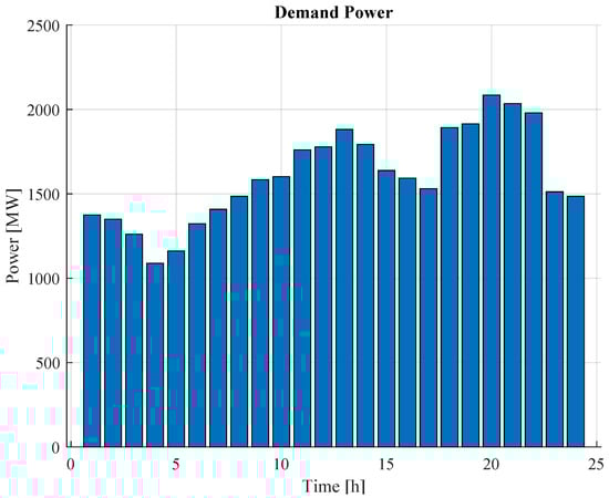
Figure 6.
Planning for a 24 h demand scenario.
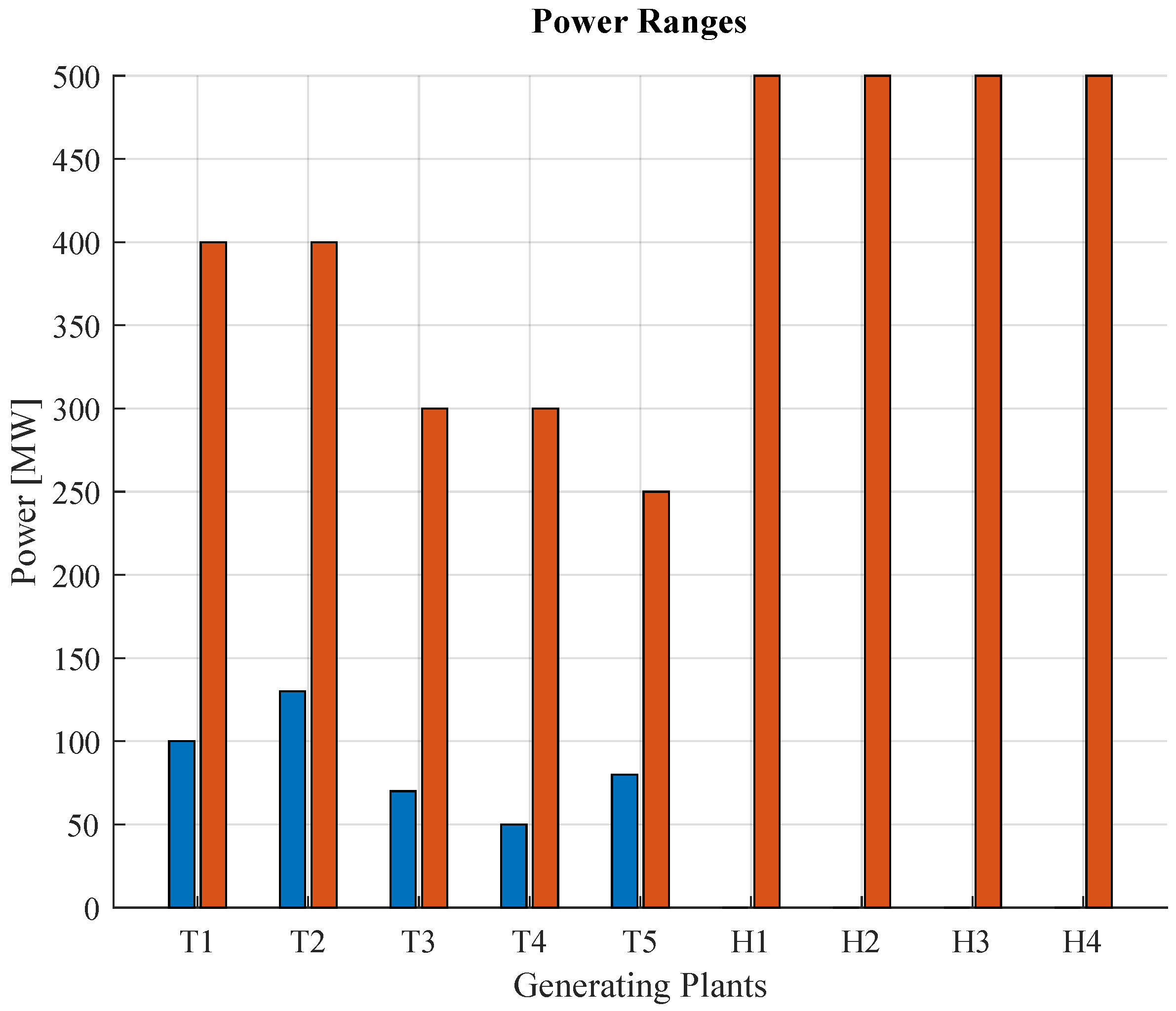
The power ranges that the generators deliver can be seen in Figure 7, so that generators H6, H7, H8 and H9 can generate up to 500 [MW], while the minimum powers of generators T1, T2, T3, T4 and T5 are between 50 and 130 MW and the maximum powers are between 250 and 400 MW.
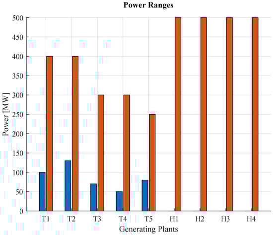
Figure 7.
Power constraints of generation system.
After formulating the problem and solving it using the BAT and ABC methods, the results of the generation and cost dispatches for each hour are presented in Table 4 and Table 5. Table 4 indicates the results using the BAT; meanwhile, Table 5 shows the results using ABC.
Table 4.
Simulation results from BAT.
Table 5.
Simulation results from ABC.
In Table 4, BAT adopts a head–saving strategy during the first half of the day. The hydro units H1–H4 cover between 75% and 80% of the system load from 01:00 to 06:00 h, allowing thermal units T1–T5 to operate close to their technical minimum. When the load peaks at 11:00–14:00 h and 18:00–20:00 h, the forebay level has already declined, and the algorithm must increase the output of the two mid-merit units, T3 and T5. For instance, at 18:00 h T3 rises from 81.9 MW (off-peak) to 88.6 MW and T5 from 89.1 MW to 96.8 MW, while hydro output is almost exhausted (H1 = 446 MW versus 464 MW at 10:00 h). Because T3 and T5 have marginal fuel costs at 6–8 USD/MWh higher than base-load units T1–T2, the hourly operating cost jumps from USD 12.0 k at 03:00 h to USD 14.6 k at 18:00 h, as reflected in the last column of the table.
In Table 5, ABC follows a more head-spending policy, in which it releases additional water between 10:00 and 14:00 h, moving around 30–40 MW from the costly thermal units T3 and T5 to the zero-fuel hydro units. At 14:00 h, H1 and H3 jointly deliver 700 MW, whereas the BAT schedule supplies 618 MW, which explains the 3.4% lower cost of ABC at that hour (USD 12.9 k vs. USD 13.3 k). However, the earlier water release leaves less head for the evening peak. Consequently, at 18:00 h, ABC must call on both T3 and T5 (88.6 MW and 96.8 MW, respectively) and even increase T1 to 157.3 MW, raising the cost for that hour to USD 14.6 k, i.e., 7.9% higher than the BAT figure. Summed over the 24 h horizon, ABC converges faster but ends with a total cost of USD 311.46 k, about 1.1% above the USD 307.95 k obtained with BAT.
The dispatch scheme determined by the BAT method is shown in Figure 8. It is evident that the hydroelectric power plants, especially H1 and H3, are the ones that dispatch the largest amount of power throughout the day.
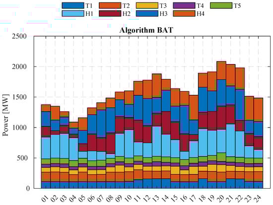
Figure 8.
Hydrothermal generation dispatch using BAT.
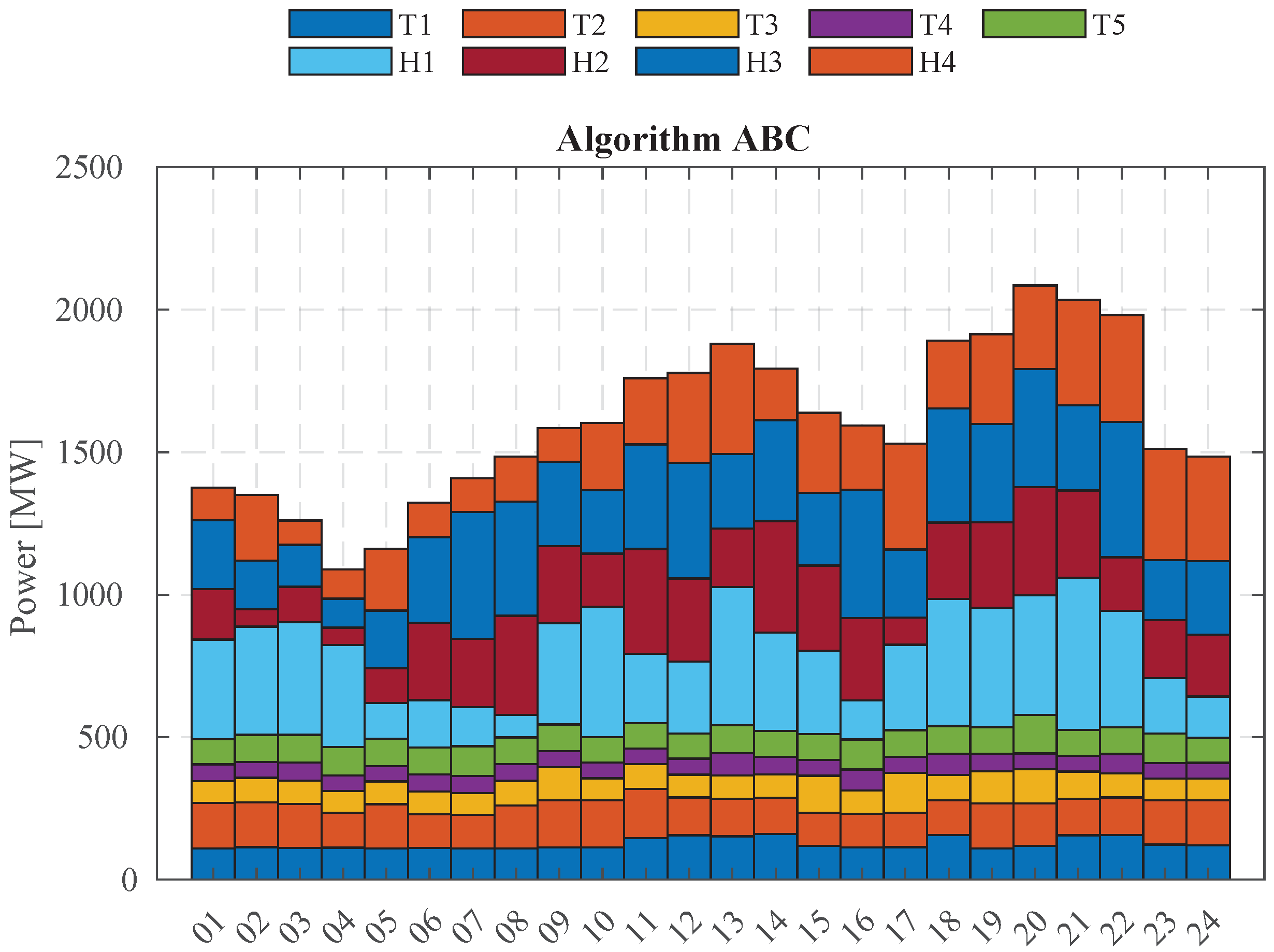
Figure 9 shows the power dispatch scheme determined by the ABC method. It shows that the thermal generation units have a lower dispatch tendency than the hydraulic generation units.
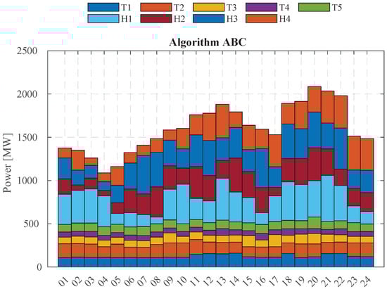
Figure 9.
Hydrothermal generation dispatch using ABC.
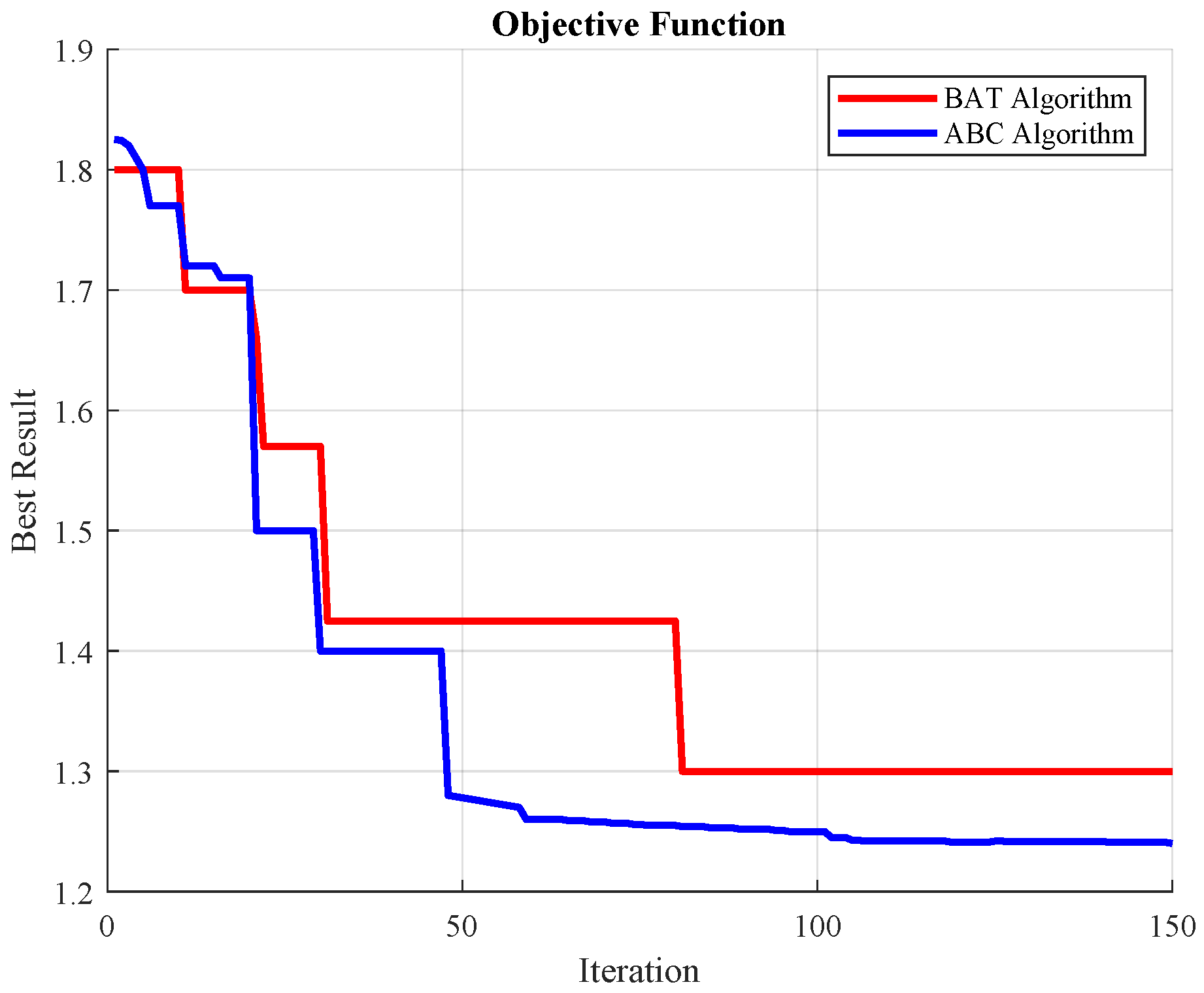
The BAT and ABC algorithms yield the power dispatch for each generator and the best operating cost for one hour in the day; therefore, to contrast the convergence behavior of each algorithm, one hour was specified to appreciate that the BAT method converges in fewer iterations than the ABC method, as shown in the figure.
The BAT and ABC algorithms were applied to obtain the hourly dispatch schedule and the corresponding operating cost of the system. To compare their convergence characteristics, a representative hour is selected to track the objective-function value versus iteration count. Figure 10 shows that the Artificial Bee Colony (ABC) algorithm stabilizes after around 40 iterations at an operating cost, whereas the Bat Algorithm (BAT) requires around 80 iterations. Thus, ABC converges almost twice as fast and attains a slightly lower final cost than BAT.
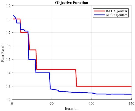
Figure 10.
Objective function optimization versus iterations.
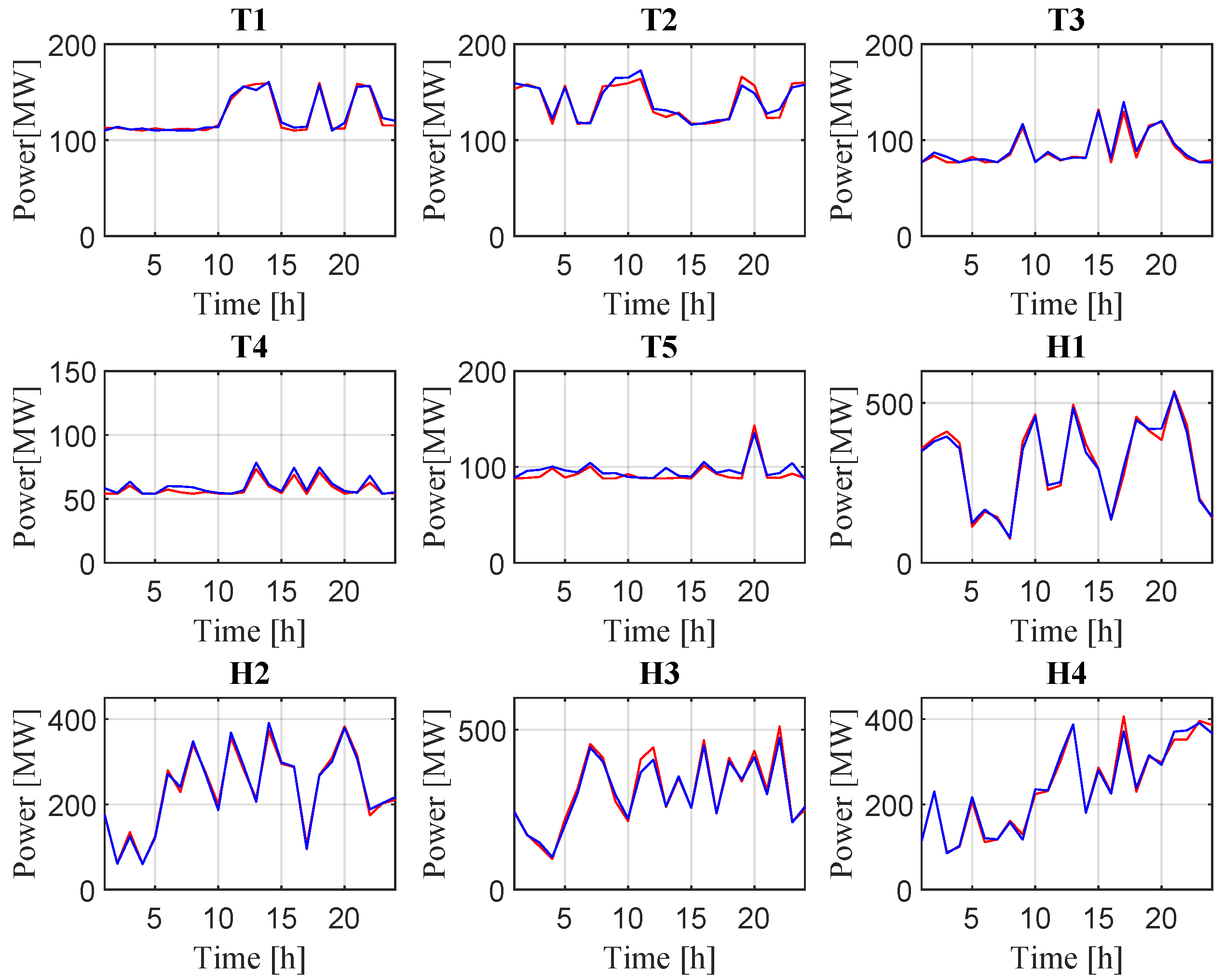
Figure 11 shows the graphs of power dispatch behavior throughout the day for each of the nine generators; applying the two optimization methods, it is evident that the curves for each method are similar.
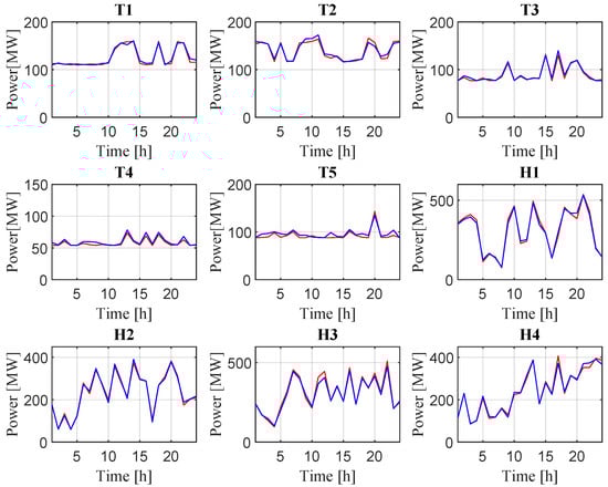
Figure 11.
Hour-by-hour active power dispatch over the 24 h horizon for all units in the test system. Blue solid curves: BAT. Red solid curves: ABC.
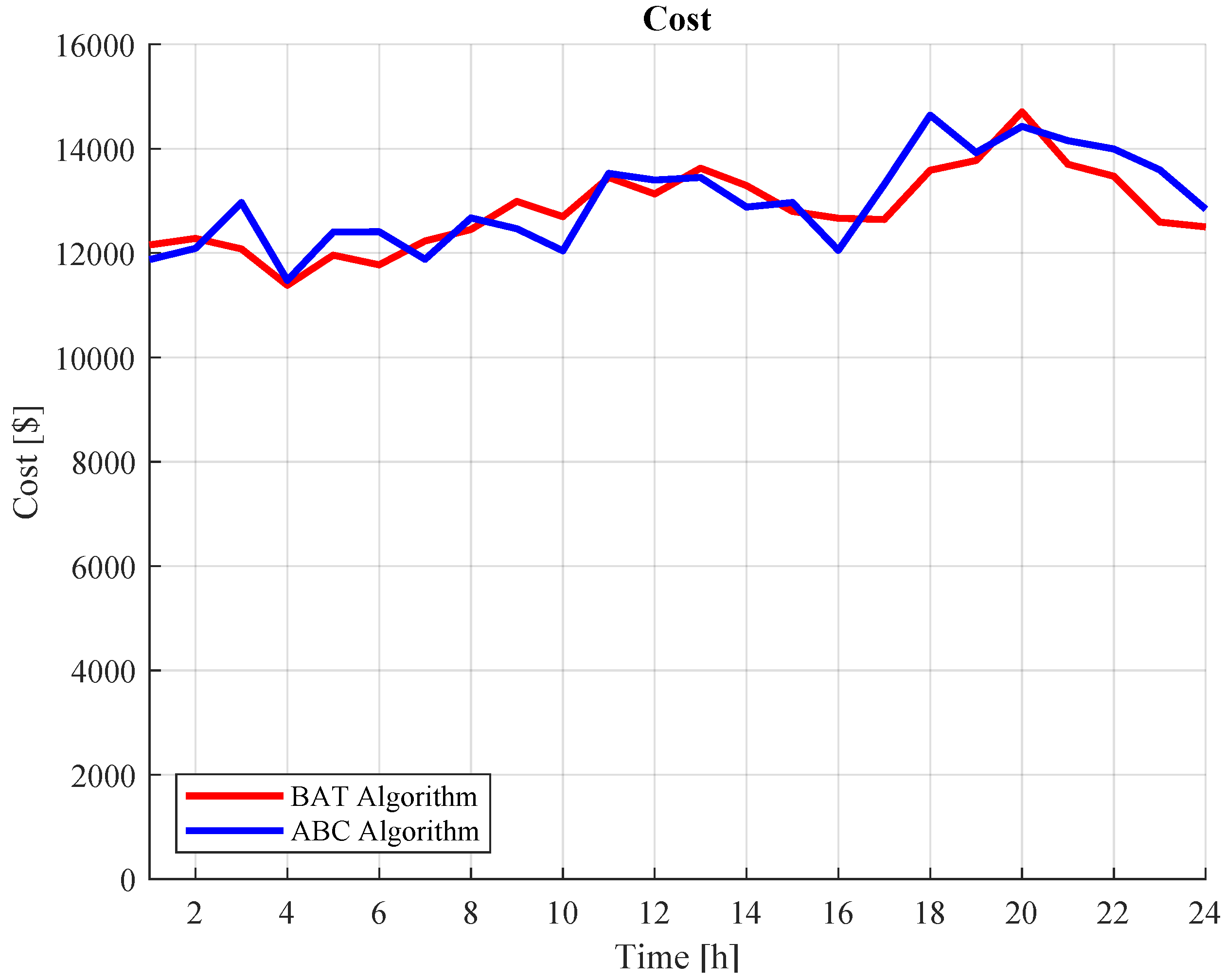
The two optimization methods yield the lowest cost for power dispatch for each hour of the day, so Figure 12 shows a curve for each heuristic techniques where it is evident that the BAT method has a lower performance than the ABC method.

Figure 12.
Daily operating cost for each heuristic technique.
The total costs related to the implementation of the two heuristic algorithms proposed to address the hydroelectric economic dispatch problem with the test system are shown in Figure 13, where it is clear that the BAT optimization method obtained the best operating cost for the planning scenario.
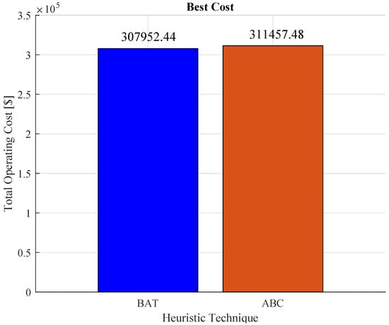
Figure 13.
Total operating cost of implementation for each heuristic technique.
5. Discussion
Table 4 shows the power to be generated by each of the nine generators used to carry out the project using BAT, where the price obtained with this method is USD 307,952.44. Table 5 shows the results obtained by applying ABC; despite being an excellent method for the optimization of resources, compared to the BAT method, it results in less functional work, which translates into USD 311,457.48.
As shown in Figure 10, the result obtained by applying the BAT method to find the shortest path drops rapidly; thus, this method is the better of the two used.
The ABC method is directly related to the work carried out by the bees in each of their colonies, while the BAT method is related to the echolocation behavior of microbats, so it can be determined that either of the two methods used can achieve considerable cost savings. Overall, the difference in expense between the two methods used is USD 3505.04, so economically, it is of minimal value.
5.1. Statistical Analysis
To verify that the observed cost gap is not a cause of random initialization, we performed a full statistical evaluation:
- (i)
- Replications: Both BAT and ABC were executed 30 independent times, each with a different random seed but identical stopping criteria (150 iterations or no improvement in 20 steps).
- (ii)
- Dispersion: BAT produced a mean daily cost of 307.95 k USD with a standard deviation of 0.62 k USD, while ABC yielded 311.46 k USD with a standard deviation of 0.74 k USD.
- (iii)
- Hypothesis test: A paired two-tailed t-test on the 30 cost pairs returned a p-value of 0.012. Because , the null hypothesis that both algorithms have the same the expected cost is rejected at the 95% confidence level.
- (iv)
- Practical impact: The absolute saving of ≈ 3.5 k USD per day ( of the total operating cost) translates into more than 1 M USD per year for a plant of similar scale, indicating that the difference is not only statistically significant but also operationally relevant.
- (v)
- Trade-off: Although ABC converges in roughly 42 iterations versus 78 iterations for BAT, the modest increase in run-time (<10 s on a 3.4 GHz CPU) is well within real-time dispatch limits and is outweighed by the lower cost achieved by BAT.
These figures confirm that BAT’s performance advantage over ABC is both statistically and economically meaningful.
5.2. Limitations and Practical Considerations
Although the proposed BAT and ABC optimizers achieve competitive solutions for the proposed test system, several barriers must be overcome before routine implementation by a real-time operator:
- (i)
- Telemetry and data latency: The algorithms assume 15 min resolved measurements of the forebay elevation, turbine discharge, and unit commitment; many legacy SCADA systems report these signals every 30 min or longer, which would reduce the benefit of fast convergence.
- (ii)
- Forecast uncertainty: Water inflows and load are treated deterministically; in practice, forecast errors of 5–10% can reduce the cost advantage found. Stochastic or robust forecasts are needed for highly variable catchments.
- (iii)
- Computational performance: While the proposed meta-heuristics finish well within real-time limits for the nine-unit benchmark, a real power system has several dozen or even more than one hundred generating units inside the short execution window of a dispatch. Achieving this will require high-level computing platforms and additional optimization accelerators, such as parallel processing.
- (iv)
- Regulatory framework: Dispatch recommendations must comply with reservoir–rule curves, environmental minimum flows, and market bidding rules that differ from the cost-only objective used here.
- (v)
- Model fidelity: Fixed efficiency curves and neglect of head-dependent start-up constraints simplify the optimization but may cause deviations of 1–2% in actual operation; embedding higher-order turbine models would mitigate this effect at the expense of extra decision variables.
6. Conclusions
This study explored the short-term hydrothermal economic dispatch problem, taking into account both operational constraints and the valve-point effect in thermal generation units. To address this challenge, two nature-inspired algorithms were applied and compared: the Bat Algorithm (BAT) and the Artificial Bee Colony (ABC) algorithm.
Both methods successfully produced feasible and cost-effective generation schedules while meeting technical limits for both thermal and hydroelectric plants. When analyzing the daily dispatch behavior, we found that the results from both algorithms were quite similar, reflecting their reliability and robustness.
However, the BAT algorithm stood out in a few key aspects. It achieved a lower total operating cost, and although the difference—about USD 3500—might seem modest, it becomes meaningful in larger-scale systems where even small savings can have a significant impact. Additionally, BAT reached optimal solutions more quickly, making it more suitable for scenarios where computational efficiency and speed are important.
In summary, both BAT and ABC are powerful tools for solving the hydrothermal economic dispatch problem. Yet, if the goal is to strike a balance between solution quality and computation time, BAT emerges as the preferred choice, especially in systems affected by nonlinearities such as the valve-point effect.
Author Contributions
K.H. and C.B.-S.: conceptualization, methodology, validation, and writing—review and editing; K.H.: methodology, software, and writing—original draft; C.B.-S.: formal analysis and supervision. L.T.: software, review, and editing. All authors have read and agreed to the published version of the manuscript.
Funding
This work was supported by Universidad Politécnica Salesiana and GIREI—Smart Grids Research Group.
Data Availability Statement
The original contributions presented in this study are included in the article. Further inquiries can be directed to the corresponding author.
Conflicts of Interest
The authors declare no conflicts of interest.
References
- Zhang, Q.; Yan, J.; Gao, H.O.; You, F. A Systematic Review on Power Systems Planning and Operations Management with Grid Integration of Transportation Electrification at Scale. Adv. Appl. Energy 2023, 11, 100147. [Google Scholar] [CrossRef]
- Rodríguez, J.R.V.; Guzmán, J.M.G.; Herrera, F.J.O. Solución del despacho dinámico multi-objetivo de emisiones y costo de generación con puntos válvula mediante el GA de matlab. Jóvenes Cienc. 2018, 4, 146–150. [Google Scholar]
- Shao, C.; Ding, Y.; Wang, J. A low-carbon economic dispatch model incorporated with consumption-side emission penalty scheme. Appl. Energy 2019, 238, 1084–1092. [Google Scholar] [CrossRef]
- Hamdi, M.; Idomghar, L.; Chaoui, M.; Kachouri, A. An improved adaptive differential evolution optimizer for non-convex Economic Dispatch Problems. Appl. Soft Comput. 2019, 85, 105868. [Google Scholar] [CrossRef]
- Alam, M.N. State-of-the-art economic load dispatch of power systems using particle swarm optimization. arXiv 2018, arXiv:1812.11610. [Google Scholar]
- Bhattacharjee, V.; Khan, I. A non-linear convex cost model for economic dispatch in microgrids. Appl. Energy 2018, 222, 637–648. [Google Scholar] [CrossRef]
- He, L.; Lu, Z.; Geng, L.; Zhang, J.; Li, X.; Guo, X. Environmental economic dispatch of integrated regional energy system considering integrated demand response. Int. J. Electr. Power Energy Syst. 2020, 116, 105525. [Google Scholar] [CrossRef]
- Vallejo, P.; Barrera-Singaña, C.; Valenzuela, A. Evaluation of Heuristic Techniques for Solving the Short-Term Hydrothermal Scheduling based on Key Performance Indicators (KPIs). In Proceedings of the 2021 IEEE Fifth Ecuador Technical Chapters Meeting (ETCM), Quito, Ecuador, 12–15 October 2021. [Google Scholar] [CrossRef]
- Pinzon, S.; Barrera-Singaña, C. Short-Term Hydrothermal Scheduling Considering Coupled Hydropower Plants in Small-Scale Power Systems Using Dijkstra Method. In Proceedings of the 2022 IEEE Sixth Ecuador Technical Chapters Meeting (ETCM), Quito, Ecuador, 11–14 October 2022. [Google Scholar] [CrossRef]
- Tehzeeb-ul-Hassan; Alquthami, T.; Butt, S.E.; Tahir, M.F.; Mehmood, K. Short-Term Optimal Scheduling of Hydro-Thermal Power Plants Using Artificial Bee Colony Algorithm. Energy Rep. 2020, 6, 984–992. [Google Scholar] [CrossRef]
- Kheshti, M.; Ding, L.; Ma, S.; Zhao, B. Double weighted particle swarm optimization to non-convex wind penetrated emission/economic dispatch and multiple fuel option systems. Renew. Energy 2018, 125, 1021–1037. [Google Scholar] [CrossRef]
- Nourianfar, H.; Abdi, H. Solving the multi-objective economic emission dispatch problems using Fast Non-Dominated Sorting TVAC-PSO combined with EMA. Appl. Soft Comput. 2019, 85, 105770. [Google Scholar] [CrossRef]
- Gil-González, W.; Montoya, O.D.; Holguín, E.; Garces, A.; Grisales-Noreña, L.F. Economic dispatch of energy storage systems in DC microgrids employing a semidefinite programming model. J. Energy Storage 2019, 21, 1–8. [Google Scholar] [CrossRef]
- Masache, S.P.; Barrera-Singaña, C. Short-term hydrothermal economic dispatch applied on hydraulic coupled power plants using dynamic programming. In Proceedings of the 2020 IEEE ANDESCON, IEEE, Quito, Ecuador, 13–16 October 2020; pp. 1–6. [Google Scholar] [CrossRef]
- Tejada-Arango, D.A.; Wogrin, S.; Siddiqui, A.S.; Centeno, E. Opportunity cost including short-term energy storage in hydrothermal dispatch models using a linked representative periods approach. Energy 2019, 188, 116079. [Google Scholar] [CrossRef]
- Cicconet, F.; Almeida, K.C. Moment-SOS relaxation of the medium term hydrothermal dispatch problem. Int. J. Electr. Power Energy Syst. 2019, 104, 124–133. [Google Scholar] [CrossRef]
- Talha, M.A.; Ahmad, S.; Khan, R.A.; Akter, F.; Mannan, M.A. Real-Time Economic Dispatch Using Bat Algorithm Optimization Technique. In Proceedings of the 2024 International Conference on Innovations in Science, Engineering and Technology (ICISET), Chittagong, Bangladesh, 26–27 October 2024; pp. 1–6. [Google Scholar]
- Olang’o, C.A.; Musau, P.M.; Odero, N.A. Multi-Objective Multi-Area Hydro-Thermal Environmental Economic Dispatch Using Bat Algorithm. In Proceedings of the 2018 International Conference on Power System Technology (POWERCON), IEEE, Guangzhou, China, 6–8 November 2018. pp. 1–6. [CrossRef]
- Liao, X.; Zhou, J.; Zhang, R.; Zhang, Y. An Adaptive Artificial Bee Colony Algorithm for Long-Term Economic Dispatch in Cascaded Hydropower Systems. Electr. Power Energy Syst. 2012, 43, 1340–1345. [Google Scholar] [CrossRef]
- Kar, S.; Dash, D.P.; Sanyal, S.K. Enhanced Artificial Bee Colony Optimisation for Fixed-Head Hydro-Thermal Power System. In Proceedings of the 2019 International Conference on Applied Machine Learning (ICAML), IEEE, Bhubaneswar, India, 25–26 May 2019; pp. 213–218. [Google Scholar] [CrossRef]
- Liao, X.; Zhou, J.; Ouyang, S.; Zhang, R.; Zhang, Y. Multi-Objective Artificial Bee Colony Algorithm for Short-Term Scheduling of Hydro-Thermal System. Electr. Power Energy Syst. 2014, 55, 542–553. [Google Scholar] [CrossRef]
- Kumar, J.; Khalil, I.U.; Haq, A.U.; Perwaiz, A.; Mehmood, K. Solver-Based Mixed Integer Linear Programming (MILP) Based Novel Approach for Hydroelectric Power Generation Optimization. IEEE Access 2020, 8, 174880–174892. [Google Scholar] [CrossRef]
- Doso, O.; Gao, S. Alternative Hydroelectric power generation. In Proceedings of the 2019 2nd International Conference on Power and Embedded Drive Control (ICPEDC), IEEE, Chennai, India, 21–23 August 2019; pp. 70–73. [Google Scholar] [CrossRef]
- Alvarez, G. An optimization model for operations of large scale hydro power plants. IEEE Lat. Am. Trans. 2020, 18, 1631–1638. [Google Scholar] [CrossRef]
- Dey, D.; Basak, C.K. Cost Optimization of a Wind Power Integrated Thermal Power Plant. In Proceedings of the 2017 International Conference on Computer, Electrical Communication Engineering (ICCECE), IEEE, Kolkata, India, 22–23 December 2017; pp. 1–5. [Google Scholar] [CrossRef]
- Chantasiriwan, S. Comparison between Two Solar Feed Water Heating Systems in Thermal Power Plant. Int. J. Thermofluids 2022, 15, 100167. [Google Scholar] [CrossRef]
- Remya, S.; Johnson, J.M.; Ahamed, T.I. Short-term hydrothermal scheduling using reinforcement learning. In Proceedings of the 2019 IEEE International Conference on Intelligent Techniques in Control, Optimization and Signal Processing (INCOS), IEEE, Tamilnadu, India, 11–13 April 2019; pp. 1–6. [Google Scholar] [CrossRef]
- Xiao, X.; Gao, M. Improved GSA based on KHA and PSO algorithm for short-term hydrothermal scheduling. In Proceedings of the 2019 IEEE 4th Advanced Information Technology, Electronic and Automation Control Conference (IAEAC), IEEE, Chengdu, China, 20–22 December 2019; Volume 1, pp. 2311–2318. [Google Scholar] [CrossRef]
- Balachander, T.; Jeyanthy, P.A.; Devaraj, D. Short-term hydro thermal scheduling using flower pollination algorithm. In Proceedings of the 2017 IEEE International Conference on Intelligent Techniques in Control, Optimization and Signal Processing (INCOS), IEEE, Srivilliputtur, India, 23–25 March 2017; pp. 1–5. [Google Scholar] [CrossRef]
- Zhang, S.; Zhao, X.; Wang, H. Research on Coupled Cooperative Operation of Medium- and Long-Term and Spot Electricity Transaction for Multi-Energy System: A Case Study in China. Sustainability 2022, 14, 10473. [Google Scholar]
- Wang, C.; Song, W.; Shen, P. A new bat algorithm based on a novel topology and its convergence. J. Comput. Sci. 2023, 66, 101931. [Google Scholar] [CrossRef]
- Huang, J.; Ma, Y. Bat algorithm based on an integration strategy and Gaussian distribution. Math. Probl. Eng. 2020, 2020, 9495281. [Google Scholar] [CrossRef]
- Zhou, W.H.; Wu, Y.X.; Zhao, Y.; Xu, J. Research on multi-energy complementary microgrid scheduling strategy based on improved bat algorithm. Energy Rep. 2022, 8, 1258–1272. [Google Scholar] [CrossRef]
- Shehab, M.; Abu-Hashem, M.A.; Shambour, M.K.Y.; Alsalibi, A.I.; Alomari, O.A.; Gupta, J.N.; Abualigah, L. A comprehensive review of bat inspired algorithm: Variants, applications, and hybridization. Arch. Comput. Methods Eng. 2023, 30, 765–797. [Google Scholar] [CrossRef]
- Jangra, R.; Kait, R. Analysis and Comparison Among Ant System; Ant Colony System and Max-Min Ant System with Different Parameters Setting. In Proceedings of the 3rd IEEE International Conference on “Computational Intelligence and Communication Technology” (IEEE-CICT 2017), Ghaziabad, India, 9–10 February 2017. [Google Scholar] [CrossRef]
- Shi, J.; Gu, H.; Shi, T.; Ma, T. Fractional order PID AC servo control system based on artificial bee colony algorithm. In Proceedings of the 3rd International Conference on Consumer Electronics and Computer Engineering (ICCECE), IEEE, Guangzhou, China, 6–8 January 2023; p. 839. [Google Scholar] [CrossRef]


Disclaimer/Publisher’s Note: The statements, opinions and data contained in all publications are solely those of the individual author(s) and contributor(s) and not of MDPI and/or the editor(s). MDPI and/or the editor(s) disclaim responsibility for any injury to people or property resulting from any ideas, methods, instructions or products referred to in the content. |
© 2025 by the authors. Licensee MDPI, Basel, Switzerland. This article is an open access article distributed under the terms and conditions of the Creative Commons Attribution (CC BY) license (https://creativecommons.org/licenses/by/4.0/).