Impact of Passive Modifications on the Efficiency of Darrieus Vertical Axis Wind Turbines Utilizing the Kline-Fogleman Blade Design at the Trailing Edge

Abstract

As the utilization of wind energy continues to expand as a prominent renewable energy source, the application of Darrieus Vertical Axis Wind Turbine (VAWT) technology has expanded significantly. Various passive modification methods have been developed to enhance efficiency and optimize the aerodynamic performance of the rotor through blade modifications. This study presents passive modification method utilizing Kline–Fogleman (KF) blades which incorporate step-like horizontal slats along the trailing edge. Through Computational Fluid Dynamics (CFD) simulations, this study evaluates ten distinct KF blade configurations, varying in step length and depth, with steps positioned on the inner side, outer side, and both sides of the airfoil. The results indicate that the KF blade with a shorter step on inner side, 20%$c$ in length and 2%$c$ in depth, enhances the average power coefficient ($C_p$) by 19% compared to the rotor with a clean blade. However, when horizontal slats are incorporated on both sides of the blade, with dimensions of 50%$c$ in length and 5%$c$ in depth, $C_p$ decreases by 33% compared to the clean blade. This reduction occurs across both low and high tip speed ratio (TSR) ranges. It has been observed that the presence of a high-pressure zone of 200 Pa at the trailing edge disrupts the aerodynamic performance when the KF blade is in the upwind region between the azimuth angles of 45° and 135°.

1. Introduction

The recent alarming rise in air pollution and carbon emissions from fossil fuel consumption has significantly accelerated the development of renewable energy sources such as solar, wind, and biomass. Among these, wind energy stands out as a reliable, widely accessible, and cost-effective alternative for clean power generation [1]. Advances in wind energy technology have led to the evolution of wind turbines. Based on their axis of rotation, wind turbines can be categorized into two primary groups: Horizontal Axis Wind Turbines (HAWTs) and Vertical Axis Wind Turbines (VAWTs). VAWTs, which exhibit independence from wind direction and require relatively low maintenance, have recently become a reliable option for urban wind power systems [2].

VAWTs are classified based on the predominant aerodynamic force driving their rotation. These include lift-based rotors, such as H-type Darrieus VAWTs and helical Gorlov VAWTs, and drag-based rotors, commonly known as impulse rotors, such as Savonius type [3]. Lift-based rotors are known for their capacity to deliver higher output power and operate effectively at high tip speed ratios (TSRs). However, they suffer from low torque at low TSRs, making self-starting difficult [4]. In contrast, drag-based rotors function primarily in the low-TSR range and are self-starting. Nevertheless, their power coefficient ($C_p$) declines significantly at higher ranges, limiting their suitability for urban installations [5]. Although lift-based rotors, particularly H-type Darrieus VAWTs, demonstrate an acceptable $C_p$ in the high-TSR range, there is growing interest in enhancing their efficiency through improvements in aerodynamic performance achieved via blade modifications, which are categorized as passive techniques. The primary goal of these blade modifications is to improve both torque and lift across different blade positions throughout the rotor’s rotation [6].

A notable blade modification technique involves the implementation of slotted blades, which make a significant advancement among passive methodologies. This approach effectively improves airflow dynamics by drawing air from the leading edge and pressure side, while concurrently discharging airflow from the suction side and trailing edge [7]. This modification can improve $C_p$ by as much as 10% in the high-TSR range. However, it is important to note that $C_p$ may decrease by up to 18.5% in the low-TSR range, primarily due to flow separation on the blade surfaces [8]. Implementing vortex cavity layers on both the outer and inner sides of blades may represent another viable blade modification technique. These layers’ strategic positioning and spacing are critical, as they can significantly influence flow attachment and separation on the blade’s suction side, particularly near the trailing edge [9]. Placing a vortex cavity in the middle of the suction side can delay dynamic stall by generating swirling flow at high angles of attack (AoA), potentially enhancing $C_p$ by 64% in the low-TSR range and by 3% in high-TSR range [10].

A significant body of research examines passive modifications to the blade near the trailing edge to improve lift force at high AoA. These enhancements are primarily achieved through the integration of either movable or stationary flaps situated on the pressure and suction sides adjacent to the trailing edge, as well as through the use of J-shaped blades featuring openings from the trailing edge and vertical or horizontal slots positioned near the trailing edge [11]. Implementing a J-shaped blade airfoil profile, instead of the clean airfoil profile, has significantly enhanced blade torque, achieving an increase of 49.5% within the low-TSR range. This modification highlights the advantages of innovative design in optimizing performance metrics [12]. Also, compared to a rotor with a clean blade design, J-shaped blade airfoil profiles have improved the $C_p$ by up to 25% when the spanwise opening from the trailing edge is adjusted to 70% of the chord [13]. The gurney flap (GF), implemented as a vertical plane at the trailing edge tip, can generate vortices and enhance the rotor’s aerodynamic efficiency. This innovation can result in a 19% increase in blade torque [14]. Also, Zhu et al. [15] demonstrated that shorter GFs yield superior performance to their longer counterparts, as they can enhance $C_p$ by 21% in the high-TSR range. In a comparison of GF with a length ranging from 15% to 25% of the chord length and deflection angles of 90° to 120°, GF with a 15% chord length and a deflection angle of 120° demonstrated superior $C_p$compared to the clean blade at TSR = 2.5 [16]. Chen et al. [17] showed that the serrated gurney flap enhanced the $C_p$ by 13.9% within a high-TSR range (TSR > 2.5) compared to the clean GF. This improvement is due to the increased annular velocity, which results in greater vortices that enhance lift forces. Conversely, the simple type exhibited superior performance within the low-TSR range. Syawitri et al. [18] demonstrated that the vertically slotted GF can enhance the $C_p$ by 1.5% in the low-TSR range and 11.3% in the high-TSR range compared to the clean GF. Han et al. [19] demonstrated the feasibility of a movable flap with pitch angle control. The results indicated that the optimal flap length is 95% of the chord, with a pitch angle ranging from 10 to 15, which is the most effective within a high-TSR range.

One passive flow control technique involves incorporating horizontal slats near the trailing edge on the outer or inner sides and implementing backward-facing step geometry on the airfoil surface. This design, commonly referred to as Kline–Fogleman (KF) airfoils, was developed by Richard Kline and Floyd Fogleman in the 1960s and has been primarily applied to aircraft wings [20]. KF airfoils, with single or multiple steps, can significantly enhance lift by approximately 20% to 30%, with particularly notable improvements in delaying stall, thereby boosting overall aerodynamic performance [21]. The depth, angle, and number of steps in blades are critical factors affecting KF airfoil aerodynamic performance, as they influence flow attachment and separation. These phenomena can be evaluated through flow visualization on the blade surface and by analyzing the width of the wake region downstream of the blade [22]. Iddou et al. [23] found that a KF airfoil with steps on both the outer and inner sides of NACA0015 can enhance $C_p$ compared to a Darrieus rotor equipped with a clean blade. However, the study’s scope was confined to the KF blade configuration, which employed a fixed-size horizontal slot. It did not explore the impact of varying horizontal slot sizes at the blade’s trailing edge, nor did it assess the effects of different dimensions in both depth and length on aerodynamic performance.

This research introduces an innovative passive aerodynamic modification strategy for Darrieus VAWTs through the application of KF airfoil, an approach that to the best of our knowledge, has not previously been widely explored in depth within the context of lift-based VAWTs. In contrast to traditional blade modification techniques that primarily concentrate on altering camber, implementing vortex generators, or applying surface roughness treatments, this study investigates the use of slotted trailing-edge configurations inspired by the KF airfoil concept to passively influence flow behavior. The originality of this work is underscored by its comprehensive parametric framework, which rigorously assesses the aerodynamic implications of step dimensions and placements on both the blade’s inner and outer sides. Moreover, adapting KF principles to the VAWTs introduces a novel passive aerodynamic control mechanism capable of enhancing performance without the complications associated with additional mechanical systems or active control mechanisms. This methodology presents a cost-effective, structurally simple alternative to traditional enhancement techniques, thereby offering new avenues for improving VAWT efficiency and expanding the applications of passive flow control in wind energy technologies. It is essential to highlight that prior research has predominantly concentrated on the application of the KF blade on airplane wings and the potential for dynamic stall. In contrast, there has been a paucity of studies addressing the Darrieus VAWTs. Consequently, the influence of the KF blade on the aerodynamic performance of Darrieus VAWTs represents a considerable research gap, particularly regarding the systematic investigation of various parameters related to horizontal slot geometries. In particular, the effects of different locations, lengths, and depths of horizontal slots, as well as variations in slot positioning across different sizes on both the inner and outer surfaces of the blade, remain insufficiently examined. This study aims to bridge these gaps by focusing on the impact of the KF blade on the efficiency and self-starting capabilities of VAWTs.

2. Case Study Description

In this simulation, a two-dimensional model of the Darrieus rotor, as developed by Castelli et al. [24], serves as the control case. The Kline–Fogleman (KF) blade airfoil profile, which incorporates a horizontal step slat, is examined to enhance aerodynamic performance. These modifications are applied to the blade trailing edge following three distinct strategies: on the outer, inner, and both sides. The depth ($d$) and length ($l$) of the steps from the trailing edge are determined based on the chord length. The rotor dimensions and various configurations of the KF blades are outlined in

Table 1. Darrieus rotor dimensions.

Quantity	Value
Blade airfoil profile	NACA0021
Blade chord length ($c$)	85.8 (mm)
Rotor diameter ($D$)	1030 (mm)
Rotor solidity	0.5
Number of blades	3

and

Table 2. KF blade airfoil configurations.

Case Number	Location	$\mathit{l}/\mathit{c}$	$\mathit{d}/\mathit{c}$
Case 1	Inner side	20%	5%
Case 2	Inner side	20%	2%
Case 3	Inner side	50%	10%
Case 4	Inner side	50%	5%
Case 5	Outer side	20%	5%
Case 6	Outer side	20%	2%
Case 7	Outer side	50%	10%
Case 8	Outer side	50%	5%
Case 9	Both sides	50%	5%
Case 10	Both sides	20%	2%

, respectively, while the rotor schematic is illustrated in Figure 1.

According to Table 2, this study aims to investigate the effect of both the depth and length of KF blade steps on the rotor performance. Specifically, a length of 20%$c$ and 50%$c$ is considered, corresponding to lengths of 17 mm and 42 mm, respectively, from the trailing edge. In the case of the 20%$c$, the depths of 5%$c$ and 2%$c$ correspond to 4 mm and 2 mm, while for the case of the 50%$c$, the depths of 10%$c$ and 5%$c$ correspond to 8.5 mm and 4 mm, respectively. The rationale behind selecting the specified values for the KF blade step depth at 20%$c$ and 50%$c$ is rooted in the consideration of the airfoil profile thickness, as documented in NACA0021. Utilizing higher values for the depth compromises the blade’s structural integrity, resulting in a thinner configuration that diminishes its effectiveness in practical applications. Furthermore, values below 20%$c$ for the KF blade yield negligible effects for the step length, while lengths exceeding 50%$c$ of the trailing edge adversely affect strength and increase the likelihood of flow separation.

3. Governing Equations and Numerical Setup

This section discusses the governing equations based on the current simulation and the numerical setups applied to the CFD solver.

3.1. Fluid Mechanics Equations

The Unsteady Reynolds-Averaged Navier–Stokes (URANS) equation is utilized to characterize fluid flow dynamics near blades, facilitating a comprehensive and precise analysis of unsteady, turbulent fluid flow behavior. The formulation of the URANS equations for Newtonian incompressible flow relies on the assumption of a constant density that does not fluctuate with pressure variations. This approach is applicable when the blade tip tangential velocity remains below a Mach number of 0.3. This reinforces the fundamental assumption of incompressibility within the flow analysis presented herein. The URANS equation for incompressible flow is as follows [25]:

$${\displaystyle \frac{\partial \overline{u_i}}{\partial x_i}}=0$$

(1)

$${\displaystyle \frac{\partial \overline{u_i}}{\partial t}}+{\displaystyle \frac{\partial }{\partial x_j}}\left(\overline{{u_{i}u}_j}\right)=-{\displaystyle \frac{1}{\rho }}{\displaystyle \frac{\partial \overline{p}}{\partial x_i}}+{\displaystyle \frac{\partial }{\partial x_j}}\left(\nu {\displaystyle \frac{\partial \overline{u_i}}{\partial x_j}}-\overline{u_i^{\prime }{u}_j^{\prime }}\right)$$

(2)

The terms $\overline{u_i }(m/s)$ and $\overline{u_j} (m/s)$ show the Cartesian system’s mean velocity components, introducing the flow physics principle. The fluctuating velocities ${u\prime }_i (m/s)$ and ${u\prime }_j (m/s)$ are related to the capturing of turbulence effects. Also$\overline{p }(N/m^2)$, $\rho (kg/m^3)$, and $\nu (m^2/s)$ show the fluid’s governing pressure, density, and kinematic viscosity, respectively. $\rho \overline{u_i^{\prime }{u}_j^{\prime }}$ is defined as the Reynolds stress, representing the correlation between fluctuating quantities in velocity components. This characteristic offers valuable insights into the fluid’s complex turbulence-induced momentum transformations.

3.2. Turbulence Modeling Equations

Reynolds stress describes the complex fluid dynamics around rotor blades, making the choice of a suitable turbulence model essential for accurate simulations. Commonly used models include k−ε and k−ω, which are considered two-equation models based on two transport equations. Properly solving these equations is crucial for effectively modeling turbulent flows around blades. The selection of an appropriate turbulence model is essential for accurately simulating fluid flow around rotor blades. This decision necessitates a thorough understanding of the strengths and limitations of each model, as well as an assessment of its compatibility with the specific application context. The $k-\epsilon$ turbulence model is widely utilized in CFD due to its robustness and simplicity. This model integrates empirical damping functions to address near-wall effects within the viscous sublayer. However, this methodology often results in diminished accuracy in areas with adverse pressure gradients, consequently limiting its reliability in turbomachinery applications [26]. In contrast, the $k-\omega$ model demonstrates superior performance in near-wall regions without necessitating additional damping terms, thereby facilitating enhanced resolution of boundary layer phenomena. Nevertheless, its sensitivity to freestream turbulence characteristics, including turbulence intensity, restricts its predictive capabilities. The shear stress transport (SST) $k-\omega$ model has been developed as a hybrid framework to mitigate these limitations. This model combines the $k-\omega$ formulation near solid boundaries with the $k-\epsilon$ approach within the freestream, thus improving predictive accuracy across a broader spectrum of flow regimes, including those typical of turbomachinery environments [26]. Previous studies on CFD modeling of VAWTs indicate that the SST $k-\omega$ turbulence model may be the most accurate model available among RANS-based models for turbulent flow simulation around VAWT blades. This model provides more precise results compared to the one-equation Spalart–Allmaras model, which is more accurate for low-Reynolds number conditions and the two-equation models, such as the standard $k-\epsilon$ and standard $k-\omega$ models, as it effectively captures velocity fluctuations near the blades and accurately models velocity development in far-field regions [27,28]. According to this evidence, we will use the SST $k-\omega$ model for this simulation. In this simulation, turbulent kinetic energy (k) represents the energy in turbulent eddies and vortices. At the same time, the specific dissipation rate (ω) quantifies the rate at which this energy dissipates due to viscosity. The equations for $k (m^2/s^2)$ and $\omega \left(s^{-1}\right)$ are shown below [29].

$$\rho {\displaystyle \frac{d}{dt}}\left(k\right)+\rho \nabla ·\left[k\left(\overrightarrow{u}-{\overrightarrow{u}}_g\right)\right]=\nabla ·\left[\left(\mu +{\displaystyle \frac{{\mu }_t}{{\sigma }_k}}\right)\nabla k\right]+G_k-Y_k$$

(3)

$$\rho {\displaystyle \frac{d}{dt}}\left(\omega \right)+\rho \nabla ·\left[\omega \left(\overrightarrow{u}-{\overrightarrow{u}}_g\right)\right]=\nabla ·\left[\left(\mu +{\displaystyle \frac{{\mu }_t}{{\sigma }_{\omega }}}\right)\nabla \omega \right]+G_{\omega }-Y_{\omega }$$

(4)

Here, $Y_k \left({\displaystyle \frac{kg}{ m^3· s^3}}\right)$ and $G_k \left({\displaystyle \frac{kg}{ m^3. s^3}}\right)$ denotes the dissipation and generation of turbulent kinetic energy, respectively. $G_{\omega } \left({\displaystyle \frac{kg}{m^3· s^2}}\right)$ and $Y_{\omega } \left({\displaystyle \frac{kg}{m^3. s^2}}\right)$ are $\omega$ generation and dissipation, respectively. The turbulent Prandtl numbers for $k$ and $\omega$ are denoted by ${\sigma }_k$ and ${\sigma }_{\omega }$, respectively. ${\mu }_t$ is turbulent viscosity, computed from $k$ and $\omega$.

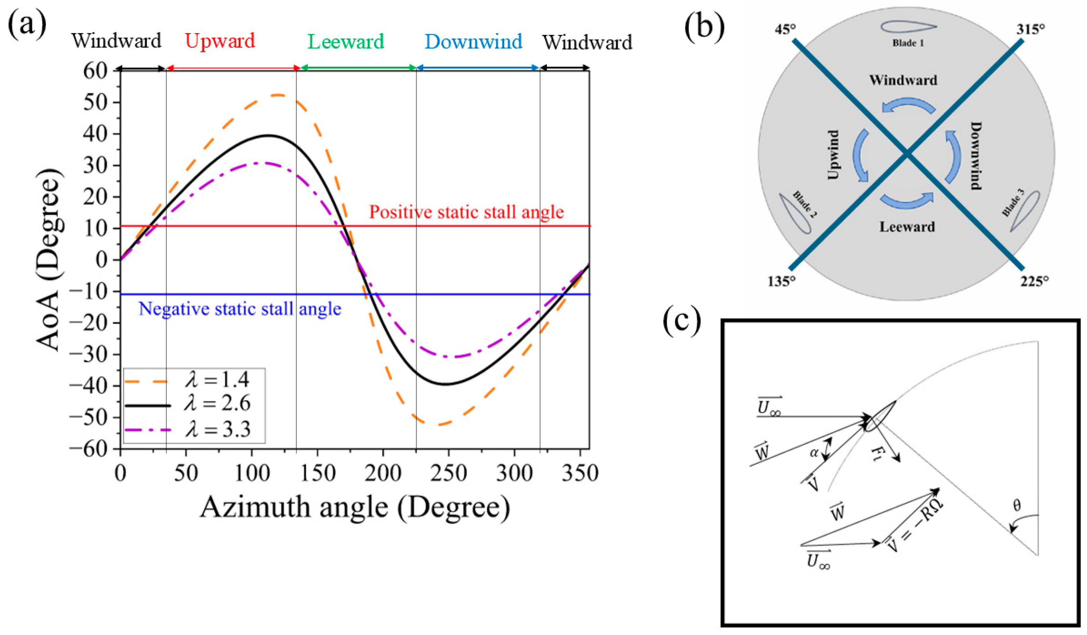
3.3. Turbine Mathematical Relations

The effectiveness of a rotor is determined by its power and torque, which are nondimensionalized as the torque coefficient ($C_m)$ and power coefficient $\left(C_p\right)$ as follows [30]:

$$C_p={\displaystyle \frac{P}{\frac{1}{2}\rho ·A·V_{\infty }^3}}$$

(5)

$$C_m={\displaystyle \frac{P}{\frac{1}{4}\rho ·D^2·H·V_{\infty }^2}}$$

(6)

where $P \left({\displaystyle \frac{N·m}{s}}\right)$ represents the rotor-generated power and is calculated by multiplying the turbine’s dynamic moment by its angular velocity $(\Omega \times M)$. $\rho \left({\displaystyle \frac{kg}{m^3}}\right)$ is air density, which is equal to 1.225 $\left({\displaystyle \frac{kg}{m^3}}\right)$, and $V_{\infty } \left({\displaystyle \frac{m}{s}}\right)$ is wind velocity towards the rotor. $A$ ($m^2$) is the swept area, which is achieved by multiplying the diameter ($D$) and height ($H)$. Considering the 2D approach, the turbine height is assumed equal to one.

An essential dimensionless parameter in the design process is the tip speed ratio (TSR), which represents the ratio of the tangential velocity of the blade tip to the incoming wind velocity. TSR is introduced as follows [30]:

$$\lambda ={\displaystyle \frac{R·\Omega }{V_{\infty }}}$$

(7)

where$\Omega \left({\displaystyle \frac{rad}{s}}\right)$ is the rotor angular velocity and $\mathrm{R}\left(\mathrm{m}\right)$ is the rotor radius.

Equation (8) establishes an analytical relationship between the azimuth angle and the angle of attack.

$$\alpha ={\tan }^{-1}\left({\displaystyle \frac{\sin \theta }{TSR+\cos \theta }}\right)$$

(8)

Here, $\theta$ is the azimuth angle, and $\alpha$ represents the angle of attack (AoA). In Figure 2, $\alpha$ is calculated as a function of the azimuth angle for three different TSRs.

According to Figure 2, which shows the variation of AoA over a turbine rotation, it is clear that the maximum and minimum AoA values demonstrate an inverse correlation with the TSR, a metric indicative of angular velocity. As TSR decreases, the operational range of AoA widens. The maximum and minimum AoA values are attained when the rotor is positioned in the upwind and downwind sections, respectively. Furthermore, as the blade approaches an AoA of 11°, which is close to the static stall angle, it indicates that the rotor undergoes a significant transition from the downwind to the windward area, particularly when the azimuth angle falls within the range of 300° to 360°. Under these circumstances, the rotor experiences an onset of the negative static stall angle. This phenomenon similarly occurs during the transition of the blade from the upwind to the leeward positions, with the azimuth angle ranging from 140° to 200°.

The $C_l$ values are determined using specific equations that assess the lift force resulting from variations in rotor rotation and changes in blade positioning, as illustrated by the velocity triangle in Figure 2c.

$$C_l={\displaystyle \frac{F_x\sin \left(\theta -\alpha \right)-F_y\cos \left(\theta -\alpha \right)}{\frac{1}{2}\rho ·A·V_{\infty }^2}}$$

(9)

The equation presented pertains to the normal force $F_y$and the tangential force $F_x$ acting upon the turbine blade. These forces have been calculated to ascertain the lift force, considering both the angles of attack and the azimuth angle.

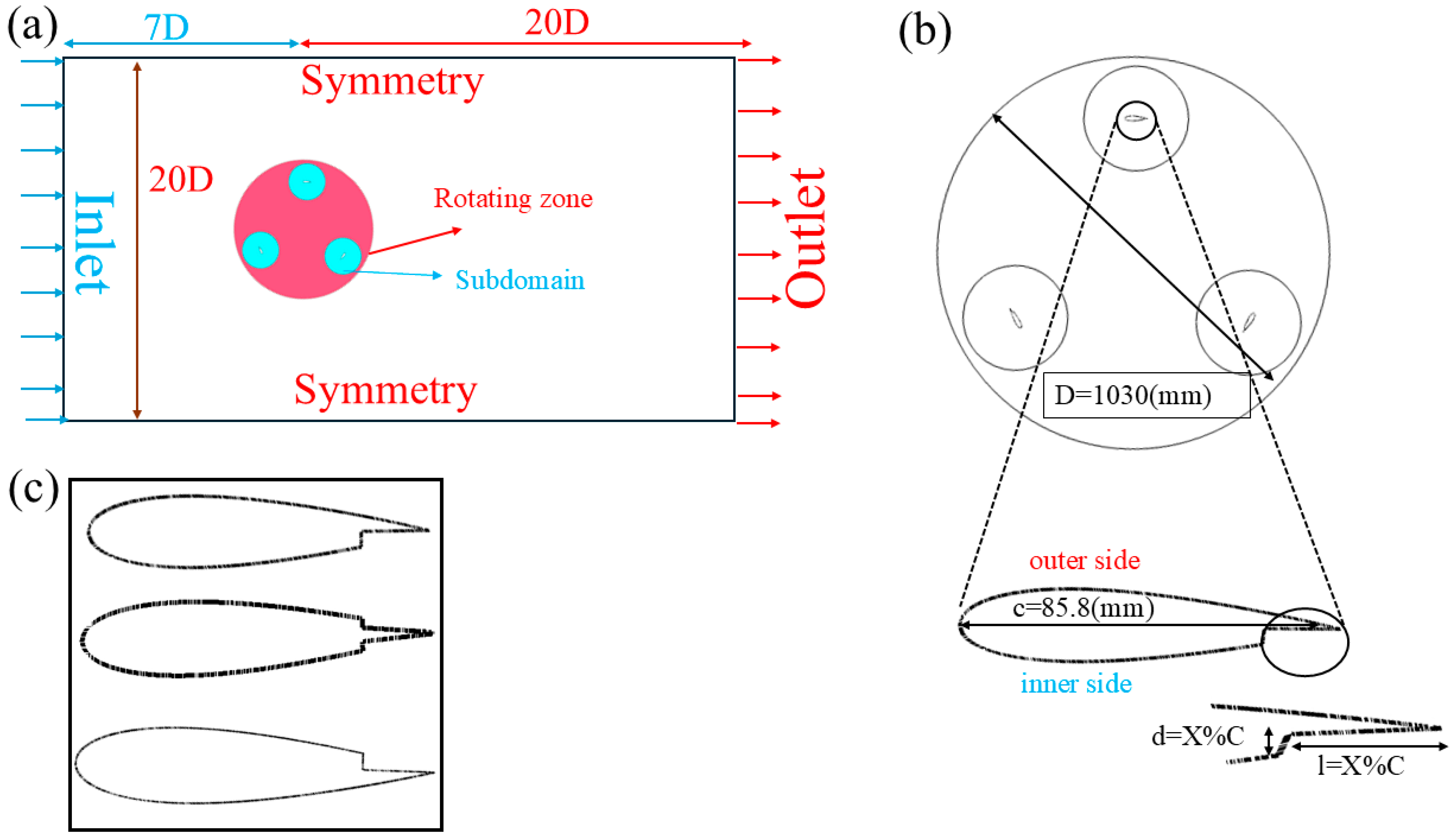
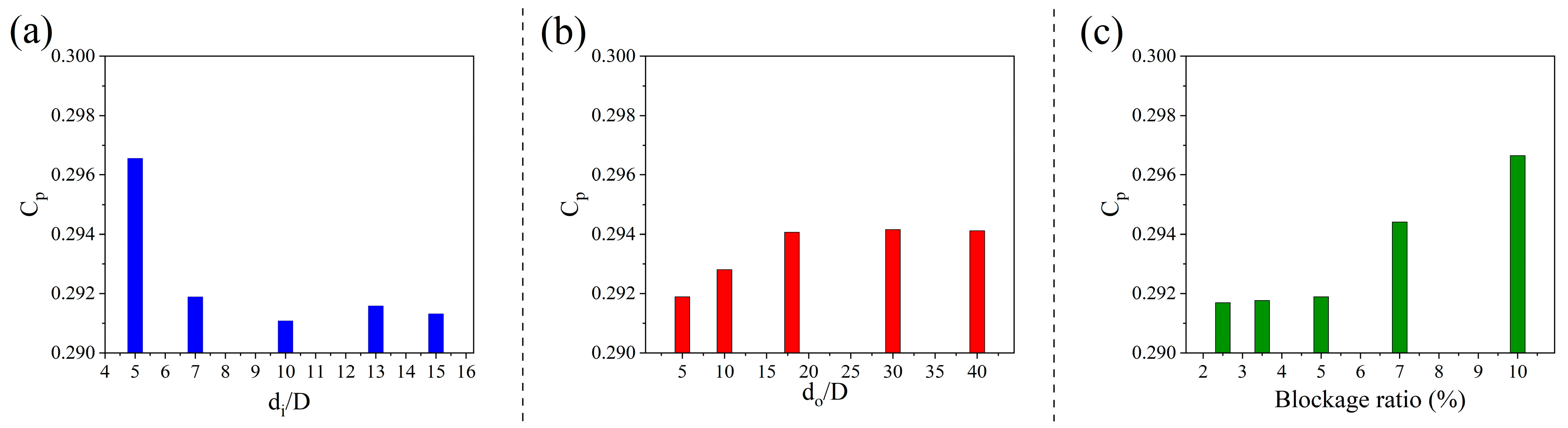
3.4. Computational Domain

In the present simulation, 2D CFD simulations were employed to investigate the flow dynamics surrounding the Darrieus rotor blades and the subsequent flow development in the rotor downstream area. The utilization of a 2D CFD model was selected due to its established efficacy in accurately simulating wake flow, particularly within the rotor’s midplane, while effectively modeling tip vortices and concurrently minimizing computational costs [31]. To enhance the validity of the solution and more accurately simulate rotor installation in real-world applications, it is essential to disregard the effects of lateral walls on the flow around the rotor. Consequently, a sensitivity analysis was conducted on three crucial geometrical parameters of the domain to ensure a uniform fluid flow before and following the rotating zone. The parameters critical to this analysis include ${\mathrm{d}}_{\mathrm{i}}$, which denotes the distance between the rotating zone center and the inlet, varying from $5D$ to $15D$; ${\mathrm{d}}_{\mathrm{o}}$, representing the distance between the center of the rotor and the outlet, ranging from $5D$ to $40D$; the blockage ratio $D/W$, where $“W”$ signifies the width of the computational domain. The study identified the optimal rotor position, as shown in Figure 3, where changes to the stator’s geometric parameters significantly enhance flow expansion and reduce domain wall effects on Darrieus rotor performance.

Figure 3a demonstrates that the calculated value of ${ C}_p$ for domains with inlet distances of $d_i=5D$ tends to overestimate ${ C}_p$, which is invalid. In contrast, the difference in the calculated ${ C}_p$ values for the inlet distances of $d_i=7D$ and 15D is minimal, amounting to less than 1%. Consequently, it is recommended to select an inlet distance of $7D$ to mitigate the overestimation of ${ C}_p$ that is prevalent with smaller inlet distances. Figure 3b illustrates that as the outlet distance $d_o$ grows from $5D$ to $40D$, the variance in the ${ C}_p$ value among different outlet distances progressively diminishes. Within this specified range, only a 0.2% deviation is observed. Therefore, based on this analysis, it is recommended to consider $d_o=20D$ as the optimal configuration to achieve an effective flow development downstream of the rotor. After considering the $7D$ and $20D$ values for the inlet and outlet distances from the rotor, it was concluded that the${ C}_p$ value converged effectively. The assumption of utilizing higher values for the inlet and outlet distances would only impose unnecessary computational costs. Moreover, Figure 3c demonstrates that a blockage ratio values of 10% and 7%, which resulted in domain width of $10D$ and $14D$, respectively, leads to a significant overestimation of the${ C}_p$ and inaccurate results. This inaccurate overestimation arises from flow acceleration or deflection at the lateral sides, which does not represent rotor installation in practical applications, as the deflected flow results in fluid dynamic around blades and leads to higher ${ C}_p$ values compared to real-world application [32]. It is recommended to establish the domain width at a 5% blockage ratio, which corresponds to a domain width of $20D$. At this ratio, the${ C}_p$ values converge effectively. The utilization of blockage ratios below this threshold, coupled with an increased domain width, typically leads to higher computational costs. This phenomenon arises from the need for enhanced grid density in the discretization process. Figure 1a illustrates a schematic representation of the domain and its relevant dimensions.

3.5. Boundary Conditions

The current simulation establishes a constant and uniform wind velocity of 9 m/s (Re = 740,000) at the inlet boundary from the domain’s leftmost side. To accurately represent the outflow of the wind stream into the atmosphere, a static gauge pressure of zero is applied at the outlet at the domain’s rightmost side, as the turbine domain operates under atmospheric pressure conditions. It is essential to maintain this boundary condition to ensure the validity and real-world relevance of the simulation results. Symmetry boundary conditions have been implemented on the lateral sides of the domain, as their influence on the overall outcomes is expected to be negligible. A non-slip boundary condition is enforced on the surfaces of the turbine walls. Moreover, to attain a realistic simulation of the system, it is imperative to establish an interface boundary condition that connects the rotor and stationary fields. Additionally, the sliding mesh technique must effectively replicate the system’s rotation, operating in conjunction with the interface coupling of the rotating and stationary zones. According to Castelli et al. [24], an experimental study was conducted within a low-speed wind tunnel, featuring a minimal turbulence intensity of 5% at both the inlet and outlet boundaries.

3.6. Solver Settings

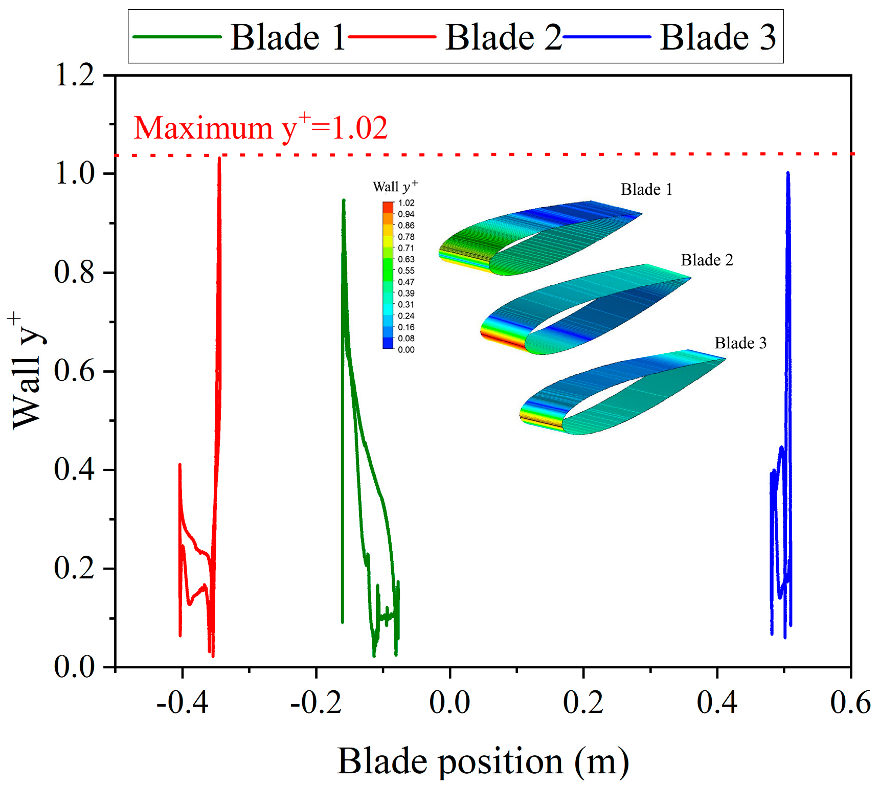
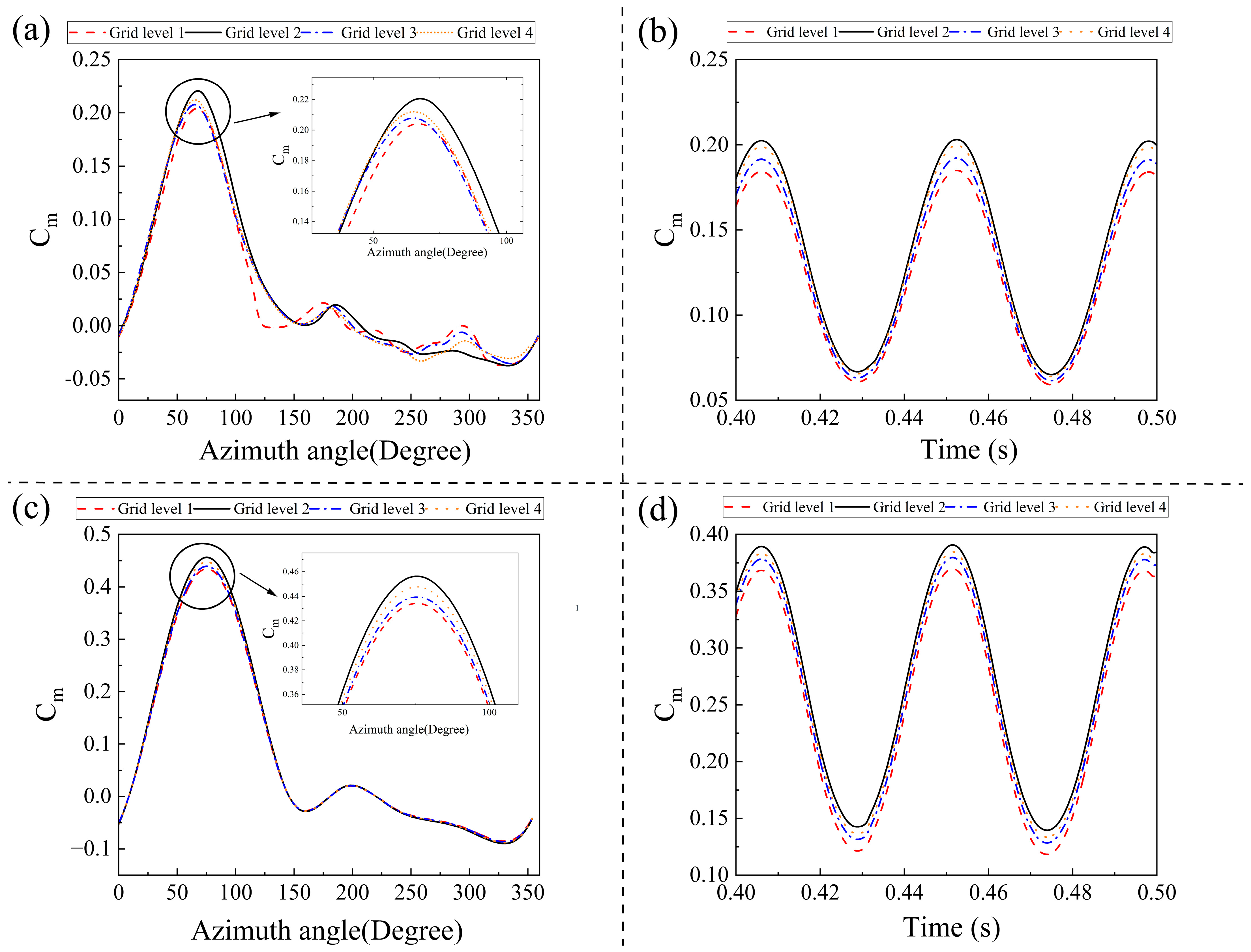
The current investigation uses Ansys Fluent 2021 R1 for numerical simulations. Due to the transient nature of the unsteady flow around the rotor blades, the transient method is the most suitable. We selected a pressure-based model suitable for incompressible air at low speeds to solve the momentum and continuity equations. The SIMPLE discretization method (Semi-Implicit Method for Pressure-Linked Equations) scheme is integrated for high precision, efficiently addressing velocity–pressure challenges by resolving the momentum and pressure correction equations separately. The SIMPLE algorithm’s effectiveness is improved using refined mesh quality and a small time-step size in the simulation. The second-order upwind method is used for discretizing equations related to pressure, momentum, turbulence kinetic energy, and specific dissipation rate, providing high accuracy and efficiency. This simulation monitors convergence via the torque coefficient ${ C}_m$, which is considered converged when the difference between consecutive periods is less than 1%. The convergence criteria for x- and y-velocity components, continuity, turbulence kinetic energy ($k$), and omega equations are set at a threshold of ${10}^{-6}$, with 30 iterations per time step to keep residuals below these limits. The emphasis is on ensuring that torque and power fluctuations display consistent trends before the turbine cycles can be deemed valid. Only after achieving this stability can the power be averaged to calculate $C_p$. Additionally, a rotor cycle is suitable for assessing torque on a single blade only after confirming the stabilization of oscillations.

3.7. Grid Study

Choosing the proper grid configuration for the current complex geometry is crucial for accurately capturing flow characteristics and fluctuations in proximity to the blade walls and in the meantime effectively reducing computational expenses. This CFD study used ANSYS-Mesh for both rotor and stator discretization. An appropriate size unstructured triangular grid is utilized for the computational domain, complemented by a quadrilateral inflation grid known as the boundary layer mesh. This mesh is specifically designed to enhance flow behavior in proximity to the blade walls, particularly at the leading and trailing edges of the blade tips, where the tangential velocity of the flow is significantly elevated. The implementation of this grid reduces flow discontinuities in these critical regions. Unstructured triangular grids were developed for both rotating and stationary zones. We implemented a strategy of gradual grid coarsening, which commences from the blade walls and continues toward the interface between the stator and rotor zones. This method allows for size variation across different regions, as finer grid sizes near the blades enhance accuracy, while the far-field zones do not require such precision; excessively fine grids in these areas only serve to escalate computational costs. The progressive increase in the size of the polyhedral triangular grids closely approximates the characteristics of prism grids. Furthermore, the gradual reduction in grid size contributes to solution accuracy, as abrupt variations in grid size can lead to solution divergence. This technique improves grid accuracy and quality by using inflation layers around the blade, eliminating sudden grid size changes around blade and rotating zones and ensuring smooth integration between the boundary layer prism grid and the triangular rotor grid. Each triangular element’s apex aligns with the prism grid’s edges. A non-conformal mesh with specific sizing enhances grid density and accuracy of flux calculations. The grid structure is shown in Figure 4.

Based on Figure 4a, the grid surrounding the airfoil profile was established with dimensions ranging from 0.05 mm to 0.1 mm, incorporating between 12 and 18 inflation layers and a growth rate varying from 1.2 to 1.05 for different grid levels for the Darrieus control case with the clean blade. Detailed specifications of the grid are provided in

Table 3. Grid independence summary [34].

Grid Properties	Grid 1	Grid 2	Grid 3	Grid 4
Number of elements $\times {10}^3$	441	564	786	846
Interface element size (mm)	10	8	6	4
Airfoil element size (mm)	0.05	0.03	0.015	0.01
Number of inflation layers	12	14	16	18
First layer thickness (mm)	0.029	0.024	0.019	0.014
Inflation growth rate	1.2	1.15	1.1	1.05
Maximum skewness	0.946	0.979	0.969	0.984
Averaged $y^{+}$	1.4	0.9	0.83	0.74
$C_p$	0.2918	0.2929	0.2939	0.2931

.

According to Table 3, Grid 1 represents the coarsest grid specification, while Grid 4 represents the finest. It is imperative to adhere to two grid quality criteria. The first indicator is skewness, which must remain below one for a triangular grid structure to ensure acceptable quality and to avoid divergence [35]. The second convergence criterion pertains to the averaged $y^{+}$, which is calculated based on the following [36]:

$$y^{+}={\displaystyle \frac{{\rho }_{\omega }y{u}_{\tau }}{{\mu }_{\omega }}}$$

(10)

where y represents the normal length between the center of the grid and the blade surface. ${\rho }_{\omega }$ and ${\mu }_{\omega }$ denote air density and dynamic viscosity near the blade surface, respectively.${ u}_t$ is defined as friction velocity and calculated as $\sqrt{{\displaystyle \frac{\tau }{\rho }}}$, where $\tau$ is considered as wall shear stress and is estimated by $\mu {\displaystyle \frac{\partial u}{\partial y}}.$ The fluid flow in the boundary layer is categorized into the laminar sublayer with a ${\mathrm{y}}^{+}$ range between 0 and 5, and the buffer layer with ${\mathrm{y}}^{+}$ range of 5 to 30. To accurately model the viscous sublayer for the $k-\omega$ turbulence model, $y^{+}$ value should be around one to ensure discretization accuracy [37]. According to Table 3, both the grid quality of skewness and the $y^{+}$ values fall within the acceptable range. Figure 5 presents the $y^{+}$ contour plot, reinforcing confidence in the grid’s quality.

According to Figure 5, which illustrates the wall y+ distribution along the clean blade in a spanwise direction after the initiation of rotation according to its projected position on the X-direction, the $y^{+}$ values for all blades remain consistently within the acceptable range of approximately one. Furthermore, the contour distribution of $y^{+}$ indicates that the peak $y^{+}$ value occurs at the blade’s leading edge, with the highest value recorded for blade 2.

Figure 6 illustrates the $C_m$ for a single blade throughout a complete rotation, along with the $C_m$ values constrained within a margin of 0.1 across various grid levels considering two different TSR values of 2 and 2.6 to examine grid convergence in both high and low TSR ranges. This representation demonstrates the results’ independence concerning the number and density of grids employed.

Based on Figure 6, it can be seen that variations in the density and number of elements for different grid levels did not have a significant effect on the $C_m$ of the rotor for both the single blade during a complete rotation and the total rotor $C_m$ within a one-second interval in both TSR = 2 and TSR = 2.6, which are considered to be in the low- and high-TSR ranges, respectively; they also exhibited similar behavioral trends. This finding highlights the results’ independence from the quantity and density of the grids utilized. About the $C_p$ values detailed in Table 3, Grid 3 achieved the highest $C_p$ value, in contrast, Grid 1 recorded the lowest. The variation between these two grid levels is minimal, measured at less than 1%, confirming the solution’s accuracy and independence from the number of elements.

3.8. Time Step Size Study

A key challenge in CFD projects is ensuring data stability at each time-step, especially for Darrieus VAWTs, which experience significant airflow fluctuations and higher vorticity gradient variability at low-TSR rates [38]. A time-step evaluation is applied to identify optimal time-step size for the Darrieus VAWT, leading to a refined selection for subsequent simulations that enhanced the results’ accuracy and reliability. The Courant–Friedrichs–Lewy ($\mathrm{C}\mathrm{F}\mathrm{L}$) criterion was applied to evaluate the time-step [39].

$$CFL={\displaystyle \frac{u·∆t}{∆x}}$$

(11)

Here, $\mathrm{u}$ represents the flow velocity around the airfoil, while $∆\mathrm{t}$ is the time-step and $∆\mathrm{x}$ is the distance between cell centers. The $\mathrm{C}\mathrm{F}\mathrm{L}$ number relates the time-step $∆\mathrm{t}$ to the time required for a fluid particle with velocity $\mathrm{u}$ to travel across a cell of size $∆\mathrm{x}$. Equation (12) expresses the relationship between the time-step and azimuth angle across different angular velocities.

$$∆t={\displaystyle \frac{∆\theta }{\Omega ·\frac{180}{\pi }}}$$

(12)

The above equation defines the relation between the azimuth angle and the time-step size. $∆\theta$ represents the variations in azimuth angle according to rotor rotation, while Ω denotes the angular velocity.

For viscous turbomachinery flows, it is advisable to maintain a Courant number of approximately 10 to minimize errors [39].

Table 4. $\mathrm{C}\mathrm{F}\mathrm{L}$ for various spatial and temporal discretization [34].

TSR	$\Omega$(rad/s)	$∆\mathit{\theta }\left(\mathit{d}\mathit{e}\mathit{g}\mathit{r}\mathit{e}\mathit{e}\right)$	$∆\mathit{t}\left(\mathit{s}\right)$	$∆\mathit{x}\left(\mathit{m}\mathit{m}\right)$
				2.5 Grid 1 $\mathit{C}\mathit{F}\mathit{L}$	2.1 Grid 2	1.7 Grid 3	1.3 Grid 4
2	35.4	2	0.001	34	39.6	48.4	61.7
		1	0.0005	17	19.8	24.2	30.8
		0.5	0.00025	8.9	9.9	12.1	15.4
		0.1	0.00005	1.7	2	2.4	3
3.3	57.3	2	0.0006	32.6	36.92	45.3	57.61
		1	0.0003	16.3	18.5	22.6	28.8
		0.5	0.00015	8.4	9.2	11.3	14.4
		0.1	0.00003	1.7	1.8	2.2	2.9

outlines the CFL values for various grid configurations and time-steps at two TSRs of 2 and 3.3. The differing time-step values result from specific assignments of $∆\theta$ for each angular velocity, as stated in Equation (12). These variations are anticipated not to impact the output data, such as $C_m,$ significantly. In addition, the CFL condition remaining within an acceptable range demonstrates the simulation’s independence from the time-step, thereby facilitating the selection of an optimal time-step.

According to Table 4, the time-steps of 0.00025 s and 0.00015 s correspond to TSRs of 2 and 3.3, respectively, which exhibit variations in the azimuth angle of 0.5°. These time-steps are deemed suitable as their Courant numbers fall within an acceptable range for grid levels 1 and 2. Furthermore, it is advisable to select grid level 2 due to its finer structure, which has been determined to be acceptable according to the grid study.

To demonstrate the results’ robustness and independence from time-step size, alongside the Courant number study and its placement within an acceptable range, the rotor’s $C_m$ at various time-steps and variations in azimuth angle, as outlined in Table 4, were examined, and the results are illustrated in Figure 7.

In Figure 7, the variations in $C_m$ exhibit a consistent pattern throughout different time-step sizes within different azimuth angle variations. Also, the change in average $C_m$ remains negligible across different time-steps, with a relative difference of merely 1% observed as the angle transitions from 0.1° to 1°.

Following the grid independence study, it was determined that the variations in $C_p$ were insignificant from grid level 2 onward. Consequently, this specific grid was selected for the grid structure in this CFD simulation. The CFD time-step size must be determined according to $∆\theta =0.5°$, which resulted in a CFL number of less than 10 for both TSR values. As a result, this particular time-step serves as the main time-step size to ensure the accuracy of the current simulations.

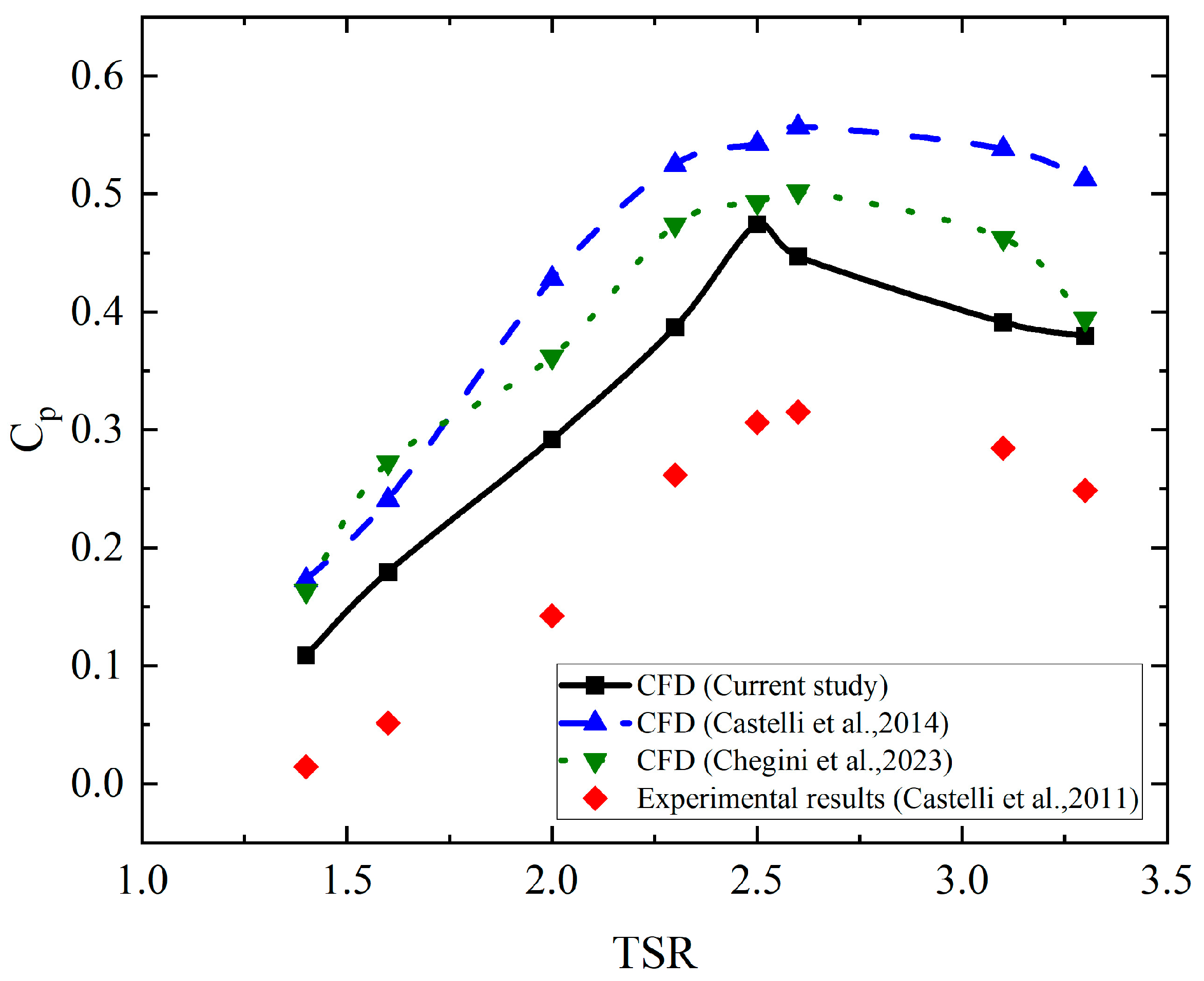
3.9. CFD Model Validation

CFD model verification was based on the model from Castelli et al. [40] as the control case, which contains both CFD and experimental findings. Previous extra CFD studies were included in order to robust validation process. The experimental study did not reference the blocking effect, resulting in its ignorance in current numerical simulations. V = 9 m/s ($\mathrm{R}\mathrm{e}=\mathrm{740,000}$) was employed as the inlet boundary condition, aligning with the wind tunnel conditions. Verification was conducted on $C_p$ calculation over eight TSRs between 1.4 and 3.3, as shown in Figure 8.

To validate the precision of our CFD findings, the current CFD results are compared with experimental wind tunnel data from Castelli et al. [40] and numerical data from Chegini et al. [41] and Castelli et al. [24]. Our CFD simulation demonstrated a noteworthy alignment with both experimental and prior CFD outcomes. Upon analysis, our findings were more consistent with real-world scenarios than the previous CFD findings. Specifically, at TSR = 2.5, our study yielded $C_p$ of 0.47, reflecting deviations of 4% and 15% from the earlier results of Chegini et al. [41] and Castelli et al. [24], respectively, thus indicating considerably closer agreement with experimental findings. The improved alignment of the current CFD results with the experimental control case can be attributed to more precise grid discretization and careful selection of the domain dimensions. These enhancements represent a significant advantage over the earlier CFD analyses. The observed discrepancy between the experimental data and both current and prior CFD results is due to several factors. These include the simplifications inherent in 2D solutions, the reliance on RANS models, and excluding losses associated with mechanical components such as arms, shafts, and bearings. Nevertheless, our recent CFD findings exhibit improved alignment with experimental data, which is credited to a refined grid structure and a robust domain dimensions sensitivity analysis. It is important to acknowledge that 2D-URANS approaches are generally preferred in various CFD modeling because of their cost-effectiveness. The minimal errors within these CFD models are often considered acceptable when weighed against their advantages regarding computational cost. Following 2D simulation was assumed on the rotor mid-plane, implying that a solo plane was examined through the central part, facilitated a segmented analysis of the turbine. Flow analysis was executed considering this mid-plane assumption, which yields satisfactory accuracy for vortex simulations. Specifically, these simulations focus on the mid-plane of the Darrieus VAWT, which is identified by a considerable blade aspect ratio (height-to-chord ratio) of 16.97, thereby excluding the influence of 3D tip vortex effects. According to Equation (5), which illustrates the calculation of $C_p$ from rotor power, the turbine power depends on the multiplication of rotor dynamic torque and angular velocity. Consequently, the valid results for $C_p$ can be applied to dynamic torque as well.

The CFD solution is considered valid, meeting benchmarks from the literature, grid verification, and time-step studies. It aligns with previous CFD trends and experimental results, demonstrating reliability.

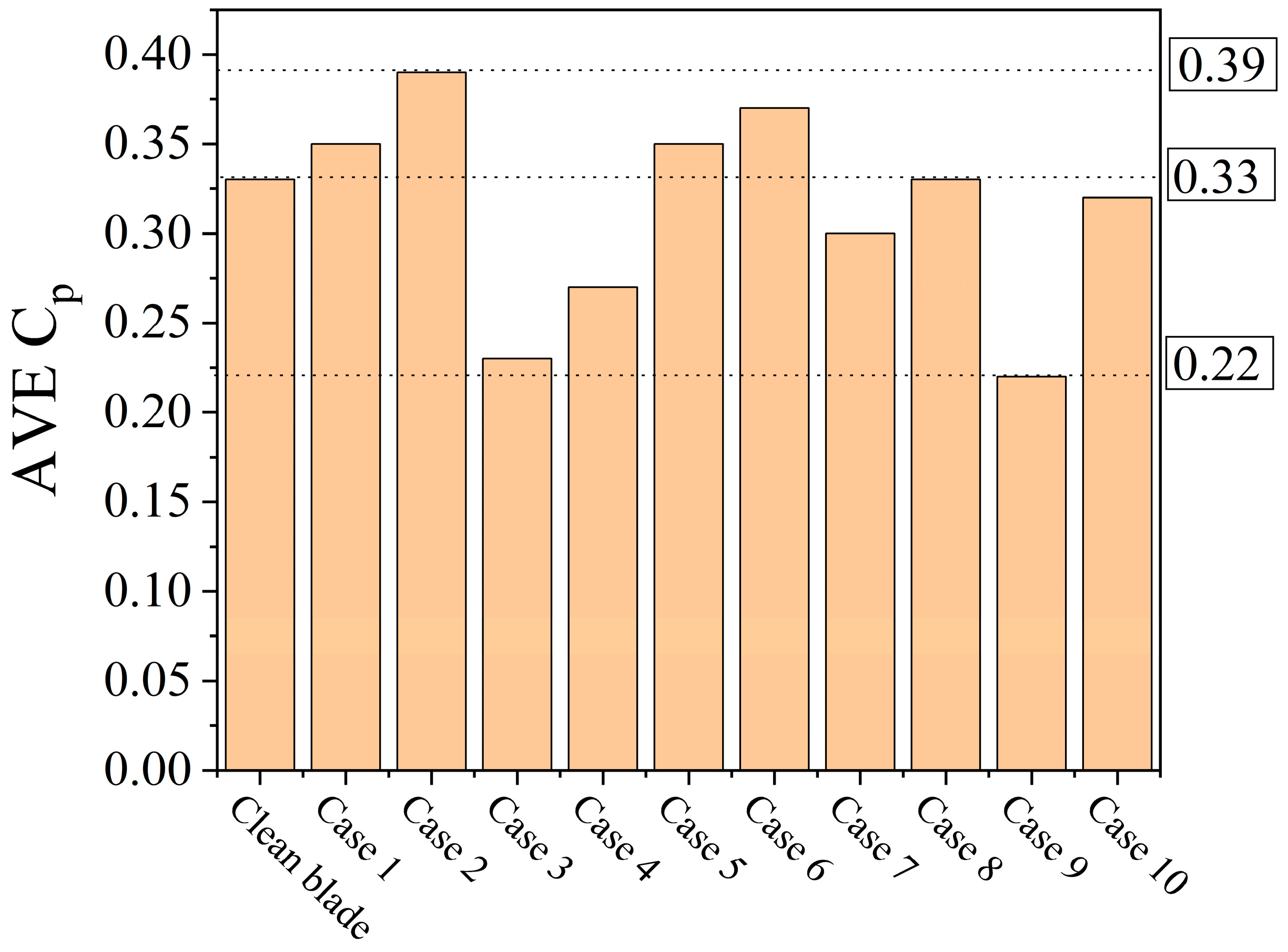
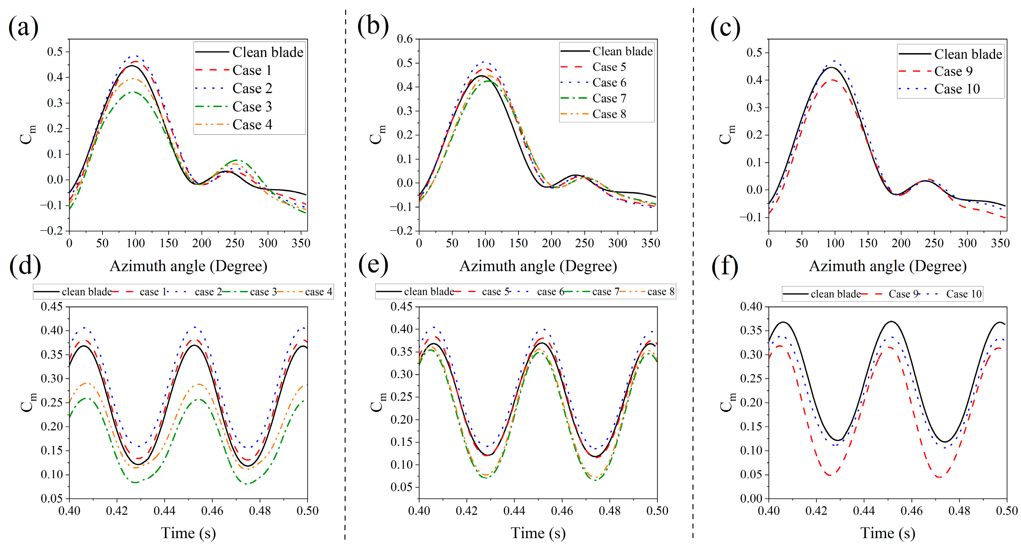
4. Results and Discussion

In this section, we analyze the effects of various KF airfoil profiles and configurations, including differences in step lengths and depths, as outlined in Table 2. This table outlines ten distinct configurations of KF blade profiles, specifying the sides, length, and the depth of the horizontal step. The impact of these configurations on the performance of the Darrieus rotor performance is evaluated by examining the rotor’s power efficiency and surrounding flow field. Figure 9 illustrates the assessment of rotor performance.

Figure 9a presents the power efficiency of KF blades with the step placed on the inner side of the airfoil. A notable increase in $C_p$ is observed in case 2, where the step features are minimized dimensions of 20%$c$ in length and 2%$c$ in depth. This configuration demonstrates enhanced performance compared to the rotor with a clean airfoil profile, particularly in the high-TSR range. It achieves its maximum performance at TSR = 2.5, surpassing the clean blade by 25%. Furthermore, case 1, which is defined by dimensions of 20%$c$ in length and 5%$c$ in depth, demonstrates enhanced performance compared to the clean blade configuration, particularly within the high-TSR range. However, it is noteworthy that its $C_p$ improvement at TSR = 2.5 was less significant than that in case 2, showing only a marginal enhancement of 9% compared to the clean blade configuration. In contrast, the KF blades with longer steps, as seen in cases 3 and 4, which both incorporate a length of 50%$c$ but with a depth of 10%$c$ and 5%$c$, respectively, demonstrate a significant decrease in $C_p$, compared to the clean blade across both high and low TSR ranges. Specifically, cases 3 and 4 showed significant $C_p$ reduction within TSR = 2.5 by 28% and 16%, highlighting the inefficiency of KF blades with longer steps. A similar behavior is observed in Figure 9b, where the steps are positioned on the blade’s outer side. Cases 5 and 6, which feature shorter step length, demonstrate superior performance compared to the clean blade. While case 5 shows only a marginal improvement in $C_p$ compared to the clean blade scenario, case 6 exhibits a significant enhancement of 25% in $C_p$, with TSR = 2.5. In contrast, case 7, which mirrors case 3 and possesses both the largest step length and depth, exhibits the most significant reduction in $C_p$ compared to other cases. Specifically, at TSR = 2.5, the $C_p$ reduces by 4%. This finding suggests that while case 7 decreased efficiency, the reduction in $C_p$ observed in this case is less pronounced than that in case 3. However, case 8, which mirrors case 4, shows marginal $C_p$ improvement in the high-TSR range. In summary, while positioning steps on the blade’s outer side enhances efficiency, the progress is less substantial than that on the inner side. Nonetheless, the efficiency reduction of KF blades with longer steps, specifically for cases 7 and 8, is less pronounced than that of cases 3 and 4. As illustrated in Figure 9c, which depicts KF blades with steps on both airfoil sides, case 9, featuring larger steps in both length and depth, experienced a notable reduction in $C_p$. In contrast, case 10, which incorporates shorter steps on both sides, improved $C_p$ within the high-TSR range compared to the clean blade.

Figure 10 displays the TSR-averaged $C_p$ for the 10 KF cases and the clean blade, visualizing each configuration’s overall performance.

According to Figure 10, the average $C_p$ of the rotors utilizing the KF airfoil demonstrates that case 2 achieves the highest average $C_p$ value, while case 9 yields the lowest average $C_p$value. Specifically, these values are 19% greater and 33% lower, respectively, compared to the control case with the clean blade. The figure also shows the inefficiency of steps with 50% chord length, regardless of whether positioned on the outer or inner sides, compared to the control case.

Figure 11a–c shows $C_m$ as a function of azimuth angle in a complete cycle for a single blade and Figure 11d–f shows $C_m$ variations over time.

Figure 11a–c demonstrates that $C_m$ of the single clean blade at the azimuth angle of 0° at the windward region is marginally greater than that of the KF blades. However, variations in $C_m$ across azimuth angles from 50° to 170°, with the rotor positioned within upwind and leeward, reveal that the $C_m$ values of the single KF blades are higher than those of the clean blade profile. In these specific positional instances, configurations featuring shorter step lengths of 20%$c$, irrespective of their placement on the outer or inner sides (notably cases 1, 2, 5, 6, and 10), exhibit higher $C_m$ values for single blade in comparison to cases utilizing a 50%$c$ step length. In the case of KF blades with 20%$c$, cases 2 and 6, which have a depth of 2%$c$, show a higher $C_m$ value, specifically at an azimuth angle of 100°. As the scenario involving a 50%$c$ demonstrates a lower $C_p$ value compared to the control case, it indicates diminished $C_m$ values relative to the control case within a complete rotation.

Figure 11d–f shows that the rotor $C_m$ aligns with the power efficiency curve. Notably, the rotor $C_m$ values for the configurations featuring the KF blade with 50%$c$ (cases 3, 4, 7, 8, and 9) are lower than the rotor $C_m$ of the control case, which uses a clean blade. Furthermore, the rotor $C_m$ for case 10, which exhibited a marginally lower $C_p$ at the TSR of 2.6—refer to Figure 9—marking the onset of the high-TSR range is also lower than the control case. However, cases 2 and 6, which have higher $C_p$ at TSR = 2.6, show higher $C_m$ values compared to other KF blades and the clean blade. Also, the configurations of the KF blades, particularly those with a 50%$c$, do not enhance the self-starting capability when compared to the control case, as their initial $C_m$ value is inferior to that observed during the two rotor periods and within the windward region. This observation highlights the pronounced necessity of KF blades (cases 3, 4, 7, 8, 9, and 10) for increased initial torque for successful start-up operation. This observation underscores that selecting the KF blade with long steps is not advisable for rotor blade design.

To enhance our understanding of rotor blade behavior, we presented the pressure field associated with KF blades in various positions and analyzed the best- and worst-case scenarios. Specifically, cases 2 and 3 illustrate conditions where the steps are positioned on the inner sides, while cases 6 and 7 address scenarios with steps located on the outer sides. Additionally, we examine KF blades featuring steps on both sides.

According to Figure 12, when the rotor is positioned in the windward section within azimuth angles ranging from 0° to 45°, the favorable positive pressure about 300 Pa on the leading edge facilitates rotor rotation, resulting in higher $C_m$ compared to the control case. The presence of negative pressure along the lower surface, near the leading edge, contributes favorably to blade rotation and increasing $C_m$. However, it is essential to acknowledge that a negative pressure zone develops toward the trailing edge when the KF blade incorporates 50%$c$ or 20%$c$ steps. This phenomenon is observable in both windward and upwind regions, spanning angles from 0° to 135°. Furthermore, due to the more pronounced negative pressure associated with the 20%$c$ configuration, there is a correspondingly enhanced positive effect on rotor rotation. Therefore, the development of a negative pressure zone on the inner side of the blade for case 2, which has a shorter step length, from the leading edge toward the trailing edge, observed in both the upwind and windward regions, resulted in an improvement in $C_m$, as confirmed by the findings presented in Figure 11d. When the rotor blade is positioned within the leeward section at azimuth angles of 180° and 225°, both configurations exhibit identical pressure field distributions, resulting in equivalent $C_m$ values. Furthermore, as the blade transitions to the downwind section at an azimuth angle of 270°, the negative pressure zone observed on the KF blade—particularly with 50%$c$ outer side proximity to the trailing edge—facilitates rotor rotation and yields marginally higher $C_m$ values.

According to Figure 13, the pressure field within the windward section at an azimuth angle of 0° is consistent. However, as the blade approaches the upwind section, although a favorable positive pressure gradient of 300 Pa is observed on the leading edge, a positive pressure zone around 200 Pa is observed on the trailing edge of the KF blade with a 50%$c$ step at azimuth angles ranging from 45° to 135°. This phenomenon interferes with the rotor rotation by inducing adverse pressure on the rotor blade in the opposite direction of its rotation. Consequently, this results in a decrease in the rotor’s $C_m$ when compared to the KF blade, which features a length of 20%$c$. However, the pressure distribution in the leeward and downward sections from 135° to 315° exhibits identical characteristics, particularly within an azimuth of 180°. This similarity results in comparable values of $C_m$.

According to Figure 14, when the blade is oriented at windward and upwind sections at azimuth angles of 40° and 90°, a positive pressure zone of 200 Pa is observed on the trailing edge of the KF blade with a 50%$c$ step. This condition is characterized as an unfavorable pressure gradient, analogous to what was observed in case 7, where a positive pressure value of approximately 200 Pa is exerted on the trailing edge tip. Additionally, when the horizontal slot step shape is elongated, the location of the positive pressure effect extends over a longer arm, resulting in an increased adverse torque that opposes the rotor’s rotation, which resulted in a reduction in the $C_m$ compared to the KF blade with a 20%$c$ step (refer to Figure 13). However, it is noteworthy that the pressure fields within the leeward and downwind sectors from 135° to 315° are almost identical, leading to comparable $C_m$ values between the azimuth angles of 135 and 270°. Additionally, the presence of a negative pressure zone on the outer side of the KF blade with a 20%$c$ step facilitates rotor rotation, resulting in a marginal improvement in the $C_m$ compared to the KF blade with a 50%$c$ step.

Figure 15 depicts $C_l$ as a function of AoA and azimuth angle, providing a deeper understanding of rotor’s aerodynamic performance.

Figure 15a–c depicts the KF blades featuring a 50%$c$ step, showcasing the inner side (cases 3 and 4), the outer side (cases 7 and 8), and both sides (case 9). These configurations demonstrate reduced $C_l$ when compared to the KF blades with shorter step lengths within an AoA range of 0° to 40° as they have lower $C_p$ and $C_m$ values too. Notably, case 3 achieves a peak $C_l$ of unity at an AoA of 30°, a value that is inferior to those observed in other configurations, thereby underscoring its suboptimal design for a Darrieus rotor application. Given that the principles governing Darrieus rotors rely fundamentally on lift force generation, the observed reduction in $C_l$ values across various blade positions indicates a decrease in rotor efficiency equipped with a KF blade with a longer step length. In contrast, cases 2 and 6, which incorporate a 20%$c$ step in length and 2%$c$ in depth, which is less than other KF blades, exhibit the highest values of $C_l$, indicating their superior performance compared to other configurations with KF blades. An analysis of cases 2 and 6, based on their $C_p$ (refer to Figure 10) and $C_m$ (refer to Figure 11), as well as their elevated $C_l$ values across the entire AoA range—culminating in peak $C_l$ values of 1.3 and 1.6 at an AoA of 30°, respectively—suggests that these configurations possess distinct advantages over other KF blade designs.

Figure 15d–f demonstrates that the KF blades with a 50%$c$ step length exhibits lower $C_l$ values, particularly within the azimuth angles ranging from 50° to 150°, in both the upwind and leeward configurations. Upon analysis of Figure 15a,d, it becomes apparent that when the step is positioned on the inner side specifically for cases 1 and 2 with 20%$c$ step length—taking into account the flow direction at an azimuth angle of 60° and AoA of 30° where the blade is located at the upwind region—an equivalent positive effective camber is achieved for the blade. As a result, this configuration yields positive $C_l$ values at an AoA of 30° in the upwind region compared to the clean blade. Therefore, the step configuration contributes to a positive equivalent camber for the KF blades, leading to an enhancement in $C_l$relative to the clean blade. In cases 3 and 4, implementing a 50%$c$ step length, despite adhering to the specified flow direction with an AoA of 30° and an azimuth angle of 60°, resulted in a positive equivalent camber and an increased $C_l$ compared to the control case. However, the extended step length and more depth values of 10%$c$ and 5%$c$ led to the presence of trapped swirling flow around the trailing edge, which induced flow separation and detachment, in contrast to the performance observed with the clean blade. In contrast, cases 1 and 2, which feature shorter step lengths and depth values, did not exhibit significant flow separation around the trailing edge, leading to an improvement in $C_l$ when compared to the control case. The observed reduction in $C_l$ for KF blades with extended step lengths, particularly in the context of case 3 at an azimuth angle of 60°, aligns with an AoA of 30°, which is markedly higher than the static stall angle; and also, the decline in $C_l$ noted within the azimuth angles ranging from 250° to 350° corresponds to AoA values between −10° and −30°, signifying the blade’s approach towards the negative static stall angle and its transition from the downwind to the windward section under a sharp AoA. This decrease in $C_l$ indicates a potential occurrence of dynamic stall in this scenario, especially in the case of a 50%$c$ step on the inner side.

To enhance comprehension, Figure 16 presents the velocity field surrounding the rotor blade when Blade 1 is positioned at an AoA of −20°, which corresponds to an azimuth angle of 325°.

According to Figure 16, the wake flow generated behind the rotors with KF blades with 50%$c$ is significantly more severe, as indicated by the stagnation zone. The intensified wake region, along with the associated increase in flow unsteadiness, contributes to higher pressure drag and escalated energy losses. The configuration incorporating a longer step length on the KF blade demonstrates reduced aerodynamic performance. This extended step length introduces a more pronounced geometric discontinuity, exacerbating flow separation near the trailing edge at sharp AoA values. Consequently, this flow separation delays the attachment of the flow at the trailing edge, particularly in regions with high-velocity areas around the steps. As a result, effective lift generation is diminished due to disrupted flow separation and delayed attachment. The flow separation and subsequent delay in flow reattachment for KF blades with a 50%$c$ not only resulted in blade instability but also contributed to rotor inefficiency. This inefficiency is the underlying reason for the observed reduction in $C_p$.

According to Figure 17, the flow fields surrounding the KF blades with extended step lengths exhibit intensified and more dispersed regions of opposing vorticity. Notably, significant vorticity shedding occurs near the trailing edge, adversely affecting aerodynamic performance due to unfavorable vortex dynamics in that region. Z-vorticity contours illustrate pronounced and chaotic vortex shedding, characterized by extensive alternating zones of positive (blue) and negative (red) vorticity. This observation suggests that KF blades with 50%$c$ experience delays and inefficiencies in effectively suppressing flow separation. Consequently, the flow at the trailing edge becomes highly unsteady, disrupting pressure recovery and delaying flow attachment, which diminishes lift force under sharp angles of attack, potentially leading to dynamic stall occurrences. The weakened and irregular vortex structures result in a decrease in time-averaged lift force and an increase in unsteady aerodynamic loading, significantly diminishing the turbine blade’s efficiency and stability. Consequently, blade instability and reduced lift force, the prevailing aerodynamic force that causes Darrieus rotor rotation, result in reduced extracted power ($C_p$) of the rotors with KF blades configuration with longer step length.

5. Conclusions

This study examines the impact of the KF blade airfoil profile on the aerodynamic performance of the Darrieus VAWT. Ten distinct airfoil profiles are analyzed, each featuring varying step lengths and depths of the KF blade steps. The step arrangements vary with placements on the inner side, the outer side, or both sides of the airfoil. The results indicate that KF airfoil with shorter step lengths and depth values, e.g., a step length of 20%$c$ and a depth of 2%$c$, can enhance $C_p$ in the high-TSR range. In contrast, KF blades with longer lengths and depth values, specifically those with 50%$c$ length and 10%$c$ depth, resulted in a reduction of $C_p$ values across both low- and high-TSR ranges when compared to the rotor with a clean blade. Additionally, it is noteworthy that KF blades with both side steps, when incorporating a step length of 50%$c$, significantly reduced the $C_p$ across all TSRs as well. Upon evaluating the average $C_p$ values across both low- and high-TSR ranges, it was observed that case 9, which features KF blades with extended steps on both sides, and case 2, characterized by shorter steps on the pressure side, were identified as the least favorable and optimal KF blade configurations, respectively, compared to the clean blade. The analysis of $C_m$ and $C_l$, in conjunction with observations of fluid flow physics, indicates that a positive unfavorable pressure gradient affects the KF blade trailing edge with longer steps when the blade is positioned in the upwind region. This condition leads to a reduction in $C_m$, which has adverse implications for aerodynamic efficiency in cases 3, 7, and 9 with 50%$c$ step. Additionally, blades exhibiting longer steps on the inner side experienced flow separation and delayed flow attachment on these extended step surfaces as considering flow direction and equivalent negative camber when positioned at high azimuth angles and sharp AoA values, resulting in a decrease in $C_l$ and an increase in the occurrence of dynamic stall as the $C_l$ value for the case 3 reduced to unity at AoA of 30° and azimuth angle 60°, which is lower than case 2. However locating the steps on the outer side and considering same azimuth angle and AoA, the positive equivalent camber results in $C_l$ increase for different KF blade configuration compared to the clean blade. Taken together, the KF blades reveal that those with longer lengths and deeper steps, specifically cases 3 and 7, with 50%$c$ in length and 10%$c$ in depth, as well as case 9, with 50%$c$ in length and a 5%$c$ in depth, are adversely affected by the unfavorable pressure value accumulated on their trailing edge tips, which resulted in $C_m$ reduction by imposing opposite torque. This condition, coupled with the negative impact of flow separation and severe blade instability, has reduced $C_l$ and inefficiency. This inefficiency is further highlighted by the diminished $C_p$ within almost all TSR ranges.

6. Further Study

Upon examining the $C_l$ and $C_m$ values, it is evident that they remain consistent across the initial azimuth angles for the KF blade compared to the clean blade. Additionally, the KF blade exhibits either identical or lower $C_p$ values compared to the clean blade within the low-TSR range, wherein the rotor initiates rotation. Consequently, although there were marginal improvements in the KF blades with 20%$c$ in length, we cannot anticipate that implementing the KF blade as a passive modification will enhance self-starting capability. The only improvement in $C_p$ occurs within the high-TSR range, indicating that it may be beneficial to explore flow control methods—such as the installation of guide vanes and other external objects—to enhance $C_p$ within the low-TSR range and improve self-starting capability. In applying the KF blade to the Darrieus rotor, particularly when both the step length and depth are substantial on both inner and outer sides, it is important to note that a reduction in blade thickness may adversely impact the blade’s structural integrity. Although the blade’s trailing edge in this study possesses an adequate thickness that meets satisfactory standards, this research primarily focuses on the aerodynamic performance and flow physics. Therefore, it is advisable to conduct a Fluid–Structure Interaction (FSI) study on the 50% chord KF blade configuration, specifically in windward and upwind positions where positive pressure is imposed on the tip of the trailing edge, to ensure the strength of the blade.

References

1. Holechek, J.L.; Geli, H.M.E.; Sawalhah, M.N.; Valdez, R. A Global Assessment: Can Renewable Energy Replace Fossil Fuels by 2050? Sustainability 2022, 14, 4792. [Google Scholar] [CrossRef]
2. Liu, S.; Zhang, L.; Lu, J.; Zhang, X.; Wang, K.; Gan, Z.; Liu, X.; Jing, Z.; Cui, X.; Wang, H. Advances in urban wind resource development and wind energy harvesters. Renew. Sustain. Energy Rev. 2025, 207, 114943. [Google Scholar] [CrossRef]
3. Shen, Z.; Gong, S.; Zuo, Z.; Chen, Y.; Guo, W. Darrieus vertical-axis wind turbine performance enhancement approach and optimized design: A review. Ocean. Eng. 2024, 311, 118965. [Google Scholar] [CrossRef]
4. Selvarajoo, S.R.; Mohamed-Kassim, Z. The effects of dynamic stalls on the aerodynamics and performance of a Darrieus rotor during self-start. Phys. Fluids 2024, 36, 015143. [Google Scholar] [CrossRef]
5. Redchyts, D.; Fernandez-Gamiz, U.; Tarasov, S.; Portal-Porras, K.; Tarasov, A.; Moiseienko, S. Comparison of aerodynamics of vertical-axis wind turbine with single and combine Darrieus and Savonius rotors. Results Eng. 2024, 24, 103202. [Google Scholar] [CrossRef]
6. Abdolahifar, A.; Zanj, A. A review of available solutions for enhancing aerodynamic performance in Darrieus vertical-axis wind turbines: A comparative discussion. Energy Convers. Manag. 2025, 327, 119575. [Google Scholar] [CrossRef]
7. Mohamed, O.S.; Ibrahim, A.A.; Etman, A.K.; Abdelfatah, A.A.; Elbaz, A.M.R. Numerical investigation of Darrieus wind turbine with slotted airfoil blades. Energy Convers. Manag. X 2020, 5, 100026. [Google Scholar] [CrossRef]
8. Acarer, S. Peak lift-to-drag ratio enhancement of the DU12W262 airfoil by passive flow control and its impact on horizontal and vertical axis wind turbines. Energy 2020, 201, 117659. [Google Scholar] [CrossRef]
9. Hosseini Rad, S.; Ghafoorian, F.; Taraghi, M.; Moghimi, M.; Ghoveisi Asl, F.; Mehrpooya, M. A systematic study on the aerodynamic performance enhancement in H-type Darrieus vertical axis wind turbines using vortex cavity layouts and deflectors. Phys. Fluids 2024, 36, 125170. [Google Scholar] [CrossRef]
10. Javaid, M.T.; Sajjad, U.; Saddam ul Hassan, S.; Nasir, S.; Shahid, M.U.; Ali, A.; Salamat, S. Power enhancement of vertical axis wind turbine using optimum trapped vortex cavity. Energy 2023, 278, 127808. [Google Scholar] [CrossRef]
11. Lee, K.-Y.; Cruden, A.; Ng, J.-H.; Wong, K.-H. Variable designs of vertical axis wind turbines—A review. Front. Energy Res. 2024, 12, 1437800. [Google Scholar] [CrossRef]
12. Farzadi, R.; Zanj, A.; Bazargan, M. Effect of baffles on efficiency of darrieus vertical axis wind turbines equipped with J-type blades. Energy 2024, 305, 132305. [Google Scholar] [CrossRef]
13. Naik, K.; Sahoo, N. Aerodynamic performance and starting torque enhancement of small-scale Darrieus type straight-bladed vertical axis wind turbines with J-shaped airfoil. J. Renew. Sustain. Energy 2024, 16, 033304. [Google Scholar] [CrossRef]
14. Zereg, A.; Aksas, M.; Bouzaher, M.T.; Laghrouche, S.; Lebaal, N. Efficiency Improvement of Darrieus Wind Turbine Using Oscillating Gurney Flap. Fluids 2024, 9, 150. [Google Scholar] [CrossRef]
15. Zhu, H.; Hao, W.; Li, C.; Luo, S.; Liu, Q.; Gao, C. Effect of geometric parameters of Gurney flap on performance enhancement of straight-bladed vertical axis wind turbine. Renew Energy 2021, 165, 464–480. [Google Scholar] [CrossRef]
16. Eltayeb, W.A.; Somlal, J. Performance enhancement of Darrieus wind turbines using Plain Flap and Gurney Flap configurations: A CFD analysis. Results Eng. 2024, 24, 103400. [Google Scholar] [CrossRef]
17. Chen, L.; Yang, P.; Zhang, B.; Chen, L. Aerodynamic Enhancement of Vertical-Axis Wind Turbines Using Plain and Serrated Gurney Flaps. Appl. Sci. 2023, 13, 12643. [Google Scholar] [CrossRef]
18. Syawitri, T.P.; Yao, Y.; Yao, J.; Chandra, B. Drag reduction of lift-type Vertical axis wind turbine with slit modified Gurney flap. J. Wind. Eng. Ind. Aerodyn. 2024, 253, 105853. [Google Scholar] [CrossRef]
19. Han, Z.; Chen, H.; Chen, Y.; Su, J.; Zhou, D.; Zhu, H.; Xia, T.; Tu, J. Aerodynamic performance optimization of vertical axis wind turbine with straight blades based on synergic control of pitch and flap. Sustain. Energy Technol. Assess. 2023, 57, 103250. [Google Scholar] [CrossRef]
20. Seyhan, M.; Akbıyık, H. An experimental investigation on the flow control of the partially stepped NACA0012 airfoil at low Reynolds numbers. Ocean. Eng. 2024, 306, 118068. [Google Scholar] [CrossRef]
21. Kabir, A.; Akib, Y.M.; Hasan, M.; Islam, M.J. Comparison of the aerodynamic performance of NACA 4415 and KFm based stepped airfoils. In AIP Conference Proceedings; AIP Publishing: Melville, NY, USA, 2021; Volume 2324. [Google Scholar]
22. Akbıyık, H. The effect of cavity modified stepped geometry on aerodynamic performance of an airfoil at a low Reynolds number. Phys. Fluids 2025, 37, 047106. [Google Scholar] [CrossRef]
23. Iddou, H.; Nait Bouda, N.; Benaissa, A.; Zereg, K. Numerical Analysis of the Kline and Fogleman Airfoil’s Effect on the Operation of Straight Darrieus Wind Turbine. J. Appl. Fluid Mech. 2024, 17, 1568–1592. [Google Scholar]
24. Castelli, M.R.; Englaro, A.; Benini, E. The Darrieus wind turbine: Proposal for a new performance prediction model based on CFD. Energy 2011, 36, 4919–4934. [Google Scholar] [CrossRef]
25. Sheidani, A.; Salavatidezfouli, S.; Stabile, G.; Rozza, G. Assessment of URANS and LES methods in predicting wake shed behind a vertical axis wind turbine. J. Wind Eng. Ind. Aerodyn. 2023, 232, 105285. [Google Scholar] [CrossRef]
26. Menter, F.R. Review of the shear-stress transport turbulence model experience from an industrial perspective. Int. J. Comput. Fluid Dyn. 2009, 23, 305–316. [Google Scholar] [CrossRef]
27. Meana-Fernández, A.; Fernández Oro, J.M.; Argüelles Díaz, K.M.; Velarde-Suárez, S. Turbulence-Model Comparison for Aerodynamic-Performance Prediction of a Typical Vertical-Axis Wind-Turbine Airfoil. Energies 2019, 12, 488. [Google Scholar] [CrossRef]
28. Spalart, P.; Allmaras, S. A one-equation turbulence model for aerodynamic flows. In Proceedings of the 30th Aerospace Sciences Meeting and Exhibit, Reno, NV, USA, 6–9 January 1992; p. 439. [Google Scholar]
29. Didane, D.H.; Rosly, N.; Zulkafli, M.F.; Shamsudin, S.S. Numerical investigation of a novel contra-rotating vertical axis wind turbine. Sustain. Energy Technol. Assess. 2019, 31, 43–53. [Google Scholar] [CrossRef]
30. Moghimi, M.; Motawej, H. Developed DMST model for performance analysis and parametric evaluation of Gorlov vertical axis wind turbines. Sustain. Energy Technol. Assess. 2020, 37, 100616. [Google Scholar] [CrossRef]
31. Bianchini, A.; Balduzzi, F.; Bachant, P.; Ferrara, G.; Ferrari, L. Effectiveness of two-dimensional CFD simulations for Darrieus VAWTs: A combined numerical and experimental assessment. Energy Convers. Manag. 2017, 136, 318–328. [Google Scholar] [CrossRef]
32. Rezaeiha, A.; Kalkman, I.; Blocken, B. Effect of pitch angle on power performance and aerodynamics of a vertical axis wind turbine. Appl. Energy 2017, 197, 132–150. [Google Scholar] [CrossRef]
33. Ghafoorian, F.; Enayati, E.; Mirmotahari, S.R.; Wan, H. Self-Starting Improvement and Performance Enhancement in Darrieus VAWTs Using Auxiliary Blades and Deflectors. Machines 2024, 12, 806. [Google Scholar] [CrossRef]
34. Ghafoorian, F.; Hosseini Rad, S.; Moghimi, M. Enhancing Self-Starting Capability and Efficiency of Hybrid Darrieus–Savonius Vertical Axis Wind Turbines with a Dual-Shaft Configuration. Machines 2025, 13, 87. [Google Scholar] [CrossRef]
35. Harris, M.J. Flow feature aligned mesh generation and adaptation. Ph.D. Thesis, University of Sheffield, Sheffield, UK, 2013. [Google Scholar]
36. Lositaño, I.C.M.; Danao, L.A.M. Steady wind performance of a 5 kW three-bladed H-rotor Darrieus Vertical Axis Wind Turbine (VAWT) with cambered tubercle leading edge (TLE) blades. Energy 2019, 175, 278–291. [Google Scholar] [CrossRef]
37. Marsh, P.; Ranmuthugala, D.; Penesis, I.; Thomas, G. The influence of turbulence model and two and three-dimensional domain selection on the simulated performance characteristics of vertical axis tidal turbines. Renew. Energy 2017, 105, 106–116. [Google Scholar] [CrossRef]
38. Balduzzi, F.; Bianchini, A.; Ferrara, G.; Ferrari, L. Dimensionless numbers for the assessment of mesh and timestep requirements in CFD simulations of Darrieus wind turbines. Energy 2016, 97, 246–261. [Google Scholar] [CrossRef]
39. Trivellato, F.; Castelli, M.R. On the Courant–Friedrichs–Lewy criterion of rotating grids in 2D vertical-axis wind turbine analysis. Renew. Energy 2014, 62, 53–62. [Google Scholar] [CrossRef]
40. Raciti Castelli, M.; Ardizzon, G.; Battisti, L.; Benini, E.; Pavesi, G. Modeling Strategy and Numerical Validation for a Darrieus Vertical Axis Micro-Wind Turbine. In Proceedings of the IMECE2010, Vancouver, BC, Canada, 12–18 November 2010; Volume 7: Fluid Flow, Heat Transfer and Thermal Systems, Parts A and B, pp. 409–418. [Google Scholar]
41. Chegini, S.; Asadbeigi, M.; Ghafoorian, F.; Mehrpooya, M. An investigation into the self-starting of darrieus-savonius hybrid wind turbine and performance enhancement through innovative deflectors: A CFD approach. Ocean. Eng. 2023, 287, 115910. [Google Scholar] [CrossRef]
Figure 1. (a) Computational domain and boundary conditions; (b) rotor with KF blades; (c) different KF blade airfoil profiles.
Energies 18 02718 g001
Figure 2. (a) Theoretical AoA variation with azimuth angle for different TSR, (b) partitioning of rotor trajectory, and (c) lift force and velocities on a blade.
Energies 18 02718 g002
Figure 3. Computational domain sensitivity analysis: (a) inlet distance effect, (b) outlet distance effect, and (c) domain width effect.
Energies 18 02718 g003
Figure 4. Grid configurations (a) control case grid with grid levels for clean blade [33] (b) different KF blade grid configurations (c) grid around the steps of the KF blades.
Energies 18 02718 g004
Figure 5. Wall y + on clean blade spanwise and contour plot [33].
Energies 18 02718 g005
Figure 6. (a) Single blade C m as a function of the azimuth angle in a complete rotation, (b) rotor C m variations with time in TSR = 2, (c) single blade C m as a function of the azimuth angle in a complete rotation, and (d) rotor C m variations with time in TSR = 2.6.
Energies 18 02718 g006
Figure 7. (a) Variation of C m in relation to time for different time-steps, and (b) time-step sensitivity analysis.
Energies 18 02718 g007
Figure 8. Comparison of C p from the present 2D simulation with experimental and CFD results [24,34,40,41].
Energies 18 02718 g008
Figure 9. Power efficiency of Darrieus VAWT with different KF airfoil.
Energies 18 02718 g009
Figure 10. TSR-Averaged C p for KF configurations and the clean blade.
Energies 18 02718 g010
Figure 11. (ac) C m variations as a function of azimuth angle, and (df) C m variations as a function of time at TSR = 2.6.
Energies 18 02718 g011
Figure 12. Pressure field for KF blades with steps on the inner side (a) case 2, and (b) case 3.
Energies 18 02718 g012
Figure 13. Pressure field for KF blades with steps on the outer side (a) case 6, and (b) case 7.
Energies 18 02718 g013
Figure 14. Pressure field for KF blades with steps on both sides (a) case 10, and (b) case 9.
Energies 18 02718 g014
Figure 15. (ac) C l variations as a function of AoA, and (df) C l variations as a function of azimuth angle at TSR = 2.6.
Energies 18 02718 g015
Figure 16. Velocity field for rotor blade at AoA = −20°, azimuth angle = 325°, and TSR = 2.6 in (a) case 2, (b) case 3, (c) case 6, (d) case 7, (e) case 10, and (f) case 9.
Energies 18 02718 g016
Figure 17. Vorticity field for rotor blade at AoA = −20°, azimuth angle = 325° and TSR = 2.6 in (a) case 2, (b) case 3, (c) case 6, (d) case 7, (e) case 10, and (f) case 9.
Energies 18 02718 g017