Flue Gas Temperature Distribution as a Function of Air Management in a High-Temperature Biomass Burner

Abstract

Nowadays, as a result of the increasing awareness of European societies and new legal regulations, the role of renewable energy sources in individual heating is growing. One of the forms of renewable heat and electricity production is the use of biomass pellet burners coupled with Stirling engines. To ensure high system efficiency, the combustion process of this type of fuel requires an appropriate design of the burners, which can provide high-temperature flue gases. This requirement may be challenging, as the long operation of such a burner may cause the thermal degradation of its components, mainly the upper burner wall. The subject of this analysis was a burner with a nominal power of 10 kW. As the analysis tool, a previously validated CFD model was used. In this work, two ways of thermal degradation prevention are presented. The first one is geometry optimization via secondary air hole distribution. The results show that an appropriate geometrical design of the burner may be an efficient way of shifting the high-temperature zone to the burner axis, which may mitigate the thermal degradation risk. Secondly, the inlet air mass flow is changed to show its impact on the presence and location of the high-temperature zone. Both methods can be treated as interesting ways for solving the challenge of the long-term operation of high-temperature biomass burners by avoiding thermal degradation.

1. Introduction

Current energy policies support green energy transformation, forcing distributed renewable energy sources to be developed. The domestic use of biomass has great potential to be used as one of such sources [1]. Solid biomass consumption for electricity generation has grown over the last 25 years, from 99 TWh globally in 2000 to 471 TWh in 2020 [2]. In 2020, the share of solid biomass in total electricity production from biomass was nearly 70%. At the close of 2020, the total capacity of renewable energy sources (RESs) in Poland reached 9979.2 MW, and biomass-based installations accounted for 1512.9 MW [3].

Biomass plays a key role in renewable heating sources in Poland [4]. A significant increase in biomass utilization in this sector is also evident. For example, in 2022, the share of solid biomass in district heat production in Poland amounted to approximately 13%. Analyses of the demand for pellets, one of the primary biomass fuels, indicate a further significant increase in demand in the coming years [5]. This is partly due to the rapid growth in the number of installed boilers using this fuel in decentralized heating systems (approximately 500,000 units in Poland). At the same time, efforts are being made to improve the efficiency of biomass use in individual heating systems.

One example is a biomass micro-cogeneration system based on a Stirling engine, capable of generating heat and electricity from solid biomass for individual use [6]. Integrating a combustion system with this type of engine imposes specific requirements on combustion. To maintain adequate power and efficiency, the combustion process must be conducted at as high a temperature as possible. Research has shown that when a Stirling engine is powered by exhaust gases, an exhaust gas temperature above 1100 °C is necessary for the system to function efficiently.

Achieving such high temperatures in a small, grate-fired biomass burner (with a power output of around 10 kW) is a considerable challenge. Standard burners in this power class, used in pellet boilers, generate exhaust gases at around 800–900 °C, which is sufficient for efficient boiler operation. Reaching the required high exhaust gas temperature requires, among other things, a low excess air ratio and the preheating of combustion air. This also creates several design and operational challenges for the burner. High combustion temperatures promote excessive nitrogen oxide (NOx) emissions [7]. Furthermore, since a large part of the combustion process in grate-fired pellet burners takes place within the burner’s geometry, operating under these high-temperature conditions increases the risk of the local burner overheating.

The literature contains numerous modeling analyses and experimental studies on small and medium-sized biomass burners. There are also a few studies related to biomass systems utilizing Stirling engines. Some of these systems achieve even higher combustion temperatures than specified. However, they are not grate-fired burners capable of the high-temperature combustion of unprocessed solid biomass.

Flame temperature measurements during biomass pellet combustion are described in [8]. The authors considered biomass pellets from pine wood, rice straw, and corn stalks. The maximum temperature reached 1600 °C. A similar study is presented in [9], although the study covers a higher range of operational parameters. The typical temperatures there oscillate around 1000–1600 °C.

The design of a premixed burner for gasified biomass combustion is described in [10]. The considered power range was 20–46 kW. The maximum temperature reached 1000 °C. The temperatures obtained by the premixed burners were reported to be 30% higher compared to non-premixed, conventional ones.

A biomass burner for sugarcane bagasse combustion was analyzed by [11]. The power of this burner was 360 kW. The numerical analysis of a small biomass burner is shown in [12]. The temperature reached in the described burner was 1050 K. The combustion process of torrefied and water-washed biomass is described in [13]. It was performed in a homemade, kg scale cylinder burner. The study focused on the impact of its parameters on emissions (SO₂, NO_x, PM).

A grate biomass burner equipped with a screw conveyor is shown in [14]. The authors aimed at high-temperature degradation prevention by designing a ventilation system which allowed the front side of the burner to be kept at a temperature below 350 °C.

Examples of biomass combined heat and power (bio-CHP) installations can also be found in the literature. An example of a 40 kW/0.5 kW pilot plant is described in [15]. Pine wood pellets were burned in a fluidized bed in a test rig. The flue gas temperature obtained varied from 800 °C up to nearly 900 °C. The electricity generation efficiency, referred to as the chemical energy of fuel, was 3.8%.

Another micro-scale micro-CHP is described in [16]. The installation was based on a fluidized bed Stirling engine operated using helium. The fuel used in the study was wood pellets. The installation had a power of 45 kWth and 5 kWe. A long-term lab test lasting 72 h revealed an electrical efficiency of 13–15%, although the system was operated at relatively low temperatures (610–640 °C for 35 kW).

The authors of [17] presented a 0.5 kWe Stirling engine connected with a two-stage vortex combustion chamber. The average gas temperature at the hot side of the heat exchanger was 1150 °C, while the heat exchanger’s external surface temperature was 810 °C. The obtained efficiency of the Stirling engine was 14.8%, while CHP efficiency was 65%.

The aim of this work is to develop a biomass burner on a several kW scale coupled with a Stirling engine. To allow for effective electricity production, the biomass should be burned in a relatively small but high-temperature burner, as the electricity production efficiency of Stirling engines is highly dependent on the temperature [18,19]. Another aim of this study is to make the solution operable with unprocessed biomass, to make its application broader. The solution should be accessible, so it should be relatively cheap; that is why the usage of very advanced materials is not recommended. It should fulfill the following requirements:

• Low emissions of gaseous pollutants (CO, NOx);
• A sufficiently high flue gas temperature (minimum 1000 °C) to ensure proper heat transfer from the flue gases to the surface of the hot head of the Stirling engine (adequate heat flux density);
• Minimal variability in the flow rate and temperature of the flue gases exiting the burner;
• Unprocessed or minimally processed biomass as the fuel;
• Long operation time (degradation prevention).

Meeting the above conditions is a significant challenge. As indicated earlier and in the authors’ previous work [20], one of the long-term challenges is the thermal degradation of the burner’s upper wall. The aim of this study is to find a solution to this problem by examining the geometry and operational conditions of the burner. To achieve this, a CFD model, verified in the previous work described in [20], was used.

The innovations of this study include the following:

• The development of a new biomass burner capable of achieving high flue gas temperatures (≥1000 °C) and suitable for coupling with micro-CHP systems based on Stirling engines;
• The use of a novel air supply system that enables both the preheating of combustion air and the partial cooling of the burner structure, thereby improving thermal efficiency and operational durability;
• The application of CFD modeling, validated in previous studies, to optimize the geometry and operational conditions of the burner for enhanced durability and minimized emissions.

The conditions enumerated above make the task challenging. As indicated above and in the authors’ previous work [20], the zone most prone to thermal degradation is the burner’s upper wall, which was confirmed in the pre-tests. The aim of this study is to find a solution to this problem by changing the geometry and/or operational conditions. For this purpose, a CFD model verified in the framework of the previous study described in [20], was used.

2. Methods: Mathematical Modeling

The biomass burner model constructed uses a simplified geometry, an example of which is shown in Figure 1. The basic elements of the model geometry are a steel tube with holes, a fuel bed, an outer pipe, an air inlet, and a flue gas outlet. The combustion process takes place in a tube of a smaller diameter, where a biomass bed is located in the lower section. Combustion air is supplied through an inlet positioned in the upper part of a surrounding tube of a larger diameter. Its topmost position is motivated by the installation constraints of the burner on the test stand and by air preheating/burner cooling. The air is preheated as it flows downward through this outer tube and is subsequently delivered to the combustion chamber (the smaller-diameter tube) via openings (diameter of 5 mm each) located at the bottom (primary air). The hot flue gases exit the burner through an outlet (Figure 1). The diameter of the smaller tube (the combustion chamber) is 96 mm (inner), with a 2 mm wall, and its length is 305 mm. The diameter of the outer, larger tube is 150 mm.

One of the main challenges in the numerical modeling of a biomass burner lies in the relatively complex thermal and flow phenomena occurring within the system. These processes require a comprehensive modeling of fluid dynamics coupled with chemical reactions and heat transfer. An additional major challenge is the modeling of the behavior of the solid fuel within the burner and its interactions with the gaseous phase present in the combustion chamber. The combustion of biomass fuel can be divided into three primary stages: moisture evaporation, devolatilization and combustion of volatile compounds, and combustion of solid residues (primarily carbon) [21,22]. Each of these stages involves mass loss and energy exchange with the surroundings. The first stage—moisture evaporation—involves the removal of water content from the fuel. This phase typically lasts from a few to several dozen seconds, depending on the prevailing temperature. This process is associated with minor mass and volume reduction, as the pellets are expected to have a relatively low moisture content (e.g., 6.82% [23], 7–12.5% [24]). The second stage involves the release of volatile combustible components. During this phase, a significant reduction in fuel bed mass and volume occurs, as volatiles generally constitute the majority of the biomass fuel (74–80% [25]). The fuel absorbs heat from the surroundings to facilitate the release of volatile species, which include hydrogen, carbon monoxide and dioxide, hydrocarbons, impurities such as ammonia or its derivatives, and, in some cases, sulfur compounds [26]. These volatiles subsequently undergo combustion within the burner chamber. The final stage is the combustion of the remaining carbon in the fuel. The amount of fixed carbon depends on the type of biomass and may range from a few to over 20% (e.g., 16–20.5% [25]). Regardless of the specific conditions, this is typically the longest-lasting stage of combustion. It results in the formation of CO₂ and CO, which, under appropriate process conditions, can further oxidize to CO₂ [26].

The mathematical model was created assuming that the fuel bed is a porous body with three zones in which the release of components, combustion, and the release and absorption of energy are realized. Air is supplied to the fuel bed through openings in the inner pipe, providing oxygen for combustion. The outer burner pipe of the selected design alternatives was covered with insulation consisting of a mineral wool layer and a sheet metal jacket to reduce heat loss by radiation. The insulation was applied in the model as a boundary condition of the outer pipe wall. The main boundary conditions are summarized in

Table 1. Boundary conditions.

Location	Conditions
Inlet	mass flow inlet, air, 25.3 kg/h, 373 K
Outlet	pressure outlet, opaque; external black body temperature: 623 K; internal emissivity: 1
Outer walls	thermal conditions: mixed; heat transfer coefficient: 8 W/m2K; free stream temperature: 300 K; external emissivity: 0.05; external radiation temperature: 300 K; shell construction: two layers: steel, 0.0025 m; mineral wool, 0.03 m; internal emissivity: 1; opaque
Internal pipe wall	thermal conditions—coupled; opaque; internal emissivity: 1; steel

. Reference [20] provides a detailed model description and presents a biomass burner model without insulation. The mathematical model was implemented in Ansys Fluent 2024 R1, Research License. The mesh was nearly 5,000,000 elements and approximately 900,000 nodes. The mesh validation covered an examination of 4 grids from approximately 1,200,000 up to 6,000,000 elements [20].

The mathematical model was built with numerical fluid mechanics tools based on the conservation equations of mass (Equation (2)), momentum (Equation (1)), and energy (Equation (3)). Due to the changing chemical composition of the fluid in the computational domain, the species conservation equation (Equation (4)) was also used [27].

$$S_{Tj},𝛻·\left(\rho \overrightarrow{u}\overrightarrow{u}\right)=-𝛻p+𝛻·\left(\stackrel{-}{\tau }\right)+\rho \overrightarrow{g}+\overrightarrow{F},$$

(1)

$$𝛻·\left(\rho \overrightarrow{u}\right)=S_{\mathrm{m}},$$

(2)

$$𝛻·\left(\overrightarrow{u}\left[\rho E+P\right]\right)=𝛻·[{\lambda }_{eff}𝛻T+\left(\stackrel{-}{\tau }·\overrightarrow{u}\right)]+S_g,$$

(3)

$$𝛻·\left(\rho \overrightarrow{u}{Y}_k\right)=-𝛻·\overrightarrow{J_k}+\dot{{\omega }_k}+S_k,$$

(4)

The following source terms were applied in the equations: $F$—force source term (including contributions from the porous bed); $S_k$—species generation rate in predefined sources; $S_g$—energy source term (also including contributions from the porous bed); and ${\omega }_k$—net rate of production of species $k$ due to chemical reactions. A standard k-epsilon turbulence model was applied to the model, with wall functions developed from [28]. The choice of the turbulence model was motivated by the fact that there are areas of gas rotation and recirculation in the domain, and the velocities in the domain are relatively low. The k-epsilon model has been used in other biomass combustion CFD models, e.g., [29] and [30]. The radiation model implemented in the computational domain is the Discrete Ordinates model. A conservative variant of the DO model with an extension to an unstructured grid was used [31]. Due to the presence of triatomic gases in the computational domain, the weighted-sum-of-gray-gases model (WSGGM) [32] was used to calculate the absorption coefficient.

The fuel bed model was implemented as a 3-zone porous body in which combustion reactions and the release/absorption of heat and species take place. The zones represent volumes of real biomass combustion processes [33]. The porosity of the bed was assumed to be 0.5 (in all porous zones) based on the experimental data shown in [34]. Viscous resistance was set as 211,100,000 1/m² in all directions. In zone one, fuel heating occurs (heat consumption), and the water contained in the fuel evaporates. The amount of heat absorbed in zone one was calculated as the heat needed to heat the fuel from ambient temperature to 100 °C and the heat needed to evaporate the water. The amount of water evaporated was calculated based on the biomass moisture content. The complete evaporation of the water contained in the fuel was assumed.

In zone two, further fuel heating and the release of volatile components take place. The volatile fraction composition was based on [35] and was confronted with the measured chemical composition and calorific value of the biomass. The fuel composition adopted for the calculation is 8.2% H₂O, 0.5% ash, 78.48% volatilities, 12.82% fixed carbon, 50.16% carbon, and 6.04% hydrogen. The composition of volatile components was assumed to be 60.11% carbon dioxide, 22.33% methane, 8.93% benzene, 7.82% carbon oxide, 0.56% hydrogen, and 0.25% ammonia.

The biomass has a lower heating value of 17.043 MJ/kg. In the third zone, there is a further supply of heat to the bed, a release of CO and CO₂, and heat generation from the oxidation of fixed carbon in the fuel. The total energy change in zone three is due to the difference in the amount of energy used to heat the bed and the energy from coal oxidation. A summary of the species released in the respective zones of the porous medium, as well as the corresponding energy flow, is as follows:

First zone:

• Release of H₂O;
• Consumption of energy.

Second Zone:

• Release of CH₄;
• Release of CO₂;
• Release of CO;
• Release of C₆H₆;
• Release of H₂;
• Consumption of energy.

Third zone:

• Release of CO₂;
• Release of CO;
• Consumption of O₂;
• Consumption of energy.

The Eddy Dissipation model was used to model the chemical reaction of combustion in the domain. This model avoids the need for computationally expensive chemical kinetics calculations based on the Arrhenius approach. The species undergoing combustion are $C_6{H}_6$, $C{H}_4$, $H_2$, and $CO$. In the species conservation equation (Equation (4)), the species production rate resulting from chemical reactions is defined as the minimum value obtained from the equations (Equations (5) and (6)):

$${\omega }_{k,r}^{\dot{}}=\left({\nu }_{k,r}^{″}-{\nu }_{k,r}^{\prime }\right)M_{w,k}A\rho \frac{\epsilon }{k_n}mi{n}_R\left(\frac{Y_R}{{\nu }_{R,r}^{\prime }{M}_{w,R}}\right),$$

(5)

$${\omega }_{k,r}^{\dot{}}=\left({\nu }_{k,r}^{″}-{\nu }_{k,r}^{\prime }\right)M_{w,k}AB\rho \frac{\epsilon }{k_n}\frac{{\sum }_P{Y}_P}{{\sum }_l^N{\nu }_{l,r}^{″}{M}_{w,l}},$$

(6)

The model also uses the formation of nitrogen oxides through three mechanisms: a thermal, prompt, and fuel mechanism.

3. Results

The burner presented in [20] (geometry I) was constructed and operated in real conditions. After 50 h of full-load operation, upper wall degradation was observed. The impact of the high-temperature zone on the internal wall was identified as the main cause of this problem. CDF modeling results confirmed the presence of a high-temperature flue gas stream in the neighborhood of the damaged zone (Figure 2, steady-state simulation). The analysis presented in this study aimed at optimizing the geometry and operational parameters to fulfill the assumed requirements of the high-temperature burner (mainly maintaining the temperature of the flue gases at the outlet higher than 1000 °C) and to limit the risk of wall degradation due to temperature. 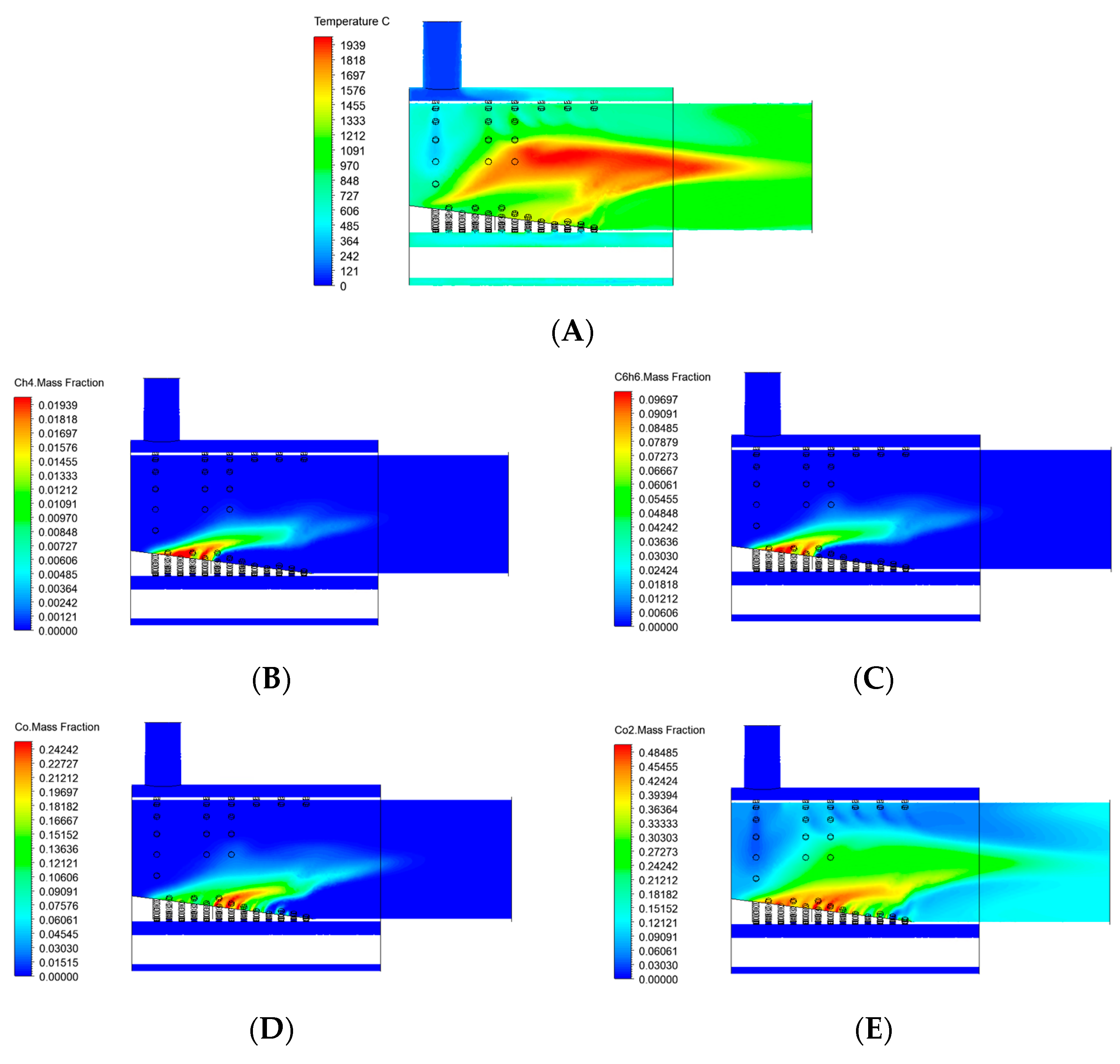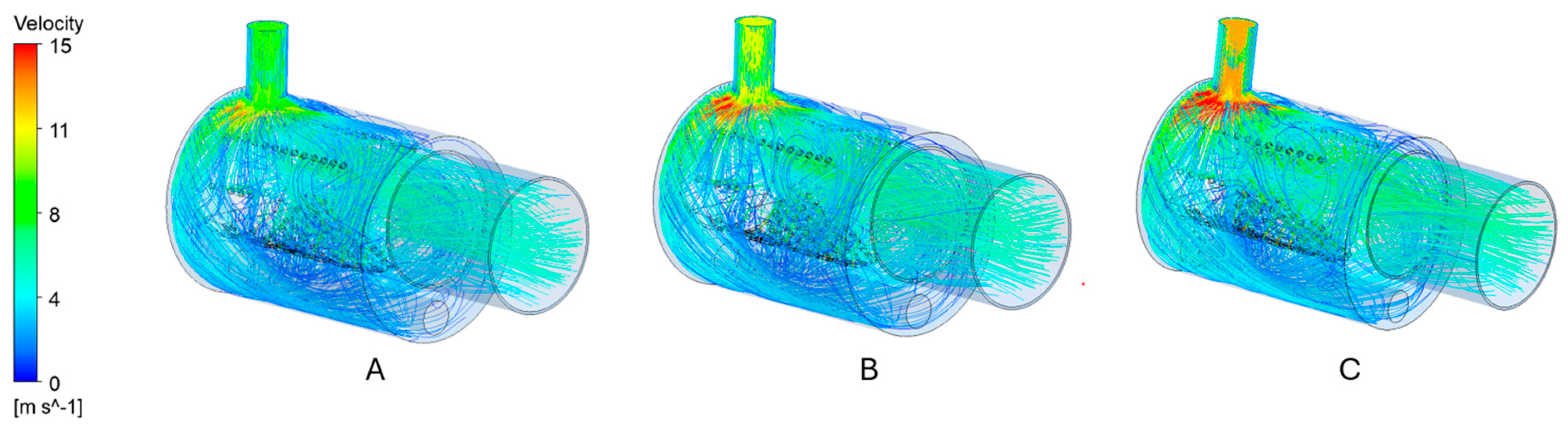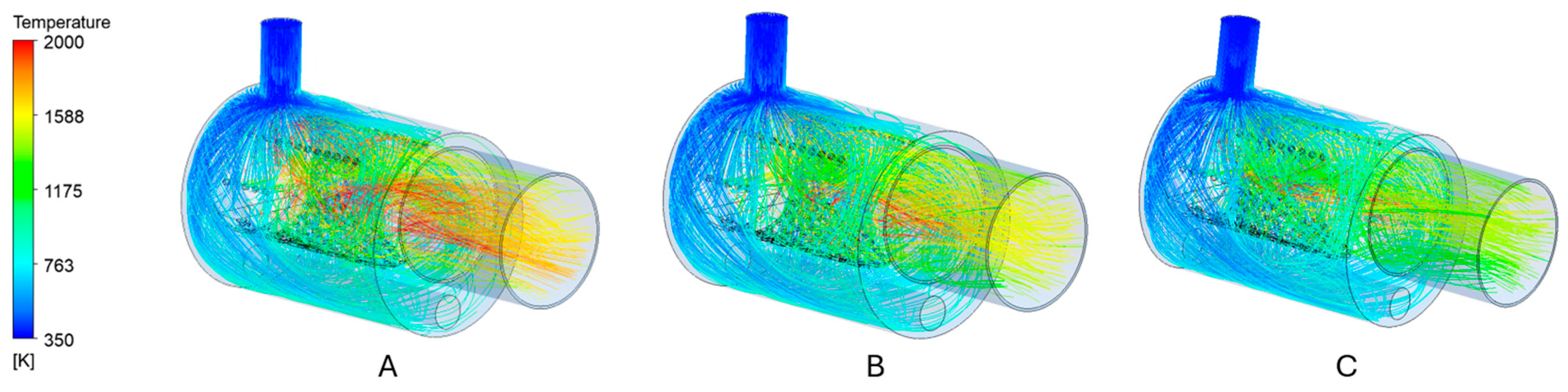The analysis was divided into two sections: geometry optimization and air mass flow rate tests.

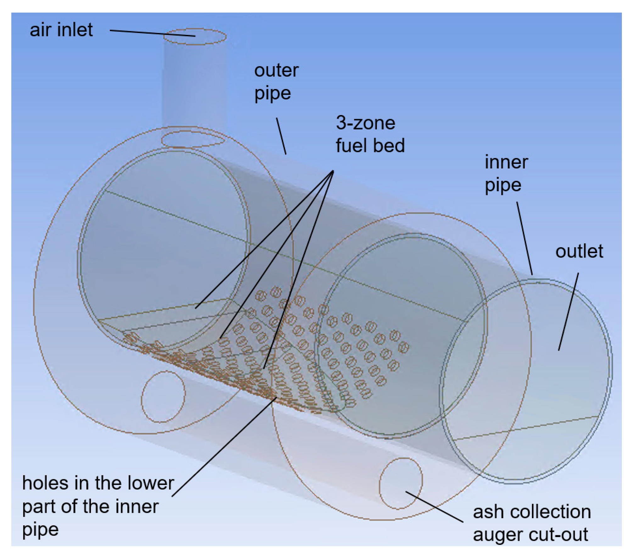
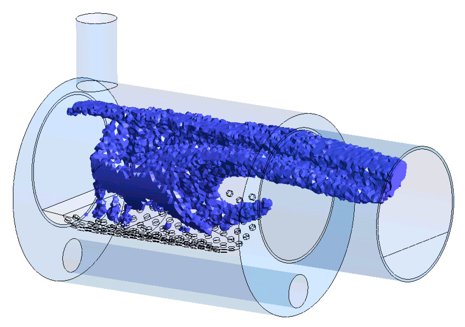
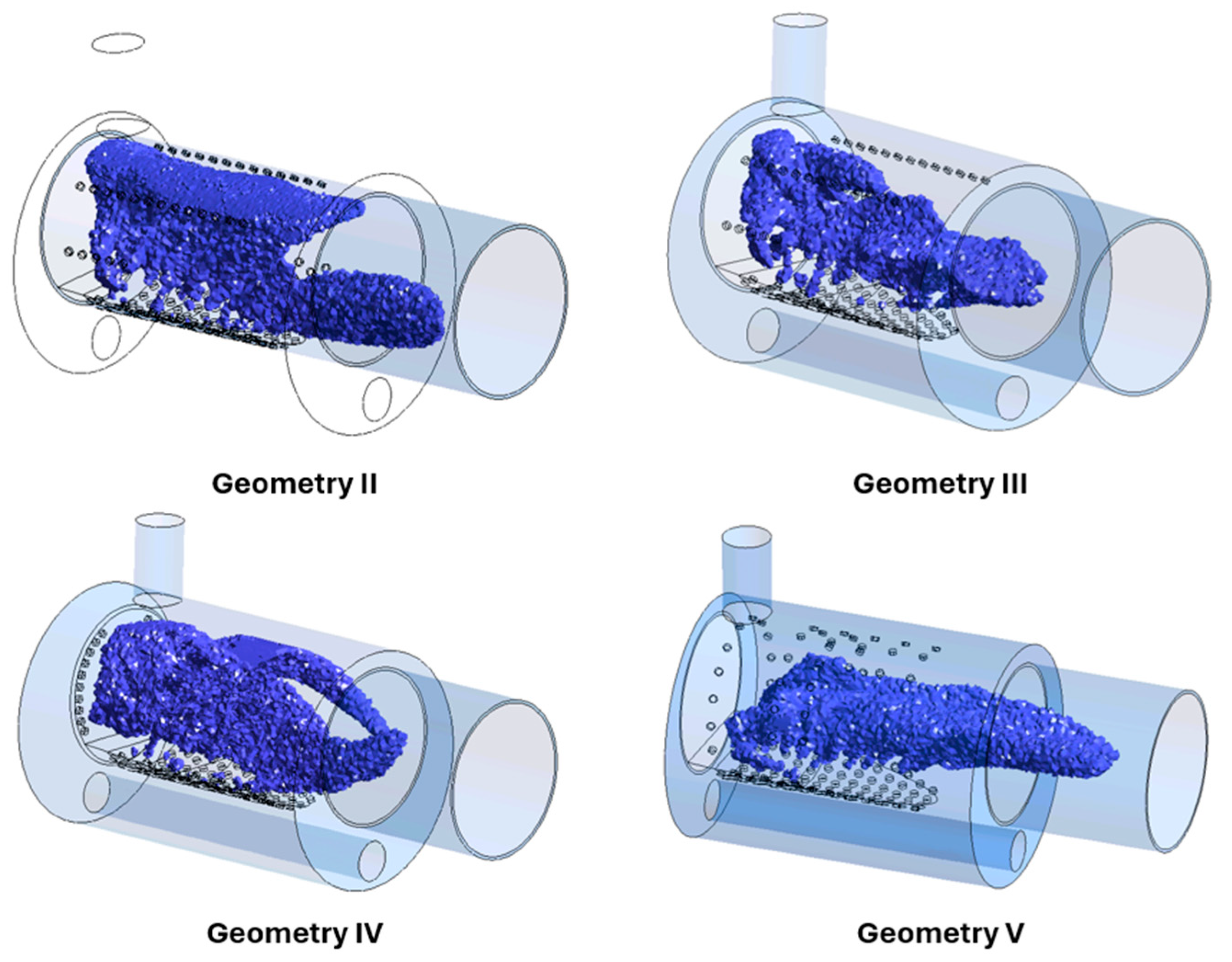
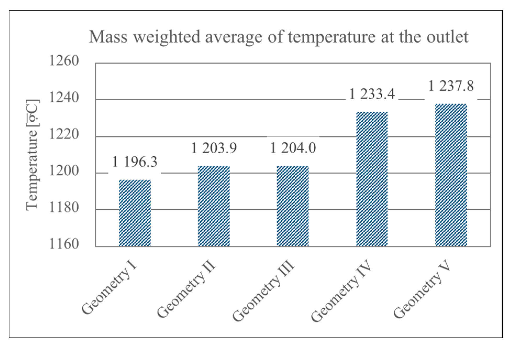
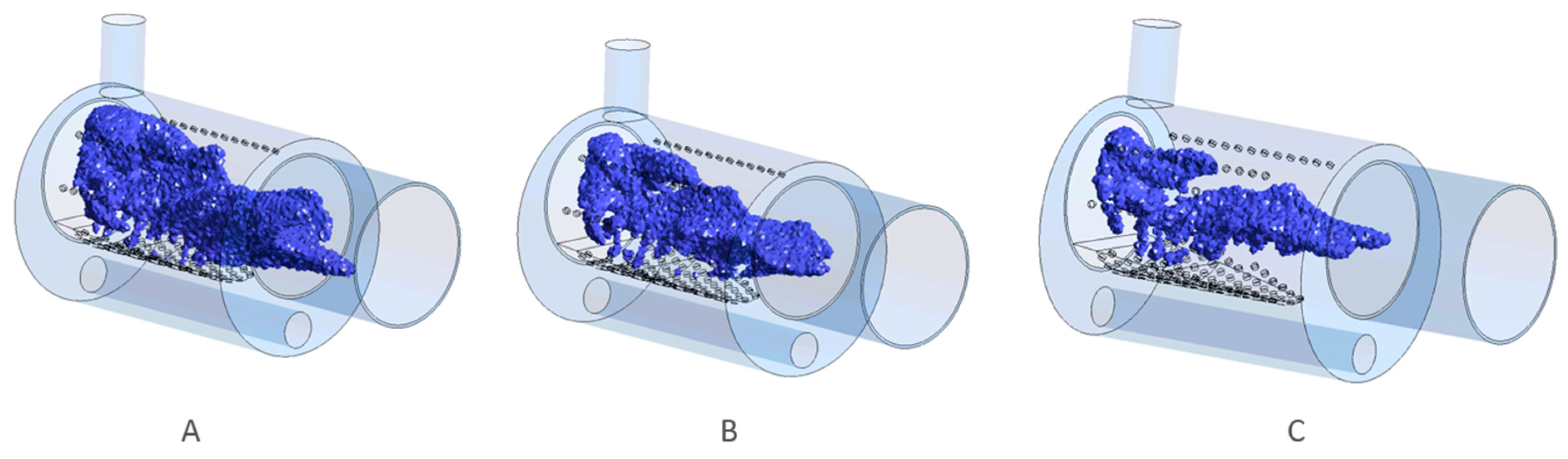
3.1. Geometry Optimization

The optimization of the burner’s geometry aimed to use secondary shielding air to protect the walls (especially the upper wall, made of steel) from the adverse effects of high-temperature gas streams. At the same time, attention was paid to the combustion reaction parameters, such as maintaining an appropriate oxygen concentration in the various zones and maintaining an appropriate outflow temperature. Four geometries were analyzed (Figure 3), and their main optimization parameters (the number of primary and secondary air holes) are summarized in

Table 2. Primary and secondary air hole distribution.

Geometry	I (Initial)	II	III	IV	V
Quantity of primary air holes	136	102	136	136	102
Quantity of secondary air holes	0	36	36	20	38

.

The first modification (geometry II) involved the addition of two levels of secondary air holes. Each hole had a diameter of 5 mm and was drilled radially. Additional rows of holes were positioned symmetrically on both sides of the burner, with the first row in the middle of the internal pipe covering combustion zones I and II. The upper row was nearly two times longer, aimed mainly at protecting the upper wall.

These changes caused the highest-temperature zone to shift downward, particularly in the second part of the burner. It was also observed that the air flowing through the grate holes (in the lower part of the burner) largely passed through the holes in the final part of the grate, those not covered by fuel, due to low flow resistance. This phenomenon results in restricted airflow under the grate in the first and second zones of the bed.

To limit the airflow through the uncovered holes in combustion zone III, a modification was introduced by sealing some of these holes (Figure 3, geometry III). This change positively affected the air distribution. Sealing part of the holes in the grate contributed to an increase in the gas flow through the secondary air holes, resulting in the highest-temperature zone being moved away from the upper wall of the burner and promoting a better mixing of the streams, thereby intensifying the chemical reactions.

Another geometry considered was a burner with secondary air supplied from the front (Figure 3, geometry IV). In this case, the design of the outer tube had to be modified as well. It was extended to allow the secondary air to flow in a plane perpendicular to the burner axis (Figure 3). The analysis of the results indicates that this is not an optimal burner configuration. The stream of hot exhaust gases “sticks” to the upper wall, especially in the regions of combustion zones II and III (Figure 4). There are also areas of oxygen deficiency, which affects the combustion reaction dynamics.

To move the zone of hot exhaust gases away from the upper wall and to minimize areas with excessively low oxygen concentration, a solution with a more uniform secondary air distribution was proposed (Figure 3, geometry V). In this geometry, the holes were arranged circumferentially, decreasing their number along the longitudinal coordinate of the burner. As seen in Figure 5, the zone with the highest temperatures shifted towards the burner axis. This was assessed to be the best of the considered burner geometries.

The geometries were also compared by outflow temperature. In all modified cases, the temperature was higher than in the initial case (Figure 6) and exceeded 1200 °C. The highest values were observed for geometries IV and V (1233.4 °C and 1237.8 °C, respectively), although a better distribution of the hot zone in the burner was noted in the case of geometry V (compare Figure 5).

Geometry V seems to fulfill the requirements in terms of the high-temperature zone’s position. This case is characterized by the highest outflow temperature (Figure 6). As can be observed in the modeling results (Figure 7A), temperatures above 1500 °C occur in the middle of the inner pipe. This confirms the initial conclusion that the thermal degradation of the burner walls was mitigated in this case. In further cross-sections (Figure 7B–E), combustible particle and combustion product concentrations are presented. The modeled combustible volatilities, like CH₄, C₆H₆, and CO, are mainly present in the neighborhood of zone II, and they are then transferred towards the burner outlet with the air/flue gas mixture. Their concentration decreases due to the chemical reactions. The main stream of increased particle concentration is directed below the burner axis, toward the outlet. The concentration of combustible particles decreases and becomes very low beyond the grate zone. The highest CO₂ concentrations can be observed near porous zone II, which is caused by fuel devolatilization and initial chemical reactions between the air and the other combustible species present in this zone. Further presence of CO₂ is derived from chemical reactions like char combustion to CO₂ (zone III) and mainly the combustion of other species (mainly CO, which is introduced as a fuel component but also as a semi-product of other species’ oxidation, as a two-step reaction model was used).

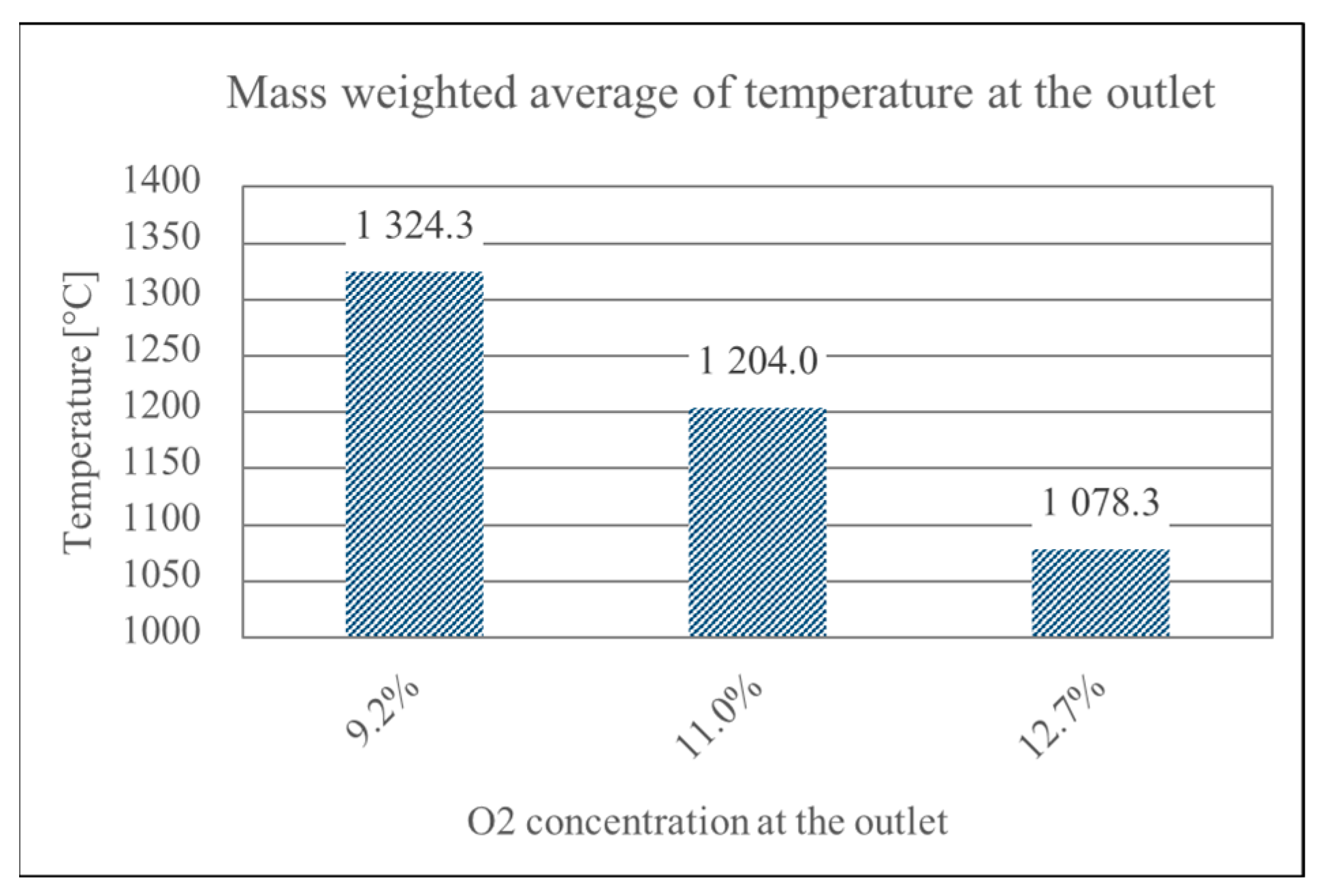
3.2. Air Mass Flow

As part of the conducted work, not only analyses concerning burner geometry but also analyses of the burner’s operating conditions were performed. Using the example of geometry III, a variant analysis of the burner operating conditions was conducted with varying air flow rates. This can be easily obtained by adjusting the airflow supplied for combustion. The airflow rate can be controlled by varying the rotational speed of the blower fan. Calculations were carried out for three air flow rates, corresponding to the following oxygen concentrations at the burner outlet: A—9.18%; B—11.01%; and C—12.69%. A higher oxygen concentration with a preserved amount of fuel and a preserved geometry of the burner was obtained by inserting a greater mass flow of air. This resulted in higher velocities in the domain, especially in the region after the inlet tube (Figure 8). A lower air flow rate caused a higher average exhaust gas temperature at the burner outlet (Figure 9). A greater amount of air also contributed to reducing the high-temperature zone and to its movement toward the burner’s axis (Figure 10 and Figure 11). In case C, the risk of the thermal degradation of the burner’s upper wall is limited, but the outlet temperature is also lower, although it still exceeds the required 1000 °C. With an increase in the supplied air flow rate, the water concentration in the outlet cross-section decreased (from 5.75% to just over 4% in case C), as did the CO₂ concentration—from 17.3% to 12.4%. A decrease in CO concentration with an increase in the air mass flow rate was also observed, along with a very slight increase in NOx emissions—from 142 mg/Nm³ to approximately 170 mg/Nm³.

The analysis of the inlet mass flow rate of air showed that even in an unoptimized geometry, when operational conditions change, the risk of thermal damage to the burner’s upper wall can be limited. It is to be highlighted that even in these conditions, burner operation allows the temperature of the required flue gases at the outlet to be greater than 1000 °C.

4. Discussion

Current energy policies force heat and electricity generation to move towards renewables. One of them can be solid biomass, which can be used in bio-CHP in the form of pellets. Although there are commercially available solid biomass burners, the fuel combustion process in such an installation requires the design of a new burner type to provide a high-temperature stream of flue gases at the outlet. An example of such a burner is shown in [20]. Unfortunately, its operation has revealed the risk of material degradation due to the influence of high temperature, especially in the upper wall zone. The authors have tried to overcome this problem by changing the secondary air distribution or changing the operating conditions of the example case.

First, geometry optimization was studied. Four geometries with secondary air holes were analyzed (geometries II–V). The best results were obtained in the case of geometry V—the high-temperature zone was moved toward the burner axis, so the risk of thermal damage to the walls was limited, and the outflow temperature (mass weighted average) exceeded 1230 °C (oxygen concentration 11%), so the required flue gas temperature in terms of its coupling with a Stirling engine was preserved. In this case, secondary air was inserted, mainly from the top wall of the burner, which helped to push the high-temperature zone far away from the wall, preventing the hot stream from touching the wall, which would make thermal degradation more likely. The changes in the air distribution did not have a negative influence on the combustion process (Figure 7). Nearly all combustible particles reacted in the grate zone or closely behind.

Another way to protect the burner walls against local high temperatures tested in this study is to increase the mass flow of air, which was studied using the example of geometry III. In this case, a nonoptimal geometry was selected to show the possibilities of achieving the desired effect even in such a case, which can be helpful, e.g., for existing installations. One should be aware that this method is linked to a decrease in outflow temperature, by approximately 125 °C in the analyzed case, which should be taken into account together with the requirements of the further installation. As can be concluded from the analysis carried out, this method can also be effective, although the goal was reached by limiting the high-temperature zone rather than by moving it to a different section of the burner.

5. Conclusions

• Geometry optimization mitigates thermal degradation: Modifying the burner geometry, especially the distribution of secondary air holes, significantly reduced the risk of thermal degradation of the burner’s upper wall. Geometry V proved most effective, successfully shifting the high-temperature zone away from sensitive wall areas and improving combustion stability.
• A high outlet temperature ensures Stirling engine compatibility: All optimized geometries achieved flue gas temperatures above the critical 1000 °C threshold. Geometry V achieved the highest outlet temperature (1237.8 °C), fulfilling the requirements of efficient heat transfer to the Stirling engine in micro-CHP applications.
• Increased air mass flow reduces wall overheating: Operational optimization by increasing the air mass flow rate (e.g., via blower adjustment) successfully limits high-temperature zones near burner walls—even in suboptimal geometries. However, this also leads to reduced flue gas temperatures, requiring a balance between structural protection and thermal performance.

References

- Gonzcalves, A.C.; Malico, I. Biomass for Domestic Heat BT—Forest Bioenergy: From Wood Production to Energy Use; Springer International Publishing: Evora, Portugal, 2024; pp. 209–233. ISBN 978-3-031-48224-3. [Google Scholar]
- World Bioegengy Association. Global Bioenergy Statistics 2022; World Bioegengy Association: Stockholm, Sweden, 2022. [Google Scholar]
- Niekurzak, M. The potential of using renewable energy sources in Poland taking into account the economic and ecological conditions. Energies 2021, 14, 7525. [Google Scholar] [CrossRef]
- Krawczyk, P.; Badyda, K.; Dzido, A. Techno-Economic Analysis of Increasing the Share of Renewable Energy Sources in Heat Generation Using the Example of a Medium-Sized City in Poland. Energies 2025, 18, 884. [Google Scholar] [CrossRef]
- Jonsson, R.; Rinaldi, F. The impact on global wood-product markets of increasing consumption of wood pellets within the European Union. Energy 2017, 133, 864–878. [Google Scholar] [CrossRef]
- Zhu, S.; Yu, G.; Liang, K.; Dai, W.; Luo, E. A review of Stirling-engine-based combined heat and power technology. Appl. Energy 2021, 294, 116965. [Google Scholar] [CrossRef]
- Chacón, J.; Sala, J.M.; Blanco, J.M. Investigation on the design and optimization of a low NOx-Co emission burner both experimentally and through computational fluid dynamics (CFD) simulations. Energy Fuels 2007, 21, 42–58. [Google Scholar] [CrossRef]
- Yan, W.; Li, K.; Yu, T.; Huang, X.; Yu, L.; Panahi, A.; Levendis, Y.A. Determination of Flame Temperatures and Soot Volume Fractions during Combustion of Biomass Pellets. Energy Fuels 2021, 35, 2313–2325. [Google Scholar] [CrossRef]
- Weng, W.; Feuk, H.; Li, S.; Richter, M.; Aldén, M.; Li, Z. Temporal temperature measurement on burning biomass pellets using phosphor thermometry and two-line atomic fluorescence. Proc. Combust. Inst. 2021, 38, 3929–3938. [Google Scholar] [CrossRef]
- Deore, S.P.; Gadkari, P.; Mahajani, S.M.; Kumar, S.; Kumar, S. Development of a new premixed burner for biomass gasifier generated low calorific value producer gas for industrial applications. Energy 2023, 279, 128140. [Google Scholar] [CrossRef]
- Costa, M.A.; Schiavon, N.C.B.; Felizardo, M.P.; Souza, A.J.D.; Dussán, K.J. Emission analysis of sugarcane bagasse combustion in a burner pilot. Sustain. Chem. Pharm. 2023, 32, 101028. [Google Scholar] [CrossRef]
- Zainith, P.; Mishra, N.K. Numerical study for the combustion analysis of wood volatiles in porous radiant burner for the application of biomass cooking stove. Int. J. Therm. Sci. 2024, 196, 108708. [Google Scholar] [CrossRef]
- Chen, C.Y.; Chen, W.H.; Hung, C.H. Combustion performance and emissions from torrefied and water washed biomass using a kg-scale burner. J. Hazard. Mater. 2021, 402, 123468. [Google Scholar] [CrossRef] [PubMed]
- He, F.; Wei, F.; Ma, C.; Zhao, H.; Fan, Y.; Wang, L.; Wang, J.A. Performance of an intelligent biomass fuel burner as an alternative to coal-fired heating for tobacco curing. Pol. J. Environ. Stud. 2020, 30, 131–140. [Google Scholar] [CrossRef]
- Marra, F.S.; Miccio, F.; Solimene, R.; Chirone, R.; Urciuolo, M.; Miccio, M. Coupling a Stirling engine with a fluidized bed combustor for biomass. Int. J. Energy Res. 2020, 44, 12572–12582. [Google Scholar] [CrossRef]
- Schneider, T.; Ruf, F.; Müller, D.; Karl, J. Performance of a fluidized bed-fired Stirling engine as micro-scale combined heat and power system on wood pellets. Appl. Therm. Eng. 2021, 189, 116712. [Google Scholar] [CrossRef]
- Borisov, I.; Khalatov, A.; Paschenko, D. The biomass fueled micro-scale CHP unit with stirling engine and two-stage vortex combustion chamber. Heat Mass Transf. Und Stoffuebertragung 2022, 58, 1091–1103. [Google Scholar] [CrossRef]
- Kropiwnicki, J. Low temperature rotary Stirling engine: Conceptual design and theoretical analysis. Appl. Therm. Eng. 2024, 257, 124276. [Google Scholar] [CrossRef]
- Sripakagorn, A.; Srikam, C. Design and performance of a moderate temperature difference Stirling engine. Renew. Energy 2011, 36, 1728–1733. [Google Scholar] [CrossRef]
- Krawczyk, P.; Kurkus-Gruszecka, M.; Wilczyński, M.; Dzido, A. Numerical analysis of design and operational parameters of low power pellet burners. Renew. Energy 2025, 243, 122577. [Google Scholar] [CrossRef]
- Ahn, J.; Kim, H.J. Combustion process of a Korean wood pellet at a low temperature. Renew. Energy 2020, 145, 391–398. [Google Scholar] [CrossRef]
- Biswas, A.K.; Rudolfsson, M.; Broström, M.; Umeki, K. Effect of pelletizing conditions on combustion behaviour of single wood pellet. Appl. Energy 2014, 119, 79–84. [Google Scholar] [CrossRef]
- Wiese, J.; Wissing, F.; Höhner, D.; Wirtz, S.; Scherer, V.; Ley, U.; Behr, H.M. DEM/CFD modeling of the fuel conversion in a pellet stove. Fuel Process. Technol. 2016, 152, 223–239. [Google Scholar] [CrossRef]
- Saldarriaga, J.F.; Aguado, R.; Pablos, A.; Amutio, M.; Olazar, M.; Bilbao, J. Fast characterization of biomass fuels by thermogravimetric analysis (TGA). Fuel 2015, 140, 744–751. [Google Scholar] [CrossRef]
- Cavalaglio, G.; Cotana, F.; Nicolini, A.; Coccia, V.; Petrozzi, A.; Formica, A.; Bertini, A. Characterization of various biomass feedstock suitable for small-scale energy plants as preliminary activity of biocheaper project. Sustainability 2020, 12, 6678. [Google Scholar] [CrossRef]
- Zadravec, T.; Rajh, B.; Kokalj, F.; Samec, N. CFD modelling of air staged combustion in a wood pellet boiler using the coupled modelling approach. Therm. Sci. Eng. Prog. 2020, 20, 100715. [Google Scholar] [CrossRef]
- Caretto, L.S. Modeling pollutant formation in combustion processes. Symp. Combust. 1973, 14, 803–817. [Google Scholar] [CrossRef]
- Launder, B.E.; Spalding, D.B. The numerical computation of turbulent flows. In Numerical Prediction of Flow, Heat Transfer, Turbulence and Combustion; Elsevier: Amsterdam, The Netherlands, 1983; pp. 96–116. [Google Scholar]
- Fletcher, D.F.; Haynes, B.S.; Christo, F.C.; Joseph, S.D. A CFD based combustion model of an entrained flow biomass gasifier. Appl. Math. Model. 2000, 24, 165–182. [Google Scholar] [CrossRef]
- Dixon, T.F.; Mann, A.P.; Plaza, F.; Gilfillan, W.N. Development of advanced technology for biomass combustion—CFD as an essential tool. Fuel 2005, 84, 1303–1311. [Google Scholar] [CrossRef]
- Murthy, J.Y.; Mathur, S.R. Finite volume method for radiative heat transfer using unstructured meshes. J. Thermophys. Heat Transf. 1998, 12, 313–321. [Google Scholar] [CrossRef]
- Hernik, B. Numerical Research of Flue Gas Denitrification Using the SNCR Method in an OP 650 Boiler. Energies 2022, 15, 3427. [Google Scholar] [CrossRef]
- Skreiberg, A.; Skreiberg, O.; Sandquist, J.; Sørum, L. TGA and macro-TGA characterisation of biomass fuels and fuel mixtures. Fuel 2011, 90, 2182–2197. [Google Scholar] [CrossRef]
- Hermansson, S.; Thunman, H. CFD modelling of bed shrinkage and channelling in fixed-bed combustion. Combust. Flame 2011, 158, 988–999. [Google Scholar] [CrossRef]
- Gómez, M.A.; Martín, R.; Chapela, S.; Porteiro, J. Steady CFD combustion modeling for biomass boilers: An application to the study of the exhaust gas recirculation performance. Energy Convers. Manag. 2019, 179, 91–103. [Google Scholar] [CrossRef]