1. Introduction
The peak shaving technique is one of the key mechanisms implemented in high-tech power grids, including rail networks, to reduce the need for costly peak-time power generation [
1,
2]. In the past, the problem of peak load was often solved by increasing power [
3]. A certain percentage of the total installed power was reserved for peak load management, while the rest of the power was allocated to the base load. However, this solution leads to the inefficient use of electricity generators. They were only used to their full capacity at certain times. This solution also has several other disadvantages, such as higher energy consumption, greater wear and tear on equipment, and higher maintenance costs [
3,
4]. Potential strategies for peak shaving are demand-side management, integrating energy storage systems, and integrating photovoltaic and energy storage systems [
5]. Energy storage for peak shaving can be used in industry, residential buildings, and microgrids. In general, peak shaving is realized by charging the energy storage when the energy demand is low (off-peak period) and discharging it when the demand is high (peak period) [
6].
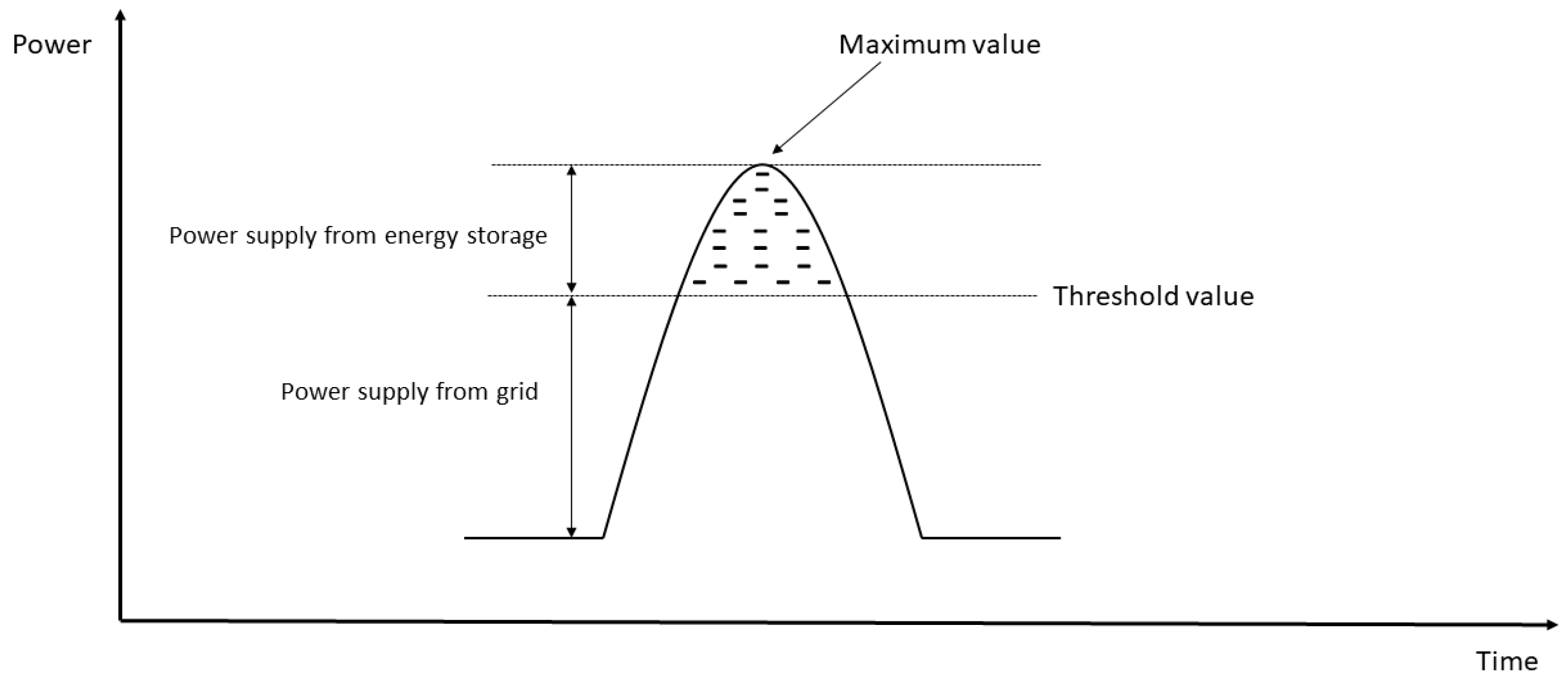
Figure 1 shows a schematic representation of the peak load reduction concept using an energy storage system.
As shown in
Figure 1, the energy storage system is activated when the threshold load power is exceeded. Utilizing the energy storage system brings specific economic benefits as it reduces the demand for expensive peak electricity production. The real advantage of peak load reduction based on energy storage is that it reduces peak demand while maintaining the comfort of an adequate level of electricity. The use of energy storage systems is also necessary due to the discontinuous nature of electricity production by renewable energy sources [
7,
8]. Microgrids, especially islanded microgrids, are characterized by a high variability of energy demand over time, manifesting in the form of peaks in the load profile. If the power generation system is not perfectly matched to the time characteristics of the electricity demand, several problems arise. The most serious of these include instability in electricity supply, voltage fluctuations, and a general reduction in reliability, all of which ultimately result in a poor-quality power supply [
9,
10]. It should be remembered that power systems are often designed to be oversized to meet peak load requirements. As a result, when the system is operating at partial load, some system components, such as transformers, are less efficient [
11,
12]. Since microgrids are small, they usually do not contain a peak generator like the main distribution power systems. In some solutions, a certain percentage of the total power (at least 10%) creates an energy reserve to cover peak demand. For example, small diesel and gas generators mainly supply this reserve power. However, this type of power plant has high operating and maintenance costs [
13]. In general, the advantages of using peak shaving can be divided into technical, economic, and environmental ones. The undoubted technical advantages include the improvement of the power supply quality, an increase in the efficiency of electricity use, and a reduction in energy losses. Other important factors include integration with renewable energy sources, an increase in the reliability of the microgrid power supply, reactive power compensation, and an increase in the efficiency of the transmission and distribution infrastructure [
14,
15]. The economic advantages include lower costs related to transmission fees, no need for expensive peak generators, lower costs related to power reserves, lower operating costs, and the longer service life of the power system [
16,
17]. Peak shaving has various environmental benefits, the most important of which is the possibility of replacing inefficient and polluting generators. Furthermore, using a solution based on renewable energy sources with energy storage systems significantly reduces carbon dioxide emissions in electricity production [
18,
19]. The most promising solution for reducing peak loads is the connection of energy storage systems to the power grid [
20]. Energy storage systems based on electrochemical batteries are up-and-coming due to their high efficiency, short response time, and ease of scalability. Currently, the most common battery energy storage systems are lithium-ion, NaS, or REDOX flow batteries [
21]. Despite the potential benefits of energy storage systems for peak shaving, their implementation has several obstacles. The main problem is determining the optimal size of the energy storage facility. Installing an energy storage facility with a suboptimal size (capacity) can result in higher system losses and an inappropriate increased capital investment in the energy storage system. It is challenging to design an energy storage system for optimal performance. The advantages of this solution undoubtedly include a reduction in peak demand without compromising the quality of the electricity supply to the end user. Support for reactive power compensation is important and leads to a significant reduction in the operating costs of the power system [
22,
23]. It should also be recognized that reducing actual peak demand is difficult because actual peak demand can often be unexpectedly higher or occur with a duration that is much more extended than forecast based on the analysis of historical data [
24]. Electric railway networks present unique challenges and opportunities for peak shaving. Railway traction power demand is characterized by short sharp peaks caused by train accelerations and an overall intermittent load profile. Managing these peaks is important because railway operators often face significant demand charges from power companies, and the infrastructure must be dimensioned to handle the highest occurring peak power. In this way, peak power reduction can translate into significant cost savings and potentially postpone costly upgrades to power equipment. Flattening demand also reduces the load on the transmission grid during peak train traffic hours, which can improve the overall stability of the grid and reduce the likelihood of voltage drops or train-induced overloads [
25]. Peak shaving can also involve reducing the size of electrical infrastructure in railway systems. If effective peak demand is reduced, future substations and power supply networks can be designed with lower ratings, saving capital costs [
26]. Furthermore, if peak shaving is achieved through an on-site energy storage system (railway microgrid), it can provide a degree of backup power and resilience. Furthermore, the same energy storage system used for peak shaving can help run base loads during off-peak hours or maintain system voltage during disturbances. In railway networks, peak saving is realized through several approaches. A simple method is to implement stationary energy storage systems at traction substations. By installing energy storage systems and connecting them to the railway traction line, the energy storage systems can charge during periods of low demand and discharge to supply energy when the train’s power demand increases. This effectively limits the so-called net consumption from the distribution network. It is important to select the size of the storage facility optimally and to control the storage facility in the microgrid to maximize the benefits of energy saving [
27].
This article presents two methods of reducing the peak load of the railway traction substation. The first method is based on a variable threshold value at which the load reduction occurs. The second method involves the use of the immediate inter-peak battery charging of the energy storage system and the use of a fixed threshold value for load reduction. The strategy for choosing the method depends on the characteristics of load and traction network changes and their prediction for the time window relevant to the battery energy storage system charging time. A method for predicting time-dependent load based on the Poisson distribution and Long Short-Term Memory is presented. Based on the results, a peak shaving method was selected using the operation of one of the Polish traction substations as an example. Tests were carried out in the actual operating conditions of the railway microgrid in the analyzed traction substation.
2. Peak Shaving in an Energy Railway Microgrid
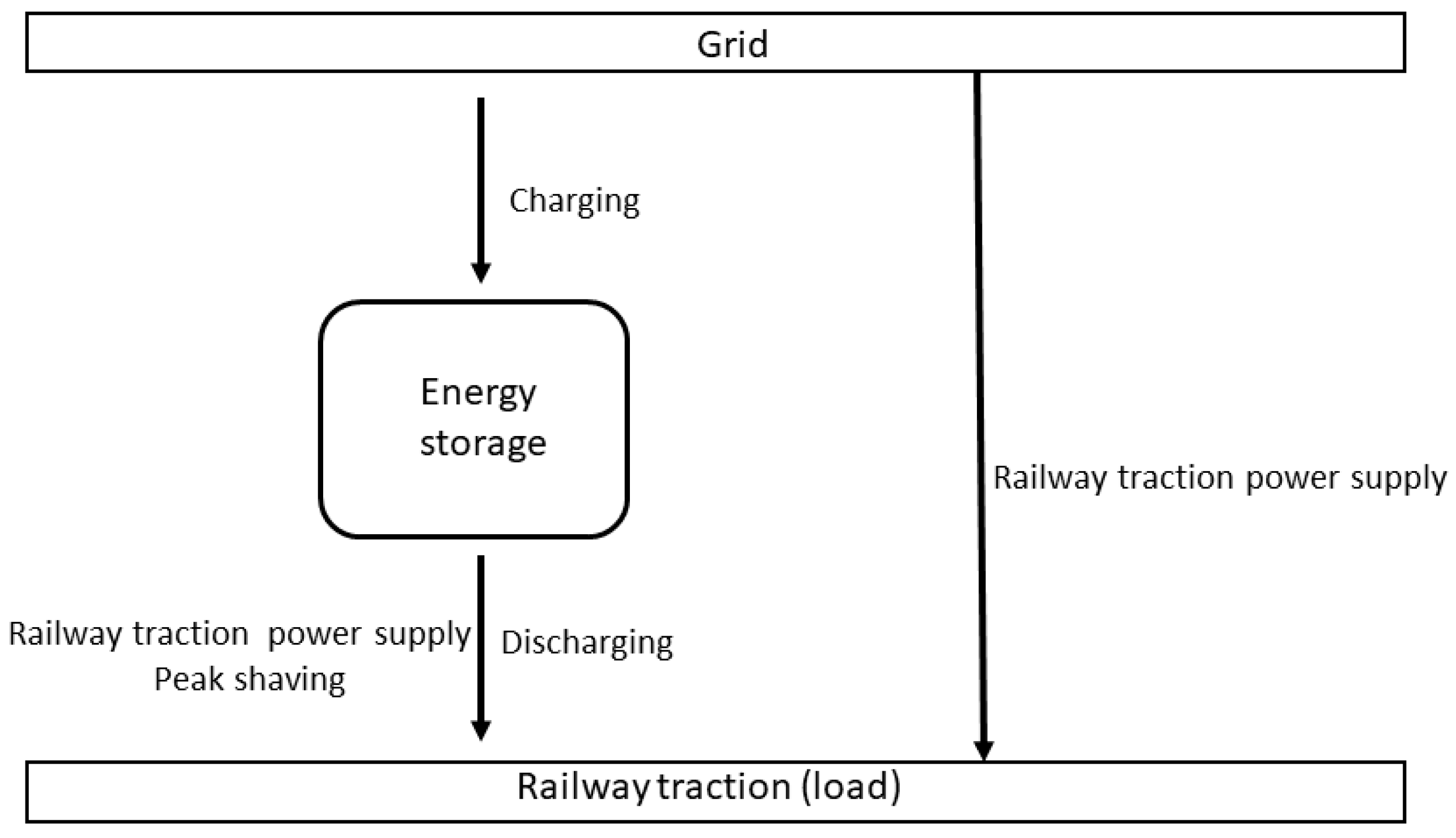
Figure 2 shows the power system consisting of a grid, a battery energy storage system, and a railway traction line in a simple railway microgrid for peak load reduction.
In the system shown in
Figure 2, the railway traction line is supplied with power from the grid. The energy stored in the battery energy storage system is used for the peak shaving procedure on the traction load. The grid charges the battery energy storage system. The energy storage system supplies energy to the loaded railway traction line during a specific peak load duration to reduce the power drawn from the grid. The threshold value of the power, and, thus, the size of the peak shaving, at which the stored energy is used depends on the battery energy storage system’s capacity. If the stored energy is reduced, then the possible size of the load reduction is smaller.
The area under the load curve (
Figure 3) represents the required energy from the battery energy storage system (E
mag) necessary to reduce the load power (P
l) when the power demand exceeds the threshold value (P
th). The corresponding power to be supplied from the energy storage system at a specific time (t
1, t
2), P
bes(t), is equal to the difference between P
l(t) and P
th(t) as follows [
28].
The area under the curve, which is the energy value from the battery energy storage system, is equal to the following.
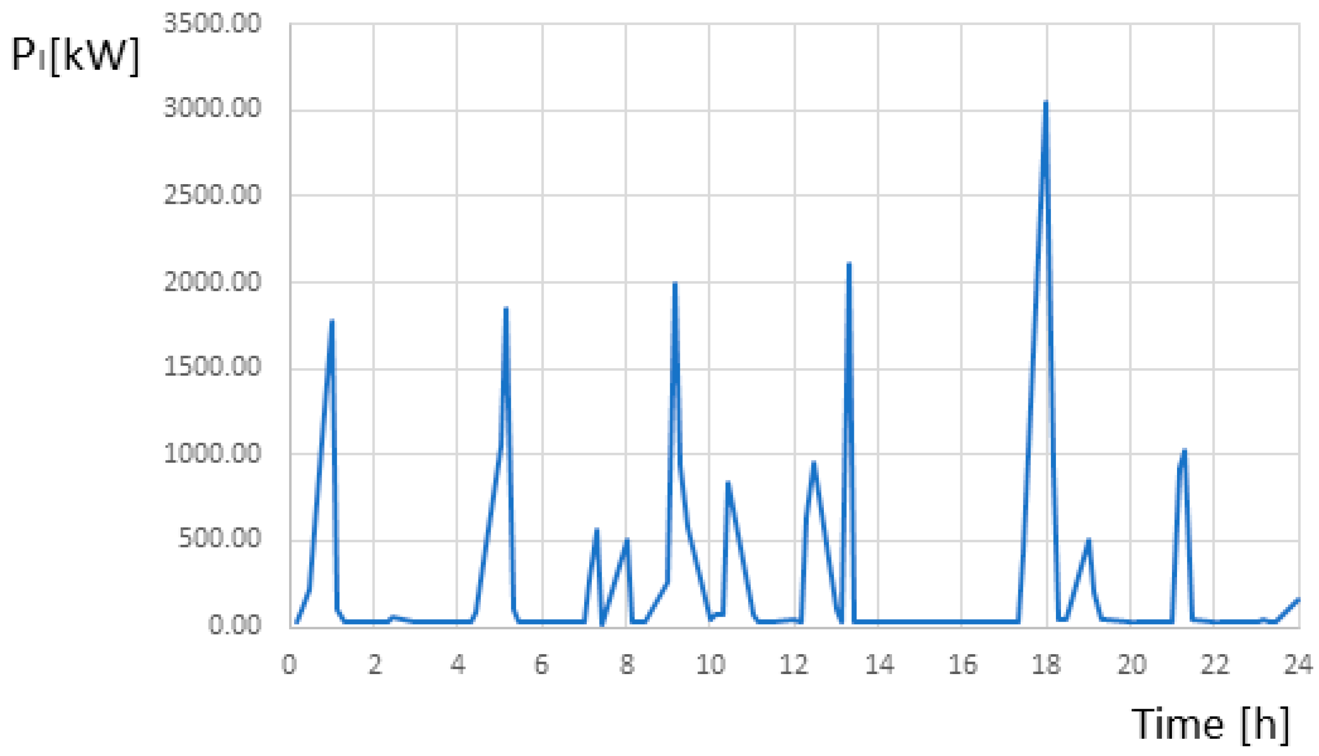
When the railway traction line is loaded, there is usually no broad daily peak load. The characteristic feature is repeated short load peaks (spikes) with different maximum values.
Figure 4 shows an example of the daily load profile of the railway traction line.
The individual peak of traction load can be approximated by a Gaussian curve in the following form:
where P
l,max is the maximum peak value, wg is the coefficient that scales the width of the peak curve, and t is time.
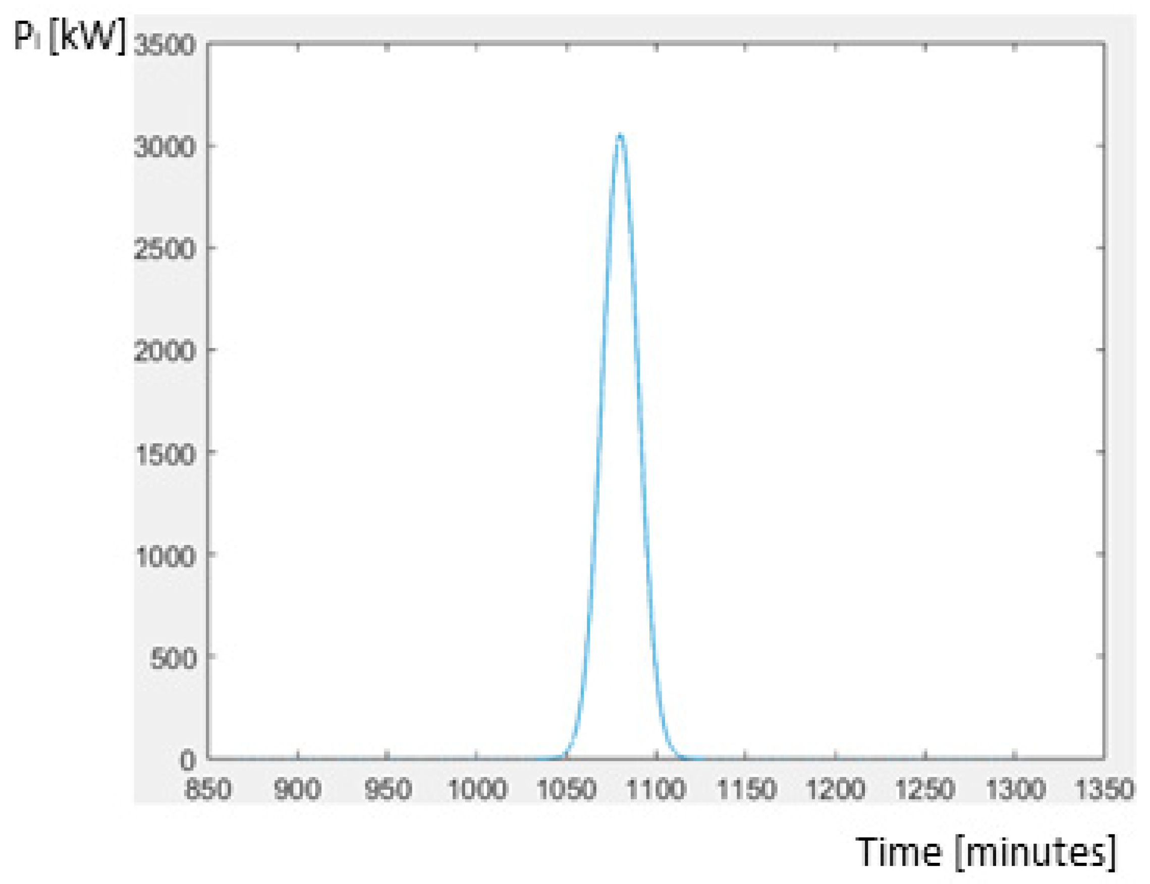
In the case of the greatest railway traction loads (peak at 6 p.m. in
Figure 4), which are the main target of peak load reduction, the course of the power change over time is well described by a Gaussian curve, described by the relationship (3), with a coefficient of wg = 0.947.
Figure 5 shows the course of the Gaussian curve with the value P
obc,max = 3054 kW and wg = 0.947.
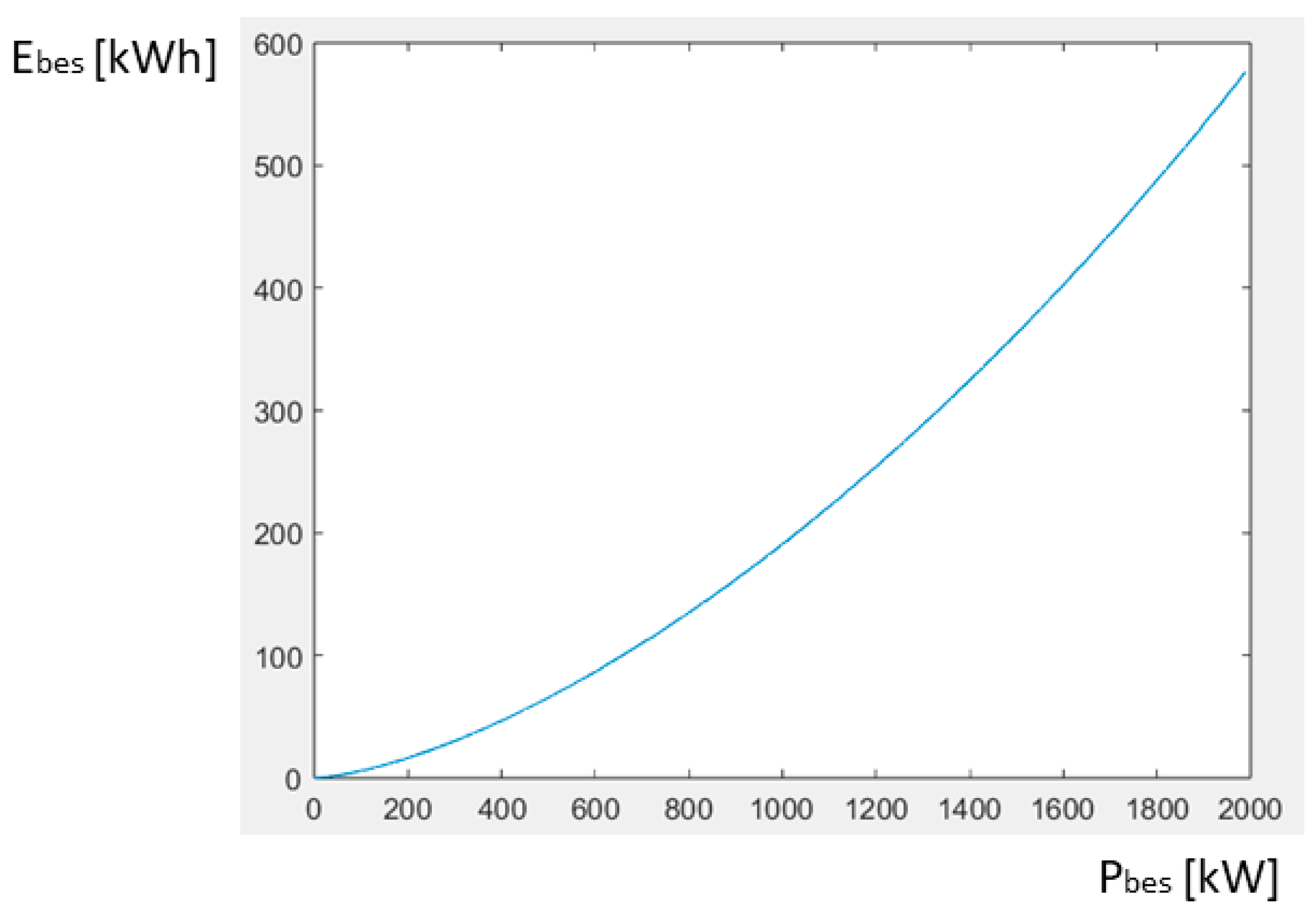
Figure 6 shows the relationship between the power P
bes = P
l,max − P
th and the energy from the battery energy storage system E
bes.
The relationship shown in
Figure 6 can be described by the following relationship:
with an R-squared coefficient of 0.9999.
When reducing the peak load of the railway traction, how the battery energy storage system is charged is of key importance. A problem arises when there is a need to repeat the procedure of peak shaving, and the battery energy storage system charging is planned for a time other than between two consecutive peak loads. This is typical for the so-called time-based method of charging energy storage systems. In the case of
Figure 4, this occurs when the storage facility’s charging occurs, for example, between 2:00 a.m. and 4:00 a.m. Suppose we assume that there are two maximum loads on the railway traction in quick succession and that there is no charging of the energy storage system between them. In that case, we can have two scenarios related to reducing the load capacity for the second peak.
Figure 7 shows case a, i.e., the peak load reduction for the first peak. For the second peak, two situations are presented: maintaining the Pth threshold value as for the first peak (case b) and increasing the P
th threshold value (case c).
Table 1 shows the power values P
th and P
bes and energy E
bes for a system with two load peaks and without energy storage during the time between the load peaks. Index 1 refers to the first peak load subjected to peak shaving. Index 2a refers to the second peak load subjected to peak shaving while maintaining the same threshold value as for the first peak load. Index 2c refers to the second peak load subjected to peak shaving while changing the threshold value.
It is assumed that the energy storage capacity is 1.2 MWh and the peak load is 3.054 MW. The energy from the battery energy storage system used to reduce the first peak was 600 kWh and 360 kWh for the second peak.
The problem of fully reducing successive peak loads on the railway traction can, thus, be solved by using a solution based on changing the threshold value depending on the level of charge in the battery energy storage system or by using the fast interpeak charging of the battery energy storage system after the first reduced peak load with a constant threshold value.
3. Method Based on the Variable Threshold Value
The method of matching the threshold value to the state of charge of the battery energy storage system can be applied when there is no storage charging between peak loads on the railway traction line. This method’s assumption is to reduce the peak load as shown in
Figure 7c fully. The threshold values P
th were determined in relation to the value P
l,max for different values of the depth of discharge (DOD) indicating the percentage by which the battery energy storage system is discharged The calculations were performed for battery energy storage systems with a capacity of 400 kWh, 800 kWh, 1.2 MWh, 1.6 MWh, and 2.0 MWh (
Table 2,
Table 3,
Table 4,
Table 5 and
Table 6).
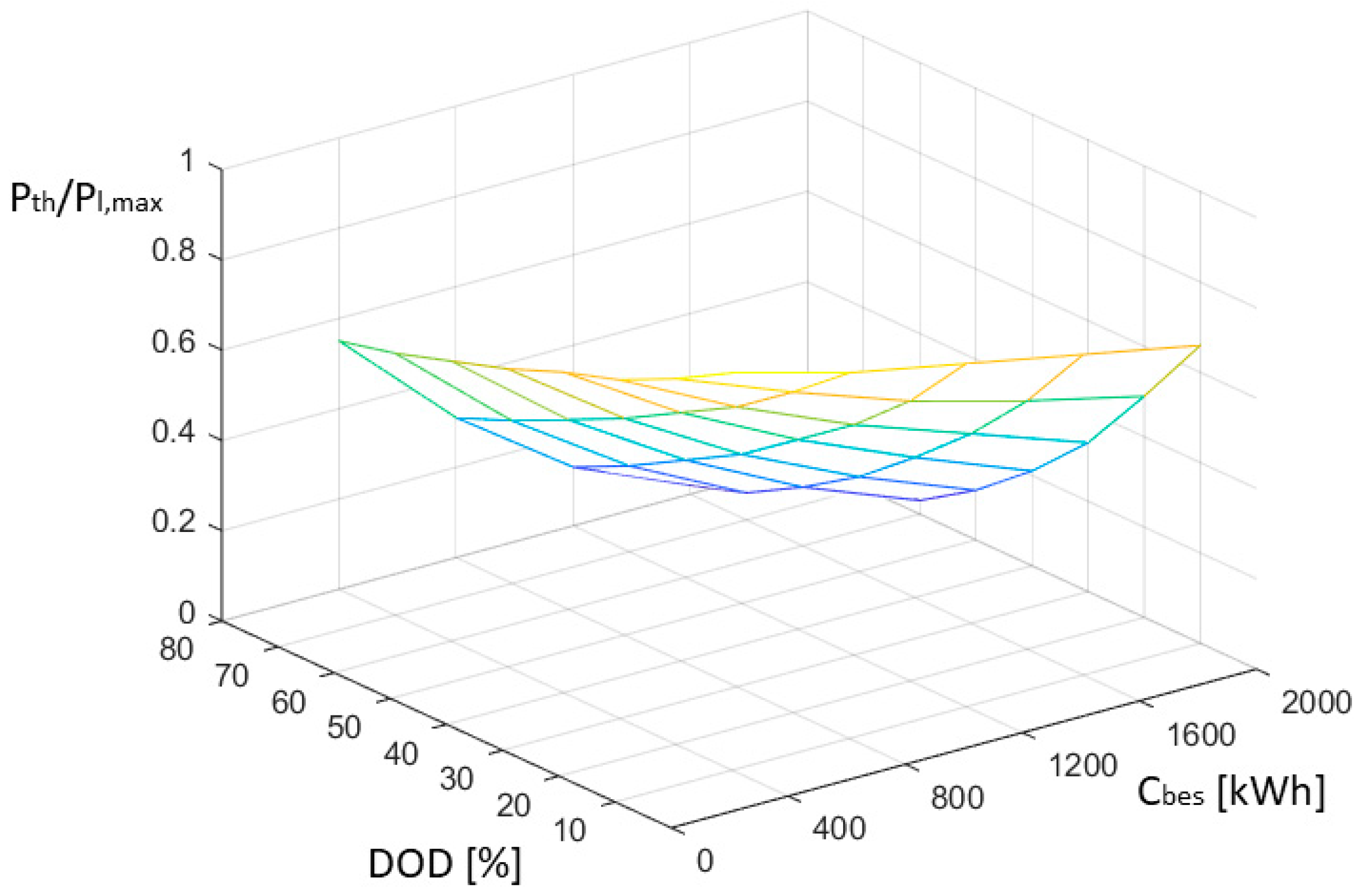
Figure 8 shows the relationship between the depth of discharge (DOD) value, battery energy storage system capacity (C
bes), and P
th/P
l,max.
Based on the graph in
Figure 8, the relationship between the threshold value P
th (given in kWh), the depth of discharge DOD (given in percent), and the battery energy storage system capacity C
bes (given in kWh) can be represented by the following equation:
with an R-squared coefficient of 0.9351.
Using relation (5), it is possible to determine the threshold value, depending on the state of discharge of the battery energy storage system, at which the peak shaving takes place for its entire duration. In addition, we can determine the number of consecutive peak loads on the railway traction based on historical load data. We can reduce the assumed number of peak load peaks on the network by selecting a threshold value.
For example, assuming a maximum depth of discharge for the battery energy storage system of 80%, then, for storage of 1.2 MWh, and assuming a depth of discharge for each peak of 20%, we can reduce the peak load for four peaks at Pth = 0.62∙Pl,max. In contrast, if we assume a depth of discharge of 40%, we can only reduce the peak load for two consecutive peaks at Pth = 0.42∙Pl,max.
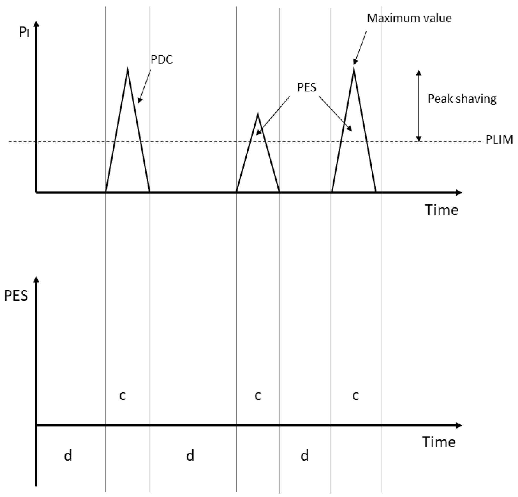
4. Method Based on the Inter-Peak Charging of a Battery Energy Storage System and the Fixed Threshold Value
The following is a peak shaving method based on the inter-peak charging of a battery energy storage system and a fixed threshold value. This method combines the fast-charging method and the low-power threshold method. Such a method is handy for power loads typical of a railway traction link, where a series of isolated load peaks characterize the load waveforms.
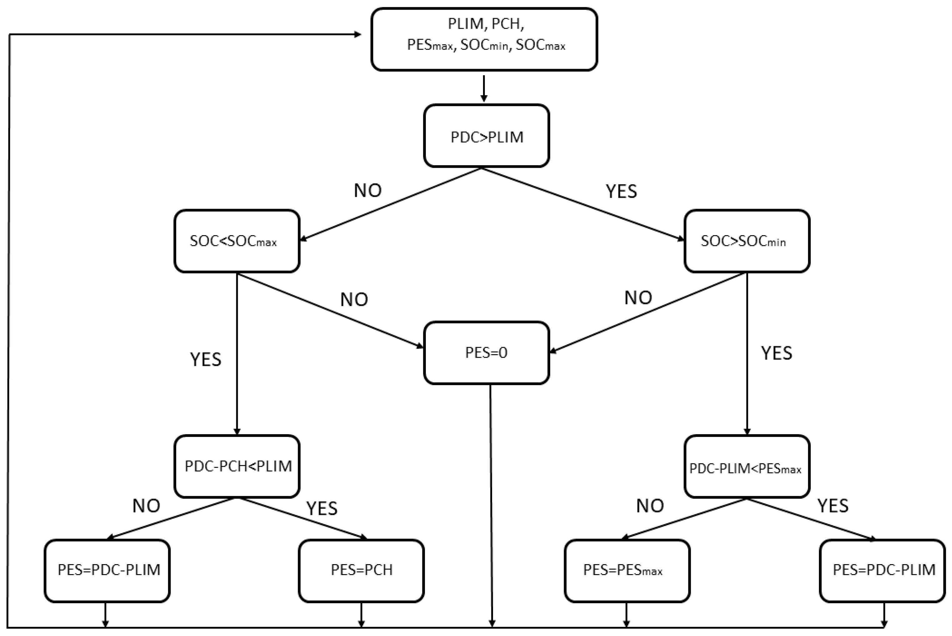
Figure 9 shows the energy storage control algorithm. The algorithm relates to the power architecture shown in
Figure 1.
The input data are the value of the power reduction threshold PLIM, the value of the charging power limitation of the battery energy storage system PCH, the maximum power coming from the battery energy storage system PES
max, and the value of the state of the charge of the battery energy storage system SOC (including the permissible values of the minimum and maximum charge level of the storage, i.e., SOC
min and SOC
max). The main parameter measured is the load power of the railway traction line PDC. The PDC power is compared with the PLIM power reduction threshold setting. This comparison constitutes the overriding control loop. The comparison result determines the operation mode of the battery energy storage system. Suppose the PDC power of the railway traction load is greater than the PLIM value, and the state of charge of the battery energy storage system is greater than the SOCmin value. The battery energy storage system is discharged with PES power in that case. This PES power is equal to the difference between the instantaneous value of PDC power and PLIM power, but it cannot be greater than the value of PES
max. If the charge level of the battery energy storage system is less than the SOC
min value, there will be no power flow from the battery energy storage system. If the load power of the PDC railway traction line is below the PLIM value and the state of the charge level of the battery energy storage system is below the SOC
max value, the process of charging the battery energy storage system with PES power takes place to prepare the system for the next process of the peak shaving of the railway traction load. No PES power consumption will occur if the battery energy storage system reaches the maximum charge level SOCmax. If the sum of the PCH limitation of the charging power and the power of the current PDC railway traction line load is below the established PLIM threshold, the charging of the battery energy storage system will occur with the PES power limited to the PCH power. If the sum of the PCH charging power and the power of the current load on the PDC railway traction is above the established PLIM threshold, the PES power with which the battery energy storage system is charged is reduced so that the sum of PES and PDC is below the value of the PLIM power reduction threshold. The algorithm ensures that, when there is no train traffic on the peak-load railway line, the battery energy storage system is charged with low power, for example, from the national distribution network. When a train appears on the section fed by a particular substation and the traction power demand of the PDC is detected, the battery energy storage system gives up energy quickly and provides the appropriate power level (
Figure 10). As a result, much less power is drawn from the grid while the train is in motion, significantly reducing the ordered peak power.
The variable threshold method involves the repeated application of peak shaving with a single charge of the battery energy storage system, which takes place outside peak hours of the traction line load. The reduction in subsequent peak loads is strongly dependent on the initial charge level of the battery energy storage system and the strategy adopted for reducing successive peak loads subjected to peak shaving. Subsequent reductions in peak loads occur when the thresholds for triggering the peak shaving procedure are raised. Its use is justified when the time intervals between the occurrence of reduced loads are shorter than the battery energy storage charging time. In the event of temporally separated peaks in the traction line load, it is possible to effectively charge the battery energy storage system between the peaks subject to peak shaving. This is conditional on the intervals between these peaks being longer than the battery energy storage charging time. In this case, there is a constant predetermined reduction in load peaks.
5. Selection of the Peak Shaving Method Based on the Prediction of Traction Load
The choice between the method with a variable threshold value and the method based on the inter-peak charging of a battery energy storage system and a fixed threshold value depends on whether, after a peak load that is subject to the peak shaving procedure, there are further loads requiring reduction during a time equal to the time of battery energy storage system charging (
Figure 11).
If the next load on the overhead line that exceeds the threshold value is within dT
bes (
Figure 11), the method with a variable threshold value should be used. Otherwise, the method is based on the inter-peak charging of the battery energy storage system and fixed threshold values used. The Poisson distribution method and the Long Short-Term Memory method were used to predict the number of peak loads exceeding the threshold value within the battery energy storage system charging time interval (dT
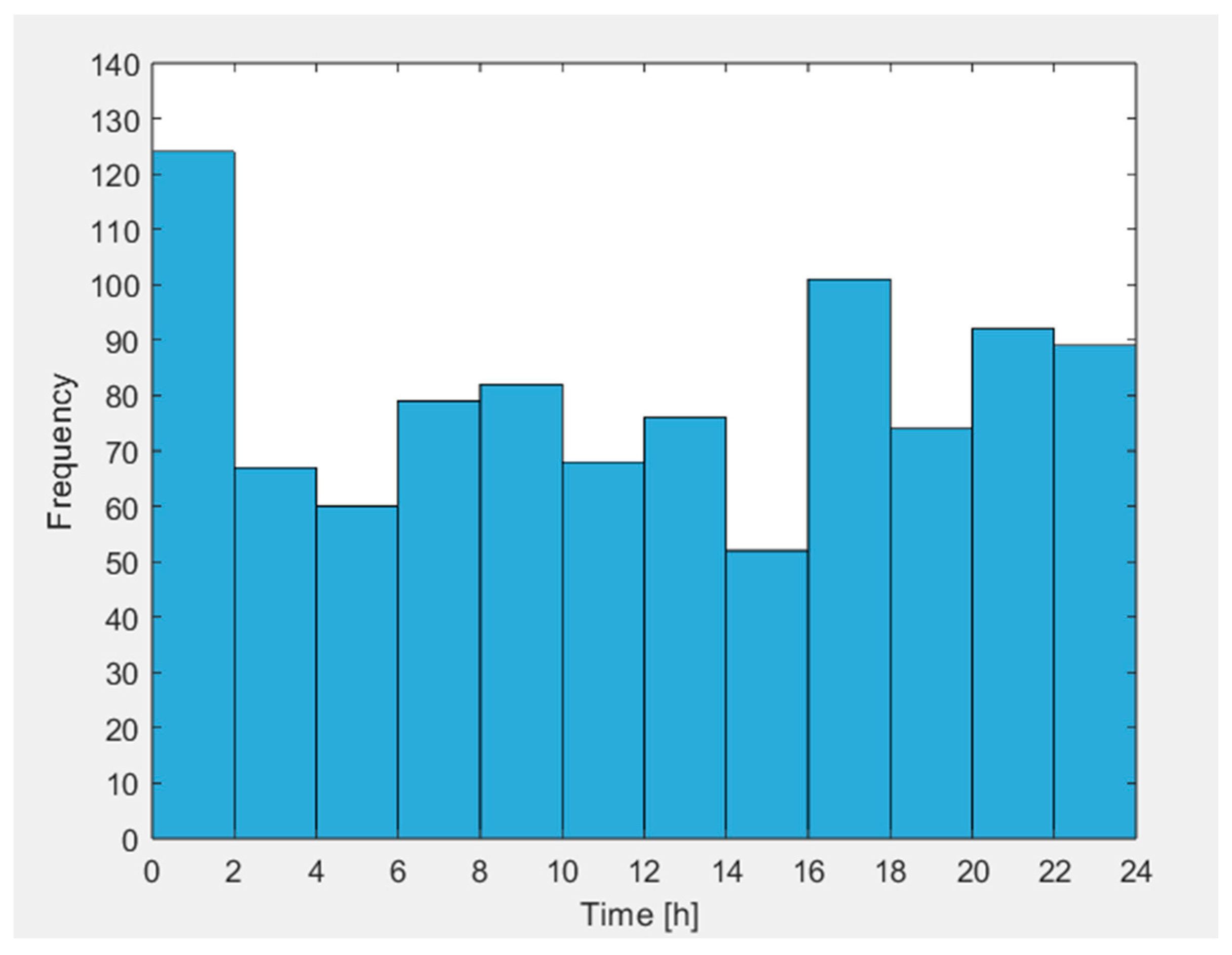
bes). The calculations included the traction substation electricity load data from the central repository for measurement data of the PGE Energetyka Kolejowa (Polish Railway Power Company). Data on the traction line load at the Grabce Zmigrod traction substation (51°30′47″ N 16°53′03″ E) were used for the period from 1 January 2022 to 31 December 2023. The traction load measurements covered 24 h periods with a measurement interval of 15 min. A threshold value of 1.0 MW was adopted.
Figure 12 shows a histogram of the daily number of occurrences of railway traction line loads exceeding the threshold value for 2023.
- (1)
Method using Poisson distribution
The Poisson distribution is often used to model the number of events in a given time interval when these events occur randomly but with a certain average frequency. In the context of predicting time events based on historical events, the Poisson distribution can be used under the following assumptions:
- (a)
events are independent of each other, i.e., the occurrence of one event does not affect the other;
- (b)
the probability of an event occurring in a given time interval is proportional to the length of that interval;
- (c)
the average number of events in a given time is constant (stationarity of the process).
The Poisson hypothesis served as a model to analyze the train flow in discrete statistically short time intervals. The analyzed time intervals were 2, 4, and 6 h. Independence refers to the number of trains at these intervals. The validity of this assumption, which is necessary for applying the Poisson distribution, was verified by the autocorrelation test, obtaining statistically acceptable results for >90% of the analyzed time windows. For the analyzed case of the railway traction line load, it can be assumed that Poisson assumptions are met.
In the Poisson-distribution-based prediction method, the key element is the estimation of the parameter λ, which represents the average number of events per unit of time. The value of this parameter is equal to the quotient of the number of events in the past and the total observation time. After determining the value of λ, the probability that a specific number of events will occur in a future time interval can be calculated according to the following relationship:
where k is the number of events in a specific time period.
Table 7 shows the probability of the number of occurrences of a railway traction contact line load exceeding the threshold value (P
ne) for a time dT
bes equal to 1 h, 2 h, 3 h, 4 h, 5 h, and 6 h.
Table 7 distinguishes between the probability of no such event occurring (P
ne = 0), the occurrence of one such event (P
ne = 1), and the occurrence of more than one such event (P
ne > 1). The value of P
e determines the most probable number of such events.
In the case of an analysis based on the Poisson distribution for dTbes equal to 1 h, 2 h, 3 h, and 4 h, the most likely event is that no railway traction load exceeding the threshold value will occur. However, for dTbes equal to 4 h, the difference between Pne = 0 and Pne = 1 is slight at only 1%. For dTbes of 5 h, it is most likely that one railway traction load exceeding the threshold value will occur. For 6 h, on the other hand, it is most likely that two such events will occur.
- (2)
Long Short-Term Memory method
The Long Short-Term Memory method is a type of Recursive Neural Network designed to process and predict sequences of events. Unlike classic Recursive Neural Network methods, the Long Short-Term Memory method solves the so-called vanishing gradient problem, thus enabling long-term dependency modeling. The LSTM method is very often used in time series analysis. The method copes well with sequential data, retaining information about long-term dependencies and memorizing previous events and their impact on the future [
29,
30]. It has also been used in analyzing the operating characteristics of the rail network, including the prediction of railway traction line loads [
31,
32]. The method was developed by S. Hochreiter and J. Schmidhuber in 1997 [
33]. In [
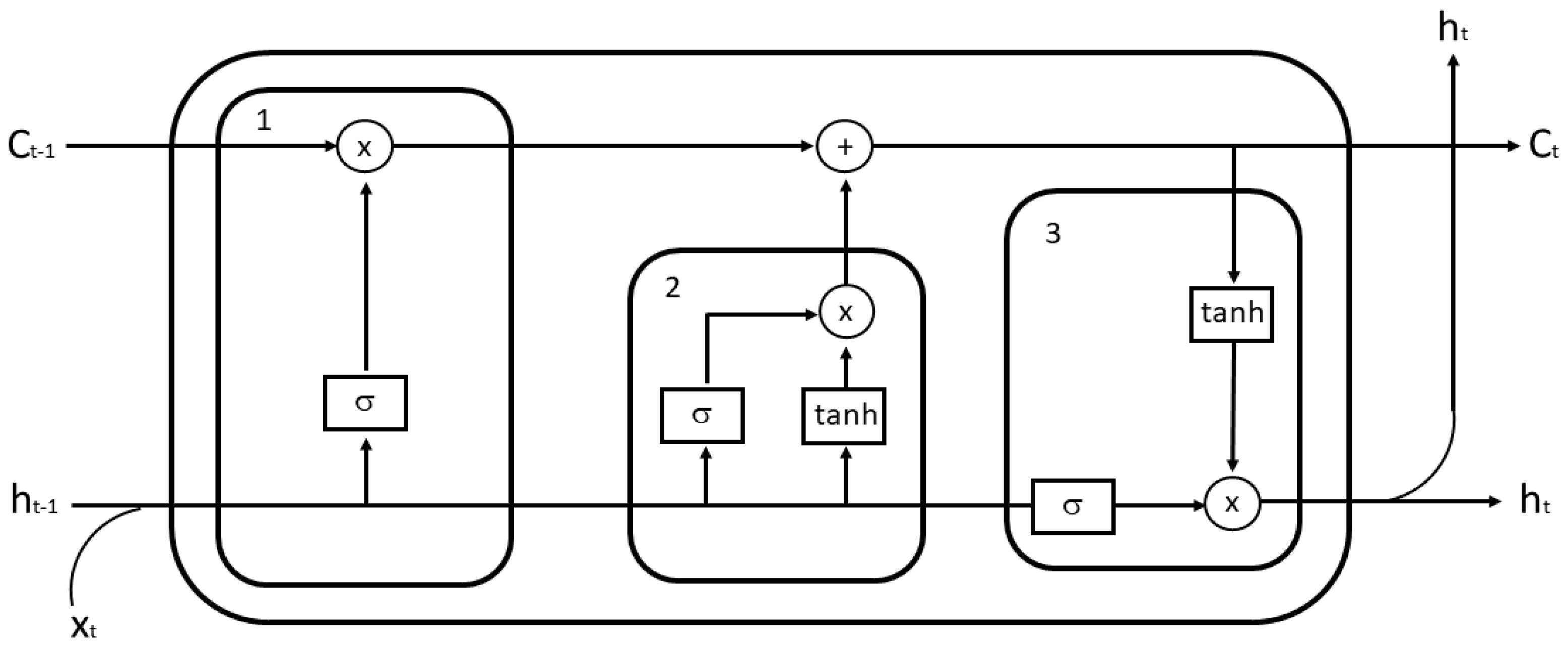
34], F. Gers, J. Schmidhuber, and F. Cummins introduced a forget gate into the architecture of this network. The fundamental element of Long Short-Term Memory is a memory cell. Each cell has three gates that control the flow of information. The input gate (i
t) is responsible for selecting values from the input to the modified memory, i.e., it controls which new values are added to the memory state. The sigmoid activation function σ determines which input values are relevant and are passed on to the memory. The tanh function then assigns a weight to the input values, determining their relevance. The values are processed by tanh to obtain a target value between −1 and 1. The output gate (o
t) determines which part of the internal memory status is transferred to the input of the next cell. The forget gate (f
t) decides which values from the previous state should be deleted. The sigmoid function σ is used to implement this functionality. The output is a value between 0 and 1 (sigmoid function), where 1 means to keep the value and 0 means to forget it.
Figure 13 shows the structure of a single Long Short-Term Memory cell. In
Figure 13, the size x
t refers to the t-th element of the input sequence, while C refers to the state of the memory unit, i.e., the cell, and is responsible for transmitting control information. The input gate (2) determines how much current information x
t is stored in C
t. The forget gate (1) determines the state of cell C
t−1, which is stored in the current state C
t. The output gate (3) determines how much C
t is transferred to the current output state h
t.
The above process is described by the following dependencies [
31,
32].
The new memory state, i.e., its update (C
t), is determined as the sum of the previous state multiplied by the state of the forget gate, and the new values are weighted by the input gate [
31]:
where W
hi represents the weight vector from the hidden layer to the input gate, W
hf represents the weight vector from the hidden layer to the forget gate, W
ho represents the weight vector from the hidden layer to the output gate, W
hc represents the weight vector from the hidden layer to the cell state, W
xi represents the weight vector from the input layer to the input gate, W
xf represents the weight vector from the input layer to the forget gate, W
xo represents the weight vector from the input layer to the output gate, W
xc represents the weight vector from the input layer to the cell state, b
i represents the bias for the input gate, b
f represents the bias for the forget gate, b
o represents the bias for the output gate, and b
c represents the bias for the cell state.
The mean square error (MSE) is often used to determine the prediction quality of this method [
32,
35]:
where y
i is the actual value for the i-th sample,
i is the predicted value for the i-th sample, and n is the number of samples. For a predictive model, the smaller the MSE value, the more accurate the forecast.
The Adam (Adaptive Moment Estimation) optimizer was used in the calculations. One hidden layer was used, the learning rate was set to 0.001, and the number of epochs was 400. The number of neurons in each layer was the same and equal to 50. The typical proportions between data were used: 60% train data, 20% validation data, and 20% test data to assess overfitting on the “early stopping” approach based on the time division of train/validation.
Table 8 shows the probability of the number of occurrences of a railway traction line load exceeding the threshold value (P
ne) for a time dT
bes equal to 1 h, 2 h, 3 h, 4 h, 5 h, and 6 h.
Table 8 distinguishes between the probability of no such event occurring (P
e = 0), the occurrence of one such event (P
e = 1), and the occurrence of more than one such event (P
e > 1). The value of P
e determines the most probable number of such events.
In the case of an analysis based on Long Short-Term Memory for dTbes equal to 1 h, 2 h, 3 h and 4 h, the most likely event is that there will be no railway traction load exceeding the threshold value. For dTbes of 5 h, the most likely occurrence is one railway traction load exceeding the threshold value. For 6 h, on the other hand, the most likely occurrence is two such events.
Using a method based on the Poisson distribution and Long Short-Term Memory, similar results were obtained for the probability Pne and the same values for the quantity Pe.
6. Experimental Research on the Reduction in Traction Substation Load Using a High-Power Storage System
The studies were conducted at the Garbce Zmigrod traction substation, and these were carried out as part of a research and development project co funded by the Polish National Centre for Research and Development under the sectoral program ‘PBSE’ financed from funds under Action 1.2 ‘Sectoral R&D programs’ of the Intelligent Development Operational Program. The project was implemented in the years 2018–2023. The project aimed to develop and implement a peak shaving solution dedicated for all PKP Energetyka company (currently PGE Energetyka Kolejowa company) traction substations and tested in the Garbce Zmigrod traction substation. The traction substation system was arranged according to
Figure 2. During the process of the peak load reduction in the overhead contact line, 1.0 MW was adopted as the main threshold value, but the tests were also carried out for other threshold values. The discharge time of the energy storage system was several seconds. The charging time, on the other hand, did not exceed 20 min. Considering the charging time and the results provided in
Table 7 and
Table 8, we can conclude that no peak load will exceed the threshold value during the charging process. It was reasonable to use the algorithm shown in
Figure 9. The system allows the operator to adjust two key settings: the traction substation power reduction threshold and the maximum charging power of the battery energy storage system. The algorithm also incorporates thresholds for the minimum and maximum state of charge to protect the batteries. The battery energy system consists of five containers: one inverter container and four battery containers with a total capacity of 1.2 MWh (after ten years of operations). It consisted of 4240 lithium-ion cells made with NMC (nickel–manganese–cobalt) technology. The battery energy system operates by charging when there is no train on the line and releasing energy when a train appears. Notably, it achieved a reduction in the traction substation’s maximum power from 6.5 MW to 1 MW.
Furthermore, it demonstrates an approximate 60% reduction in energy losses and around a 78% reduction in energy losses per powered train on the supply lines of the Garbce Zmogrod traction substation between March and December of 2020 and 2024.
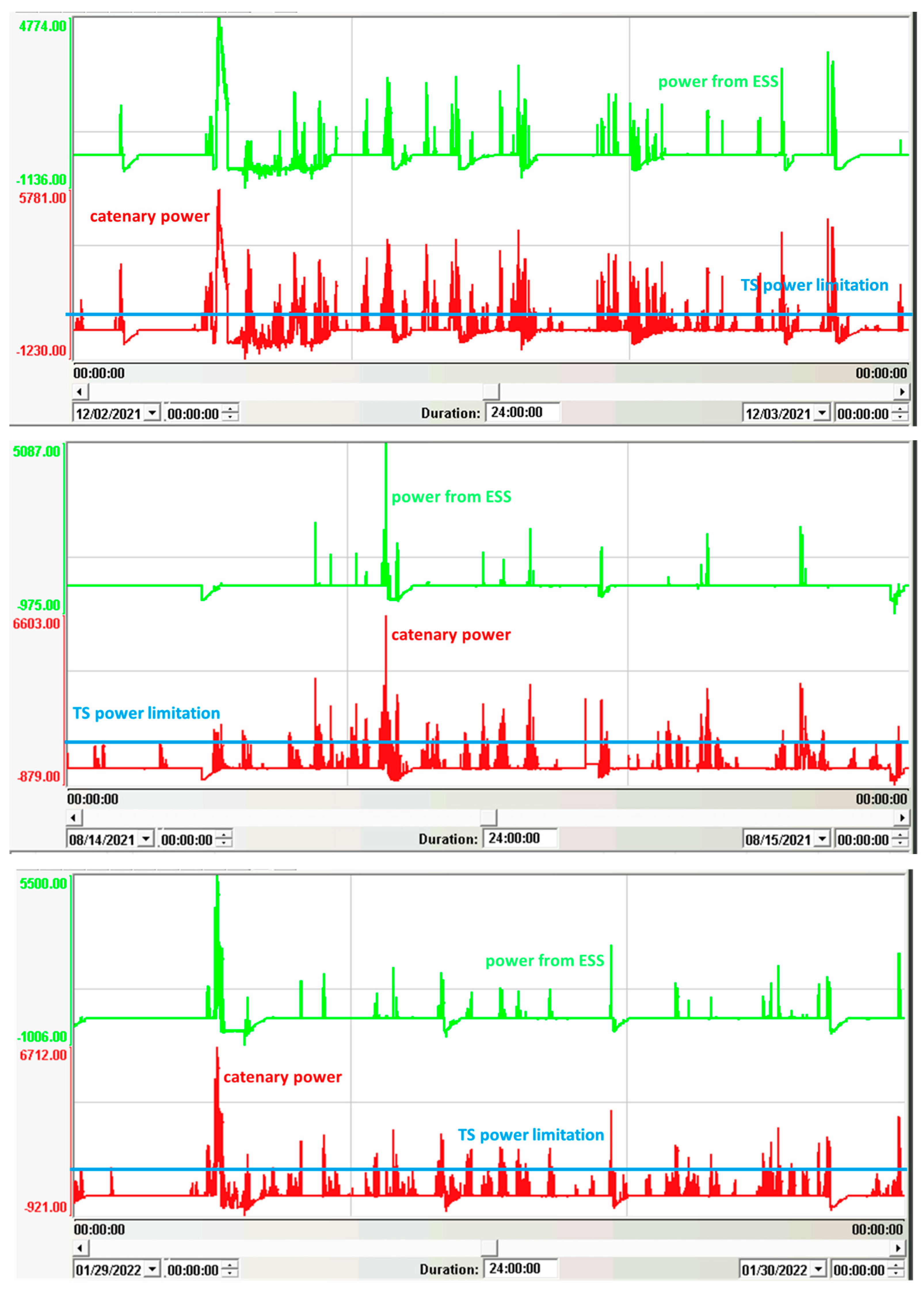
Figure 14 shows three exemplary curves describing the work of the battery energy storage system and the loads on the traction substation. The upper graph shows the power associated with the operation of the battery storage system (positive values are associated with the process of discharging the storage system and negative values with the process of charging it), and the lower graph shows the power curve from the traction substation side.
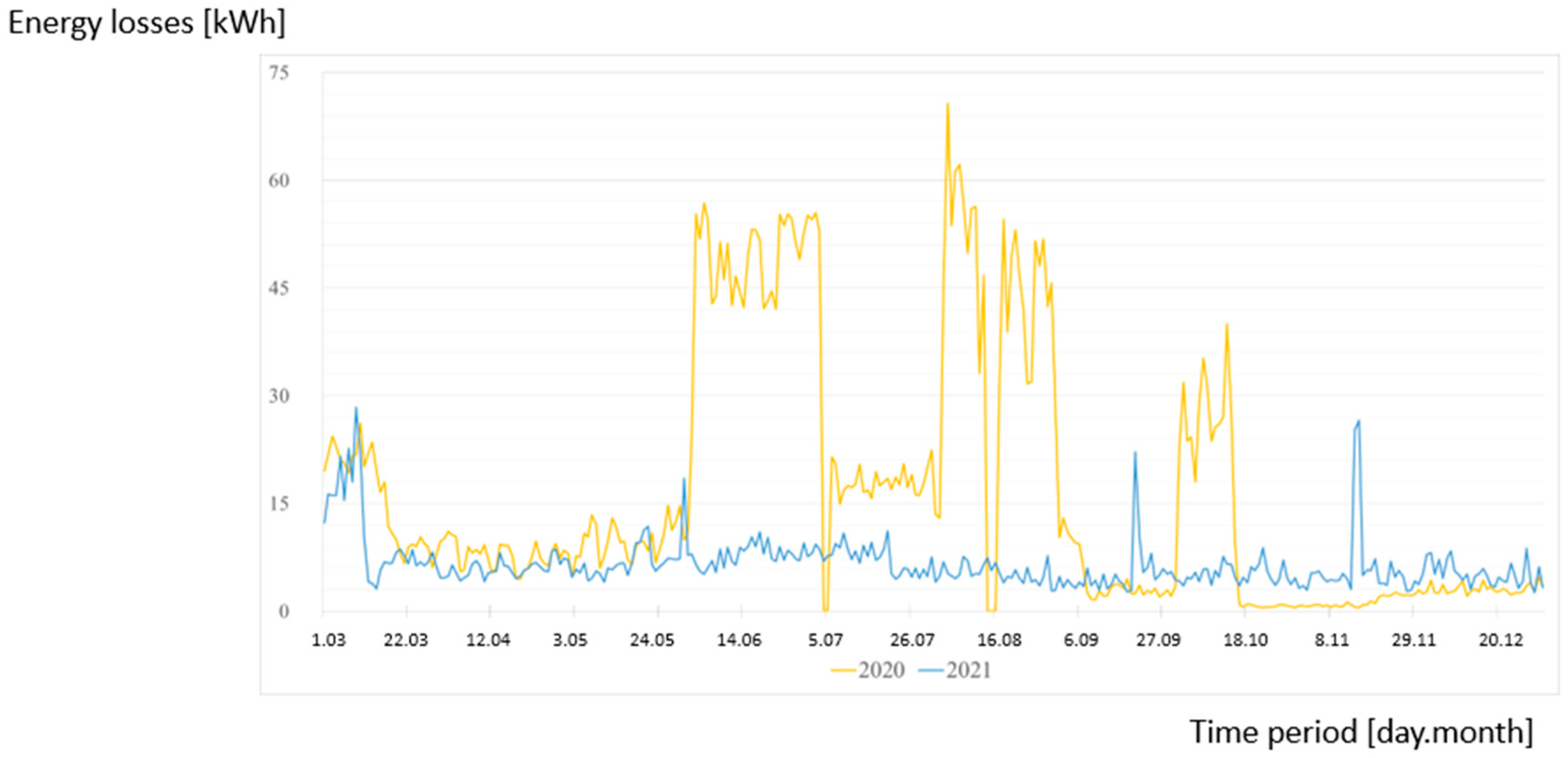
Figure 15 shows the comparison of energy losses (in kWh) in Garbce Zmigrod station supply lines in the period from March to December in 2020 and 2021.
It is clearly visible that, thanks to the battery energy storage system, losses in the supply lines have been reduced. The reduction in energy losses is nearly 60%.
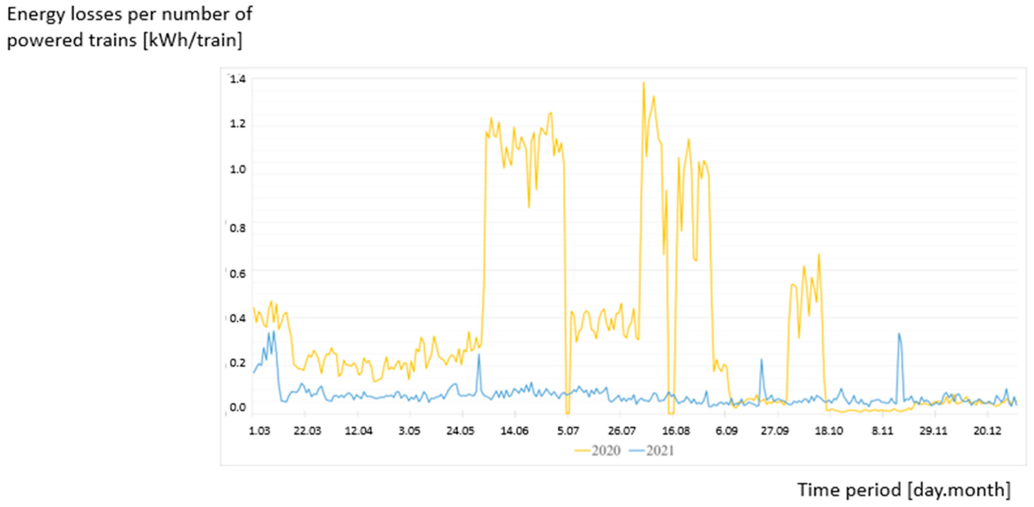
Figure 16 shows the comparison of energy losses in Garbce Zmigrod substation supply lines depending on the number of powered trains (in kWh/train) in the period from March to December in 2020 and 2021.
The reduction in energy losses per powered train is nearly 78%.
The battery energy storage system in Garbce Zmogrod station is a pioneering installation, being one of the first globally to work with a 3 kV DC traction network directly. Its direct DC connection helps reduce energy losses by eliminating the need for DC/AC/DC conversion. Direct connection to the 3 kV DC bus certainly reduces the number of conversions, increases efficiency, enables the immediate absorption of braking energy, and eliminates AC harmonics, reducing investment costs and peak power charges.
The prototype installation has a power of 5.5 MW and a usable capacity of approximately 1.8 MWh (guaranteed 1.2 MWh after 10 years), with a lifespan of at least 15 years. The primary objective of this system is to reduce the peak load on the traction substation caused by railway traffic. This, in turn, leads to a reduction in the contracted power of the facility and the average 15 min power used for billing purposes. When a train operates on the track served by the substation, the energy storage system quickly discharges, providing the necessary power. This significantly lowers the power drawn from the national power system, enabling a substantial decrease in the peak contracted power of the traction substation without limiting the amount or quality of distributed energy. The implementation of the battery energy storage system also results in an improvement in the stability of the DC voltage. This enhanced stability can potentially allow for an increase in railway traffic and the volume of distributed energy without requiring an increase in the contracted power.
Furthermore, it is expected to reduce the impact of individual traction substations on the supplying distribution networks by minimizing power fluctuations and peak demands. This can also be used to provide commercial system services through temporary intentional power reduction on demand. The operation of the battery energy storage system has led to a decrease in both the maximum power of the traction substation and the average 15 min power (contracted power). Considering the dynamics of charging and discharging, it has been possible to reduce the contracted power from 3.6 MW to a range of 1.5–2.0 MW for optimal performance. The maximum value of the charging power limitation of the battery energy storage system was equal to 0.5 MW. Utilizing the battery energy storage system has also lowered energy losses in the power lines supplying the traction substation. This is a consequence of the reduced amount of electrical power delivered, as lower power corresponds to lower current intensity, which is a key factor in energy loss. The Garbce Zmigrod site is also becoming an experimental microgrid with the addition of a photovoltaic farm and a hydrogen energy storage system. This innovative setup will directly integrate renewable generation with energy storage to support the traction network. The PV farm primarily powers the traction energy storage and directly supplies the traction network, while excess energy will be used for the substation’s own needs. The hydrogen storage system uses surplus PV energy to produce hydrogen via electrolysis, which will be stored and subsequently used in fuel cells to power the substation when needed, potentially also serving as fuel for railway vehicles in the future. This microgrid initiative at the Garbce Zmigrod site is envisioned as a foundation for a modern system capable of integrating local energy consumers and producers.


