Article

Quarter-Hourly Power Load Forecasting Based on a Hybrid CNN-BiLSTM-Attention Model with CEEMDAN, K-Means, and VMD

1
Guangzhou Institute of Energy Conversion, Chinese Academy of Sciences, Guangzhou 510640, China
2
School of Energy Science and Engineering, University of Science and Technology of China, Hefei 230026, China
*
Authors to whom correspondence should be addressed.
Energies 2025, 18(11), 2675; https://doi.org/10.3390/en18112675
Submission received: 22 April 2025 / Revised: 13 May 2025 / Accepted: 19 May 2025 / Published: 22 May 2025

Abstract

:
Accurate long-term power load forecasting in the grid is crucial for supply–demand balance analysis in new power systems. It helps to identify potential power market risks and uncertainties in advance, thereby enhancing the stability and efficiency of power systems. Given the temporal and nonlinear features of power load, this paper proposes a hybrid load-forecasting model using attention mechanisms, CNN, and BiLSTM. Historical load data are processed via CEEMDAN, K-means clustering, and VMD for significant regularity and uncertainty feature extraction. The CNN layer extracts features from climate and date inputs, while BiLSTM captures short- and long-term dependencies from both forward and backward directions. Attention mechanisms enhance key information. This approach is applied for seasonal load forecasting. Several comparative experiments show the proposed model’s high accuracy, with MAPE values of 1.41%, 1.25%, 1.08% and 1.67% for the four seasons. It outperforms other methods, with improvements of 0.25–2.53 GWh2 in MSE, 0.15–0.1 GWh in RMSE, 0.1–0.74 GWh in MAE and 0.22–1.40% in MAPE. Furthermore, the effectiveness of the data processing method and the impact of training data volume on forecasting accuracy are analyzed. The results indicate that decomposing and clustering historical load data, along with large-scale data training, can both boost forecasting accuracy.

1. Introduction

With the transformation of the global energy structure and the advancement of smart grid construction, power load forecasting is encountering new opportunities and challenges. As a core component of the energy management system, accurate load forecasting is crucial for building a new power system. It plays an irreplaceable role in achieving efficient energy dispatching, reducing operational costs, and ensuring power grid stability [1]. Especially against the backdrop of the continuous increase in the proportion of renewable energy, power load forecasting has become crucial for anticipating grid supply–demand balance and alleviating the volatility from intermittent energy integration [2]. It also plays an indispensable role in energy sector development and policy formulation [3].
Focusing on temporal and nonlinear characteristics, power load forecasting models are generally categorized into two types. The first is time-series analysis, which includes linear regression [4], exponential smoothing [5], Kalman filtering [6], multiple linear regression [7,8], Fourier expansion models [9], and autoregressive integral moving average (ARIMA) models [10], etc. Time-series analysis uses past and current load values from stochastic time series to predict future loads, considering temporal relationships in the data but having limited predictive power for nonlinear relationships. The second type is machine learning methods, such as BP neural networks [11,12], grey projection [13], and random forests [14]. Time-series analysis uses past and current load values from stochastic time series to predict future loads, considering temporal relationships in the data but having limited predictive power for nonlinear relationships. The second type is machine learning methods, such as BP neural networks [15,16].
The long short-term memory (LSTM) network, effective in nonlinear tasks like language modeling [17], machine translation [18], and speech recognition [19], is increasingly used in load forecasting. It handles temporal and nonlinear data relationships and outperforms traditional methods by capturing long-term dependencies in power data [20,21]. This makes LSTM suitable for addressing the high volatility and uncertainty in power loads, which is crucial as renewable energy penetration increases [22]. However, it struggles to uncover useful information and relationships in non-continuous data [23].
Hybrid architectures combining convolutional neural networks (CNNs) and LSTM models are gaining attention. They integrate CNNs’ spatial feature extraction with LSTMs’ temporal dependency modeling, enabling the handling of both spatial and temporal features. Tae-Young Kim et al. [15] and He et al. [24] show CNN-LSTM networks can effectively extract complex energy consumption features. Bouktif Salah et al. improved LSTM model accuracy by 28% in French grid load forecasting by introducing spatial correlation indicators [21]. Song Jiancai et al. used MAPE as the main evaluation index in regional heating load forecasting, keeping MAPE within 3.1–4.1% with their CNN-LSTM model [25]. Sekhar Charan et al. developed the GWO-CNN-BiLSTM model for weekly load forecasting with multi-metric optimization [26].
Recent studies indicate that hybrid neural network models optimized by attention mechanisms can significantly enhance prediction accuracy and interpretability [27], thus providing novel technical approaches for addressing load mutations. Others developed the CNN-LSTM-A model, which refines LSTM output weights through attention mechanisms, leading to marked improvements in accuracy [16]. Shengdong Du et al. introduced a temporal attention encoder–decoder model. This model employs bidirectional LSTM (BiLSTM) and attention mechanisms to capture long-term dependencies in multivariate time series [28]. Zhou Ning et al. [29] verified that the CNN-LSTM-attention model is superior to LSTM, GRU, CNN-LSTM, CNN-LSTM with autoencoder and parallel CNN-LSTM attention models in predicting fluctuating data.
Despite these advancements, power load forecasting still faces several challenges. The efficiency of deep learning models remains highly dependent on the quality and quantity of historical data. Nivethitha Somu et al. observed that while deep learning frameworks like CNN-LSTM can effectively capture spatiotemporal dependencies in energy consumption, their accuracy is constrained by the sampling frequency and completeness of input data [30]. Despite these advancements, power load forecasting still faces several challenges. The efficiency of deep learning models remains highly dependent on the quality and quantity of historical data. Nivethitha Somu et al. observed that while deep learning frameworks like CNN-LSTM can effectively capture spatiotemporal dependencies in energy consumption, their accuracy is constrained by the sampling frequency and completeness of input data. Lingling Lv et al. utilized Variational Mode Decomposition (VMD) to decompose load data into intrinsic mode functions across different scales [31]. Aksan, F. et al. discovered that the combined model of VMD-CNN-GRU shows good predictive performance under seasonal conditions [32]. Bixuan Gao et al. proposed a CEEMDAN (Complete Ensemble Empirical Mode Decomposition with Adaptive Noise)-CNN-LSTM model designed for feature alignment in historical data [33].
From a temporal perspective, power load forecasting is divided into short-term and long-term categories [3,34]. As the proportion of renewable energy in power systems increases, long-term load forecasting becomes increasingly critical. It plays a key role in effective renewable energy integration, determining a reasonable access scale and distribution, and assessing potential risks in power markets. This paper introduces a data processing method that combines CEEMDAN, K-Means, and VMD. This method is applied to historical power load data from Guangzhou’s power grid, aiming to reduce noise and extract salient features. CEEMDAN decomposes historical data into multiple frequency components. Sample entropy and K-means are utilized successively to evaluate and cluster these components’ regularity and uncertainty. VDM is utilized to further extract the modal components clusters with low frequency and low sample entropy. In this way, the significant regularity of historical data in terms of seasonal, weekly and holiday characteristics and the uncertainty in terms of hourly randomness and diurnal variation characteristics are extracted, which is more conducive to the model’s capturing of data characteristics. This study also proposes a CNN-BiLSTM model based on attention mechanisms for long-term load forecasting. The CNN layers extract spatial features from training data, the BiLSTM layers capture short- and long-term dependencies in sequential data from both directions, and the attention mechanism enhances key information impacts. The proposed model’s performance is compared with those of other deep learning methods, showing its effectiveness in improving forecasting accuracy across different seasons.
The main contributions of this paper are the following: (1) proposing a combined data processing approach, (2) developing the CNN-BiLSTM-attention model, (3) comparing the model’s effectiveness with other methods, (4) validating the data processing method’s effectiveness in improving forecasting accuracy, and (5) by grouping the training and test sets in different proportions, the impact of data quantity on model feature learning is further studied.
The rest of this paper is organized as follows: Section 2 details the data processing methods and steps. Section 3 presents the CNN-BiLSTM-attention model. Section 4 discusses the case study results. Finally, Section 5 summarizes the research.

2. Data Processing

This study uses the hourly historical power load data of Guangzhou from 2020, with a total of 8784 data points. The task of this study is to improve the robustness and accuracy of power load forecasting. Due to the influence of day–night differences and season, the power load shows multi-frequency characteristics. At the same time, user behavior and environmental factors also cause the power load to present uncertainty. Using CEEMDAN or VMD to decompose the data into simple frequency features and predict the modal decomposition is an effective method to ensure the function fitting and subsequent convergence of the prediction model. By introducing adaptive noise to reduce the modal effect, CEEMDAN can improve the accuracy of nonlinear and non-stationary signal decomposition. VMD has a good anti-noise ability and can effectively capture the frequency characteristics of signals. The combination of CEEMDAN and VMD can decompose the load sequence into trend terms and multiple random fluctuation terms, which can further reduce the complexity of the sequence, enhance the robustness of the data, and better preserve the main characteristics of the signal.

2.1. Complete Ensemble Empirical Mode Decomposition Adaptive Noise (CEEMDAN)

CEEMDAN is a signal processing technique proposed by Torres et al. in 2011 [35]. By adding white noise step by step, averaging step by step and introducing adaptive noise, CEEMDAN can effectively solve the common mode aliasing problem of traditional empirical mode decomposition (EMD) when dealing with nonlinear and non-stationary signals. CEEMDAN processes signals into multiple Intrinsic Mode Functions (IMFs) as follows:
(1)
Add Gaussian white noise to the original signal to initialize the original signal,
Y n ( t ) = Y ( t ) + ε 0 λ n ( t ) , n = 1 , 2 , …… , N
where ε 0 is the weight coefficient of Gaussian white noise; λ n ( t ) is the Gaussian white noise at the n-th processing; N represents the number of realizations.
(2)
Perform the EMD decomposition on all preprocessing sequences, and then the first IMF I m f ¯ 1 ( t ) is calculated by averaging the decomposed components,
I m f ¯ 1 ( t ) = 1 N 1 N I M F 1 i ( t )
r 1 ( t ) = Y ( t ) I m f 1 ¯ ( t )
where r 1 ( t ) is the first residual.
(3)
Gaussian white noise is added to the residual sequence to construct a new sequence, r 1 ( t ) + ε 1 E M D 1 ( λ n ( t ) ) . After the further EMD decomposition of this sequence, the second IMF I m f ¯ 2 ( t ) component and residual r 2 ( t ) are obtained by calculating its mean value,
I m f ¯ 2 ( t ) = 1 N 1 N E M D 1 ( r 1 ( t ) + ε 1 E M D 1 ( λ n ( t ) ) )
r 2 ( t ) = r 1 ( t ) I m f 2 ¯ ( t )
(4)
The residual of stage m-th is shown as
r m ( t ) = r m 1 ( t ) I m f m ¯ ( t )
(5)
Performing the EMD decomposition on the m + 1-th sequence r m ( t ) + ε m E M D m ( λ n ( t ) ) to obtain the m + 1-th IMF I m f ¯ m + 1 ( t ) yields
I m f ¯ m + 1 ( t ) = 1 N 1 N E M D 1 ( r m ( t ) + ε m E M D m ( λ n ( t ) ) )
where E M D m ( ) is the m-th IMF model obtained by EMD decomposition.
(6)
Repeat the above steps until the decomposition satisfies the stop condition, and the final residual sequence is
t = 0 T r m 1 ( t ) r m ( t ) 2 r m 1 2 S D m
where T represents the length of the sequence Y n ( t ) ; r m ( t ) is the sequence after m-th decomposition, and the experience value S D m is set to 0.2 [36].
Through the above steps, the Guangzhou historical power load sequence is decomposed into 14 IMFs, which includes high frequency and low frequency, as shown in the Figure 1. IMF1 to IMF3 belong to high-frequency modes, mirroring short-term fluctuations and noise in the power load sequence, likely derived from sudden load changes. IMF4 to IMF6 belong to medium-frequency modes, contain multiple relatively stable frequencies, and show regular fluctuations of power load on a medium timescale. The rest are low-frequency IMFs, reflecting long-term trends and slow variations of power load, like gradual fluctuations and overall upward or downward trends caused by factors such as seasonality. While low-frequency IMFs have relatively few frequency components, their energy share is higher.

2.2. K-Means Clustering

This study applies CEEMDAN to decompose the original complex signal into multiple modal components with different frequencies and characteristics, and effectively extract different levels of information in the signal. K-means is a clustering algorithm that can divide data points into K clusters. The data points within each cluster are as similar as possible, and the data points between different clusters are as different as possible. To classify the regular characteristics of the IMFs, the regularity and uncertainty of the 14 IMFs in Figure 1 are first evaluated using the sample entropy method [37]. Then, we perform K-means clustering on the sample entropy values to classify the IMFs and reduce dimensionality. Combining CEEMDAN and K-means to process the data can provide better input for subsequent analysis and modeling, and improve the robustness and generalization ability of the model. The core of K-means is to optimize clustering results by minimizing the Within-Cluster Sum of Squares (WCSS). The objective function of K-means clustering is defined as
J = j = 1 K i = 1 n 1 x i C l u j d ( x i , c l u j ) 2
where K is the number of predefined clusters; C l u j presents the k-th cluster; x i is the j-th data point; c l u j is the center of the k-th cluster; 1 x i C l u j represents the indicator function, which is 1 when belonging to a cluster and 0 otherwise. d ( x i , c l u j ) represents the distance between x i and c l u j , which is used to measure the similarity between the data points, usually using the squared Euclidean distance,
d ( x i , c l u j ) = k = 1 d ( x i , k c l u j , k ) 2
The clustering steps of K-means are as follows:
(1)
Initialization. Randomly select K data points as the initial cluster centers c l u 1 , c l u 2 ,…, c l u k ;
(2)
Assign data points to the nearest cluster. For each x i , calculate its distance to all cluster centers and assign it to the nearest cluster;
(2)
Update cluster center. For each C l u j , update the cluster centroid by calculating the mean of all x i in the cluster,
c l u j = 1 C l u j x i C l u j x i
where C l u j is the number of x i in C l u j .
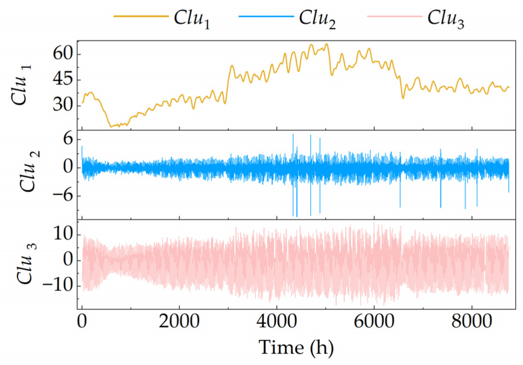
The sample entropy values of 14 IMFs are shown in Table 1. A smaller sample entropy value indicates that the IMF has strong regularity or predictability. The Silhouette Coefficient and Elbow methods are combined to select the optimal K value. In Figure 2a, the Silhouette Coefficient exceeds 0.9 for K = 2 and K = 3, indicating well-separated clusters. Figure 2b shows that when K = 3, the Sum of Squared Errors (SSE) still shows a rapid decline. However, as the K value continues to increase, the decline in SSE sharply decreases and the curve becomes flat. Based on these findings, K = 3 is chosen as the optimal value. Figure 2c presents the clustering results for the sample entropy of the 14 IMFs, where the cluster centers are 0.0704, 0.6501 and 1.7713, respectively.
By adding up the IMFs contained in each cluster individually, the 14 IMFs in Figure 1 are divided into three clusters as shown in Figure 3. Clu1 is the largest cluster with an aggregation of eight IMFs. Clu2 and Clu3 each contain three IMFs.

2.3. Variational Mode Decomposition (VMD)

Finally, VMD is used to further decompose the Clu1 in Figure 2 to effectively extract the key features of the signal. VMD is a non-recursive signal decomposition method based on variational theory proposed by Konstantin Dragomiretskiy and Dominique Zosso in 2014 [38], which has excellent performance in the decomposition of low-frequency components. The VMD algorithm shows little influence on the initial conditions and has strong robustness. The central idea of VMD is to assume that the original signal u ( t ) can be decomposed into the sum of k IMFs, with each u k ( t ) having a specific central frequency ω t and bandwidth k . The u k ( t ) can be found by minimizing the total k ,
min u k , ω k k = 1 K t δ ( t ) + j π t u k ( t ) e j ω k t 2 2
s . t .   k = 1 K u k ( t ) = u ( t )
where t represents the differential operation; represents the convolution operation; δ ( t ) is the Dirac function; j is an imaginary unit; e j ω k t is the modulation operation.
VMD transforms the constrained variational problem into an unconstrained variational problem by using the augmented Lagrange function. The extended Lagrange expression is as follows:
L ( u k , ω k , λ ) = α k = 1 K t δ ( t ) + j π t u k ( t ) e j w k t 2 2 + u ( t ) k = 1 K u k ( t ) 2 2 + λ , u ( t ) k = 1 K u k ( t )
where α is the quadratic penalty factor; λ is the Lagrange multiplication operator.
Iterative optimization is performed by alternating direction multiplier method (ADMM), updating u ^ k n + 1 ( ω ) and ω k n + 1 for all ω 0 :
u ^ k n + 1 ( ω ) = f ^ ( ω ) i k u ^ i n ( ω ) + λ ^ n ( ω ) / 2 1 + 2 α ( ω k n ω ) 2
ω k n + 1 = ω u ^ k n + 1 ( ω ) 2 d ω u ^ k n + 1 ( ω ) 2 d ω
The λ ^ n + 1 ( ω ) can be updated as
λ ^ n + 1 ( ω ) = λ ^ n ( ω ) + τ u ^ ( ω ) k = 1 K u ^ k n + 1 ( ω )
where f ^ is the frequency domain representation of u ( t ) ; u ^ k is the frequency domain representation of the IMF; ω k n is the estimated value of the center frequency of the k-th mode at the n-th iteration; λ ^ n ( ω ) is the Fourier transform of the Lagrange multiplier at the nth iteration; τ represents the noise tolerance.
The detailed decomposition steps of VMD for u ( t ) are as follows:
(1)
Initialize u ( t ) , ω t and λ 1 ;
(2)
Set n = n + 1;
(3)
k = k + 1, and for all ω 0 , update u ^ k n + 1 ( ω ) and ω k n + 1 ;
(4)
Update λ ^ n + 1 ( ω ) ;
(5)
Repeat steps (2)–(4) until the following stop conditions are met—
k = 1 K u ^ k n + 1 u ^ k n 2 2 u ^ k n 2 2 < γ
As shown in Figure 3, Clu1 contains multiple low-frequency and low-sample-entropy IMFs with significant regularity. Considering that the long-term characteristics selected by the model include week and holidays, and the power load has strong seasonal characteristics, the initial decomposition layer number of VMD is set to 3 in order to capture week, holiday, and seasonal features. This operation is carried out by using the VMD function in Octave software 10.1.0. The penalty factor alpha is set to 2500 and the convergence threshold is set to 1 × 10⁻⁶.
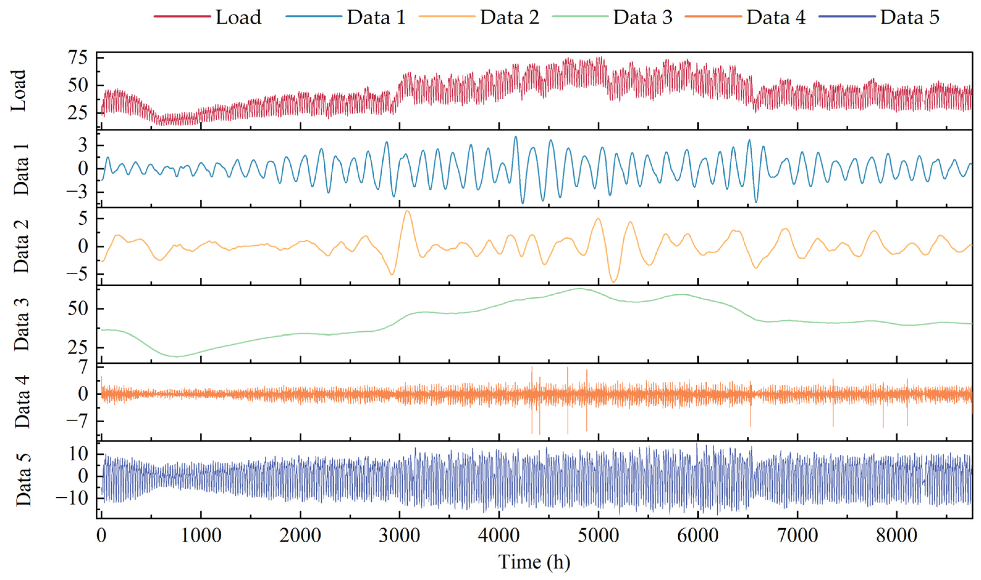
Through the above steps, Clu1 is decomposed into three IMFs by the VMD algorithm. Combined with Clu2 and Clu3, the power load sequence is finally decomposed into five components, as shown in Figure 4.
Figure 4 shows that after CEEMDAN, K-means and VMD processing, the week characteristics (Data 1), holiday characteristics (Data 2) and seasonal characteristics (Data 3) of the power load sequence are extracted. Load uncertainty is divided into hourly random uncertainty (Data 4) and diurnal uncertainty (Data 5).

2.4. Feature Selection and Normalization

In this work, we study the hourly power load sequence of Guangzhou. We select the most commonly used features in the load forecasting literature to obtain attributes from the data. Guangzhou is a subtropical monsoon climate, which has a high demand for air conditioning cooling in summer and heating in winter. Thus, temperature is chosen as a feature. The above power load decomposition results show that the power load has obvious characteristics related to week, holiday and season. One hour in a day (values from 1 to 24), one day in a week (values from 1 to 7), and holiday indicators (0, 1 and 2 represent non-holidays, common legal holidays, and Spring Festival, respectively) are also considered as features. Through the above assignment, the temperature, date and other features of 2020 are composed into a 4-dimensional feature data matrix.
As can be seen from Figure 3, the power load in Guangzhou has obvious seasonal characteristics. Therefore, this paper separately models the four seasons to improve the prediction accuracy. The feature data matrix and each load IMF in Figure 3 are divided into four seasons, respectively: spring, summer, autumn and winter. Then, the feature matrices of each season and each load IMF are combined to form the model input matrix. Thus, the forecast model for each season contains five 5-dimensional input matrices. For each season, each input matrix is modeled in turn, and then the prediction performance is evaluated after summing the forecast results. Max–min scaling is used to normalize input data to eliminate dimensional effects between data features,
X n o r m = X X min X max X min
where X n o r m is the data after normalization; X is the input raw data set; X min and X max are the minimum and maximum values of the original data, respectively.

3. Methods

CNN demonstrates a robust capability in spatial feature extraction. LSTM is particularly effective in extracting sequential patterns and capturing both short-term and long-term dependencies of sequence data. The integration of CNN and LSTM has been proven to be highly effective in capturing spatial correlations and temporal trends, making it a powerful approach for complex sequence data analysis. BiLSTM can simultaneously process sequence data in both forward and backward directions, significantly enhancing the accuracy of sequence modeling tasks. By incorporating an attention mechanism and dynamically optimizing the output weights of BiLSTM through weight allocation, the influence of key information can be enhanced, while addressing the limitations of BiLSTM in processing long sequence data. Therefore, a hybrid model leveraging the synergistic advantages of CNN, BiLSTM, and attention mechanisms is expected to improve the accuracy of load prediction. This section provides a detailed description of the components of the CNN-BiLSTM-attention architecture.

3.1. Convolutional Neural Network (CNN)

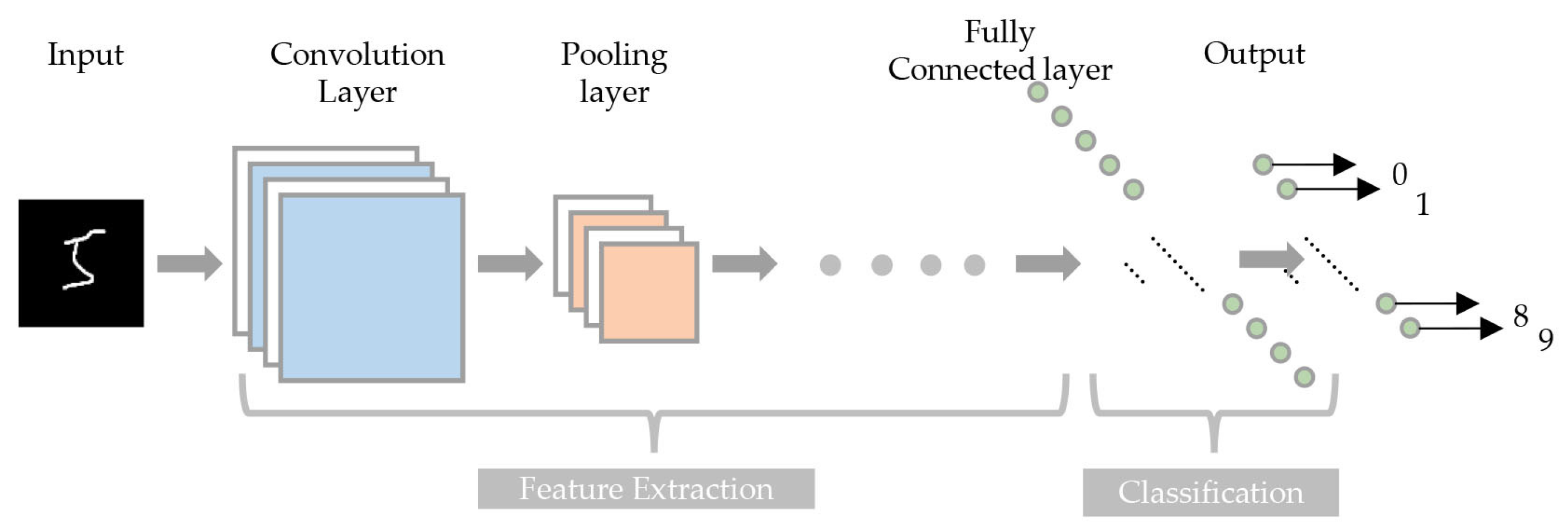
Introduced by [39], CNN is a DNN model primarily inspired by biological processes [40]. CNN serves as a powerful tool for automatic feature extraction and expression, capable of achieving arbitrary function mapping from input to output. While CNN is widely used in image vision tasks, its applications have also expanded to time-based serial data, as evidenced by recent studies [41,42]. CNNs typically use multiple building blocks such as convolutional, pooling, and fully connected layers to learn the spatial hierarchy of features (as shown in Figure 5). The convolutional layer extracts input features by performing multi-depth convolutions with kernels and applying nonlinear mapping via activation functions, allowing the network to focus on local regions. The pooling layer summarizes features from convolutions, reducing data dimensionality through max or average pooling to minimize computations. Finally, the fully connected layer, integrated as a BP neural network at the network’s base, merges pooled features to learn global input characteristics, and generates the output [43].

3.2. Bidirectional Long-Term Memory Network (BiLSTM)

Recurrent Neural Networks (RNNs) are widely used for analyzing and predicting sequential data. However, the vanishing gradient problem limits their ability to capture long-term dependencies [44], while the exploding gradient problem can lead to model instability and failure to converge. To address these issues, Sepp Hochreiter and Jürgen Schmidhuber proposed LSTM networks in 1997. Subsequently, Felix Gers and colleagues introduced the forget gate mechanism to further enhance LSTM’s capabilities [45]. The improved LSTM architecture leverages a gating mechanism—comprising the input gate, forget gate, and output gate—along with a cell state update and self-connected memory cells to capture complex temporal dependencies in both long and short time-series data. This design aims to overcome the limitations of traditional RNNs, particularly their susceptibility to vanishing and exploding gradients when processing long sequences, as well as their inability to effectively model long-term dependencies.
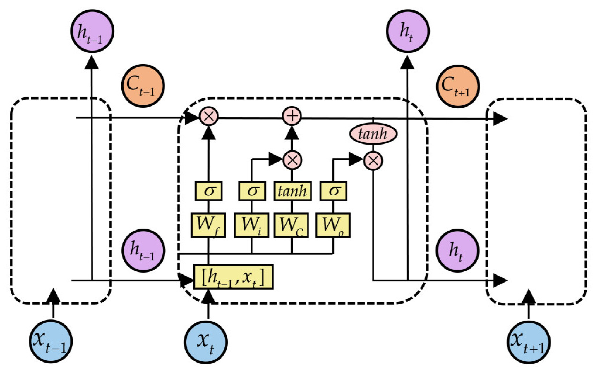
The input gate i t , forget gate f t , and output gate o t regulate the flow of information by determining what to add or remove from the cell state [46,47] (as shown in Figure 6). The memory cell retains temporal state information from both the current and previous time steps. For a given input x t at time step t, the forward computation process of LSTM can be expressed as:
i t = σ ( W i h t 1 , x t + b i )
f t = σ ( W f h t 1 , x t + b f )
o t = σ ( W o h t 1 , x t + b o )
C ^ t = t a n h ( W C h t 1 , x t + b C )
C t = f t C t 1 + i t C ^ t
h t = o t t a n h ( C t )
where σ is the activation function; t a n h denotes hyperbolic tangent activation; W i , W f , W o , W C and b i , b f , b o , b C are the weight matrices and bias of i t , f t , o t and cell state update C ^ t , respectively; C t 1 and C t represent the previous and current cell states, respectively; h t is the hidden state and is updated according to the o t and the updated memory unit state.
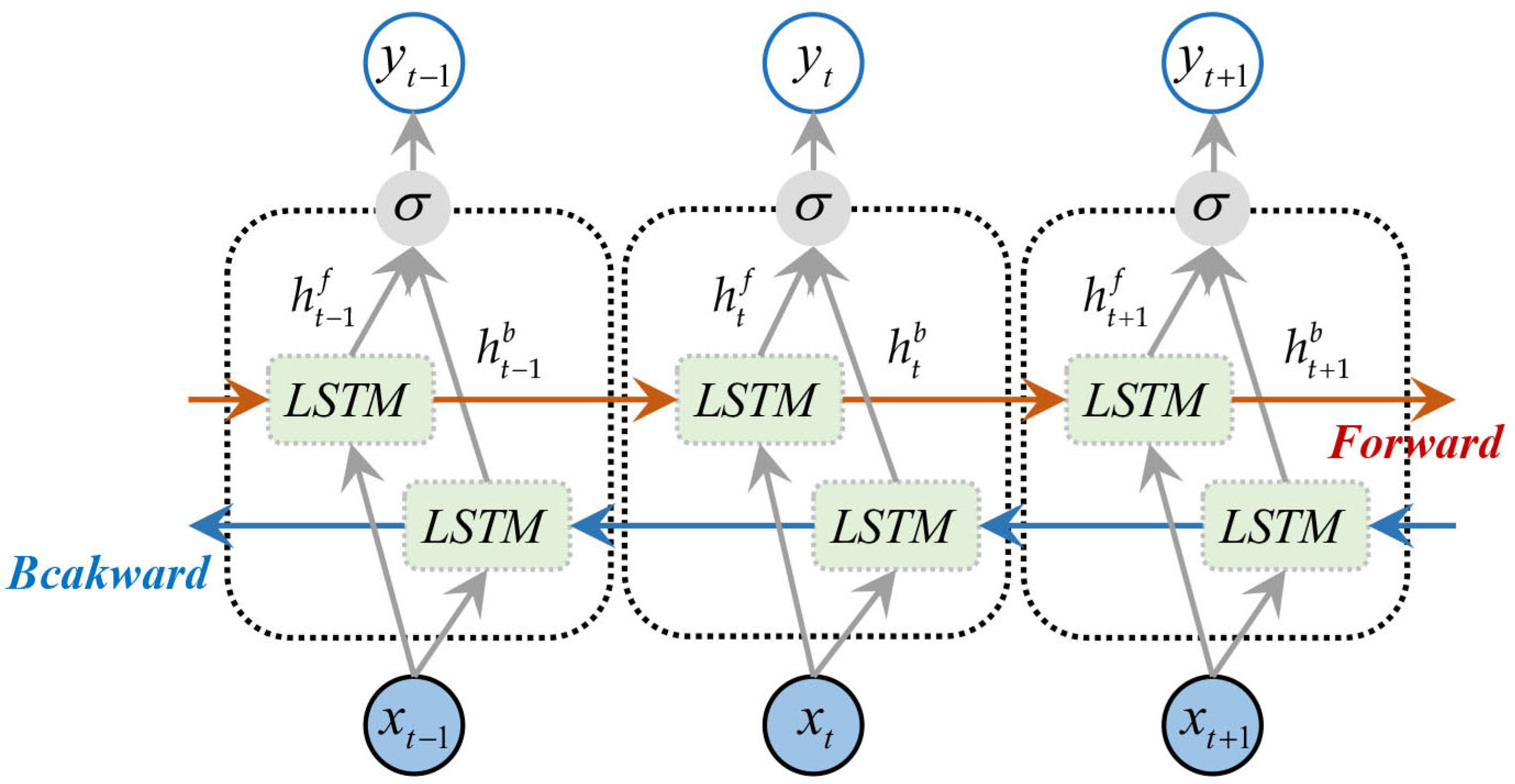
Since inputs in LSTM are processed in a precise temporal order, future information cannot be utilized. It is critical to understand contextual information in many sequence modeling tasks (such as natural language processing and speech recognition). In 2005, Graves proposed combining LSTM with Bidirectional Recurrent Neural Networks (BRNNs) to form BiLSTM [48]. A BiLSTM consists of two LSTM layers: one processes the forward sequence (from the first element to the last), and the other processes the backward sequence (from the last element to the first). The outputs of these two layers are concatenated at each time step or at the end of the sequence, enabling the model to leverage both past and future information and capture contextual relationships more comprehensively. The hidden layer output of the BiLSTM model h t at time step t is
h t = h t f ; h t b
where h t f and h t b are forward and reverse hidden sequences, respectively. Figure 7 depicts the design of BiLSTM prediction. The output is represented by y t .

3.3. Attention Mechanism

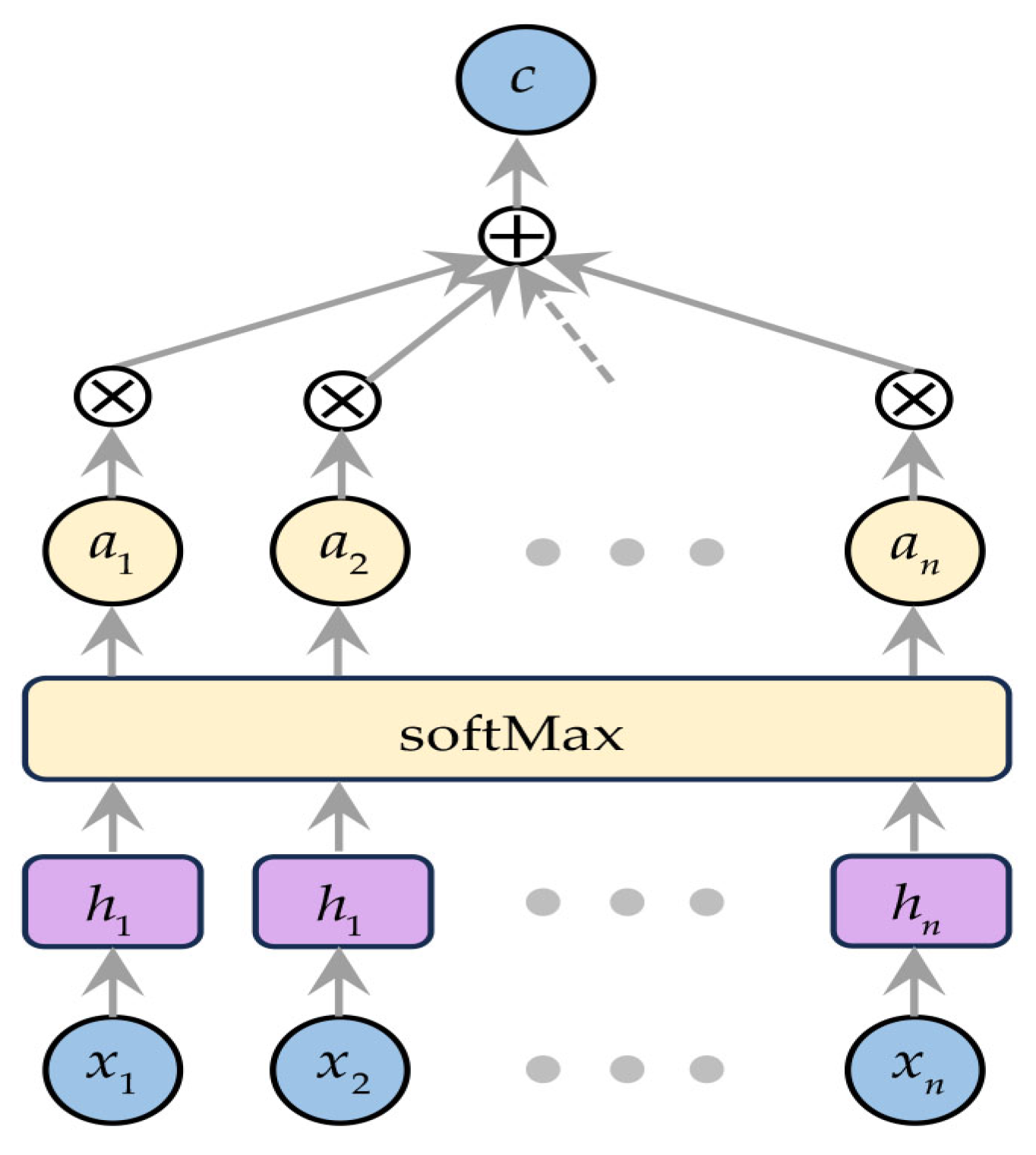
In practical problems, some features are more important than others. For instance, in electricity load forecasting, certain information like weather and day types may be more significant. Traditional neural networks treat all inputs equally, making it hard to focus on key information in the input sequence. Attention mechanisms, inspired by human visual attention, enhance important information in deep neural networks. They assign probabilities to information instead of using random weights, addressing information loss in LSTM and BiLSTM caused by long sequences. The structure of attention models is shown in Figure 8.
The attention mechanism assigns different weights to various inputs to discard irrelevant information, amplify key information and enhance model accuracy. This paper focuses on soft attention mechanisms that emphasize regions or channels. In soft attention, inputs are projected into multiple subspaces, each with different weights that can be learned or preset based on the problem. During each computation, these weights are recalculated to adapt to the current task, suppressing irrelevant features. In Figure 7, a t is the attention weight assigned to the BiLSTM hidden layer output h t ; higher a t values indicate more relevant historical features. The optimized BiLSTM output after attention is denoted as c t . The attention layer weights are computed as follows:
e t = ν T t a n h ( W e h t + b e )
a t = exp ( e t ) j = 0 t exp ( e j )
c t = t = 0 t a t h t
where e t represents the attention scoring function, which quantifies the correlation between the power load at time t and the output vector of the BiLSTM layer; ν T is a learnable vector; b e is the bias in the network training; t a n h is the activation function; e j is the weighted result of the implicit function’s output.

3.4. Proposed Model Architecture

The architecture of the CNN-BiLSTM deep learning framework with an attention mechanism as proposed in this study consists of the following layers: input, CNN, BiLSTM, attention and output. The input layer receives historical load sequences and feature data such as weather, along with preprocessing. A sequence folding layer is inserted between the input and CNN layers to perform convolution independently at each time step.
The CNN is used to extract spatial features from temporal data and consists of a 2D convolution layer, a Rectified Linear Unit (ReLU) layer, and a MaxPooling layer. The 2D convolution layer has a kernel size of [1, 3] and contains 16 filters. The ReLU activation function maintains the nonlinearity of the output and addresses gradient issues. The MaxPooling layer, with a kernel size of [1, 2], reduces the spatial dimensions of the feature maps by a factor of two, lowering feature dimensionality and preventing overfitting. A Batch Normalization (BN) layer is added between the convolutional and ReLU layers to accelerate training and avoid gradient vanishing or explosion. After the MaxPooling layer, a sequence Unfolding Layer is added to restore the output of the convolutional layer to a sequence structure. Finally, a Flatten Layer is used to flatten the sequence data into a one-dimensional vector for connection to the BiLSTM layer.
A BiLSTM layer models dependencies in temporal data, comprising 20 hidden layers and outputting hidden states at the final time step. Its output connects to a self-attention layer, which optimizes the BiLSTM output weights. This enhances important features and suppresses irrelevant ones. The self-attention layer has 40 channels, two heads, and two key and query channels. Before the fully connected layer, a dropout layer randomly deactivates neurons with a 0.1 probability of reducing overfitting. The fully connected layer transforms features into a 1D structure for the output layer to produce final predictions. Parameters of this CNN-BiLSTM-attention prediction model are summarized in Table 2.
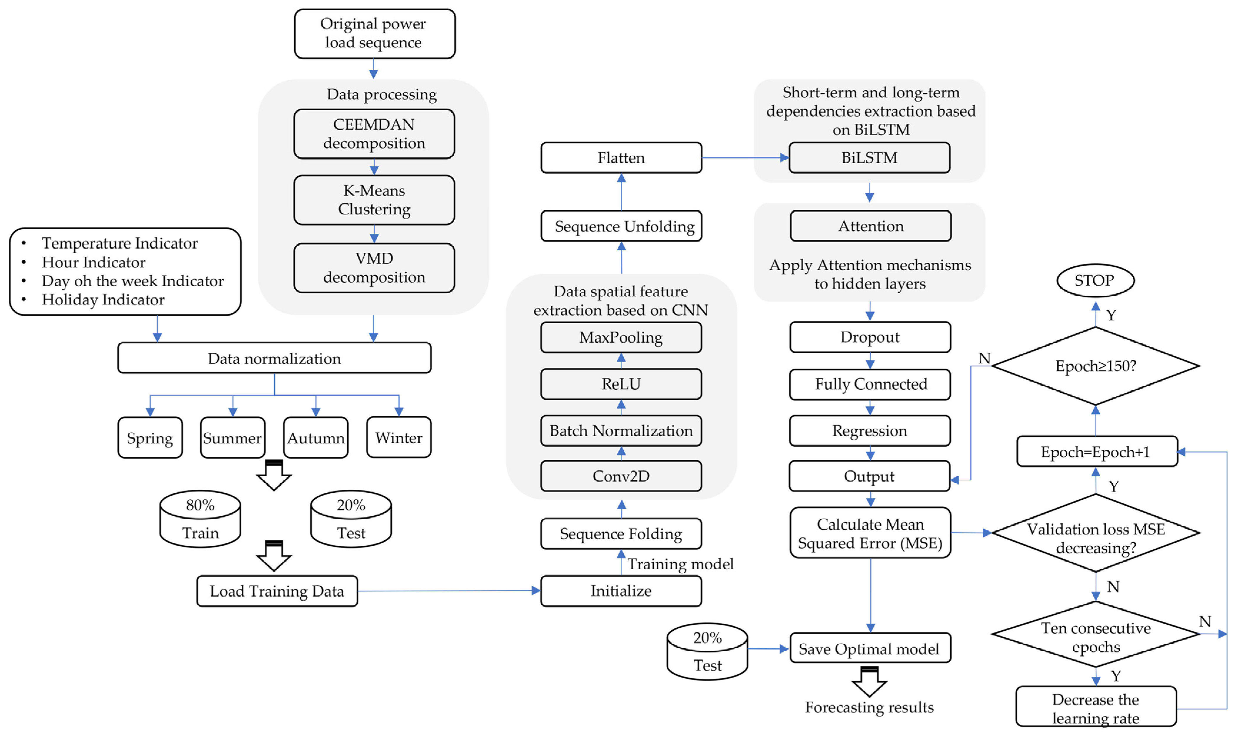
The entire process of the proposed model is shown in Figure 9 and is described in detail as follows:
(1)
Before decomposing the original power load sequence, data organization and cleaning are required to unify the data format and remove abnormal items;
(2)
CEEMDAN is applied to decompose the power load sequence into multiple IMFs with different frequencies and characteristics, removing noise from the historical load data. We then calculate the sample entropy of these IMFs, and K-means clustering is used to classify these sample entropies, extracting more representative features for the dimensionality reduction of each IMF component. VMD is then applied to further decompose the largest cluster from the K-means clustering to more finely extract the main signal characteristics;
(3)
The processed power load IMFs and feature matrices form five 5-dimensional data matrices, which are normalized to eliminate the impacts of different magnitudes on the prediction model;
(4)
The five processed data matrices are divided into four seasons—spring, summer, autumn, and winter. For each season, the training and test datasets are split in a ratio of 4:1;
(5)
The training data are loaded, and the model parameters are initialized. The model is trained using the five sets of training data for each season, monitoring the loss and accuracy during training. If the validation loss decreases, the model is saved with the updated weights, and the epoch count is increased. If the validation loss does not decrease for 10 consecutive epochs, the learning rate is reduced. Training stops when the epoch count reaches 150;
(6)
Finally, the optimal hyperparameter model of the CNN-BiLSTM-attention network obtained from the grid search is saved. This model is then loaded onto the test data for prediction and evaluation to avoid overfitting.

4. Case Study

4.1. Evaluation Index

The prediction accuracy of the model is evaluated using four error metrics. Mean Square Error (MSE) and Mean Absolute Error (MAE) reflect the deviation between predicted and actual values; smaller values indicate higher prediction accuracy. Root Mean Square Error (RMSE) measures the differences between predicted and actual values, with smaller values indicating smaller differences. R2 assesses the goodness of fit of regression models; higher values suggest stronger explanatory power. The formulas for calculating these metrics are
MSE = 1 N i = 1 n ( y true y predict ) 2
MAE = 1 N i = 1 n y true y predict
RMSE = 1 N i = 1 n ( y true y predict ) 2
R 2 = 1 i = 1 n ( y true y predict ) 2 i = 1 n ( y true y true ¯ ) 2
where y predict is the predicted value of the load; y true is the actual value of the load; y true ¯ is the average value of the actual load; N indicates the number of data samples.

4.2. Hyper-Parameter Setting

The input layer of the model receives raw data of an eight-step time series with a dimension of 5 (8 × 5). The hyperparameters of the proposed deep learning framework are set as shown in the Table 3. The solver used is Adam, and the loss function is MSE. The initial learning rate is 0.001. The maximum number of epochs is set to 150.

4.3. Prediction Performance Analysis

4.3.1. Training Process Evaluation

In this study, an hourly prediction model is established to forecast power load using temperature, time features, day-of-week features, and holiday features. The hourly dataset throughout the year is divided into training and test data at an 80% to 20% ratio, respectively. Furthermore, due to the influence of seasons on the accuracy of load forecasting, the dataset is further divided into four seasons.
To validate the superiority and predictive ability of the proposed model, CNN-BiLSTM (C-B), CNN-LSTM (C-L), LSTM-A (L-A), and LSTM (L) are chosen as benchmark models. The proposed model uses the five IMFs data of Guangzhou decomposed and clustered by CEEMDAN, K-means, and VMD algorithms, while the other models uses the original power load data sequence.
The model was run using Python 3.13 software on a computer with an i-7-14700 (28 CPU) processor and 16,384 MB of memory.
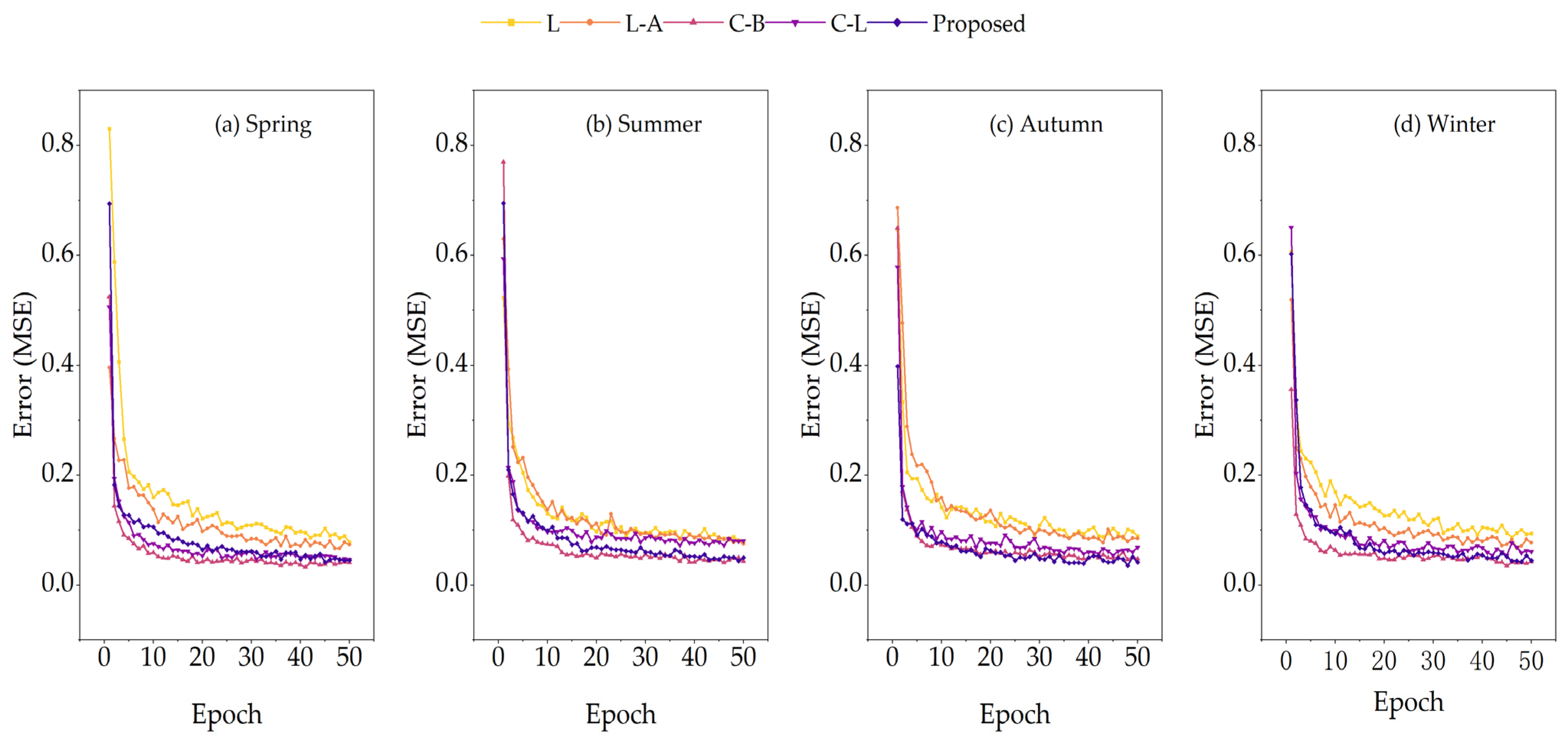
Table 4 and Figure 10, respectively, present the changes and processes of MSE of the five models after 50 iterations. The results show that models with CNN structure converge quickly during the early training stages of four seasons, and adding a BiLSTM structure could further speed up early convergence. L-A and traditional LSTM converge slowly, with no clear convergence after 50 iterations, leading to higher prediction errors than CNN-based models. Figure 10 indicates that after optimizing weight allocation with attention mechanism, L-A converges faster than traditional LSTM in spring and winter, with smaller error values. Overall, the proposed model has good convergence speed and the most stable error distribution.
Table 5 lists the total training time needed by each model to complete four-season forecasting, so as to evaluate the models’ computational efficiency. The proposed model needs to train on five datasets per season, with a total training time of 449 s across the four-season data. On average, it takes 22.5 s for our model to train on each dataset, similar to C-B’s average of 21.25 s, which is a bit higher than C-L’s 19.75 s, and about 2.2 times the training time needed by the L-A Traditional LSTM.

4.3.2. Prediction Effect

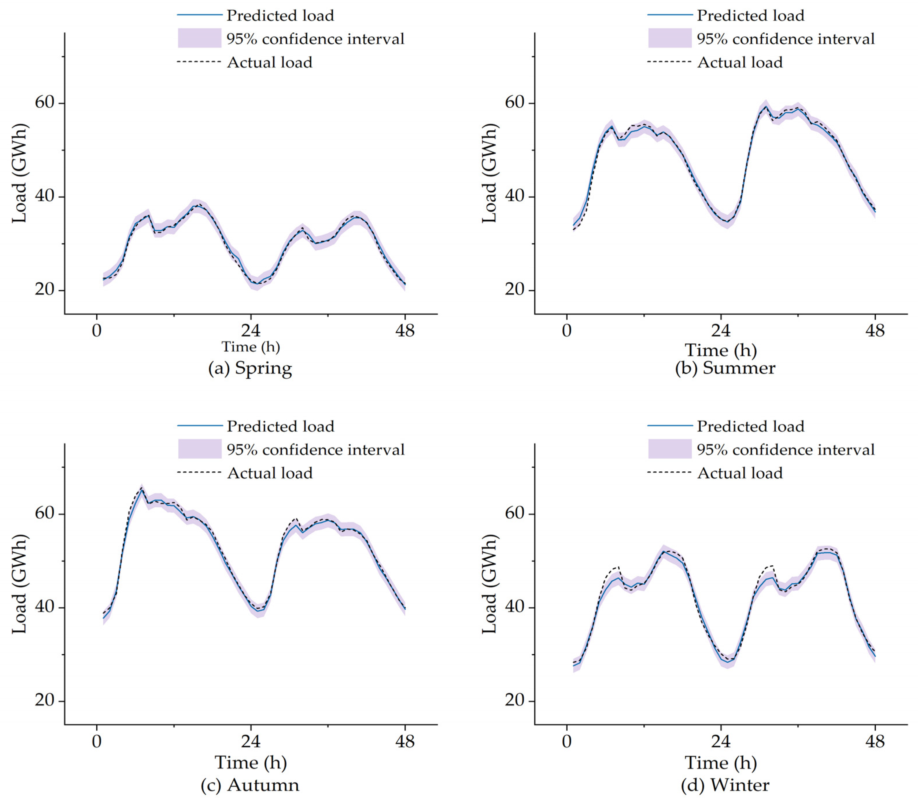
As shown in Figure 11, the proposed model demonstrates good predictive performance in terms of both load levels and trends for the initial 48 h of the test set across the four seasons. Except for winter, the actual values can all fall within the 95% confidence interval of the prediction. This is because the winter testing period coincided with the post-pandemic reopening phase. There was a large-scale commissioning of industries, foreign trade, and infrastructure, leading to a surge in electricity consumption. In the winter test set, two load peaks on several days increased dramatically. Such load distribution trends were absent in the training set. Moreover, such changes in trade were not among the features considered in the proposed model. Therefore, the model did not capture the impact of trade on electricity load during training. Although only four days of peak load predictions deviated from actual values, this was a significant proportion of the 18-day training set. This is also the main reason why all models performed the worst in winter predictions.

4.3.3. Prediction Accuracy

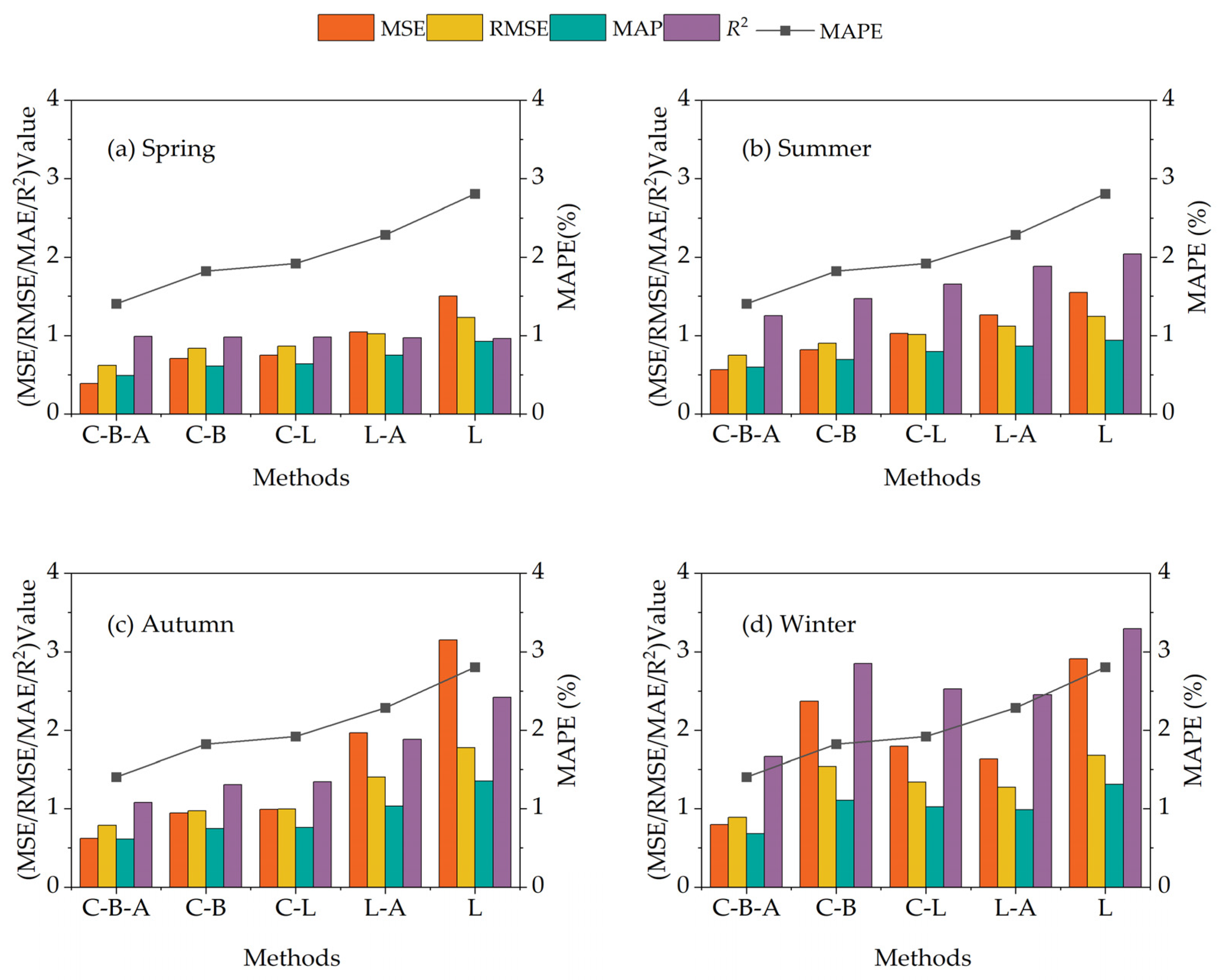
Each model of each season has been evaluated 10 times, and the results with the best prediction effect have been selected for comparison. The prediction errors of each proposed model are shown in Figure 12 and Table 6. The results show the following:
  • Overall, the proposed model demonstrated the highest accuracy in power load forecasting across all four seasons. The quarterly MSE values for spring, summer, autumn, and winter are 0.39 GWh2, 0.57 GWh2, 0.62 GWh2, and 0.79 GWh2, respectively. The quarterly RMSE values are 0.62 GWh, 0.75 GWh, 0.79 GWh, and 0.89 GWh, respectively. The quarterly MAE values are 0.49 GWh, 0.60 GWh, 0.61 GWh, and 0.68 GWh, respectively. The quarterly MAPE values are 1.41%, 1.25%, 1.08% and 1.67%, respectively. Except for the quarterly R2 in winter, which is 98.56%, the R2 in the other three seasons is all above 99%;
  • The second model with an advantage in prediction accuracy is C-B, whose prediction accuracy in spring, summer and autumn is second only to that of the proposed model, but is lower than the L-A in winter. Compared to the C-B, the proposed model yields a higher accuracy of 0.25–1.57 GWh2 in MSE, 0.15–0.65 GWh in RMSE, 0.10–0.43 GWh in RMSE, 0.22–1.19% in MAPE, and 0.38–2.8% in R2 across all four seasons, respectively;
  • The extraction of spatial features by CNN is conducive to enhancing the prediction accuracy of the model. Models with CNN showed higher accuracy than those without. Although C-B and C-L have approximately the same priorities in different seasons, the prediction accuracy of C-L is inferior to that of C-B except in winter. Compared to C-L, the proposed model yields a higher accuracy of 0.36–1.00 GWh2 in MSE, 0.21–0.45 GWh in RMSE, 0.15–0.35 GWh in RMSE, 0.27–0.86% in MAPE, and 0.43–1.8% in R2 across all four seasons, respectively;
  • The accuracy performance of C-L is superior to that of L-A in spring, summer and autumn. However, in winter, the prediction accuracy of L-A is second only to the proposed model. Compared to L-A, the proposed model yields a higher accuracy of 0.66–1.35 GWh2 in MSE, 0.37–0.62 GWh in RMSE, 0.26–0.42 GWh in RMSE, 0.63–0.88% in MAPE, and 1.01–1.57% in R2 across all four seasons, respectively;
  • The prediction accuracy and stability of LSTM performed the worst, with significantly higher MSE, RMSE and MAE values and lower R2 than other models across all seasons. Compared to LSTM, the proposed model yields a higher accuracy of 0.98–2.53 GWh in MSE, 0.49–0.99 GWh2 in RMSE, 0.34–0.74 GWh in RMSE, 0.63–0.88% in MAPE, and 0.79–1.62% in R2 across all four seasons, respectively;
  • From a seasonal perspective, all models reach the lowest MSE, RMSE, MAE and MAPE and the highest R2 in spring, followed by summer, and all models share the largest prediction errors in winter.
The forecast errors of the proposed model and other benchmark models across seasons throughout the year are shown in Table 7 to evaluate the superiority of the model from an overall perspective. The bolded values are the optimal values of each indicator. It can be seen that, except for the mean error (ME) indicator, the proposed model is significantly lower-performing than the other benchmark models in all forecast errors throughout the year, with 0.77 GWh in standard deviation (SD), 0.60 GWh2 in MSE, 0.77 GWh in RMSE, 0.60 GWh in MAE and 1.38 GWh in MPAE, respectively. Despite a non-optimal SE, the lower SD, RMSE, and MAPE show that the prediction of the proposed model has better stability. C-B has the smallest overall SE, but its SD and MAPE are 40% and 35% higher than those of the proposed model. LSTM is the most unstable in ME and prediction stability, followed by L-A.

4.3.4. Ablation Study

As shown in Table 8, ablation studies were carried out to evaluate the effectiveness of different modules in the proposed model, with the following structures:
  • w/o VDM—only CEEMDAN and K-means are used to process load sequence data;
  • w/o CEEMDAN-K-means-VDM—no decomposition preprocessing of load sequence data;
  • w/o CNN—only BiLSTM-attention, no feature extraction of the training data by the CNN layer;
  • w/o BiLSTM—the BiLSTM layer is replaced with an LSTM layer, with the same number of hidden layers;
  • w/o Attention—no attention-based weight allocation for BiLSTM.
The full model serves as the baseline. First, the performance drops when data decomposition is removed. This confirms that CEEMDAN-K-means or CEEMDAN-K-means-VDM processing could help to boost prediction accuracy. Secondly, the performance of the model without a CNN structure is unsatisfactory, which indicates that the model lacks the ability to capture spatial features, resulting in increases of 0.33 GWh, 0.35 GWh and 0.57%, respectively, in cross-seasonal SD, RMSE and MAPE throughout the year. This highlights the critical role of CNN in the feature extraction of load sequences. Also, the model without BiLSTM sees SD, RMSE, and MAPE increase by 0.09 GWh, 0.10 GWh, and 0.20%. This shows the importance of using past and future information for contextual relationship capturing. Moreover, removing the attention mechanism significantly degrades performance, underscoring the necessity of attention-based weight allocation. In summary, the ablation study shows that all components are essential to the proposed model.

4.4. Improvement Impact of CEEMDAN, K-Means and VMD Data Processing

To further investigate the influence of CEEMDAN, K-means and VMD data processing on the prediction performance, the prediction errors obtained by using the processed load data and the original load data for the C-B-A, C-B, C-L, L-A and LSTM models, respectively, are summarized and analyzed in this section.
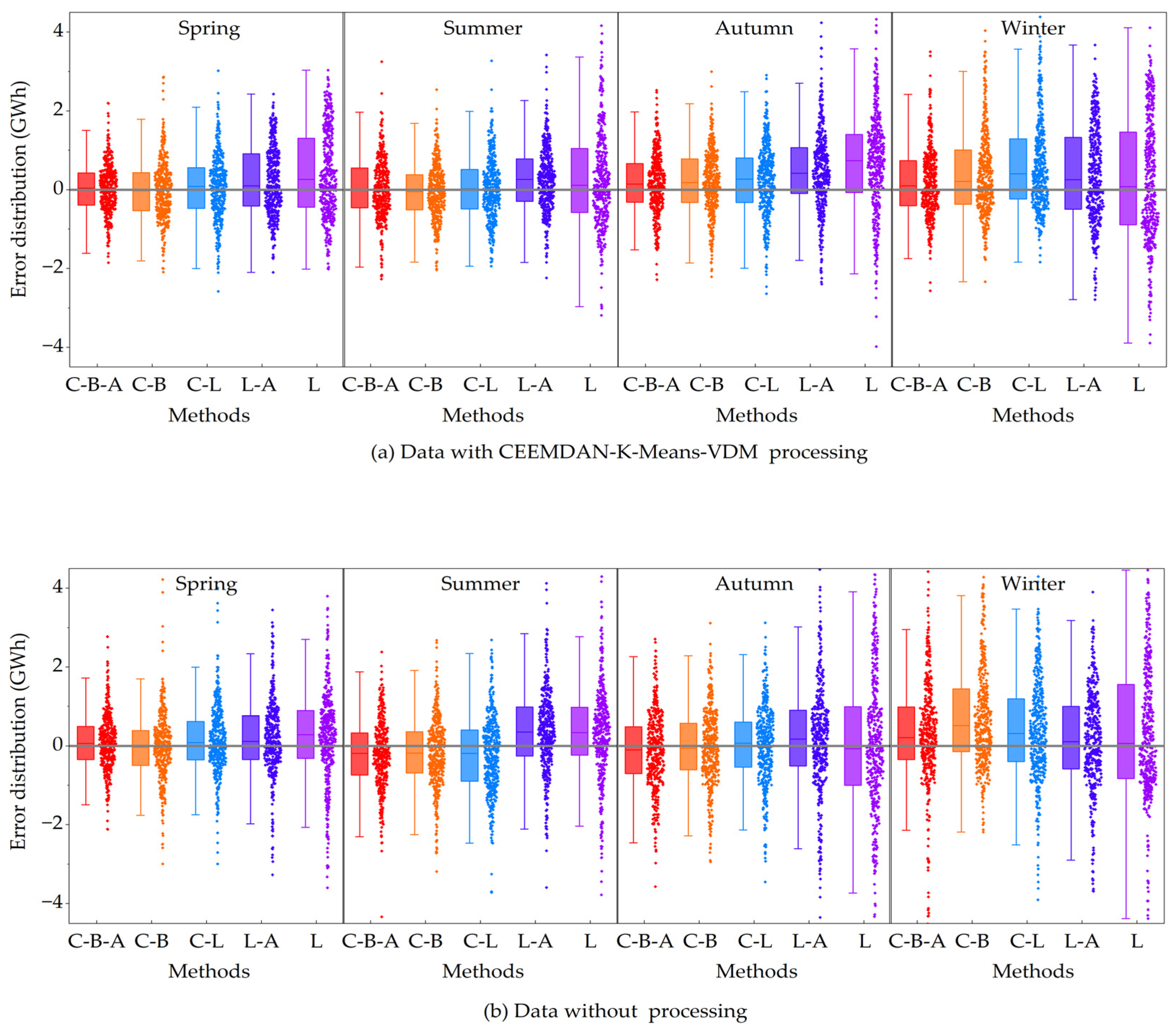
The boxplots and error distributions in Figure 13 show hourly differences between actual and predicted loads across four seasons of C-B-A, C-B, C-L, L-A and LSTM models, where the dots represent prediction errors, the line in the box indicates the median error, the box’s upper and lower edges represent the 75th and 25th percentiles, and the whiskers show the maximum and minimum values, excluding outliers.
Table 9 compares the prediction accuracies of each model using the original data with the CEEMDAN, K-means and VMD processing data. Figure 13a,b, respectively, show the prediction error results obtained by processing the data with CEEMDAN, K-means, VMD and the original data. The following can be found:
  • Overall, except for the L model, the prediction accuracy of all models is improved by using CEEMDAN, K-means, and VMD for data processing. The MSE is improved by up to 1.09 GWh2, and the MAPE is improved by up to 0.45%;
  • Figure 13 shows that performing CEEMDAN, K-means and VMD processing on the original load sequence and using the processed data for prediction can reduce the difference between the actual load and the prediction. Only the median error of some models deviates from the “0” value in autumn and winter. Overall, the median error of each model in the four seasons shows an approach to the “0” value;
  • Compared with Figure 13b, in Figure 13a, except for L-A in spring and winter, and L in spring, summer and winter, most models have a reduced box height across all four seasons. Meanwhile, the error distribution in Figure 13a shows a bell-shaped feature. All these indicate that the modal decomposition and clustering of the original data can further improve the prediction accuracy;
  • Moreover, the processed data are more conducive to the extraction of features by CNN. The errors of C-B-A, C-B and C-L show a more obvious normal distribution;
  • Although the normal characteristics of the error distributions of L-A and LSTM in Figure 13a are relatively less obvious, compared with the situation in Figure 13b, the errors have a significant tendency to concentrate towards the median line, and the outliers decrease.
Overall, processing the original load sequences with CEEMDAN, K-means and VMD and applying them for hourly load prediction can enhance the prediction accuracy of each model. Additionally, the processed sequence data are more conducive to helping CNN better extract historical load sequence information.

4.5. Influence of Training Data Quantity

In addition to the model’s internal structure and the hyper-parameter settings, the prediction accuracy of the model is also affected by the volume and diversity of the training dataset. Complex models, with more parameters to estimate, are hard to train accurately with limited data. When training data are scarce, deep neural networks may overfit by learning the data’s noise and specific patterns instead of general trends. This prevents the models from generalizing to new situations and leads to poor test set performance. In reality, sometimes it is impossible to accurately obtain sufficient raw data for model prediction, which adds to the complexity of making accurate predictions.
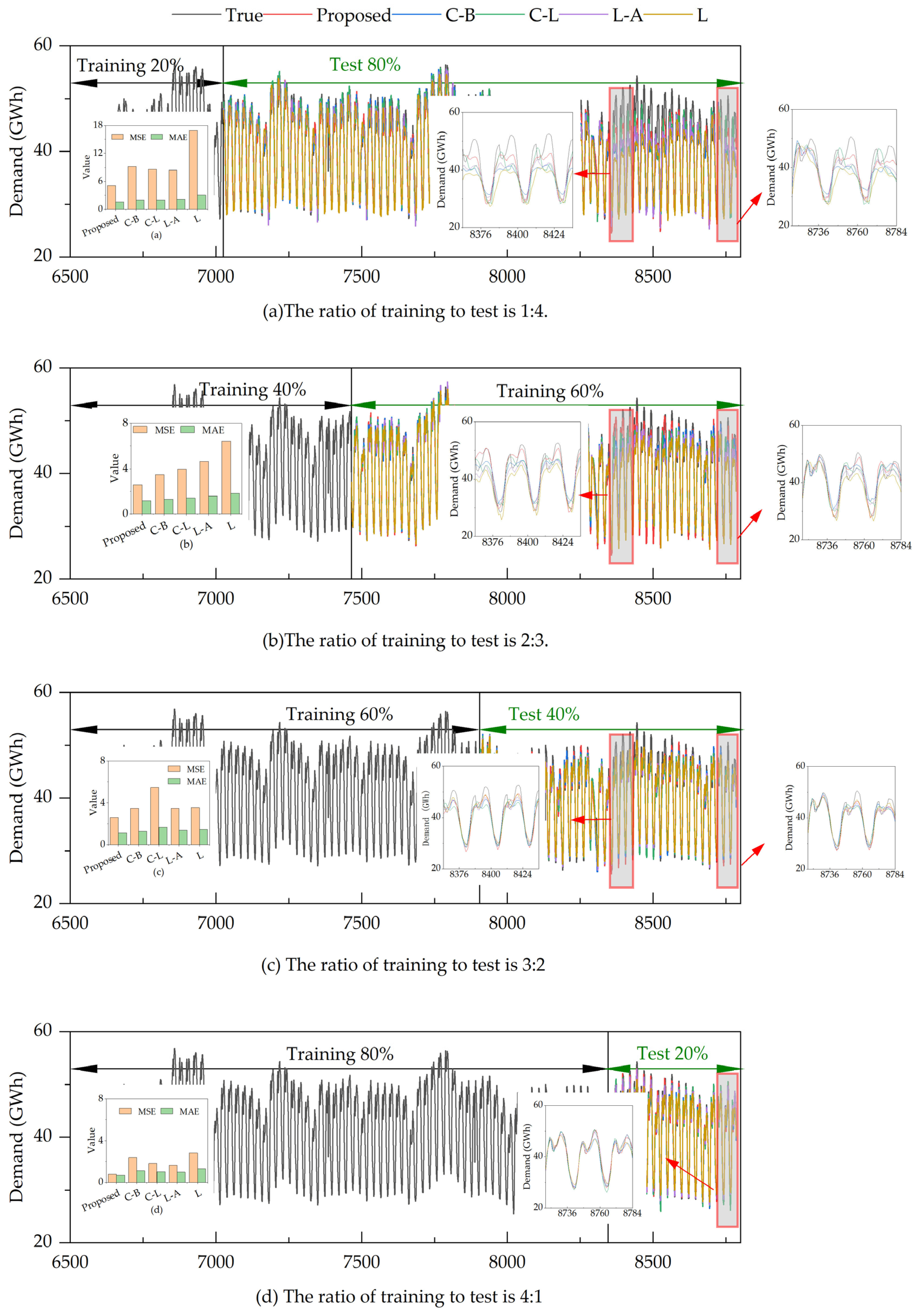
This section examines how training data quantity affects the predictive performance of each model. Winter, where all models show the lowest accuracy, is chosen for this test. The training and test sets are split in ratios of 1:4, 2:3, and 3:2 to explore each model’s training data requirements. Figure 14 presents the hourly comparisons of each model’s predictions with the original data, along with MSE and MAE error indicators, for training set proportions of 20%, 40%, 60% and 80%, respectively. It shows that having sufficient training data is crucial for improving predictive accuracy. A substantial reduction in the training set hinders the model’s ability to learn regular features:
  • When the training set is 20%, the MSE and MAE of the proposed model are 5.04 GWh2 and 1.59 GWh, respectively. The MSE and MAE of C-B, C-L and L-A are approximately 9 GWh2 and 2 GWh, respectively. The MSE of LSTM reaches 16.95 GWh2, and the MAE is 3.07 GWh. By comparing the prediction effects of each model with the actual load between the 8364–8436 period, where all models performed poorly, and the final 8720–8784 period, it is found that C-L and LSTM fail to capture the second daily load peak information—which is the highest power demand peak throughout the day, predicting it to be significantly lower than the first load peak. However, C-L achieves a relatively accurate prediction of the first load peak. While L-A improves the prediction of the highest peak, its estimate was here still lower than that of the first peak. By contrast, the proposed model and C-B show better sequential information extraction, predicting the second peak as the day’s highest. However, all models underpredict the peaks, with the second peak predictions deviating most from the actual value;
  • When the training set is 40%, all models show improved prediction accuracy. The MSE and MAE of the proposed model are 2.58 GWh2 and 1.16 GWh respectively. LSTM remains the least accurate, with an MSE of 6.42 GWh2 and an MAE of 1.80 GWh. Most models, except C-L, have learned to predict two daily load peaks, with the second higher than the first. In the periods 8364–8436 and 8720–8784, the proposed model, followed by C-B, L-A, and LSTM (excluding C-L), shows the smallest deviations in trend and value from the actual load
  • When the training set is 60%, the prediction accuracy of L-A and LSTM improves significantly, with MSE values around 3.50 GWh2 and MAE around 1.40 GWh. However, the prediction accuracy of C-L drops substantially, with an MSE of 5.48 GWh2 and an MAE of 1.66 GWh, and it still fails to capture the second load peak. Despite more training data, the proposed model, C-B, and L-A may have captured noise, leading to a third predicted peak between the two actual peaks. This is also the reason why the changes in the prediction accuracy of the proposed model and C-B after the increase in training data are extremely slight;
  • When the training set is 80%, all models demonstrate the learning of general trends in the training data. The proposed model best fits the load data, showing the smallest differences from actual load levels in terms of both magnitude and duration. C-L and L-A also predict load peaks well, but fail to capture the durations of these peaks and valleys. C-B and LSTM capture some information about the durations of peaks and valleys, but generally underpredict load peaks.

4.6. Model Generalization Test

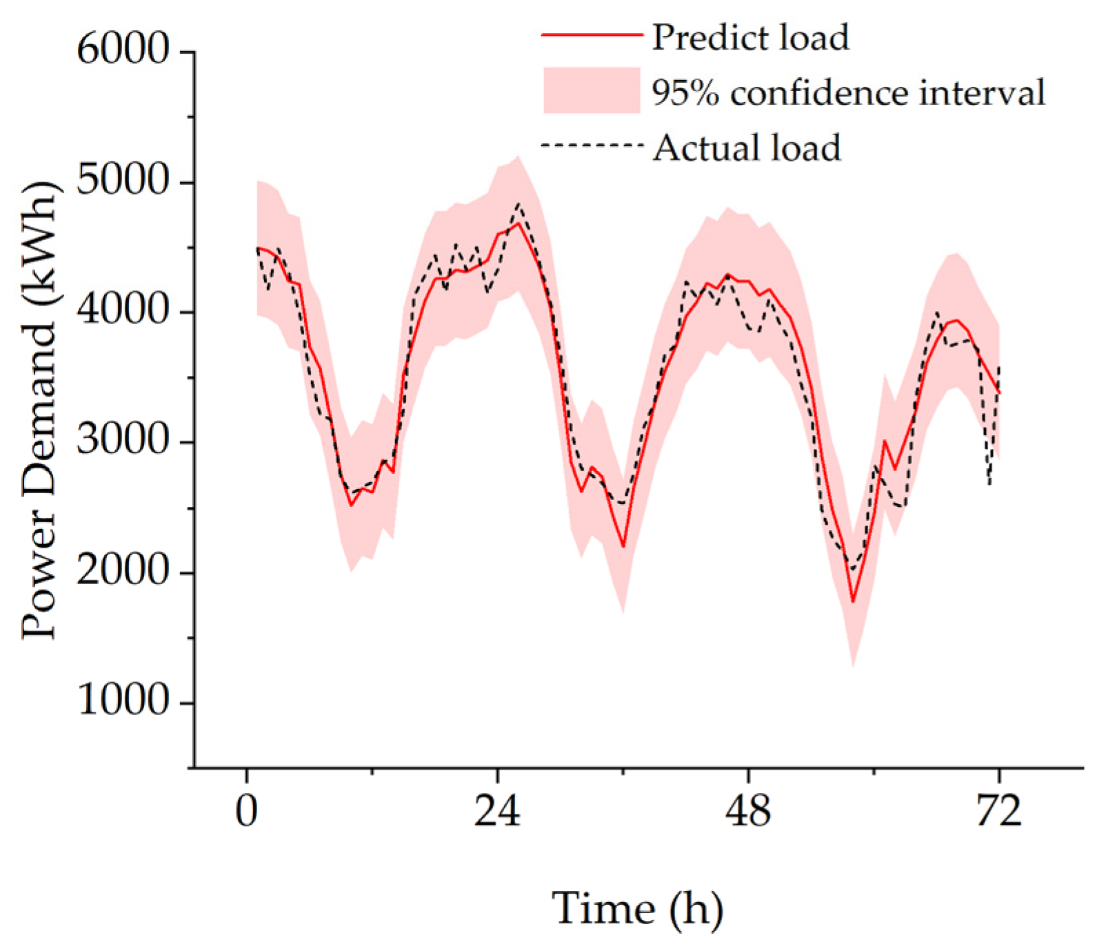
The proposed model is applied to predict the power load of a tourist-oriented island to test its generalization. This area’s load and temperature distribution differs greatly from in the study case. The 1121-samples database is more volatile and uncertain due to the local tourism expansion, and there are a few discontinuous data. The proposed model achieved an SD of 264.34 kWh, a MAPE of 5.6%, and an R2 of 90% on this dataset. As shown in Figure 15, despite inadequate training data, the model performed well in predicting load levels and overall trends. Except for the mutation that occurred at the end, the actual loads all fell within the predicted 95% confidence band. In summary, the proposed model demonstrates a good generalization ability and robustness.

5. Conclusions

This study introduces a data-processing method that uses CEEMDAN, K-means, and VMD sequentially on raw data for feature decomposition and clustering, and to extract the significant regularity of historical data in terms of seasonal, weekly and holiday characteristics, as well as the uncertainty in terms of hourly randomness and diurnal variation characteristics, which is more conducive to the capturing of data characteristics by the model. A CNN-BiLSTM-attention model is proposed for the power load forecasting. The proposed method is compared with other deep learning methods to prove its practicability and superiority.
The CNN and LSTM models capture climate and time information in multivariate time series, forecasting power loads for four seasons. The proposed model outperforms CNN-BiLSTM, CNN-LSTM, LSTMM-attention and LSTM in load prediction across all four seasons. Furthermore, ablation experiments on the model verified that each component contributed to the entire model. Moreover, CEEMDAN, K-means and VMD-processed data here show an enhancing effect on model feature extraction and prediction accuracy. Also, the generalization ability of the model has been verified on a small-batch dataset with strong fluctuations. Finally, through different divisions of the scale of the training data set, the influence of the amount of training data on the prediction accuracy and prediction trend of the model is here analyzed. The results indicate that the proposed model is efficient and stable, outperforming existing benchmarks.
  • The proposed CNN-BiLSTM-attention network, based on CEEMDAN, K-means and VMD data processing, has MAPE values of 1.41%, 1.25%, 1.08% and 1.67% in spring, summer, autumn, and winter, respectively. The annual cross-seasonal SD is 0.77 GWh;
  • The proposed model and contrast models perform best in spring, followed by summer, with the largest prediction errors in winter;
  • Predicting with mode functions from CEEMDAN, K-means and VMD decomposition, as well as clustering, improves model prediction accuracy compared to using raw data;
  • Mode functions help CNN better extract historical load sequence information, with errors showing a more obvious normal distribution;
  • Insufficient training data may hinder the model’s learning of daily peak load features, and cause BiLSTM and attention models to capture noise features;
  • The proposed model best fits load peaks and valleys in terms of magnitude and duration.
As renewable energy’s proportion in power systems continuously increases, long-term load forecasting is crucial for its effective integration and planning. Long-term load forecasting helps anticipate power market risks, determine a reasonable scale and distribution of renewable energy access, and optimize system operations, thus boosting the renewable energy penetration rate and enhancing power system stability. The proposed model forecasts long-term power loads using temperature, one hour in a day, one day in a week, and holiday indicator features. Moreover, power usage patterns and load curve distributions vary across industries and user groups. Economic and climate features (e.g., cooling needs in cold vs. tropical areas) also significantly impact power load demands. The current dataset lacks information on these features. Future work will collect more diverse data and test the model’s generalization in different climate zones or years, so as to explore the computational efficiency and limitations of the model on different volumes datasets.

Author Contributions

Conceptualization, X.L., H.T. and P.W.; methodology, X.L. and J.S.; software, X.L. and J.S.; validation, X.L., J.S. and H.M.; formal analysis, X.L. and H.M.; investigation, J.S. and W.D.; resources, J.S. and W.D.; data curation, J.S. and W.D.; writing—original draft preparation, X.L., J.S., H.M. and W.D.; writing—review and editing, H.T. and P.W.; visualization, X.L. and J.S.; supervision, H.T. and P.W.; project administration, X.L. and P.W.; funding acquisition, X.L. and P.W. All authors have read and agreed to the published version of the manuscript.

Funding

Supported by the Strategic Priority Research Program of Chinese Academy of Sciences, Grant No. XDC0190104.

Data Availability Statement

All data that support the findings of this study are included within this article. Other related data associated with this study can be made available upon request.

Conflicts of Interest

The authors declare no conflicts of interest. The funders had no role in the design of the study; in the collection, analyses, or interpretation of data; in the writing of the manuscript; or in the decision to publish the results.

References

  1. Raza, M.Q.; Khosravi, A. A review on artificial intelligence based load demand forecasting techniques for smart grid and buildings. Renew. Sustain. Energy Rev. 2015, 50, 1352–1372. [Google Scholar] [CrossRef]
  2. Aslam, S.; Herodotou, H.; Mohsin, S.M.; Javaid, N.; Ashraf, N.; Aslam, S. A survey on deep learning methods for power load and renewable energy forecasting in smart microgrids. Renew. Sustain. Energy Rev. 2021, 144, 110992. [Google Scholar] [CrossRef]
  3. Ahmad, T.; Zhang, H.C.; Yan, B. A review on renewable energy and electricity requirement forecasting models for smart grid and buildings. Sustain. Cities Soc. 2020, 55, 102052. [Google Scholar] [CrossRef]
  4. Fumo, N.; Rafe Biswas, M.A. Regression analysis for prediction of residential energy consumption. Renew. Sustain. Energy Rev. 2015, 47, 332–343. [Google Scholar] [CrossRef]
  5. Ostertagova, E.; Ostertag, O. Forecasting Using Simple Exponential Smoothing Method. Acta Electrotech. Inform. 2012, 12, 62–66. [Google Scholar] [CrossRef]
  6. Pan, Z.; Han, X. A multi-dimensional method of nodal load forecasting in power grid. Dianli Xitong Zidonghua/Autom. Electr. Power Syst. 2012, 36, 47–52. [Google Scholar]
  7. Amber, K.P.; Aslam, M.W.; Hussain, S.K. Electricity consumption forecasting models for administration buildings of the UK higher education sector. Energy Build. 2015, 90, 127–136. [Google Scholar] [CrossRef]
  8. Vu, D.H.; Muttaqi, K.M.; Agalgaonkar, A.P. A variance inflation factor and backward elimination based robust regression model for forecasting monthly electricity demand using climatic variables. Appl. Energy 2015, 140, 385–394. [Google Scholar] [CrossRef]
  9. Beiraghi, M.; Ranjbar, A.M. Ieee, Discrete Fourier Transform Based Approach to Forecast Monthly Peak Load. In Proceedings of the 2011 Asia-Pacific Power and Energy Engineering Conference (Appeec), Wuhan, China, 25–28 March 2011. [Google Scholar]
  10. Ai, X.; Zhou, Z.; Wei, Y.; Zhang, H.; Li, L. Bidding Strategy for Time-shiftable Loads Based on Autoregressive Integrated Moving Average Model. Dianli Xitong Zidonghua/Autom. Electr. Power Syst. 2017, 41, 26–31+104. [Google Scholar]
  11. Liu, Y.; Xu, L. High-performance Back Propagation Neural Network Algorithm for Classification of Mass Load Data. Dianli Xitong Zidonghua/Autom. Electr. Power Syst. 2018, 42, 96–103. [Google Scholar]
  12. Su, X.; Liu, T.; Cao, H.; Jiao, H.; Yu, Y.; He, C.; Shen, J. A Multiple Distributed BP Neural Networks Approach for Short-term Load Forecasting Based on Hadoop Framework. Zhongguo Dianji Gongcheng Xuebao/Proc. Chin. Soc. Electr. Eng. 2017, 37, 4966–4973. [Google Scholar]
  13. Wu, X.; He, J.; Zhang, P.; Hu, J. Power system short-term load forecasting based on improved random forest with grey relation projection. Dianli Xitong Zidonghua/Autom. Electr. Power Syst. 2015, 39, 50–55. [Google Scholar]
  14. Wu, Q.; Gao, J.; Hou, G.; Han, B.; Wang, K.; Li, G. Short term load forecasting support vector machine algorithm based on multi-source heterogeneous fusion of load factors. Autom. Electr. Power Syst. 2016, 40, 67–72+92. [Google Scholar]
  15. Kim, T.Y.; Cho, S.B. Predicting residential energy consumption using CNN-LSTM neural networks. Energy 2019, 182, 72–81. [Google Scholar] [CrossRef]
  16. Wan, A.P.; Chang, Q.; Al-Bukhaiti, K.; He, J.B. Short-term power load forecasting for combined heat and power using CNN-LSTM enhanced by attention mechanism. Energy 2023, 282, 128274. [Google Scholar] [CrossRef]
  17. Li, Z.; Wang, Q.; Wang, J.Q.; Qu, H.B.; Dong, J.C.; Dong, Z. ELSTM: An improved long short-term memory network language model for sequence learning. Expert Syst. 2024, 41, e13211. [Google Scholar] [CrossRef]
  18. Sutskever, I.; Vinyals, O.; Le, Q.V. Sequence to sequence learning with neural networks. In Proceedings of the 28th International Conference on Neural Information Processing Systems, Montreal, QC, Canada, 8–13 December 2014; MIT Press: Cambridge, MA, USA, 2014; Volume 2, pp. 3104–3112. [Google Scholar]
  19. Geng, Y.M. Design of English teaching speech recognition system based on LSTM network and feature extraction. Soft Comput. 2023, 28, 13873–13883. [Google Scholar] [CrossRef]
  20. Bouktif, S.; Fiaz, A.; Ouni, A.; Serhani, M.A. Multi-Sequence LSTM-RNN Deep Learning and Metaheuristics for Electric Load Forecasting. Energies 2020, 13, 391. [Google Scholar] [CrossRef]
  21. Bouktif, S.; Fiaz, A.; Ouni, A.; Serhani, M.A. Optimal Deep Learning LSTM Model for Electric Load Forecasting using Feature Selection and Genetic Algorithm: Comparison with Machine Learning Approaches. Energies 2018, 11, 1636. [Google Scholar] [CrossRef]
  22. Kong, W.C.; Dong, Z.Y.; Jia, Y.W.; Hill, D.J.; Xu, Y.; Zhang, Y. Short-Term Residential Load Forecasting Based on LSTM Recurrent Neural Network. IEEE Trans. Smart Grid 2019, 10, 841–851. [Google Scholar] [CrossRef]
  23. Jixiang, L.U.; Qipei, Z.; Zhihong, Y.; Mengfu, T.U.; Jinjun, L.U.; Hui, P. Short-term Load Forecasting Method Based on CNN-LSTM Hybrid Neural Network Model. Autom. Electr. Power Syst. 2019, 43, 131–137. [Google Scholar]
  24. He, Q.Y.; Su, Y.X. Ieee, Residential Load Forecasting Based on CNN-LSTM and Non-uniform Quantization. In Proceedings of the 2022 12th International Conference on Power and Energy Systems, ICPES, Guangzhou, China, 23–25 December 2022; pp. 586–591. [Google Scholar]
  25. Song, J.C.; Zhang, L.Y.; Xue, G.X.; Ma, Y.P.; Gao, S.; Jiang, Q.L. Predicting hourly heating load in a district heating system based on a hybrid CNN-LSTM model. Energy Build. 2021, 243, 110998. [Google Scholar] [CrossRef]
  26. Sekhar, C.; Dahiya, R. Robust framework based on hybrid deep learning approach for short term load forecasting of building electricity demand. Energy 2023, 268, 126660. [Google Scholar] [CrossRef]
  27. Liu, H.; Yue, D.; Miao, G.; Wang, L.; Wang, G.; Zhu, H. Short-Term Load Prediction Technology Based on Attention-CNN-GRU Hybrid Neural Network. Electr. Eng. 2024, 9, 20–23. [Google Scholar]
  28. Du, S.D.; Li, T.R.; Yang, Y.; Horng, S.J. Multivariate time series forecasting via attention-based encoder-decoder framework. Neurocomputing 2020, 388, 269–279. [Google Scholar] [CrossRef]
  29. Ning, Z.; Bowen, S.; Mingming, X.; Lei, P.; Guang, F. Enhancing photovoltaic power prediction using a CNN-LSTM-attention hybrid model with Bayesian hyperparameter optimization. Glob. Energy Interconnect. 2024, 7, 667–681. [Google Scholar]
  30. Somu, N.; Raman, M.R.G.; Ramamritham, K. A deep learning framework for building energy consumption forecast. Renew. Sustain. Energy Rev. 2021, 137, 110591. [Google Scholar] [CrossRef]
  31. Lv, L.L.; Wu, Z.Y.; Zhang, J.H.; Zhang, L.; Tan, Z.Y.; Tian, Z.H. A VMD and LSTM Based Hybrid Model of Load Forecasting for Power Grid Security. IEEE Trans. Ind. Inform. 2022, 18, 6474–6482. [Google Scholar] [CrossRef]
  32. Aksan, F.; Suresh, V.; Janik, P.; Sikorski, T. Load Forecasting for the Laser Metal Processing Industry Using VMD and Hybrid Deep Learning Models. Energies 2023, 16, 5381. [Google Scholar] [CrossRef]
  33. Gao, B.X.; Huang, X.Q.; Shi, J.S.; Tai, Y.H.; Zhang, J. Hourly forecasting of solar irradiance based on CEEMDAN and multi-strategy CNN-LSTM neural networks. Renew. Energy 2020, 162, 1665–1683. [Google Scholar] [CrossRef]
  34. Hong, T.; Fan, S. Probabilistic electric load forecasting: A tutorial review. Int. J. Forecast. 2016, 32, 914–938. [Google Scholar] [CrossRef]
  35. Torres, M.E.; Colominas, M.A.; Schlotthauer, G.; Flandrin, P. A complete ensemble empirical mode decomposition with adaptive noise. In Proceedings of the 2011 IEEE International Conference on Acoustics, Speech and Signal Processing (ICASSP), Prague, Czech Republic, 22–27 May 2011; pp. 4144–4147. [Google Scholar]
  36. UR Rehman, N.; Mandic, D.P. Empirical Mode Decomposition for Trivariate Signals. IEEE Trans. Signal Process. 2010, 58, 1059–1068. [Google Scholar] [CrossRef]
  37. Richman, J.S.; Moorman, J.R. Physiological time-series analysis using approximate entropy and sample entropy. Am. J. Physiol.-Heart Circ. Physiol. 2000, 278, H2039–H2049. [Google Scholar] [CrossRef]
  38. Dragomiretskiy, K.; Zosso, D. Variational Mode Decomposition. IEEE Trans. Signal Process. 2014, 62, 531–544. [Google Scholar] [CrossRef]
  39. Pascanu, R.; Mikolov, T.; Bengio, Y. On the difficulty of training recurrent neural networks. In Proceedings of the 30th International Conference on International Conference on Machine Learning, Atlanta, GA, USA, 16–21 June 2013; Volume 28, pp. III-1310–III-1318. [Google Scholar]
  40. Ahmad, M.W.; Mourshed, M.; Rezgui, Y. Trees vs Neurons: Comparison between random forest and ANN for high-resolution prediction of building energy consumption. Energy Build. 2017, 147, 77–89. [Google Scholar] [CrossRef]
  41. Ahmad, A.S.; Hassan, M.Y.; Abdullah, M.P.; Rahman, H.A.; Hussin, F.; Abdullah, H.; Saidur, R. A review on applications of ANN and SVM for building electrical energy consumption forecasting. Renew. Sustain. Energy Rev. 2014, 33, 102–109. [Google Scholar] [CrossRef]
  42. Mat Daut, M.A.; Hassan, M.Y.; Abdullah, H.; Rahman, H.A.; Abdullah, M.P.; Hussin, F. Building electrical energy consumption forecasting analysis using conventional and artificial intelligence methods: A review. Renew. Sustain. Energy Rev. 2017, 70, 1108–1118. [Google Scholar] [CrossRef]
  43. Yao, C.; Yang, P.; Liu, Z. Load Forecasting Method Based on CNN-GRU Hybrid Neural Network. Power Syst. Technol. 2020, 44, 3416–3424. [Google Scholar]
  44. Hochreiter, S.; Schmidhuber, J. Long Short-Term Memory. Neural Comput. 1997, 9, 1735–1780. [Google Scholar] [CrossRef]
  45. Gers, F.A.; Schmidhuber, J.; Cummins, F. Learning to forget: Continual prediction with LSTM. Neural Comput. 2000, 12, 2451–2471. [Google Scholar] [CrossRef]
  46. Ghimire, S.; Deo, R.C.; Raj, N.; Mi, J. Deep solar radiation forecasting with convolutional neural network and long short-term memory network algorithms. Appl. Energy 2019, 253, 113541. [Google Scholar] [CrossRef]
  47. Chen, Y.; Zhang, S.; Zhang, W.; Peng, J.; Cai, Y. Multifactor spatio-temporal correlation model based on a combination of convolutional neural network and long short-term memory neural network for wind speed forecasting. Energy Convers. Manag. 2019, 185, 783–799. [Google Scholar] [CrossRef]
  48. Graves, A.; Schmidhuber, J. Framewise phoneme classification with bidirectional LSTM and other neural network architectures. Neural Netw. 2005, 18, 602–610. [Google Scholar] [CrossRef] [PubMed]
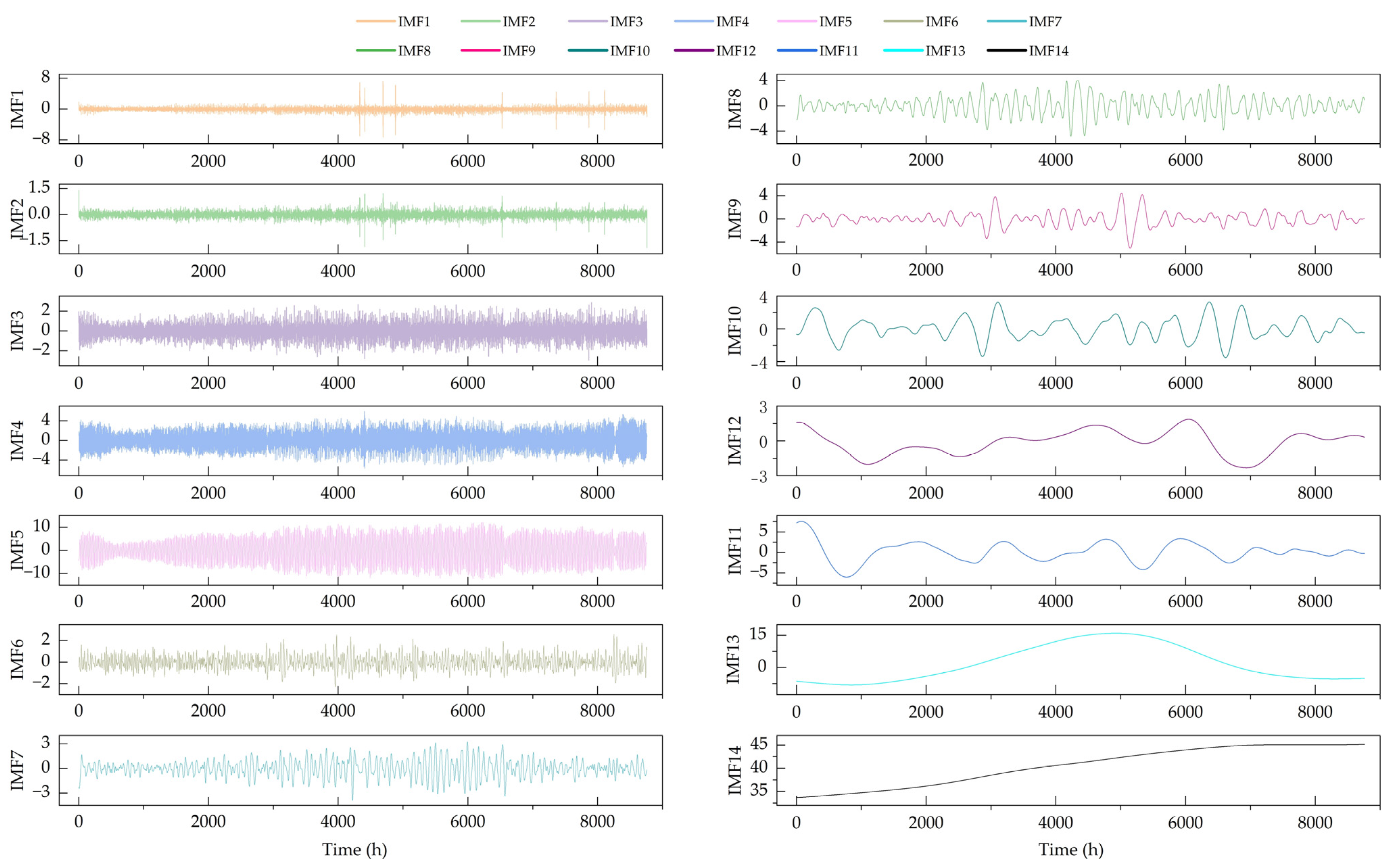
Figure 1. The IMFs of the CEEMDAN method (GWh).
Energies 18 02675 g001
Figure 2. The Silhouette Coefficient, SSE and clustering result: (a) the Silhouette Coefficient of different K values; (b) the SSE of different K values; (c) clustering result when K = 3.
Energies 18 02675 g002
Figure 3. The clusters of the K-means method (GWh).
Energies 18 02675 g003
Figure 4. The power load sequence and IMFs of the VMD method (GWh).
Energies 18 02675 g004
Figure 5. The CNN structure diagram.
Energies 18 02675 g005
Figure 6. The LSTM structure diagram.
Energies 18 02675 g006
Figure 7. The BiLSTM structure diagram.
Energies 18 02675 g007
Figure 8. The attention mechanism structure: c . for optimized context vector; a for attention weight; h for hidden layer; x for input.
Energies 18 02675 g008
Figure 9. The structure of the proposed model: Y represents for “Yes”; N represents for “No”.
Energies 18 02675 g009
Figure 10. Model MSE change (GWh2).
Energies 18 02675 g010
Figure 11. Comparison of predicted load and actual load.
Energies 18 02675 g011
Figure 12. Prediction results using the proposed model and benchmark models. The units of MSE, RMSE and MAPE are GWh2, GWh, and GWh respectively.
Energies 18 02675 g012
Figure 13. Error box plots and distributions of each model: (a) data with CEEMDAN, K-means, VMD processing; (b) data without processing.
Energies 18 02675 g013
Figure 14. Comparison of prediction results obtained by different split ratios of training data and test data. (a) The ratio of training to test is 1:4. (b) The ratio of training to test is 2:3. (c) The ratio of training to test is 3:2. (d) The ratio of training to test is 4:1.
Energies 18 02675 g014
Figure 15. Generalization test prediction results.
Energies 18 02675 g015
Table 1. The sample entropy values of 14 IMFs.
IMFSample EntropyIMFSample Entropy
11.593380.1343
21.879190.0618
31.8332100.0311
40.7258110.0121
50.5189120.0041
60.5795130.0017
70.2996140.0002
Table 2. CNN-BiLSTM-attention architecture parameters.
LayersLayer ParametersActivation FunctionsInitializers
Sequence input layerNumber of features5--
CNN2DKernel size[1, 3]State activation function-ReluWeights Initializer-Glorot
Bias Initializer-zeros
Filter16--
Stride1--
PaddingSame--
Pooling LayerPool Size[1, 2]Pooling function-Max Pooling-
Stride2--
PaddingSame--
BiLSTM LayerNumber of hidden layers20State Activation Function-tanhInput weight initializer-Glorot
Recurrent weight
Initializer-orthogonal
Bias Initializer-unit
forget gate
Attention LayerNum of Heads2-Weights Initializer-Glorot
Bias Initializer-zeros
Num of Key Channels2--
Attention mechanismSoftmax--
Dropout LayerProbability0.1--
Fully Connected LayerOutput Size1--
Table 3. Hyper-parameter setting of CNN-BiLSTM-attention.
ParameterSetting
OptimizerAdam
Execution EnvironmentCPU
Loss FunctionMean Squared Error (MSE)
Max Epoch150
Gradient Threshold1
L2 Regularization0.0001
Learning rate0.001
Table 4. Error change process.
SeasonMethodEpoch
11020304050
SpringProposed0.690.110.060.060.050.05
C-B0.520.060.040.050.040.04
C-L0.510.080.050.060.050.05
L-A0.400.140.100.080.070.07
L0.830.160.120.110.100.08
SummerProposed0.700.100.070.060.050.05
C-B0.770.070.050.060.040.04
C-L0.590.100.090.090.080.08
L-A0.630.140.110.090.090.07
L0.520.130.100.090.090.08
AutumnProposed0.400.080.060.050.050.04
C-B0.650.070.060.050.050.05
C-L0.580.100.080.070.060.07
L-A0.690.160.140.100.080.08
L0.650.140.120.110.100.09
WinterProposed0.600.090.060.060.050.04
C-B0.360.060.050.050.060.04
C-L0.650.100.080.070.070.06
L-A0.520.150.100.090.080.08
L0.610.170.130.120.110.09
Table 5. Model training time for four seasons (seconds).
SeasonProposed
(5 Database)
C-BC-LL-AL
Spring821515107
Summer15316161116
Autumn1343831119
Winter801617810
Total44985794042
Table 6. MSE, RMSE, MAE and R2 forecasted for different models in four seasons.
SeasonMethodEvaluation IndexImprovement
MSERMSEMAEMAPER2MSERMSEMAEMAPER2
GWh2GWhGWh%%GWh2GWhGWh%%
SpringProposed0.390.620.491.4199.10-----
C-B0.710.840.611.8298.350.320.220.120.420.74
C-L0.750.870.641.9298.250.360.240.150.510.84
L-A1.051.020.752.2997.560.660.400.260.881.54
L1.501.230.932.8196.501.120.600.441.402.60
SummerProposed0.570.750.601.2599.13-----
C-B0.820.910.701.4798.740.250.150.100.220.39
C-L1.031.010.801.6698.430.460.260.200.400.71
L-A1.261.120.871.8898.070.690.370.270.631.06
L1.551.240.942.0497.630.980.490.340.791.50
AutumnProposed0.620.790.611.0899.28-----
C-B0.950.970.741.3198.890.330.190.130.230.38
C-L0.990.990.761.3598.840.370.210.150.270.43
L-A1.971.401.031.8897.701.350.620.420.801.57
L3.151.771.352.4296.322.530.990.741.342.96
WinterProposed0.790.890.681.6798.56-----
C-B2.371.541.112.1495.761.570.650.431.192.80
C-L1.791.341.032.4096.761.000.450.350.861.80
L-A1.631.280.992.6397.050.830.380.310.781.51
L2.911.681.313.2994.922.120.780.631.623.64
Table 7. Comparison of the annual forecasting results of different models.
MethodMESDMSERMSEMAEMAPE
GWhGWhGWh2GWhGWh%
Proposed0.110.770.600.770.601.38
C-B−0.021.071.141.070.811.86
C-L−0.081.071.141.070.811.84
L-A−0.211.201.481.220.912.00
L−0.241.482.261.501.142.51
Table 8. The results of Ablation Study.
MethodMESDMSERMSEMAEMAPE
GWhGWhGWh2GWhGWh%
Full Model0.110.770.600.770.601.38%
w/o VDM−0.150.800.670.820.631.46%
w/o CEEMDAN-K-Means-VDM0.011.021.051.020.741.66%
w/o CNN−0.261.091.261.120.871.95%
w/o BiLSTM−0.210.850.770.880.681.58%
w/o Attention0.140.870.780.880.661.54%
Full Model0.110.770.600.770.601.38%
Table 9. Comparison of the forecasting results with and without CEEMDAN, K-means and VMD processing.
SeasonMethodWith ProcessingWithout Processing
MSERMSEMAEMAPER2MSERMSEMAEMAPER2
GWh2GWhGWh%%GWh2GWhGWh%%
SpringProposed0.390.620.491.4199.100.520.720.551.6598.79
C-B0.560.750.581.6798.690.710.840.611.8298.35
C-L0.680.830.651.8998.410.750.870.641.9298.25
L-A0.790.890.722.1698.161.051.020.752.2997.56
L1.361.170.932.8696.841.501.230.932.8196.50
SummerProposed0.570.750.601.2599.130.800.890.691.4598.78
C-B0.500.710.551.1699.240.820.910.701.4798.74
C-L0.630.790.621.3199.041.031.010.801.6698.43
L-A0.720.850.661.4398.901.261.120.871.8898.07
L1.601.270.952.0597.541.551.240.942.0497.63
AutumnProposed0.620.790.611.0899.280.970.980.761.3598.87
C-B0.690.830.651.1599.190.950.970.741.3198.89
C-L0.860.930.731.2899.000.990.990.761.3598.84
L-A1.311.140.881.5798.471.971.401.031.8897.70
L2.131.461.172.0897.523.151.771.352.4296.32
WinterProposed0.790.890.681.6798.561.891.370.982.4896.59
C-B1.341.590.862.1497.582.371.541.112.8595.76
C-L1.731.310.972.4096.901.791.341.032.5296.76
L-A1.671.291.042.6396.991.631.280.992.4597.05
L2.541.591.323.2995.412.911.681.313.2994.92
Disclaimer/Publisher’s Note: The statements, opinions and data contained in all publications are solely those of the individual author(s) and contributor(s) and not of MDPI and/or the editor(s). MDPI and/or the editor(s) disclaim responsibility for any injury to people or property resulting from any ideas, methods, instructions or products referred to in the content.