Green’s Function Approach for Simulating District Heating Networks

Abstract

In this paper, we introduce a mathematical framework for analyzing and optimizing district heating networks by leveraging the Green’s function method. Traditional numerical methods for simulating district heating networks often face computational challenges and lack transparency in revealing cause-and-effect relationships in heat propagation. By treating temperature as a scalar field, we employ Green’s function methods to derive analytical solutions that provide a more transparent and intuitive understanding of how heat propagates through the network in response to various inputs. We demonstrate the application of this framework through two numerical examples involving heating networks. Comparative results show that, under identical hardware conditions, the Green’s function method requires only about one-fifth of the computational time compared to the finite element method for the same case. This approach offers distinct advantages in terms of computational efficiency, accuracy, and interpretability, enabling more effective design, optimization, and control of sustainable district heating systems.

1. Introduction

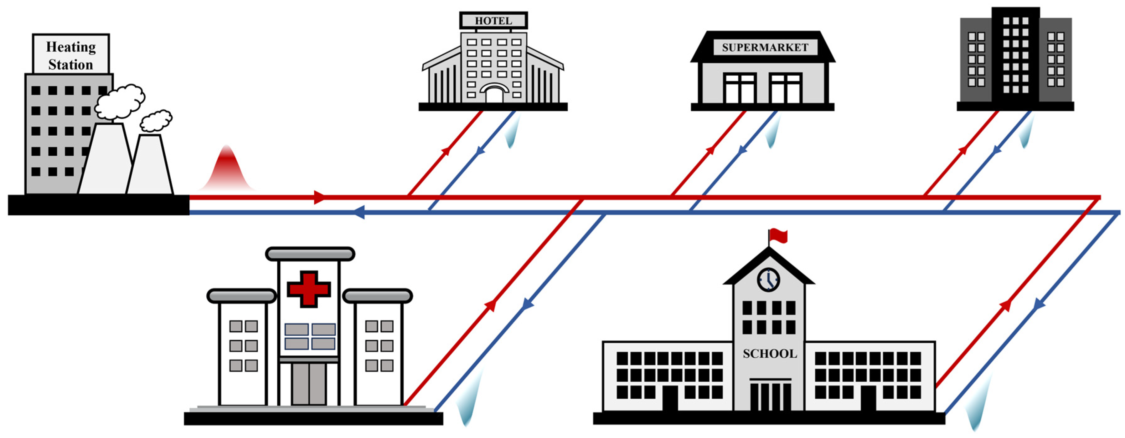
The escalating threat of global warming imposes a strict limit on our carbon budget [1,2]. Reaching net zero CO₂ emissions demands that we be more conscientious than ever about our power generation and consumption and has given rise to smart, integrated energy systems. Across the globe, space heating and cooling consume more than half of our household energy usage [3,4,5]. Among these systems, district heating (Figure 1), which distributes heat from a central heat source to consumers through a system of pipes, is a widely adopted approach. But it remains heavily reliant on fossil fuels like coal and natural gas. In China, for instance, a staggering 90% of district heating energy comes from burning fossil fuels [6]. Diversifying the energy sources that feed district heating systems can make a significant contribution to reducing our global carbon footprint [7]. Optimizing the efficiency of district heating networks offers a double benefit in lowering greenhouse gas emissions. It does so by conserving energy and expanding our ability to integrate clean energy sources into these networks [8,9,10].

A crucial step towards achieving optimized heating efficiency is to model and simulate the temperature profile of heating networks accurately and in a timely manner. Previous works on this subject include a variety of numerical methods, such as finite element [11], plug flow [12,13], steady-state [14,15], dynamic [16,17], and the characteristics method [18,19]. However, a common drawback of these numerical methods—and of solving differential equations in general—is their sensitivity to details of the method itself, the size of the steps taken, and even minute changes in local conditions. For example, when a small dip in one power supply’s output results in a dramatic shift in the stability of the network’s temperature solution, one needs to discern a real chaotic regime from a numerical artifact. To make this task more challenging, these numerical methods often lack transparency when it comes to showing cause and effect across different parts of the system. To see how a user’s heater affects the temperature experienced by other users, one would need to rewrite the entire network’s conditions and solve the problem all over again. Intuitively, however, we should be able to predict this effect simply by knowing the flow through the pipes and the baseline temperature profile, assuming all else stays the same. Furthermore, when multiple users adjust their heaters at different times, we would expect the combined effect to be integrated in a way that aligns with the timestamps of the events.

Central to field theory in physics, Green’s function offers an elegant and effective way to solve partial differential equations. In describing the concept of a field, it is most famously used to solve equations in electrodynamics [20]. In modern physics, Green’s functions have also proven to be a powerful tool for understanding electronic systems, including many-body systems like superconductors [21].

A key advantage of Green’s functions is that they present solutions in a causal form. When using Green’s function methods to solve a partial differential equation, we first solve the homogeneous equation, which describes a uniform spacetime with no source or drain of the field. Then we solve the inhomogeneous equation with an impulse source, hence determining the Green’s function. Once the Green’s function is obtained, the full solution to the differential equation is obtained by integrating over all sources and sinks of the field. In real-world problems, this approach not only provides a clear picture of the causal relationships between the source and the field but also reduces computational complexity.

Green’s functions offer an intuitive framework for visualizing how heating impulses propagate through a network over time, as depicted in Figure 1, making them particularly well-suited for solving heat conduction problems [22,23,24,25]. The limited application of Green’s functions to district heating network analysis may stem from the conceptual challenge of treating temperature as a field. Fundamentally, temperature is a statistical property of an ensemble of excitations rather than a conventional field or excitation in itself. However, the differential equation it obeys in the context of heat propagation and diffusion aligns with that of a scalar field, with heat sources and drains acting as its charges. In a district heating system, the dynamic changes in temperature at each point in the network are controlled by the inputs from heaters and users. By viewing temperature as a scalar field, we can gain valuable insights into how it responds to various triggers. Furthermore, since the differential equation governing temperature is linear, individual solutions can be linearly superimposed. As a result, the final temperature distribution is obtained by integrating the contributions from all inputs across the network [22].

In this paper, we introduce a novel framework for solving district network heating problems by leveraging the power of Green’s functions. We begin by investigating the heat conduction equation within a flowing medium subject to heat dissipation. We derive solutions for both homogeneous and inhomogeneous cases, incorporating boundary conditions that reflect the network topology. These analytical solutions serve as building blocks for modeling integrated heating networks. To demonstrate the effectiveness of this approach, we apply it to two model systems. By employing the Green’s function method for district heating network computations, we achieve both accurate and computationally efficient solutions for the system’s temperature distribution. Through reasonable approximations, we can derive analytical solutions for even highly complex problems, providing deeper insights into heating system dynamics while streamlining the modeling process.

The remainder of the paper is organized as follows. In Section 2, we introduce the Green’s function method and present analytical Green’s functions of the heat conduction equation under different boundary conditions. In Section 3, we present two numerical examples, illustrating temperature distribution calculations using the Green’s function method, along with a comparison to the finite element method in terms of both accuracy and computational efficiency.

By promoting a new perspective that treats temperature as a field, this work sheds light on how concepts from field theory can enhance the simulation and optimization of complex energy networks. As such, this approach not only equips the energy community with a novel computational method but also introduces a powerful conceptual tool, paving the way for further advancements in the field of integrated energy systems.

2. Green’s Function of the Heat Conduction Equation

2.1. Introduction to the Green’s Function Method

The Green’s function method constitutes a rigorous mathematical framework for solving inhomogeneous partial differential equations (PDEs). This approach enables the construction of complete solutions through the superposition of responses to impulsive excitations. Mathematically, the Green’s function $G(x,t;\xi ,\tau )$ is the solution to a PDE driven by Dirac delta source terms such as $\delta \left(x-\xi \right)\delta (t-\tau )$. Physically, it is the response of the system at point $x$ and time $t$ induced by a unit impulse applied at position $\xi$ and instant $\tau$.

For instance, for the heat conduction equation for water in a one-dimensional pipe:

$$\rho c{\displaystyle \frac{\partial T}{\partial t}}-\kappa {\displaystyle \frac{{\partial }^{2}T}{\partial x^2}}=Q,$$

(1)

the Green’s function $G(x,t;\xi ,\tau )$ is defined as the solution to the equation

$$\rho c{\displaystyle \frac{\partial G}{\partial t}}-\kappa {\displaystyle \frac{{\partial }^{2}G}{\partial x^2}}=\delta \left(x-\xi \right)\delta \left(t-\tau \right)$$

(2)

under specific boundary conditions. Here $T$, $v$, $\rho$, $c$, and $\kappa$ denote the temperature, flow velocity, density, specific heat capacity, and thermal conductivity of water, respectively, while $Q(x,t)$ represents the heat source power per unit volume. The Dirac delta functions $\delta \left(x-\xi \right)$ and $\delta (t-\tau )$ at the right-hand side describe an instantaneous point source located at position $\xi$ and time $\tau$.

Once the Green’s function $G\left(x,t;\xi ,\tau \right)$ of the equation is obtained, the solution to the original PDE under an arbitrary heat source $Q$ can be constructed through integrals. With the initial temperature distribution $T\left(x,0\right)$ and heat source $Q$, the solution to Equation (1) is expressed as:

$$T\left(x,t\right)={\int }_{-\infty }^{\infty }G\left(x,t;\xi ,0\right)T\left(\xi ,0\right)\mathrm{d}\xi +{\int }_0^t{\int }_{-\infty }^{\infty }G\left(x,t;\xi ,\tau \right)Q\left(\xi ,\tau \right)\mathrm{d}\xi \mathrm{d}\tau .$$

(3)

Here, the first integral term describes how the initial temperature distribution evolves over time, while the second double integral term reflects contributions from the heat source $Q(x,t)$. This formulation elegantly separates the effects of the initial state and the external heat source, providing a clear and systematic framework for analyzing the system’s temperature evolution.

2.2. Heat Conduction Equation for a 1D Cylindrical Pipe with a Steady Flow Velocity

Depicting the dynamics of a district heating system requires consideration of both fluid motion and heat transfer processes. However, Equation (1) does not account for the effects of water flow within the pipeline and, therefore, is inadequate.

During the heating process, the average velocity $v$ of the water flow is generally maintained constant. Under this steady-flow condition, the heat conduction equation for a one-dimensional (1D) pipeline can be obtained by considering energy conservation [8]:

$$\rho c{\displaystyle \frac{\partial T(x,t)}{\partial t}}+\rho cv{\displaystyle \frac{\partial T(x,t)}{\partial x}}-\kappa {\displaystyle \frac{{\partial }^{2}T\left(x,t\right)}{\partial x^2}}=Q\left(x,t\right).$$

(4)

On the left-hand side of Equation (4), the time-derivative term, $\rho c{\displaystyle \frac{\partial T(x,t)}{\partial t}}$, describes the rate of change of the internal energy density over time. The spatial-derivative term, $\rho cv{\displaystyle \frac{\partial T(x,t)}{\partial x}}$, accounts for the advection of internal energy density due to the water flow. The third term, $-\kappa {\displaystyle \frac{{\partial }^{2}T\left(x,t\right)}{\partial x^2}}$, is the heat diffusion term, representing heat conduction driven by the temperature gradient.

The heat source term $Q(x,t)$ on the right-hand side of Equation (1) describes the energy exchange between the water and the environment. It consists of three components: a positive term $Q_1$, representing external heating, such as heating from electric boilers; a negative term $Q_2$, corresponding to the heat load from users; and a dissipation term $Q_3=-\mu \left(T-T_0\right)/A$, describing heat loss from the water to the environment. Here, $\mu$ is the heat dissipation coefficient of the pipeline, $T_0$ is the environmental temperature, and $A$ is the cross-sectional area of the pipeline. The dissipation term $Q_3$ is a linear function of temperature. Since $Q_3$ is not a controllable parameter during the heating process, it is convenient to move it to the left-hand side of the equation and no longer treat it as a source term, i.e., letting $Q=Q_1+Q_2$. This yields the modified heat conduction equation:

$$\rho c{\displaystyle \frac{\partial T}{\partial t}}+\rho cv{\displaystyle \frac{\partial T}{\partial x}}-\kappa {\displaystyle \frac{{\partial }^{2}T}{\partial x^2}}+{\displaystyle \frac{\mu \left(T-T_0\right)}{A}}=Q=Q_1+Q_2.$$

(5)

Traditional dynamic simulation approaches typically solve Equation (5) using numerical methods, which often suffer from high computational complexity and cost, and are thus cumbersome for practical use. To address these limitations, in this work, we employ the Green’s function method to solve Equation (5).

However, the complexity of Equation (5) poses significant challenges for directly deriving its Green’s function. Given that the Green’s function for Equation (1) has known analytical solutions under various common boundary conditions, we first apply a mathematical transformation to recast it into a form analogous to Equation (1). This transformation simplifies the problem and allows us to address the additional terms in Equation (5), such as the advection and dissipation terms, using the well-established analytical framework for Equation (1).

To achieve this, we introduce a new function $W(x,t)$ to replace the temperature distribution $T(x,t)$. The function $W(x,t)$ is defined by the relationship

$$W\left(x,t\right)e^{\theta (x,t)}=T\left(x,t\right)-T_0,$$

(6)

where

$$\theta \left(x,t\right)={\displaystyle \frac{v}{2\alpha }}x-\left({\displaystyle \frac{v^2}{4\alpha }}+{\displaystyle \frac{\mu }{A\rho c}}\right)t,$$

(7)

and

$$\alpha ={\displaystyle \frac{\kappa }{\rho c}}.$$

(8)

Substituting Equations (6)–(8) into Equation (2) gives the governing equation for $W(x,t)$:

$$\rho c{\displaystyle \frac{\partial W(x,t)}{\partial t}}-\kappa {\displaystyle \frac{{\partial }^{2}W\left(x,t\right)}{\partial x^2}}=Q\exp \left(-{\displaystyle \frac{vx}{2\alpha }}+{\displaystyle \frac{v^{2}t}{4\alpha }}+{\displaystyle \frac{\mu t}{A\rho c}}\right).$$

(9)

The mathematical transformation above involves two key mappings: the temperature distribution $T(x,t)$ is mapped to $W(x,t)$, and the heat source term $Q$ is mapped to $Q\exp \left(-{\displaystyle \frac{vx}{2\alpha }}+{\displaystyle \frac{v^{2}t}{4\alpha }}+{\displaystyle \frac{\mu t}{A\rho c}}\right)$.

Equations (1) and (9) have identical mathematical forms, so their Green’s functions are also the same, which enables the calculation of $W(x,t)$ using the Green’s function method and subsequently recovers the original temperature distribution $T(x,t)$ using Equation (6). This approach not only simplifies the computational process but also provides a more intuitive framework for understanding the temperature dynamics in the system.

2.3. Green’s Function of Heat Conduction Equation Under Different Boundary Conditions

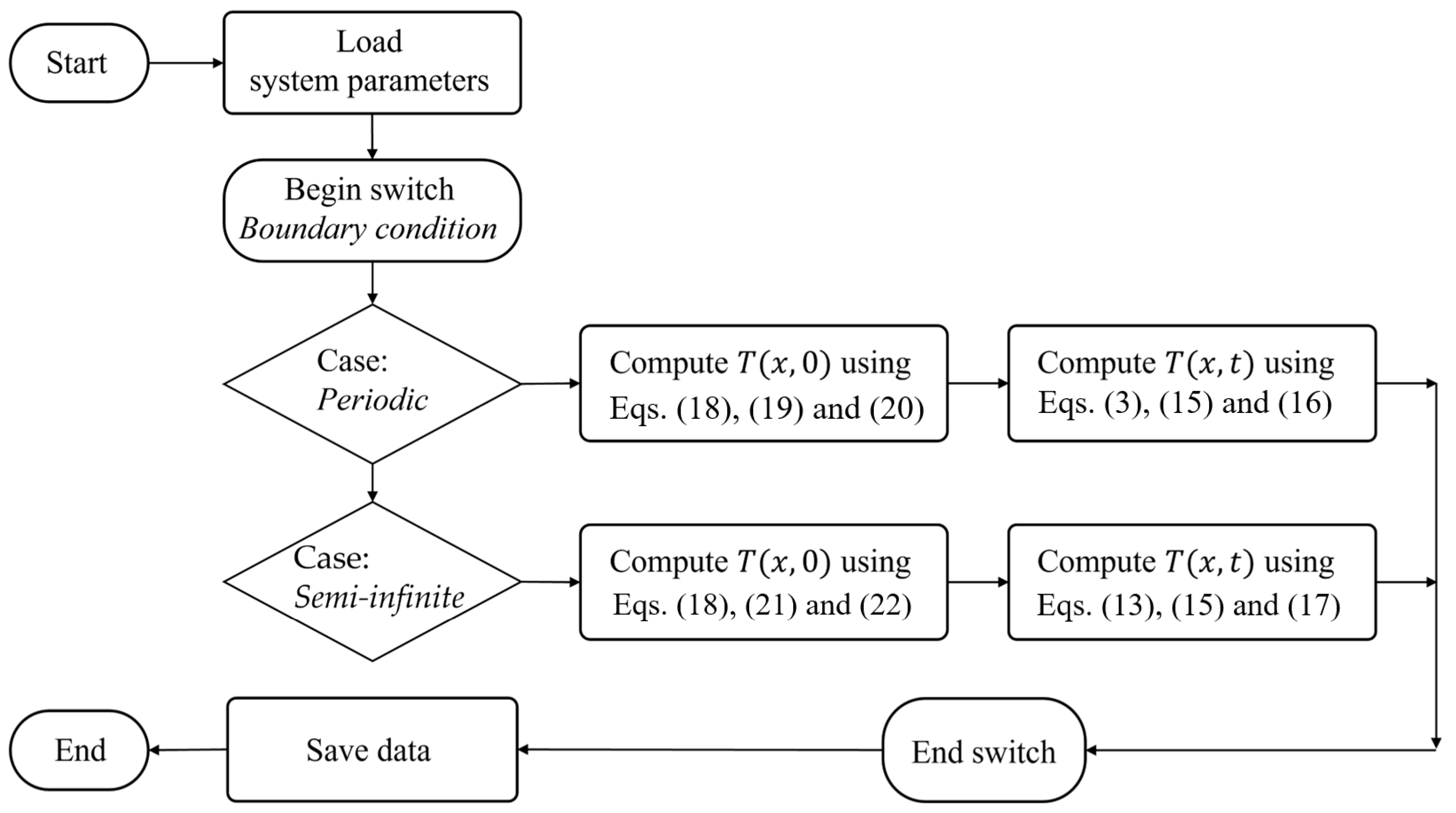
To solve heating problems using the Green’s function method, the first step is to determine the Green’s function of the heat conduction equation (Equations (1) and (9)) under specified boundary conditions.

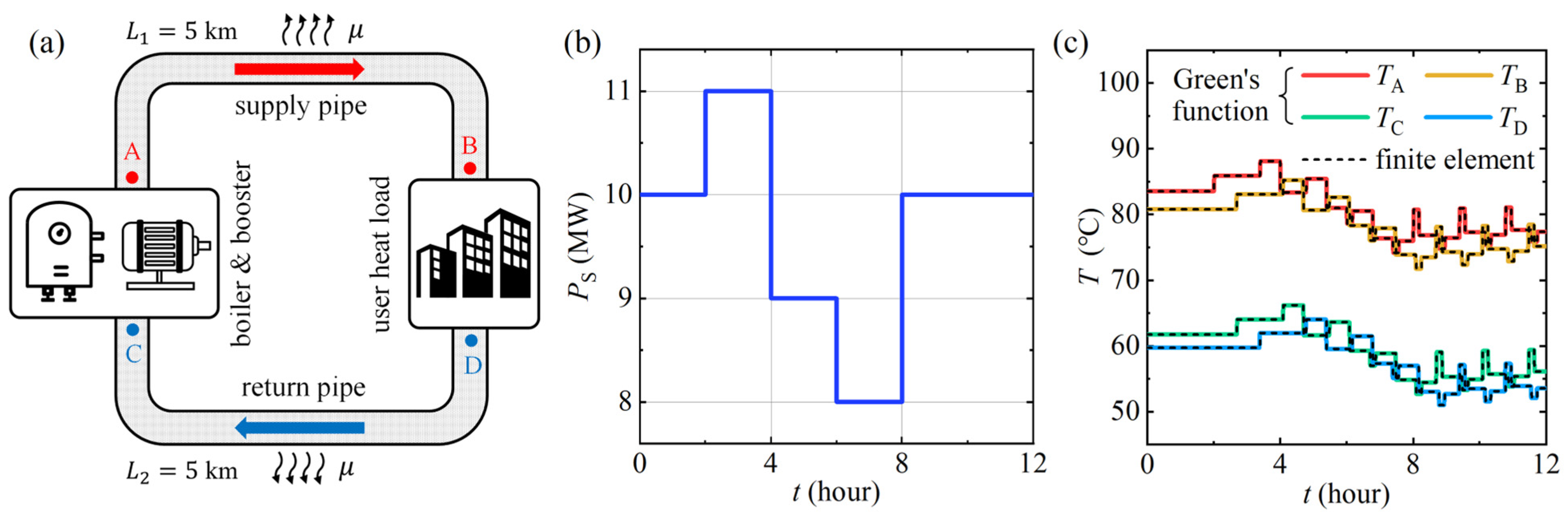
In practical applications, two primary boundary conditions are typically considered: periodic boundary conditions and fixed endpoint temperature boundary conditions for semi-infinite pipes. The periodic boundary condition is employed to model closed-loop heating systems with prescribed external heat sources, as demonstrated in the example in Section 3.1. Meanwhile, the fixed endpoint temperature boundary condition is utilized to model heating pipelines with a controlled inlet temperature, as illustrated in the example in Section 3.2.

2.3.1. Periodic Boundary Condition

The periodic boundary condition is particularly suited for modeling closed-loop pipeline systems. For a pipeline of total length $L$, the periodic condition enforces $T\left(0\right)=T\left(L\right)$ and ${\displaystyle \frac{\mathrm{d}T}{\mathrm{d}x}}\left(0\right)={\displaystyle \frac{\mathrm{d}T}{\mathrm{d}x}}(L)$ at the connection point. These constraints result in a periodic Green’s function with the same period $L$, reflecting the physical reality that thermal disturbances propagate cyclically through the closed-loop pipeline.

For the conventional heat conduction equations like Equations (1) and (9), the Green’s function under periodic boundary conditions admits an analytical solution, expressed as

$$G\left(x,t;\xi ,\tau \right)=\sum _{n\in \mathbb{Z}}{\displaystyle \frac{1}{\sqrt{4\pi \alpha \left(t-\tau \right)}}}\exp \left(-{\displaystyle \frac{{\left(x-\xi -nL\right)}^2}{4\alpha \left(t-\tau \right)}}\right).$$

(10)

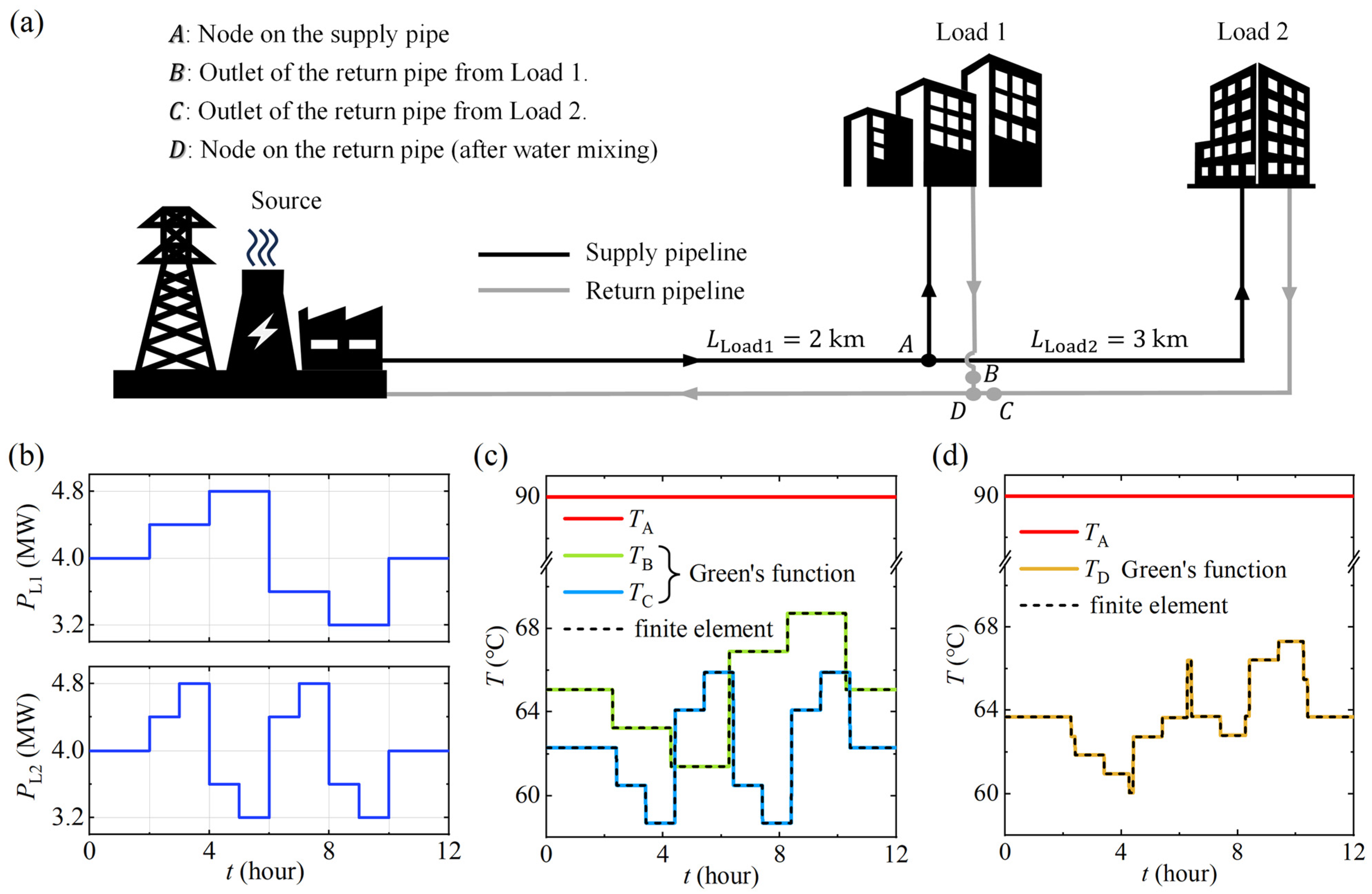
2.3.2. Semi-Infinite 1D Pipe with a Fixed Endpoint Temperature

In district heating systems, controlling the inlet temperature of pipelines is a widely adopted operational strategy. In such cases, it is necessary to model the pipeline using fixed endpoint temperature boundary conditions for a semi-infinite domain. When the endpoint temperature is fixed at $T\left(0,t\right)=0$, the Green’s functions for Equations (1) and (9) can be derived using the method of images. The principle of this method is to introduce a virtual negative image source in the $x<0$ region for each real heat source in $x>0$, which ensures that the boundary condition $T\left(0,t\right)=0$ is satisfied. The resulting Green’s function for Equations (1) and (9) is

$$G\left(x,t;\xi ,\tau \right)={\displaystyle \frac{1}{\sqrt{4\pi \alpha \left(t-\tau \right)}}}\left[\mathrm{e}\mathrm{x}\mathrm{p}\left(-{\displaystyle \frac{{\left(x-\xi \right)}^2}{4\alpha \left(t-\tau \right)}}\right)-\mathrm{e}\mathrm{x}\mathrm{p}\left(-{\displaystyle \frac{{\left(x+\xi \right)}^2}{4\alpha \left(t-\tau \right)}}\right)\right].$$

(11)

The Green’s function given by Equation (11) can also be used to calculate the temperature distribution under non-zero boundary conditions $T\left(0,t\right)=T_1\ne 0$. In this case, we define a new variable $T^{\prime }=T-T_1$, which satisfies $T^{\prime }\left(0,t\right)=0$. Using Equations (3) and (11), $T^{\prime }\left(x,t\right)$ is given by

$$T^{\prime }\left(x,t\right)={\int }_0^{\infty }G\left(x,t;\xi ,0\right)T^{\prime }\left(\xi ,0\right)\hspace{0.17em}\mathrm{d}\xi +{\int }_0^t{\int }_0^{\infty }G\left(x,t;\xi ,\tau \right)Q\left(\xi ,\tau \right)\hspace{0.17em}\mathrm{d}\xi \hspace{0.17em}\mathrm{d}\tau .$$

(12)

The original temperature distribution is then recovered via $T=T^{\prime }+T_1$:

$$\begin{array}{ll}T\left(x,t\right)=T_1+& {\int }_0^{\infty }G\left(x,t;\xi ,0\right)\left[T\left(\xi ,0\right)-T_1\hspace{0.17em}\right]d\xi \\ & \hspace{1em}+{\int }_0^t{\int }_0^{\infty }G\left(x,t;\xi ,\tau \right)Q\left(\xi ,\tau \right)\hspace{0.17em}d\xi \hspace{0.17em}d\tau .\end{array}$$

(13)

2.4. High-Flow-Velocity Approximation

2.4.1. Transient States

In the previous sections, we analytically derived the Green’s functions of Equation (5) under both the periodic boundary condition (Equation (10)) and the fixed endpoint temperature condition (Equation (11)). These results provide analytical solutions for heat transfer in 1D pipelines with steady flow velocities.

However, in engineering applications, the flow velocity in main pipelines typically exceeds 1 m/s. Under such high-flow conditions, the contribution of advection to heat transfer significantly outweighs that of thermal diffusion. As a result, the heat diffusion term, $-\kappa {\displaystyle \frac{{\partial }^{2}T\left(x,t\right)}{\partial x^2}}$, can be safely neglected [13,26,27]. With this approximation, Equation (5) is simplified to:

$$\rho c{\displaystyle \frac{\partial T}{\partial t}}+\rho cv{\displaystyle \frac{\partial T}{\partial x}}+{\displaystyle \frac{\mu \left(T-T_0\right)}{A}}=Q.$$

(14)

Equation (14) is a first-order PDE, which is much simpler than Equation (5). To solve for its Green’s functions, we first introduce the relative temperature $\mathrm{\Delta }T=T-T_0$ to eliminate the inhomogeneous term $\mu T_0/A$ on the left-hand side of the equation:

$$\rho c{\displaystyle \frac{\partial \mathrm{\Delta }T}{\partial t}}+\rho cv{\displaystyle \frac{\partial \mathrm{\Delta }T}{\partial x}}+{\displaystyle \frac{\mu }{A}}\mathrm{\Delta }T=Q.$$

(15)

The Green’s function for Equation (15) under the periodic boundary condition $T\left(x\right)=T\left(x+L\right)$ can then be obtained using Fourier series expansion:

$$G\left(x,t;\xi ,\tau \right)={\displaystyle \frac{1}{\rho cL}}{e}^{-{\displaystyle \frac{\mu }{A\rho c}}(t-\tau )}\sum _{n\in \mathbb{Z}}\delta \left(x-\xi -v\left(t-\tau \right)-nL\right).$$

(16)

This expression allows for the calculation of the temperature distribution in a closed-loop pipeline of total length $L$.

To simulate semi-infinite pipelines with given inlet temperatures, we also need the Green’s function for Equation (15) under the boundary condition $T\left(x,0\right)=0$. The Green’s function is given by

$$G\left(x,t;\xi ,\tau \right)={\displaystyle \frac{1}{\rho c}}{e}^{-{\displaystyle \frac{\mu }{A\rho c}}\left(t-\tau \right)}\delta \left(x-\xi -v\left(t-\tau \right)\right),$$

(17)

where $x\ge 0$ and $\xi >0$.

In the examples presented in Section 3, we will use Equations (16) and (17) for numerical calculations.

2.4.2. Steady State

Calculating the temperature distribution $T(x,t)$ using Equation (3) requires knowledge of the initial temperature distribution $T(x,0)$. However, in many practical applications, the system is often assumed to be in a steady state at $t=0$, and $T(x,0)$ is not directly known. In such cases, the initial temperature distribution $T(x,0)$ must be determined by solving the steady-state equation.

A steady state refers to a condition where the system remains unchanged over time. In this state, all heat source terms are time-independent, and the temperature distribution $T\left(x\right)$ is also time-invariant. Under steady-state conditions, Equation (15) simplifies to:

$$\rho cv{\displaystyle \frac{\partial }{\partial x}}\mathrm{\Delta }T+{\displaystyle \frac{\mu }{A}}\mathrm{\Delta }T=Q.$$

(18)

Equation (16) is a first-order partial differential equation in $x$ and can also be solved using the Green’s function method. In the following, we present the Green’s functions for Equation (16) under both periodic boundary conditions and fixed endpoint temperature boundary conditions.

Under periodic boundary conditions with a period of $L$, the Green’s function for Equation (16) is obtained as

$$G\left(x,\xi \right)={\displaystyle \frac{1}{\rho cvL}}\sum _{n\in \mathbb{Z}}{\displaystyle \frac{e^{i\frac{2\pi }{L}n\left(x-\xi \right)}}{i\frac{2\pi }{L}n+\frac{\mu }{\rho cvA}}}.$$

(19)

With this Green’s function, the steady-state temperature distribution $T\left(x\right)$ is given by

$$T\left(x\right)=T_0+\mathrm{\Delta }T(x)=T_0+{\int }_0^{L}G\left(x,\xi \right)Q\left(\xi \right)d\xi .$$

(20)

Under the boundary condition of a fixed endpoint temperature, the Green’s function for Equation (16) is given by

$$G\left(x,\xi \right)={\displaystyle \frac{1}{\rho cv}}{e}^{-{\displaystyle \frac{\mu }{\rho cvA}}\left(x-\xi \right)}H\left(x-\xi \right),$$

(21)

where $H\left(x-\xi \right)$ is the Heaviside step function, ensuring that $G\left(x,\xi \right)=0$ when $x<\xi$.

For a fixed endpoint temperature, $T\left(0\right)=T_1$, $T\left(x\right)$ can be obtained using the Green’s function in Equation (19) as

$$T\left(x\right)=T_0+\left(T_1-T_0\right)e^{-{\displaystyle \frac{\mu }{\rho cvA}}x}+{\int }_0^{\infty }G\left(x,\xi \right)Q\left(\xi \right)d\xi .$$

(22)

Here, $T\left(x\right)$ consists of two non-constant terms: The exponentially decaying term represents the influence of the boundary temperature in the presence of dissipation, while the integral term accounts for the impact of the heat source on the steady-state temperature distribution.

It is straightforward to verify that the solution $T\left(x\right)$ given by Equation (20) satisfies the required boundary conditions. As $x\to 0$, $T\left(x\right)\to T_1$, ensuring the correct endpoint temperature, and as $x\to \infty$, $T\left(x\right)\to T_0$, indicating that the temperature asymptotically approaches the ambient temperature.

In the examples presented in Section 3, we will use the Green’s functions given by Equations (17) and (19) for computing the steady-state temperature distributions.

3. Numerical Examples

In this section, we present two numerical examples to illustrate temperature distribution calculations using the Green’s function method. The first example involves a system with a single heating loop, where the water temperature distribution along the pipeline is calculated with respect to the heat source power. The second example examines the temperature distribution in a heating network. The variation in water temperature in the return pipeline is calculated as a function of user load, under the condition of a constant inlet water temperature. The flowchart of the numerical calculation is presented in Figure A1. In both cases, the results obtained using the Green’s function method are in excellent agreement with those from the finite element method, thus validating the reliability of the proposed computational approach.

3.1. Single Heating Loops

In this example, we apply the Green’s function method to calculate the temperature distribution in a closed-loop heating system. The model consists of an electric boiler, a booster pump, two heating pipelines, and a user heat load unit, as shown in Figure 2a. The electric boiler serves as the heat source, heating the water, while the booster pump is used to maintain a constant water flow velocity.

The model parameters are as follows: the lengths of the supply and return pipelines are $L_1=L_2=5$ km, corresponding to a total pipeline length of $L=L_1+L_2=10$ km. The heat dissipation coefficient and cross-sectional area of the pipeline are set to $\mu =2.8$ W/(m∙K) and $A=0.05$ m², respectively. The water flow velocity is $v=2$ m/s, and the ambient temperature is $T_0=0$°C. The electric boiler’s heating power $P_{\mathrm{S}}$ varies over time, as depicted in Figure 2b, while the user heat load power remains constant at $P_{\mathrm{L}}=8$ MW. It is assumed that the density, specific heat capacity, and thermal conductivity of water are temperature-independent, with values of $\rho =1000$ kg/m³, $c=4200$ J/(kg·K), and $\kappa =0.7$ W/(m·K). The system is assumed to be in a steady state at $t=0$.

Given that the flow velocity is significantly higher than the thermal diffusion speed, we neglect the thermal diffusion term in Equation (5) based on the discussion in Section 2.4 and instead employ Equations (15) and (18) for numerical calculations. Assuming that the heat source is located at $x=0$ and the user heat load is at $x=L_1$, the heat source terms corresponding to external heating and user heat load can be expressed as $Q_1=P_{\mathrm{s}}\delta \left(x\right)/A$ and $Q_2=-P_{\mathrm{L}}\delta \left(x-L_1\right)/A$, respectively.

Since the system is in a steady state at $t=0$, we first determine the initial temperature distribution $T\left(x,0\right)$ using the steady-state equation (Equation (18)) along with its Green’s function under periodic boundary conditions (Equation (19)). After that, we compute the time-dependent temperature distribution $T\left(x,t\right)$ using the transient equation (Equation (15)) and the corresponding Green’s function under periodic boundary conditions (Equation (16)). The flowchart of the simulation is shown in Figure A1.

The solid lines in Figure 2c depict the inlet and outlet temperatures of both the supply and return pipelines as functions of time. For validation, we also performed the same calculations using the finite element method, with the results shown as dashed lines in Figure 2c. The results obtained from both methods are in perfect agreement, validating the numerical reliability of the Green’s function approach. Furthermore, under identical hardware conditions, the Green’s function method completed the computation in 2.4 s, compared to 11.8 s required by the finite element method, demonstrating a significant improvement in computational efficiency.

3.2. Heating Networks

The following numerical example considers a heating network consisting of two parallel user load units. As illustrated in Figure 3a, the main supply pipeline bifurcates at node A, distributing heat to user loads Load 1 and Load 2, while the return pipelines converge at node D. The return pipelines merge at node D. The numerical method used in this example can be readily extended to more complex networks incorporating additional heat loads.

The model parameters are as follows: The supply and return pipeline lengths for Load 1 are both $L_{\mathrm{L}\mathrm{o}\mathrm{a}\mathrm{d}1}=2$ km, while those for Load 2 are $L_{\mathrm{L}\mathrm{o}\mathrm{a}\mathrm{d}2}=3$ km. The cross-sectional area of the branch pipelines is $A=0.025$ m², the heat dissipation coefficient is $\mu =4$ W/(m∙K), and the water flow velocity is $v=2$ m/s. The heat load powers $P_{\mathrm{L}1}$ and $P_{\mathrm{L}2}$ vary independently over time, following the curves shown in Figure 3b. The water temperature at node A is kept constant at $T_{\mathrm{A}}=90 °\mathrm{C}$, and the ambient temperature is $T_0=0 °\mathrm{C}$. The density, specific heat capacity, and thermal conductivity of water are assumed to be $\rho =1000$ kg/m³, $c=4200$ J/(kg·K), and $\kappa =0.7$ W/(m·K), respectively. The system is in a steady state at $t=0$.

The numerical calculations in this example are also based on Equations (15) and (18). Since the temperature at node A is constant, we utilize the Green’s functions for boundary conditions with fixed endpoint temperatures (Equations (17) and (21)) for both transient and steady-state analyses. The computational procedure is as follows: First, the initial temperature distributions of the two heating branches, $T_{\mathrm{L}\mathrm{o}\mathrm{a}\mathrm{d}1}\left(x\right)$ and $T_{\mathrm{L}\mathrm{o}\mathrm{a}\mathrm{d}2}\left(x\right)$, are obtained using the steady-state Equation (18) and its corresponding Green’s function (21). Then, the outlet temperatures of the return pipelines, $T_{\mathrm{B}}$ and $T_{\mathrm{C}}$, are computed as functions of time using the transient Equation (15) and its corresponding Green’s function (17). Finally, the mixed temperature at node D is determined as a weighted average of $T_{\mathrm{B}}$ and $T_{\mathrm{C}}$ and tracked over time. The results are shown as solid lines in Figure 3c,d. The flowchart of the simulation is shown in Figure A1.

To validate the reliability of our calculations, we repeated the computations using the finite element method, with the results shown as dashed lines in Figure 3c,d. As evident from the comparison, the results obtained from both methods are in perfect agreement, confirming the accuracy and reliability of the Green’s function approach.

4. Conclusions

In this work, we introduced a Green’s-function-based approach for simulating the temperature distribution in district heating networks. By transforming the heat conduction equation into a solvable form, we derived the analytical Green’s functions under both periodic and fixed endpoint temperature boundary conditions, establishing a unified mathematical foundation for analyzing thermal propagation in complex pipeline networks.

The methodology was systematically validated through two building-block examples: a single-loop heating system and a multi-user heating network with distributed thermal loads. In both scenarios, the Green’s function approach produced results consistent with those obtained from finite element simulations, demonstrating its high accuracy and reliability. In addition, benchmark comparisons showed that, under identical hardware conditions, the Green’s function method required only about one-fifth of the computation time compared to the finite element method, confirming its outstanding computational efficiency.

Compared to traditional numerical methods, the Green’s function method offers key advantages, including reduced computational complexity and a clear causal relationship between heat sources and temperature distributions. This approach not only improves the efficiency of heating network simulations but also provides deeper insights into system dynamics. Our findings highlight the potential of Green’s functions as a powerful analytical framework for optimizing district heating systems and integrating renewable energy sources.

Future work will focus on extending this method to more complex heating networks, incorporating time-dependent boundary conditions, and exploring its applications in practical energy management scenarios.

References

1. IPCC. Summary for Policymakers. In Climate Change 2023: Synthesis Report; Lee, H., Romero, J., Eds.; IPCC: Geneva, Switzerland, 2023; pp. 1–34. [Google Scholar]
2. Delbeke, J.; Runge-Metzger, A. The Paris Agreement. In Towards a Climate-Neutral Europe, 1st ed.; Delbeke, J., Vis, P., Eds.; Routledge: London, UK, 2019; pp. 24–45. [Google Scholar]
3. U.S. Energy Information Administration-EIA-Independent Statistics and Analysis. Available online: https://www.eia.gov/consumption/residential/data/2020/index.php (accessed on 29 December 2024).
4. Van de Graaf, T. International energy agency. In Handbook of Governance and Security, 1st ed.; Sperling, J., Ed.; Edward Elgar Publishing: London, UK, 2014; pp. 489–503. [Google Scholar]
5. IRENA International Renewable Energy Agency, Power to Heat and Cooling: Status. Available online: https://www.irena.org/Innovation-landscape-for-smart-electrification/Power-to-heat-and-cooling/Status (accessed on 29 December 2024).
6. Tracking Clean Energy Progress 2023-Analysis-IEA. Available online: https://www.iea.org/reports/tracking-clean-energy-progress-2023 (accessed on 29 December 2024).
7. Liu, S.; Guo, Y.; Wagner, F.; Liu, H.; Cui, R.Y.; Mauzerall, D.L. Diversifying heat sources in China’s urban district heating systems will reduce risk of carbon lock-in. Nat. Energy 2024, 9, 1021–1031. [Google Scholar] [CrossRef]
8. Kuntuarova, S.; Licklederer, T.; Huynh, T.; Zinsmeister, D.; Hamacher, T.; Perić, V. Design and simulation of district heating networks: A review of modeling approaches and tools. Energy 2024, 305, 132189. [Google Scholar] [CrossRef]
9. Pans, M.A.; Claudio, G.; Eames, P.C. Modelling of 4Th generation district heating systems integrated with different thermal energy storage technologies—Methodology. Energy Convers. Manag. 2023, 276, 116545. [Google Scholar] [CrossRef]
10. Chen, J.; Lv, H.; Ding, L.; Zhang, K.; Lai, Z.; Chenglong, H. Quasi-dynamic modeling and simulation of district heating systems: A Laplace Transform-Based Approach. Energy Rep. 2024, 11, 2794–2804. [Google Scholar] [CrossRef]
11. Dalla Rosa, A.; Li, H.; Svendsen, S. Modeling transient heat transfer in small-size twin pipes for end-user connections to low-energy district heating networks. Heat. Transf. Eng. 2013, 34, 372–384. [Google Scholar] [CrossRef]
12. Sartor, K.; Dewalef, P. Experimental validation of heat transport modelling in district heating networks. Energy 2017, 137, 961–968. [Google Scholar] [CrossRef]
13. Schweiger, G.; Larsson, P.; Magnusson, F.; Lauenburg, P.; Velut, S. District heating and cooling systems–Framework for Modelica-based simulation and dynamic optimization. Energy 2017, 137, 566–578. [Google Scholar] [CrossRef]
14. Van der Heijde, B.; Aertgeerts, A.; Helsen, L. Modelling steady-state thermal behaviour of double thermal network pipes. Int. J. Therm. Sci. 2017, 117, 316–327. [Google Scholar] [CrossRef]
15. Zhang, S.; Gu, W.; Yao, S.; Lu, S.; Zhou, S.; Wu, Z. Partitional decoupling method for fast calculation of energy flow in a large-scale heat and electricity integrated energy system. IEEE Trans. Sustain. Energy 2020, 12, 501–513. [Google Scholar] [CrossRef]
16. Pass, R.Z.; Wetter, M.; Piette, M.A. A thermodynamic analysis of a novel bidirectional district heating and cooling network. Energy 2018, 144, 20–30. [Google Scholar] [CrossRef]
17. Guelpa, E.; Verda, V. Compact physical model for simulation of thermal networks. Energy 2019, 175, 998–1008. [Google Scholar] [CrossRef]
18. Stevanovic, V.D.; Zivkovic, B.; Prica, S.; Maslovaric, B.; Karamarkovic, V.; Trkulja, V. Prediction of thermal transients in district heating systems. Energ. Convers. Manag. 2009, 50, 2167–2173. [Google Scholar] [CrossRef]
19. Denarie, A.; Aprile, M.; Motta, M. Heat transmission over long pipes: New model for fast and accurate district heating simulations. Energy 2019, 166, 267–276. [Google Scholar] [CrossRef]
20. Jackson, J.D. Classical Electrodynamics, 3rd ed.; John Wiley & Sons: Hoboken, NJ, USA, 1998; p. 39. [Google Scholar]
21. Fetter, A.L.; Walecka, J.D. Green’s Functions and Field Theory (Fermions). In Quantum Theory of Many-Particle Systems, 1st ed.; McGraw-Hill: New York, NY, USA, 1971; pp. 64–82. [Google Scholar]
22. Cole, K.D.; Beck, J.V.; Haji-Sheikh, A.; Litkouhi, B. Introduction to Green’s Functions. In Heat Conduction Using Green’s Functions, 2nd ed.; Taylor and Francis: London, UK, 2011; pp. 1–46. [Google Scholar]
23. Beck, J.V. Green’s function solution for transient heat conduction problems. Int. J. Heat. Mass. Tran. 1984, 27, 1235–1244. [Google Scholar] [CrossRef]
24. Cole, K.D. Fast-converging series for heat conduction in the circular cylinder. J. Eng. Math. 2004, 49, 217–232. [Google Scholar] [CrossRef]
25. Cole, K.D.; Yen, D.H. Green’s functions, temperature and heat flux in the rectangle. Int. J. Heat. Mass. Tran. 2001, 44, 3883–3894. [Google Scholar] [CrossRef]
26. Giraud, L.; Bavière, R.; Vallée, M.; Paulus, C. Presentation, validation and application of the District Heating Modelica library. In Proceedings of the 11th International Modelica Conference, Versailles, France, 21 September 2015. [Google Scholar]
27. Van der Heijde, B.; Fuchs, M.; Ribas Tugores, C.; Schweiger, G.; Sartor, K.; Basciotti, D.; Müller, D.; Nytsch-Geusen, C.; Wetter, M.; Helsen, L. Dynamic equation-based thermo-hydraulic pipe model for district heating and cooling systems. Energ. Convers. Manag. 2017, 151, 158–169. [Google Scholar] [CrossRef]
Figure 1. Schematic diagram of a district heating network. The red peak represents a heat pulse originating from the central heat source and propagating through the supply pipeline, while the blue valleys represent cooling pulses generated by heat consumers and traveling through the return pipeline.
Energies 18 02627 g001
Figure 2. (a) Schematic diagram of the closed-loop heating system analyzed in Section 3.1. (b) Time-dependent variation of the boiler’s heating power P S and P L 2 . (c) Inlet and outlet temperatures of the supply and return pipelines as functions of time, computed using the Green’s function method (solid lines) and the finite element method (dashed lines).
Energies 18 02627 g002
Figure 3. (a) Schematic diagram of a heating network with two heat load units. (b) Time-dependent variation of the heat load powers P L 1 . (c) Outlet temperatures T A and T B as functions of time, computed using the Green’s function method (solid lines) and the finite element method (dashed lines). The red line represents the temperature of node A for reference. (d) Temperature of node D as a function of time, calculated using the Green’s function method (solid lines) and the finite element method (dashed lines). The red line indicates the temperature of node A for reference.
Energies 18 02627 g003
Disclaimer/Publisher’s Note: The statements, opinions and data contained in all publications are solely those of the individual author(s) and contributor(s) and not of MDPI and/or the editor(s). MDPI and/or the editor(s) disclaim responsibility for any injury to people or property resulting from any ideas, methods, instructions or products referred to in the content.