Abstract
In order to improve the trading efficiency of virtual power plants (VPPs) participating in the market of multi-type auxiliary services under the gaming environment, an initial trading price setting method based on the information of VPPs’ response characteristics and real-time supply and demand changes is proposed to accelerate the convergence speed of the game. Firstly, a master–slave game trading model is established based on the reference auxiliary service pricing, which consists of a tariff coefficient and a basic tariff. Secondly, the tariff coefficient model is constructed based on response information, including response rate, quality, and reliability. Again, the basic tariff model is constructed based on the real-time supply and demand situation and the real-time grid tariff. Finally, the effectiveness of the proposed method in accelerating the convergence speed of the game is verified by analyzing 12 VPPs under the three auxiliary service scenarios of peaking, frequency regulation, and reserve.
1. Introduction
With the global energy transition, distributed energy resources (DERs) such as wind power, photovoltaic, energy storage, and flexible loads are developing rapidly, but the diversity of geographic locations, operating characteristics, and response characteristics of various DERs poses serious challenges to the safe operation of the power grid and trading in the power market [1,2,3]. As a new type of energy aggregation mode, virtual power plants (VPPs) can collaboratively aggregate geographically dispersed DERs and optimize their regulation through advanced information and communication technologies, which can aggregate various types of resources to participate in electricity and energy market transactions, while providing multiple high-quality ancillary services to the power system [4,5,6,7]. However, the electricity market environment inherently constitutes a competitive gaming environment with multiple decision-making entities [8,9,10], making the use of game theory to study VPPs trading and scheduling one of the mainstream approaches.
Current research extensively employs various game-theoretic frameworks, such as master–slave games and non-cooperative games, to analyze the interactive behavior between grid operators and VPPs. For example, references [11,12,13] utilize Stackelberg game theory to construct interaction models between multiple VPPs and the grid, considering the interests and demands of different subjects. These models effectively achieve collaborative optimization among VPPs and grid interaction. Reference [14] proposes a Stackelberg game-based optimization platform for electricity trading and scheduling, facilitating market participation of VPPs. In addition, other game theories have been used to conduct research. For example, references [15,16] employ dynamic games to develop day-ahead market optimization models for multi-VPP systems, enabling optimal benefit allocation under complex gaming scenarios. Although all of the above studies have adopted the ideas of game theory to solve the problems related to VPPs, the initial tariffs of the game are generally set empirically. However, due to the different types of resources aggregated by different VPPs, there is a gap in their overall response characteristics. If the detailed information of various types of VPPs and the grid side is not considered in the initial tariff setting, it will lead to a large deviation between initial and final clearing price, which increases the number of interactions between multiple VPPs and the grid, i.e., it increases the game iteration and computation time and, thus, reduces the efficiency of market clearing.
In addition, there are also related studies on initial value setting in game models. Reference [17] introduces a novel multi-entity distributed collaborative optimization strategy under a Stackelberg framework to address energy pricing challenges. Reference [18] applies a two-layer Stackelberg game to consider the impact of distributed coordination signals on the selection of virtual power plant members. Reference [19] proposes a two-stage game model for guiding the peer-to-peer energy trading pricing and deployment strategies for VPPs in order to charge users for shared services. Although the above reference on the initial value setting of the game model considers the relevant parameters and information, it is not comprehensive enough to consider the response characteristics of VPPs. Generally speaking, VPPs are greatly affected by the incentive tariffs when participating in the auxiliary service market, and if the incentive tariffs set in the initial stage of the game are not reasonable, the response of VPPs in the subsequent stages will be affected. Therefore, if the response characteristics of VPPs are included in the initial tariff setting at the initial stage, the speed of the game can be effectively improved.
Considering the above studies, this paper argues that the reference auxiliary service tariff can be set as the initial tariff of the game model by combining the response information of VPPs and the real-time information of the power grid in order to realize the fast convergence of the game trading model. Our hierarchical game framework positions the trading center as the leader and multiple VPPs as followers. Based on the master–slave game model, a new reference auxiliary service tariff setting method is proposed to improve the game efficiency and promote the interaction between each virtual power plant and the trading center. The method takes into account more comprehensive information, such as the response of each virtual power plant and the real-time supply and demand changes in the power grid, and constructs a reference auxiliary service tariff model that contains the tariff coefficient part and the basic tariff part, i.e., the product of the two parts. The tariff coefficient part is set for the virtual power plant with different response information, while the basic tariff part is set in relation to the power supply and demand relationship and the grid tariff. This setting method can not only incentivize virtual power plants with different response information to participate in market transactions and dispatch response actively but also reflect the actual operating costs of each subject in real-time, which can effectively reduce the number of iterations and time of the game, and improve the efficiency of market clearance.
2. System Model
2.1. Trading Center
The trading center pays incentive fees to multiple types of virtual power plants in order to meet the stable operation of the grid, which can be expressed as
where is the total incentive fee to be paid by the trading center; is the auxiliary service tariff issued by the trading center; is the total response of the virtual power plant at time t.
The reference auxiliary tariff set by the trading center shall satisfy the following constraints.
where and are the minimum and maximum values of the auxiliary tariff, respectively.
2.2. Virtual Power Plant
Economic modeling of various types of virtual power plants includes incentive benefits, power purchase costs, micro-gas turbine costs, energy storage costs, and interruptible load costs, which can be expressed as
where is the auxiliary service response power of the j-th VPP at time t; and are the selling tariff and purchasing tariff with the grid, respectively; and are the power sold and power purchased with the grid by the j-th VPP, respectively; denotes the set of resources contained in the j-th VPP; is the micro-gas turbine costs; is the energy storage costs; is the interruptible load costs; is the output power of the i-th micro-gas turbine; is the charging or discharging power of the i-th energy storage; is the interrupt power of the i-th interruptible load; ,, are the cost coefficient of micro-gas turbine; is the cost coefficient of energy storage; is greater than 0 for discharging, and is less than 0 for charging; and is the interruption cost coefficient.
The VPP needs to satisfy the power balance constraints and the operational constraints of each type of resource when responding to the price. The constraints can be expressed as
where and are the output power of the i-th wind power and photovoltaic in the j-th VPP at time t, respectively; is the predicted value of the load at time t; is the upper limit of the output power of the micro-gas turbine; and is the upper and lower limit of the creep rate of the micro-gas turbine, respectively; and is the upper and lower limit of the output power of the energy storage, respectively; is the charge state of the energy storage at time t; and is the charging and discharging power of the energy storage, respectively; and is the charge and discharging efficiency of the energy storage, respectively; and is the upper and lower limit of the charge state of the energy storage, respectively; , , and is the upper and lower limit of the interruptible load, the distributed wind power and distributed photovoltaic, respectively.
3. Problem Formulation
In general, participants, strategies, and utility functions are the three basic elements of a game model. In the Stackelberg game process, the auxiliary service trading center and VPP, as participants, play the roles of leader and follower. As a leader, the trading center’s strategy is tariff setting with the goal of minimizing the total incentive cost by optimizing the tariff as a decision variable. As a follower, the VPP’s strategy is to optimize the allocation of response power, with the goal of maximizing its own revenue by optimizing decision variables such as distributed power output, storage charging and discharging, and interruptible load response power.
During the first gaming process, the power dispatch and trading center determines the type of auxiliary services required and the amount of power demanded based on the real-time operating status of the grid and gives priority to the release of pricing strategies. Then, each VPP calculates the optimal response power based on the price signal and feeds the result back to the trading center. If the total response power deviates from the demand beyond the threshold, the trading center further updates the tariff strategy, triggering a new round of gaming. In the subsequent game, the trading center can guide the power dispatch of multiple VPPs through price optimization, and the power dispatch decisions of multiple VPPs will also affect trading with the ancillary services market. Finally, when the joint solution of tariff strategy and response power satisfies the Nash equilibrium condition (i.e., either participant cannot unilaterally change the strategy to improve its own revenue), the game reaches a stable state, and the trading center generates the clearing tariff and completes the settlement accordingly. The transaction interaction process between the two is sequential, in line with the master–slave dynamic game, and the detailed process of the game is shown in Figure 1.
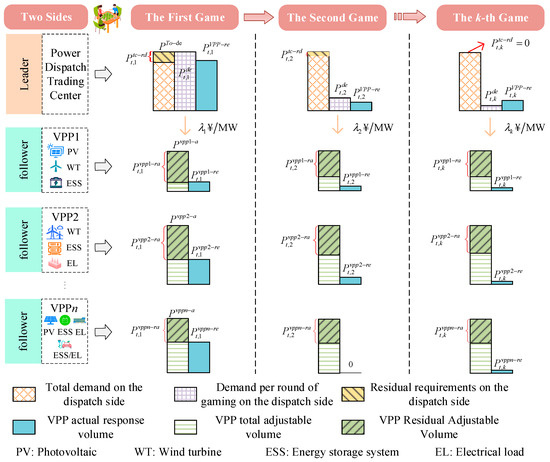
Figure 1.
Detailed process of the Stackelberg game.
However, the initial tariffs used in the above master–slave dynamic game are usually set empirically, without taking into account the different responses of VPPs under the tariff incentives and the real-time supply and demand changes in the grid. This makes it difficult for the responses of VPPs to meet the requirements of the auxiliary service center in setting the initial tariff strategy, leading to a large deviation between the initial clearing price and the final clearing price, increasing the number of iterations and calculation time of the game, and decreasing the efficiency of market clearing. The efficiency of market clearing can be improved if the power supply and demand information and the response of each VPP are more comprehensively considered when setting the tariff at the beginning of the game, so that the deviation between the initial tariff and the final market clearing tariff is minimized. Based on this idea, a reference auxiliary service tariff that takes into account the response information of each VPP and the real-time supply and demand change information of the grid is introduced, which further improves the convergence speed and game efficiency at the early stage of the game. The reference auxiliary service tariff is used to motivate the virtual power plants with different response information to actively participate in the market transaction and dispatch response during the dynamic game process, and at the same time, reflect the actual benefits of both parties in the game, and promote the interaction between the VPPs and the trading center, and the proposed new model is shown as follows.
3.1. Leader Trading Center Game Model
3.1.1. Trading Center Strategy
The gaming strategy adopted by the trading centers is to set incentive fees for VPP for each time period, denoted as
3.1.2. Trading Center Utility Function
The utility function is to minimize the total incentive cost paid, which can be expressed as
where is the reference auxiliary tariff at time t.
3.1.3. Trading Center Strategy Space
The constraint satisfied by the reference auxiliary tariff set by the trading center is given in detail in Section 2.1, which constitutes the strategy space of the trading center, denoted as .
3.2. Follower VPP Game Model
3.2.1. VPP Strategy
The game strategy for VPP is the power of the response to the trading center, denoted as .
3.2.2. VPP Utility Function
The utility function is to maximize the VPP’s own revenue, which can be expressed as
3.2.3. VPP Strategy Space
The constraints that the VPP needs to satisfy when responding to prices are given in detail in Section 2.2, and these constraints constitute the strategy space of the VPP, denoted as .
3.3. Master–Slave Game Modeling
Based on Section 3.1 and 3.2, the master–slave game model for trading center and multi-VPPs is developed as follows:
The reference auxiliary tariff at time t consists of two parts, the tariff coefficient part and the basic tariff part , denoted as
Therefore, the tariff coefficients and basic tariffs need to be modeled, and the modeling process will be developed in the following section. The general framework diagram of this paper is shown in Figure 2.
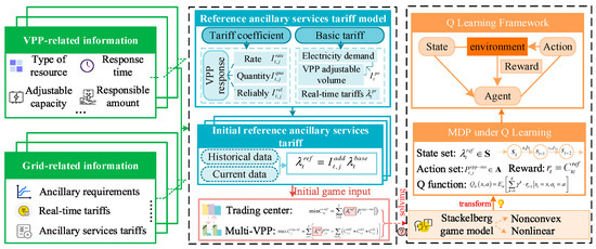
Figure 2.
General framework diagram.
4. Tariff Coefficient Model Based on VPP Response Characteristics
4.1. Components of Tariff Coefficient Model
Tariff coefficients are first modeled based on the information of each VPP. The of VPPs with different own information is different, for example, when the VPP has a better climbing ability or a higher electrical energy charging and discharging ability at moment t, etc., the VPP will have a larger , and vice versa, the will be smaller. Therefore, the performance of different virtual power plants in actual operation is quantitatively evaluated and compared by considering the response information of each virtual power plant, such as response speed, duration, available capacity, etc., in the formulation of tariff coefficients. The quantification of response information in current research mainly focuses on the three dimensions of time, effect, and stability, while other dimensions have less influence on the quantification of virtual power plant response information, and more dimensions will lead to an increase in computational complexity. Therefore, this paper constructs a tariff coefficient model containing three influencing factors. The influencing factors include the response speed, response quality, and response reliability of VPP, which correspond to the above three dimensions, while the other influencing factors can be ignored due to their small impact on the quantification of the corresponding information of the virtual power plant. The response rate focuses on measuring the ability of the VPP to respond quickly to grid dispatch commands or market signals. Response quality focuses on reflecting the degree of consistency between the actual response effect of the VPP and the auxiliary demand when providing auxiliary services. Response reliability focuses on reflecting the probability and ability of the VPP to offer auxiliary services stably under various operating conditions and market demands.
Higher incentive gains can only be achieved if the VPP has both fast responsiveness, high-quality output, and reliable response. The multiplication form is used here not only to intuitively reflect the contribution of each influencing factor to the total incentive effect but also to model certain nonlinear cost–benefit relationships better. At this point, the of the j-th VPP is modeled as
where , , and denote the response rate, response quality, and response reliability of the VPP, respectively.
The modeling of each of the three parameters is described below.
4.2. Response Rate
Considering that the effect of response time on the reference auxiliary service tariff is nonlinear, the larger the deviation of the actual response time from the set standard time, the faster the reference auxiliary service tariff becomes smaller. Therefore, a quadratic function was used to fit the segment in , and the results are shown in Equation (21).
where is the actual response time of the j-th VPP at time t, and are the given reference time and maximum allowable time, respectively. Since lags behind the pricing time, it can be replaced by the historical value in practical applications.
4.3. Response Quality
Considering that the response quality of VPP is affected by the tariff, the response quality of VPP is expressed here as the ratio of the actual response power to the total adjustable quantity under different reference auxiliary service tariffs, as shown in Equation (22).
where is the theoretical response quality of the VPP; is the actual response power of the j-th VPP; is the total adjustable quantity; and represents the response quality of the VPP as a function of the tariff.
Different VPPs respond differently under different price incentives, and the VPP response is nonlinearly related to price, making it difficult to evaluate the response quality of VPPs comprehensively. In addition, the incentive price may cause VPPs to make subjective judgments, further increasing the difficulty of evaluating the response quality of different VPPs. Here, the static response quality is proposed. denotes the statistical characteristics of the set consisting of the historical VPP response and the historical optimal reference auxiliary service tariff, including the arithmetic mean characteristics of the response quality and the characteristics of the variation coefficient , in order to represent the level and fluctuation of the VPP response performance, the modeling process is shown in Equations (23)–(25).
where is the standard deviation of the static response quality of the j-th VPP; the larger is, the better the responsiveness of the VPP to the incentive price; the larger is, the smaller the fluctuation of the VPP’s response to the incentive price; and the precision of the static response quality increases with the increase in the number of elements in the set .
Therefore, based on the construction of the static response performance model above, the actual response quality model of VPP can be transformed from Equations (22)–(27).
where and denote the corresponding weights of and .
4.4. Response Reliability
Response reliability is measured primarily by three factors, namely average annual unavailability, failure rate, and number of unplanned interruptions, the formula for which can be expressed as
where denotes the values of the above three factors in the response reliability of the j-th VPP in turn, which will be calculated based on statistical knowledge. denotes the weighting factor for response reliability. In addition, in order to ensure that the range of values is from 0 to 1, the data have been processed by the min-max normalization method, which is calculated as in Equation (29).
where is the value of the m-th influencing factor before normalization; is the total number of VPPs online at moment t; m = 1, 2, 3.
The average annual unavailability time measures the ability of the VPP to stay online and respond to grid demand most of the time. The computational model is shown in Equations (30)–(32).
where is the quantitative value of the factors affecting the annual mean unavailability time in the response reliability of the j-th VPP; is the annual mean unavailability time of the j-th VPP; and are the mean and standard deviation of the annual mean unavailability time of the j-th VPP, respectively.
The failure rate directly affects the power system’s trust in the reliability of the VPP, which is modeled in Equations (33)–(36).
where is the quantitative value of the factors affecting the failure rate in the response reliability of the j-th VPP; is the failure rate of the j-th VPP, which is expressed as the failure number under a specific operating time interval ; and are the mean and standard deviation of the failure rate of the j-th VPP.
The number of unplanned interruptions focuses on the emergency response capability of the VPP and the effectiveness of preventive measures, and it is calculated as modeled in Equations (37)–(39).
where is the quantitative value of the factors affecting the number of unplanned interruptions in the response reliability of the j-th VPP; is the number of unplanned interruptions of the j-th VPP; and are the mean and standard deviation of the number of unplanned interruptions of the j-th VPP, respectively. denotes the base value taken by the logarithm in the model for the number of unplanned interruptions.
5. Basic Tariff Model
In this subsection, the basic tariff is modeled. is related to the relationship between electricity supply and demand, as well as grid electricity price.
Specifically, can be composed of two parts, and , where is the incentive power price part affected by the power supply demand relationship, and is the part affected by the grid electricity price factor. The relationship between and is set to be logarithmic, and the relationship between and is set to be linear. Assuming that any of and converges to 0, also converges to 0. The basic tariff of the system at time t can be expressed as
can be expressed as
where and are the when the scheduling center needs the VPP to release and absorb power, respectively, which can be expressed as the ratio of the power demand to the adjustable power of the VPP at this time, i.e., ; and are the dischargable and rechargeable capacities of the j-th VPP at time t, respectively; and are the logic variables for the n-th VPP to participate in the scheduling, which take the values of .
can be expressed as
where is the combination of real-time electricity price and compensation price of energy storage resources; is the real-time electricity price of the grid; is the compensation price of energy storage resources in VPP dispatch, and the compensation price should be less than the real-time electricity price; is the revenue coefficient of dispatch VPP; is the compensation coefficient of the dispatch center for VPP with energy storage resources, and the coefficients take the values between 0,1.
6. Solution Algorithm
In order to minimize the costs paid by the trading centers and to minimize the number of price adjustment strategies, the selection will be made in descending order of VPP response. Therefore, the original complex nonlinear and nonconvex game problem can be formulated as an optimal choice of each VPP response, where the tariff coefficients of the VPPs need to be chosen to develop the pricing strategy. The pricing problem can be represented as a finite Markov decision process (MDP) whose outcome is partly controlled by the decision maker and partly stochastic. In this paper, this MDP is solved by the Q-learning algorithm. In the Q-learning framework, the MDP can be represented as
(1) State set : , indicates current ancillary services tariff .
(2) Action set : The action of the current state , indicates that each VPP response quantity .
(3) Reward : Indicates the negative value of the total incentive fee paid for the trading center.
(4) Action Value Functions : Evaluating the Quality of Action-State Pairs Using Cumulative Rewards as a Function of Action Values, expressed as follows:
where denotes the time step, denotes the strategy for mapping from states to actions, and denotes the discount rate of future rewards relative to the importance of current rewards.
The main objective of the pricing problem presented here is to maximize the action-value function, i.e., a set of optimal actions (each VPP response ), by finding the optimal policy , expressed as follows:
The Q-learning algorithm is used here to iteratively update the values of the action-value function through Bellman’s equation, expressed as follows:
In addition, the Q value can be updated by the following equation:
where denotes the extent to which the new Q-value can override the learning rate of the old Q-value
The algorithm’s flowchart is shown in Figure 3.
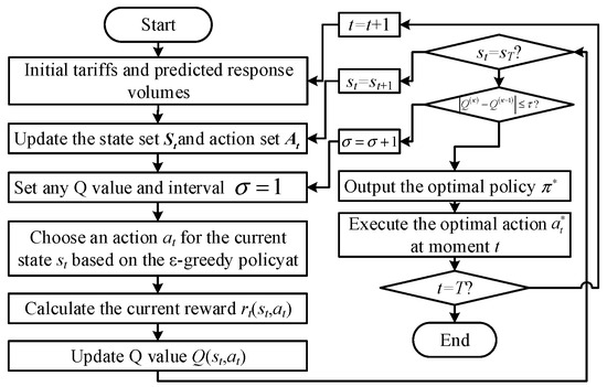
Figure 3.
Algorithm flowchart.
7. Case Study
7.1. Parameter Setting
In this subsection, the parameters of VPP-related information were first set. A total of 12 VPPs are participating in the market, of which 6 are used for peaking, 4 for frequency regulation, and 2 for reserve, and the adjustable capacity of each VPP is shown in Table 1. Secondly, 12 market scenarios are set up here, including intraday peaking, frequency regulation, and reserve. Among them, scenarios 1–6 are peaking markets, scenarios 7–10 are frequency regulation markets, and scenarios 11–12 are reserve markets. The specific information of each scenario is shown in Table 2.

Table 1.
Adjustable capacity of each VPP.
Table 2.
Power demand in each scenario.
7.2. Analysis of Reference Ancillary Services Tariff Modeling
This subsection analyses the above reference ancillary services tariff model, in order to verify the reasonableness and validity of the proposed model. The initial reference ancillary services tariff for each VPP under different scenarios is firstly given, as shown in Figure 4. Then, by simulating the 12 scenarios, the relationship between the power demand and the total response of VPPs under each scenario is also derived, as shown in Figure 5.
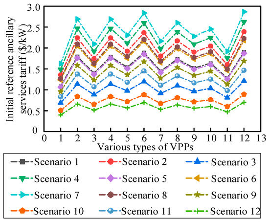
Figure 4.
Initial reference ancillary services tariff.
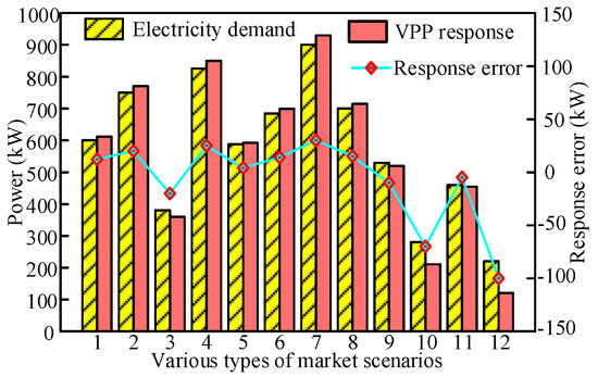
Figure 5.
Electricity demand and VPP response in each scenario.
As can be seen in Figure 4, the reference auxiliary service tariffs for each VPP vary across scenarios, with Scenario 7 having the highest average reference auxiliary service tariff and Scenario 4 the second highest, which is due to the fact that these two scenarios have the highest electricity demand, and setting higher reference auxiliary service tariffs can better incentivize the VPPs. In addition, both VPP6 and VPP12 have relatively high reference ancillary service tariffs in the same scenarios due to the higher tariff factor component of these two VPPs with better historical response. In Figure 5, the average error between the total response power volume of VPP and the electricity demand under the consideration of the reference auxiliary service tariff is 27.08 kW for the 12 kinds of scenarios, which is much smaller than the average value of the electricity demand of 576.5 kW. Although there is some error between the obtained VPP total response power and electricity demand, the trend is consistent, so the proposed model is reasonable and effective, and the reference auxiliary service tariff can be used as the initial tariff for the input of the game model.
7.3. Comparative Analysis of Response Under Different Tariffs
Two cases are designed here for comparison, respectively:
Case 1: The game model excluding reference ancillary service pricing;
Case 2: The game model incorporating reference ancillary service pricing.
(1) Comparative analysis of response errors under different cases
This subsection compares the responses to the above two scenarios. The obtained errors of the final response of the VPP with respect to the electricity demand under the 12 scenarios are shown in Figure 6. As can be seen from the figure, under the peaking demand scenarios (Scenarios 1–6), the average absolute error of the case 2 final response is 11.17 kW, while the average absolute error of the case 1 final response is 20.67 kW. This is due to the fact that under case1, the trading center is unable to fully grasp the re-responsiveness of various types of virtual power plants, which leads to the formulation of tariffs that are difficult to better meet the willingness of various types of virtual power plants to respond, and ultimately leads to a larger deviation. Except for Scenarios 3 and 6, the final response errors in case 2 are small. In Scenarios 3 and 6, the final response error of case1 is negative, i.e., the response fails to meet the demand. This indicates that by setting different reference auxiliary service tariffs, the VPPs can be better incentivized to respond to the demand and ensure that the trading demand is reached. In contrast, not considering the reference ancillary services tariff will affect the response of each VPP and reduce the efficiency of trading. This proves that the proposed model is highly accurate when oriented to peak demand. In the frequency-regulated demand scenarios (Scenarios 7–10), the average absolute error in the final response for case2 is 31 kW, while the average absolute error in the final response for case 1 is 14.75 kW. Although the final response error of the proposed model is larger, it is negative in both Scenario 9 and Scenario 10 when the reference ancillary service tariff is not considered. This demonstrates the high reliability of the proposed model under the frequency regulation scenario. This indicates that considering reference ancillary service tariffs can take into account the interests of all types of VPPs and ensure that demand is met, with higher reliability, while not considering reference ancillary service tariffs reduces reliability due to under-responsiveness because it fails to accurately take into account the response information of some VPPs. In the reserve demand scenarios (Scenarios 11–12), the average absolute error in final response for case 2 is 20.5 kW compared to 9.5 kW for case1. However, in Scenario 12, the response error for case1 is negative. This indicates that the proposed model has high reliability in the standby scenario as well. In conclusion, without considering the auxiliary service reference tariff, there is a situation where the demand cannot be met in time, whereas with the consideration of the auxiliary service reference tariff, all the scenarios can meet the demand although some of the scenarios have a large re-response error, which proves the validity of the proposed model.
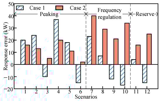
Figure 6.
Analysis of the response of different models in each scenario.
(2) Comparative analysis of each VPP response in the same scenario
In this paper, scenario 4 is used to analyze the response of each VPP under two cases, and the results are shown in Figure 7. The response volumes of VPPs 2, 3, 6, 8, and 12 are higher when the reference ancillary service tariff is considered than when it is not considered, and, in particular, the changes in VPPs 6 and 12 are more significant. This is due to the fact that the tariff coefficients of these VPPs are higher, while the other VPPs have lower response volumes than when the reference ancillary service tariff is not considered. However, the overall response error is ultimately lower when considering the reference auxiliary service tariff. This indicates that the reference auxiliary service tariff can better stimulate the response potential of each VPP, and the proposed model is superior.
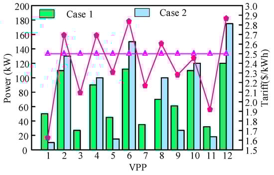
Figure 7.
Analysis of the response of each VPP in the same scenario.
(3) Comparative analysis of the same VPP response in different scenarios
The response of the same VPP in different scenarios is analyzed using VPP6, and the results are shown in Figure 8. As can be seen from the figure, in peaking scenarios 2, 4, and 6, the amount of response is higher when the reference ancillary service tariff is taken into account than when it is not, and the magnitude of the change is larger. In scenarios 1, 3, and 5, the amount of response is lower when the reference ancillary service tariff is considered than when it is not considered. This is due to the fact that the former has a higher demand for electricity, and it sets a larger reference ancillary service tariff, which ensures that the overall demand for electricity is met. This shows that the reference auxiliary service tariff proposed in this paper is more capable of ensuring that the trading demand is met.
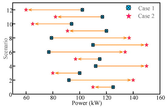
Figure 8.
Analysis of the response of the same VPP in different scenarios.
7.4. Comparative Analysis of the Gaming Process Under Different Tariffs
This subsection analyzes the game process with the above reference ancillary service tariff given as an input to the game model.
(1) Analysis of the game process of each VPP when considering the reference tariff in a single scenario
Firstly, Scenario 4 is taken as an object to analyze the game process of each VPP when considering and disregarding the reference auxiliary service tariff, based on the objective function of each participant, and the results of the analysis are shown in Figure 9. As can be seen from the figure, VPP12, VPP6, VPP2, and VPP10 show the largest increases, partly because of their larger responsive capacity, and partly because of the relatively high reference ancillary service tariffs given by the auxiliary service centers to these VPPs to ensure that the trading is completed. In addition, the number of iterations of the game equilibrium when the reference auxiliary service tariff is considered is 24, while the number of iterations when it is not considered is 45, which can be seen that the number of iterations used in the game is significantly reduced after the introduction of reference auxiliary service tariff. This shows the superiority and effectiveness of the reference auxiliary service tariff model proposed in this paper.
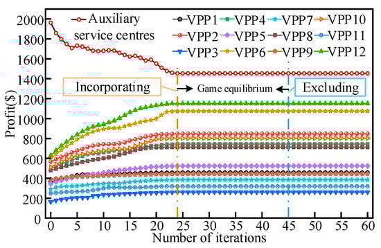
Figure 9.
Analysis of the gaming process of each VPP in scenario 4.
(2) Comparative analysis of the number of iterations and time used for game iterations with and without reference tariffs in all scenarios
From Figure 10 and Table 3, the average value of the number of iterations is 20 when the reference ancillary services tariff is considered, while it is 41 when it is not considered, and the iteration times are all faster when the reference ancillary services tariff is considered than when it is not considered. Introducing this reference tariff provides a better initial point for the subsequent game process, reduces the number of games (the number of price strategy adjustments), and, at the same time, makes the game iteration time much shorter, solving the problem that the game process requires VPP to respond many times, which leads to a higher number of game times and a longer game time.
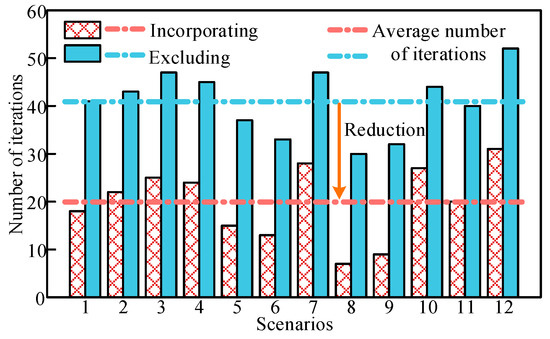
Figure 10.
Number of game iterations for each scenario.
Table 3.
Comparison of gaming iteration times across scenarios.
8. Conclusions
Considering the response rate, response quality, and response reliability information of various types of VPPs, as well as real-time power supply and demand changes and real-time grid tariff information, this paper constructs a reference auxiliary service tariff model with two parts: the tariff coefficient and the basic tariff. By introducing this reference auxiliary service tariff model into the master–slave game model, rapid convergence of the game model is realized. By analyzing the case, the following conclusions are obtained:
(1) The method proposed in this paper can effectively reduce the deviation between the initial tariff and the final market-clearing tariff, reduce the number of iterations of the game, improve the convergence speed of the game, and thus enhance the efficiency of market clearing.
(2) By setting different tariff coefficients for VPPs with different response characteristics, the different response potentials of various types of VPPs are stimulated, which can enable various types of VPPs to better respond to the provision of auxiliary services in terms of response volume, and help to enhance the efficiency of gaming transactions.
(3) The basic tariff, which is formulated based on the information of power supply and demand relationship and real-time grid tariffs, can be quickly adjusted according to the response of various types of VPPs, realizing the rapid updating of incentive tariffs in the gaming process, so as to more effectively promote the response of VPPs and ensure the balance of power supply and demand and the security and stability of power grids.
Author Contributions
Conceptualization, J.Y.; methodology, M.Z., X.G., T.W. and Y.W.; software, H.T.; validation, M.Z. and Y.W.; formal analysis, X.C.; resources, H.T.; writing—original draft preparation, J.Y. and X.C.; writing—review and editing, M.Z., X.G. and Y.W.; visualization, H.T. and Y.W.; supervision, M.Z., X.G., T.W. and Y.W.; funding acquisition, M.Z. and T.W. All authors have read and agreed to the published version of the manuscript.
Funding
This work was supported by the Science and Technology Project of SGCC (Research on testing and evaluating technology of virtual power plant operation capability for market interaction) (5400-202415213A-1-1-ZN).
Data Availability Statement
The original contributions presented in the study are included in the article material, further inquiries can be directed to the corresponding author.
Conflicts of Interest
Author Hongxun Tian was employed by the State Grid Shanxi Electric Power Company. The remaining authors declare that the research was conducted in the absence of any commercial or financial relationships that could be construed as a potential conflict of interest.
References
- Wang, T.; O’Neill, D.; Kamath, H. Dynamic Control and Optimization of Distributed Energy Resources in a Microgrid. IEEE Trans. Smart Grid 2015, 6, 2884–2894. [Google Scholar] [CrossRef]
- Viana, M.S.; Ramos, D.S.; Manassero Junior, G.; Udaeta, M.E.M. Analysis of the Implementation of Virtual Power Plants and Their Impacts on Electrical Systems. Energies 2023, 16, 7682. [Google Scholar] [CrossRef]
- Li, X.; Hu, C.; Luo, S.; Lu, H.; Piao, Z.; Jing, L. Distributed Hybrid-Triggered Observer-Based Secondary Control of Multi-Bus DC Microgrids Over Directed Networks. IEEE Trans. Circuits Syst. I Regul. Pap. 2025, 72, 2467–2480. [Google Scholar] [CrossRef]
- Camal, S.; Michiorri, A.; Kariniotakis, G. Optimal Offer of Automatic Frequency Restoration Reserve From a Combined PV/Wind Virtual Power Plant. IEEE Trans. Power Syst. 2018, 33, 6155–6170. [Google Scholar] [CrossRef]
- Shokouhinejad, H.; Guerra, E.C. Self-Scheduling Virtual Power Plant for Peak Management. Energies 2024, 17, 2705. [Google Scholar] [CrossRef]
- Yang, T.; Wang, J.; Liang, Y.; Xiang, C.; Wang, C. Economic Dispatch between Distribution Grids and Virtual Power Plants under Voltage Security Constraints. Energies 2023, 17, 117. [Google Scholar] [CrossRef]
- Shang, Y.; Li, D.; Li, Y.; Li, S. Explainable Spatiotemporal Multi-Task Learning for Electric Vehicle Charging Demand Prediction. Appl. Energy 2025, 384, 125460. [Google Scholar] [CrossRef]
- Zhang, W.; He, C.; Wang, H.; Qian, H.; Lin, Z.; Qi, H. Optimal Operation of Virtual Power Plants Based on Stackelberg Game Theory. Energies 2024, 17, 3612. [Google Scholar] [CrossRef]
- Wu, Y.; Lin, Z.; Liu, C.; Chen, Y.; Uddin, N. A Demand Response Trade Model Considering Cost and Benefit Allocation Game and Hydrogen to Electricity Conversion. IEEE Trans. Ind. Appl. 2022, 58, 2909–2920. [Google Scholar] [CrossRef]
- Jiang, L.; Yan, C.; Zhang, C.; Wang, W.; Wang, B.; Li, T. A Master–Slave Game Model of Electric Vehicle Participation in Electricity Markets under Multiple Incentives. Energies 2024, 17, 4290. [Google Scholar] [CrossRef]
- Chen, W.; Qiu, J.; Chai, Q. Customized Critical Peak Rebate Pricing Mechanism for Virtual Power Plants. IEEE Trans. Sustain. Energy 2021, 12, 2169–2183. [Google Scholar] [CrossRef]
- Wu, J.-K.; Liu, Z.-W.; Li, C.; Zhao, Y.; Chi, M. Coordinated Operation Strategy of Virtual Power Plant Based on Two-Layer Game Approach. IEEE Trans. Smart Grid 2025, 16, 554–567. [Google Scholar] [CrossRef]
- Zangeneh, A.; Shayegan-Rad, A.; Nazari, F. Multi-Leader–Follower Game Theory for Modelling Interaction between Virtual Power Plants and Distribution Company. IET Gener. Transm. Distrib. 2018, 12, 5747–5752. [Google Scholar] [CrossRef]
- Zhang, T.; Li, Y.; Yan, R.; Abu-Siada, A.; Guo, Y.; Liu, J.; Huo, R. A Master-Slave Game Optimization Model for Electric Power Companies Considering Virtual Power Plant. IEEE Access 2022, 10, 21812–21820. [Google Scholar] [CrossRef]
- Liu, R.; Chen, K.; Sun, G.; Lin, S.; Jiang, C. Bidding Strategy for the Virtual Power Plant Based on Cooperative Game Participating in the Electricity-Carbon Joint Market. Int. J. Electr. Power Energy Syst. 2024, 163, 110325. [Google Scholar] [CrossRef]
- Wang, Y.; Ai, X.; Tan, Z.; Yan, L.; Liu, S. Interactive Dispatch Modes and Bidding Strategy of Multiple Virtual Power Plants Based on Demand Response and Game Theory. IEEE Trans. Smart Grid 2016, 7, 510–519. [Google Scholar] [CrossRef]
- Shui, J.; Peng, D.; Zeng, H.; Song, Y.; Yu, Z.; Yuan, X.; Shen, C. Optimal Scheduling of Multiple Entities in Virtual Power Plant Based on the Master-Slave Game. Appl. Energy 2024, 376, 124286. [Google Scholar] [CrossRef]
- Esfahani, M.; Alizadeh, A.; Cao, B.; Kamwa, I.; Xu, M. Virtual Power Plant Formation Strategy Based on Stackelberg Game: A Three-Step Data-Driven Voltage Regulation Coordination Scheme. Appl. Energy 2025, 377, 124355. [Google Scholar] [CrossRef]
- Zeng, Y.; Wei, X.; Yao, Y.; Xu, Y.; Sun, H.; Kin Victor Chan, W.; Feng, W. Determining the Pricing and Deployment Strategy for Virtual Power Plants of Peer-to-Peer Prosumers: A Game-Theoretic Approach. Appl. Energy 2023, 345, 121349. [Google Scholar] [CrossRef]
Disclaimer/Publisher’s Note: The statements, opinions and data contained in all publications are solely those of the individual author(s) and contributor(s) and not of MDPI and/or the editor(s). MDPI and/or the editor(s) disclaim responsibility for any injury to people or property resulting from any ideas, methods, instructions or products referred to in the content. |
© 2025 by the authors. Licensee MDPI, Basel, Switzerland. This article is an open access article distributed under the terms and conditions of the Creative Commons Attribution (CC BY) license (https://creativecommons.org/licenses/by/4.0/).