Hierarchical Optimization Strategy for Integrated Water–Wind–Solar System Considering Load Control of Electric Vehicle Charging Stations

Abstract

For a high proportion of new energy with access to the grid, the typical random volatility of wind power and photovoltaic output greatly increases the peak load of the grid; in addition, the problem of wind and solar abandonment needs to be solved. This paper proposes the use of electric vehicle charging stations as new peak load resources to participate in grid dispatching. First, according to the actual operation and regulation characteristics of the load of EV charging stations, a refined regulation model enabling charging stations to participate in grid peak load regulation is established; then, combined with the deep peak load regulation model of hydropower units, in order to minimize system abandonment and minimize operating costs, a hierarchical optimization model for the joint peak load regulation of charging stations and hydropower deep regulation is established; finally, taking the actual power grid system as an example, a deep reinforcement learning algorithm is used to solve and analyze the problem, and the effectiveness of the scheme is verified. This study provides valuable insights into the coordinated optimization of electric vehicle charging stations and hydro–wind–solar systems for seamless integration into grid peak-shaving services.

1. Introduction

New energy generation technologies such as wind power and photovoltaic power have become effective solutions for alleviating the global energy crisis and environmental problems. According to statistics, the amount of electricity generated by renewable energy has increased rapidly in recent years [1]. With the continuous deepening of industrial structure adjustment in various countries, the demand for electricity has risen rapidly. Additionally, the balance between power supply and demand is facing great pressure [2].

The large-scale grid-connected operation of new energy sources such as wind power and photovoltaic power has injected a large amount of clean energy into the power grid. China’s wind power and photovoltaic installed capacity will exceed 1.2 billion kilowatts by 2030, and will grow to 3.6 billion kilowatts by 2050 [3]. However, the output of wind power and photovoltaic power generation shows strong power fluctuations. Exploring efficient peak-to-peak regulation methods is still one of the most urgent tasks of the current power grid [4,5,6].

At present, the peak-shaving methods used by the power grid mainly include the peak shaving of pumped-storage power plants, the peak shaving of oil, gas and coal-fired units, the peak shaving of load-side management, the peak shaving of hydropower units, etc. The peak-shaving cost of oil-fired units is high [7,8,9], gas-fired peak shaving is limited, deep coal-fired peak shaving also has certain requirements regarding the minimum technical output, and the peak shaving capacity is limited. Load-side management can guide users to reduce peak loads and fill valleys through time-of-use electricity prices and tiered electricity prices [10,11,12], but the implementation of load-side management is still in the small-scale trial operation stage; researchers have explored the feasibility of nuclear power units participating in peak-shaving [13,14], but the frequent reduction and increase in power of nuclear power units would lead to insufficient fuel consumption and waste; safety and economy are also difficult to guarantee. Battery energy storage technology is a new technology that has been introduced in recent years [15,16]. Although this type of technology has developed rapidly, its application and promotion are limited by factors such as the large initial investment required and short battery lives. Hydropower units have excellent peak-shaving capabilities [17,18]. Compared with other peak-shaving methods, pumped-storage power plants have significant peak-shaving capabilities, but newly built pumped-storage power stations have high requirements regarding their location and generally take a long time to construct.

With the rapid development of electric vehicles in China [19,20,21], EV charging stations are being built at an astonishing speed and have great development potential [22,23]. They have great peak-shaving potential and could thus promote the consumption of wind power and photovoltaic power and alleviate the pressure of hydropower peak shaving.

At present, some research has been carried out on the optimization of EV charging stations participating in grid operation. Mohammad et al. [24] proposed a method able to find the best location for charging stations in urban areas using particle swarm optimization algorithm technology. Bokopane et al. [25] proposed an optimization method and modeling framework for PV–grid integrated EV charging stations with battery storage and a point-to-point vehicle charging strategy, optimizing system reliability and profitability while minimizing operating costs. Luo et al. [26] adopted and utilized the linearized Distflow equation and the exact second-order cone relaxation to obtain the allocation scheme with the minimum annualized social cost in polynomial time. Sortomme et al. [27] developed an optimal scheduling algorithm for electric vehicles with Vehicle-to-grid (V2G) function that simultaneously considers the economic interests of customers and aggregators. Wang et al. [28] proposed a novel agent-based coordinated scheduling strategy for EV and DGR to enable them to adapt to actual implementation in a more effective way. Mao et al. [29] aimed to free V2G prices from market electricity prices, and on this basis, incentivize electric vehicle owners to participate in activities while ensuring the profits of aggregators. Zhang et al. [30] established an orderly charging optimization model for electric vehicles, with the goal of minimizing the difference between system peak and valley loads and charging costs. Michele et al. [31] proposed a method able to optimize the configuration of future energy centers for electric vehicle charging and renewable energy generation. Based on the intermittent output and reverse peak-shaving characteristics of wind power, Ju et al. [32] proposed a multi-source peak-shaving trading optimization model that combines thermal power, energy storage, power generation and demand response. Hou et al. [33] proposed a power system consisting of wind–solar–hydro–thermal energy and a hybrid demand response that improved the utilization of renewable energy and optimized the dispatch of the economic benefit system of each power generation unit.

For the innovative application of deep reinforcement learning in solving mixed-integer nonlinear programming problems, Zhang et al. [34] designed a DRL (deep reinforcement learning)-based framework to solve the LFC (load frequency control) problem present in power systems. Di et al. [35] proposed a method based on deep reinforcement learning to analyze the optimal power flow (OPF) of a distribution network (DN) embedded with renewable energy and storage devices. The proposed method makes full use of historical data and reduces the impact of prediction errors on the optimization results. The proposed real-time control strategy can provide more flexible decisions and achieve better performance than the predetermined strategy. The algorithm proposed by Antonio et al. [36] is based on a hybrid storage system with supercapacitors and lithium-ion batteries, and performs several analyses based on technical and economic parameters.

This paper proposes an innovative fine-tuning model for the participation of EV charging stations in the peak shaving of the integrated hydro–wind–solar system to enhance the peak-shaving effect of the power grid and promote a higher level of renewable energy regulation. By choosing deep reinforcement learning as the core optimization method, this paper mainly targets the special challenges faced by the hydro–wind–solar multi-energy system in dynamic coupling and uncertainty coordination. Traditional optimization methods (such as stochastic programming and mixed-integer linear programming) find it difficult to effectively handle multi-time-scale coupled decision-making problems in seconds, minutes and hours, and are prone to dimensionality problems in the high-dimensional state space where the strong randomness of the wind and solar output, time-varying hydropower ecological flow constraints and the heterogeneity of EV behavior coexist. DRL can autonomously explore the rules of cross-energy space–time complementarity through the end-to-end mapping of “system state–optimization action”. Its dual advantages are reflected in the following: (1) its ability to perform time series decision-making based on value function approximation can dynamically coordinate the coordinated rhythm of hydropower rapid regulation (minutes) and the EV cluster response in seconds; (2) through the policy gradient adaptive avoidance of complex constraints (such as vibration zone crossing and SOC safety boundary), it avoids the suboptimal solution problem caused by the linearization/relaxation of traditional methods. The main contributions of this study are as follows:

(1)

Considering the detailed production characteristics, comprehensive cost characteristics, controllability and safety constraints of EV charging stations, this article proposes a refined peak-shaving model. The model ensures that charging stations can participate in grid regulation safely and reliably and meet the charging needs of car owners.

(2)

By establishing a collaborative optimization model, it combines the regulation of EV charging stations with the dispatch of conventional hydropower stations. The model determines the peak regulation state while considering the comprehensive cost, economic feasibility and contribution to the consumption of new energy associated with hydropower regulation.

(3)

Taking the actual power grid as a case, the effectiveness of the proposed model is verified under the actual operation scenario. The results show that adjusting the power of EV charging stations and hydropower stations can bring huge comprehensive benefits to the entire social power system while meeting production characteristics and safety constraints.

2. Analysis of Load Operation Regulation Characteristics of EV Charging Stations

2.1. Load Operation Regulation Characteristics

The operating principle of an EV charging station is to transfer electric energy from the grid to the battery of an electric vehicle to meet its power demand [37,38].

The charging load enables fast power adjustment to be achieved according to the load changes experienced by the grid [39]. The adjustment range is usually 5–10% of the rated load [40].

From the perspective of practical application, EV charging stations in many regions have the ability to participate in grid peak regulation during specific periods. In actual tests, the power adjustment response time of the charging station is short and the adjustment accuracy is high [41]. As a highly flexible load resource, charging stations can participate in the peak shaving of the power grid through intelligent power regulation. Based on an analysis of the proper operation and regulation characteristics of the load of EV charging stations, charging stations can achieve smooth power regulation in a large range; the technical feasibility has been verified in multiple tests [42,43].

This paper considers the factors of power, current intensity, production efficiency, and traffic flow and conducts detailed modeling [44]. The framework and contributions of this study are shown in Figure 1.

2.2. Electric Vehicle Load Regulation Modeling

2.2.1. Power Balance Constraints

The load demand of EV charging stations at each moment should be met by wind power, grid power and possible discharge behavior:

$$P_{\mathrm{ev}}\left(t\right)=P_{\mathrm{grid}}\left(t\right)+P_{\mathrm{wind}}\left(t\right)+P_{\mathrm{PV}}\left(t\right)-P_{\mathrm{discharge}}\left(t\right)$$

(1)

where the total charging load $P_{\mathrm{ev}}\left(t\right)$ of the charging stations in each time period is met by wind power $P_{\mathrm{wind}}\left(t\right)$ and photovoltaic power $P_{\mathrm{PV}}\left(t\right)$, the power obtained from the power grid $P_{\mathrm{grid}}\left(t\right),$ and electric vehicle reverse discharge $P_{\mathrm{discharge}}\left(t\right)$.

2.2.2. Charging Power Constraints

The charging power of each vehicle is subject to its physical limitations and must be within the capacity of the charging station equipment and the charging capacity of the electric vehicle itself:

$$\begin{array}{c}0\le P_{\mathrm{charge},i}\left(t\right)\le P_{\mathrm{charge},\max ,i},\forall i,t\end{array}$$

(2)

The formula for the maximum charging power can be defined as the smaller value of the maximum receivable power of the vehicle battery and the maximum output power of the charging station:

$$P_{\mathrm{charge},\mathrm{m}\mathrm{a}\mathrm{x},i}=\mathrm{m}\mathrm{i}\mathrm{n}\left(P_{\mathrm{battery},\mathrm{m}\mathrm{a}\mathrm{x},i}, P_{\mathrm{charger},\mathrm{m}\mathrm{a}\mathrm{x},i}\right)$$

(3)

where $P_{\mathrm{charge},\max ,i}$ is the maximum charging power of the $i$ vehicle; $P_{\mathrm{battery},\mathrm{m}\mathrm{a}\mathrm{x},i}$ is the maximum acceptable power of the vehicle battery; and $P_{\mathrm{charger},\mathrm{m}\mathrm{a}\mathrm{x},i}$ is the maximum output power of the charging pile.

2.2.3. Discharging Power Constraints

The total reverse discharge power must not exceed the maximum discharge capacity of the EV cluster and the grid acceptance capacity:

$$0\le P_{\mathrm{discharge}}(t)\le \min \left(\sum _{i=1}^{N_{\mathrm{EV}}}{P}_{\mathrm{EV},i}^{\mathrm{dis},\max },\alpha P_{\mathrm{grid}}^{\mathrm{cap}}\right)$$

(4)

where $\alpha$ is the grid reverse power load factor.

2.2.4. State of Charge Constraints

The battery SOC of an electric vehicle varies with time and the charge and discharge conditions, and the formula can be shown as follows:

$$\begin{array}{c}SO{C}_i\left(t+1\right)=SO{C}_i\left(t\right)+{\displaystyle \frac{P_{\mathrm{charge},i}\left(t\right)-P_{\mathrm{discharge},i}\left(t\right)}{C_i}},\forall i,t\end{array}$$

(5)

$$SO{C}_{\mathrm{m}\mathrm{i}\mathrm{n}}\le SO{C}_i\left(t\right)\le SO{C}_{\mathrm{m}\mathrm{a}\mathrm{x}},\forall i,t$$

(6)

where $C_i$ is the battery capacity of the $i$-th vehicle (kWh), and $SO{C}_{\mathrm{m}\mathrm{i}\mathrm{n}}$ and $SO{C}_{\mathrm{m}\mathrm{a}\mathrm{x}}$ are the minimum and maximum state of charge of the battery.

2.2.5. User Charging Demand Constraints

Each electric vehicle must reach the SOC level required by the user when leaving the charging station:

$$\begin{array}{c}SO{C}_i\left(T_{\mathrm{departure},i}\right)\ge SO{C}_{\mathrm{req},i},\forall i\end{array}$$

(7)

where $SO{C}_{\mathrm{req},i}$ is the minimum SOC level required by the user.

2.2.6. Status Unique Constraint

For the regulation of the vehicle load in the charging station, there are three states: the power keeping state, power rise state, and power down state. The variables ${\lambda }_{j,t}^{\mathrm{keep}}$, ${\lambda }_{j,t}^{\mathrm{up}}$ and ${\lambda }_{j,t}^{\mathrm{down}}$ are introduced to represent whether the vehicle load $j$in the charging station is in the power keeping state, power rise state, or power down state. When the load is in the corresponding state, the variable corresponds to 1, and when it is not in this state, the variable corresponds to 0. Then, there is a unique state constraint at time $t$, which can be defined as follows:

$$\begin{array}{c}{\lambda }_{j,t}^{\mathrm{keep}}+{\lambda }_{j,t}^{\mathrm{up}}+{\lambda }_{j,t}^{\mathrm{down}}=1\end{array}$$

(8)

2.2.7. Power Ramp Constraint

When charging an electric vehicle, its power adjustment takes a certain amount of time and the amplitude is also limited. The formulas for the power change and constraints at adjacent moments are listed below:

$$\begin{array}{c}{P}_{j,t}^{\mathrm{ev}}=P_{j,t-1}^{\mathrm{ev}}+\Delta P_{j,t}^{\mathrm{ev}}\end{array}$$

(9)

$$-{\lambda }_{j,t}^{\mathrm{down}}{R}_{\mathrm{down}}^{\mathrm{ev}}\le \mathsf{\Delta } P_{i,t}^{ev}\le {\lambda }_{j,t}^{\mathrm{up}}{R}_{\mathrm{up}}^{\mathrm{ev}}$$

(10)

where $\mathsf{\Delta }{P}_{i,t}^{ev}$ is the power change in the load of the EV charging stations $i$ at time $t$ compared to time $t-1$. A positive value indicates an upward power adjustment, and a negative value indicates a downward power adjustment. $R_{\mathrm{up}}^{\mathrm{ev}}$ and $R_{\mathrm{down}}^{\mathrm{ev}}$ are the up and down adjustment speeds of the electric vehicle charging load at each time step.

2.2.8. Continuity Adjustment Constraints

Since the continuous adjustment of the charging power of electric vehicles causes frequent fluctuations in the battery temperature of electric vehicles [45], in order to minimize the damage to the battery caused by the adjustment, the adjustment cannot be continuous at two adjacent moments. In addition, after each adjustment, the load power must be maintained for a period of time $T_j^{\mathrm{keep}}$, and there are the following constraints:

$$({\lambda }_{j,t}^{\mathrm{up}}+{\lambda }_{j,t}^{\mathrm{down}})+({\lambda }_{j,t-1}^{\mathrm{up}}+{\lambda }_{j,t-1}^{\mathrm{down}})\le 1$$

(11)

$$({\lambda }_{j,t-1}^{\mathrm{keep}}-{\lambda }_{j,t}^{\mathrm{keep}})(T_{j,t-1}^{\mathrm{keep}}-T_j^{\mathrm{keep}})=1$$

(12)

2.2.9. Charging Station Capacity Constraints

The total power of all vehicles being charged in a charging station must not exceed the maximum capacity of its equipment:

$$\begin{array}{c}{P}_{\mathrm{ev}}\left(t\right)=\underset{i=1}{{\displaystyle \sum ^{N_{\mathrm{ev}}\left(t\right)}}i=1} P_{\mathrm{charge},i}\left(t\right),\forall t\end{array}$$

(13)

And it is subject to the following restrictions:

$$P_{\mathrm{ev}}\left(t\right)\le P_{\mathrm{ev},\max },\forall t$$

(14)

$$N_{\mathrm{ev}}\left(t\right)\le N_{\mathrm{ev},\max },\forall t$$

(15)

where $N_{\mathrm{ev}}\left(t\right)$ is the number of electric vehicles charging at time $t$, $P_{\mathrm{ev},\max }$ is the maximum power capacity of the charging station, and $N_{\mathrm{ev},\max }$ is the number of charging piles in the charging station.

3. A Hierarchical Optimization Model for Water–Wind–Solar Integration Considering EV Charging Station Regulation and Hydropower Deep Regulation

The hierarchical optimization model proposed in this paper is a hierarchical relationship between the upper and lower layers, as shown in Figure 2; this gives full play to the role of charging stations’ load and hydropower deep peak regulation in absorbing wind power and photovoltaic power, and optimizes the system peak regulation structure.

3.1. Upper Model

In the upper-level model, the power of the EV charging station’s load and the total output of the hydropower units are arranged in order to minimize the total amount of abandoned electricity to maximize the use of peak-shaving resources.

The constraints of the upper model are mainly system power balance constraints, wind power and photovoltaic output constraints, total hydropower output and ramp constraints, and positive and negative spinning reserve constraints.

A schematic diagram of the hierarchical optimization model is shown in Figure 2.

3.1.1. System Power Balance Constraints

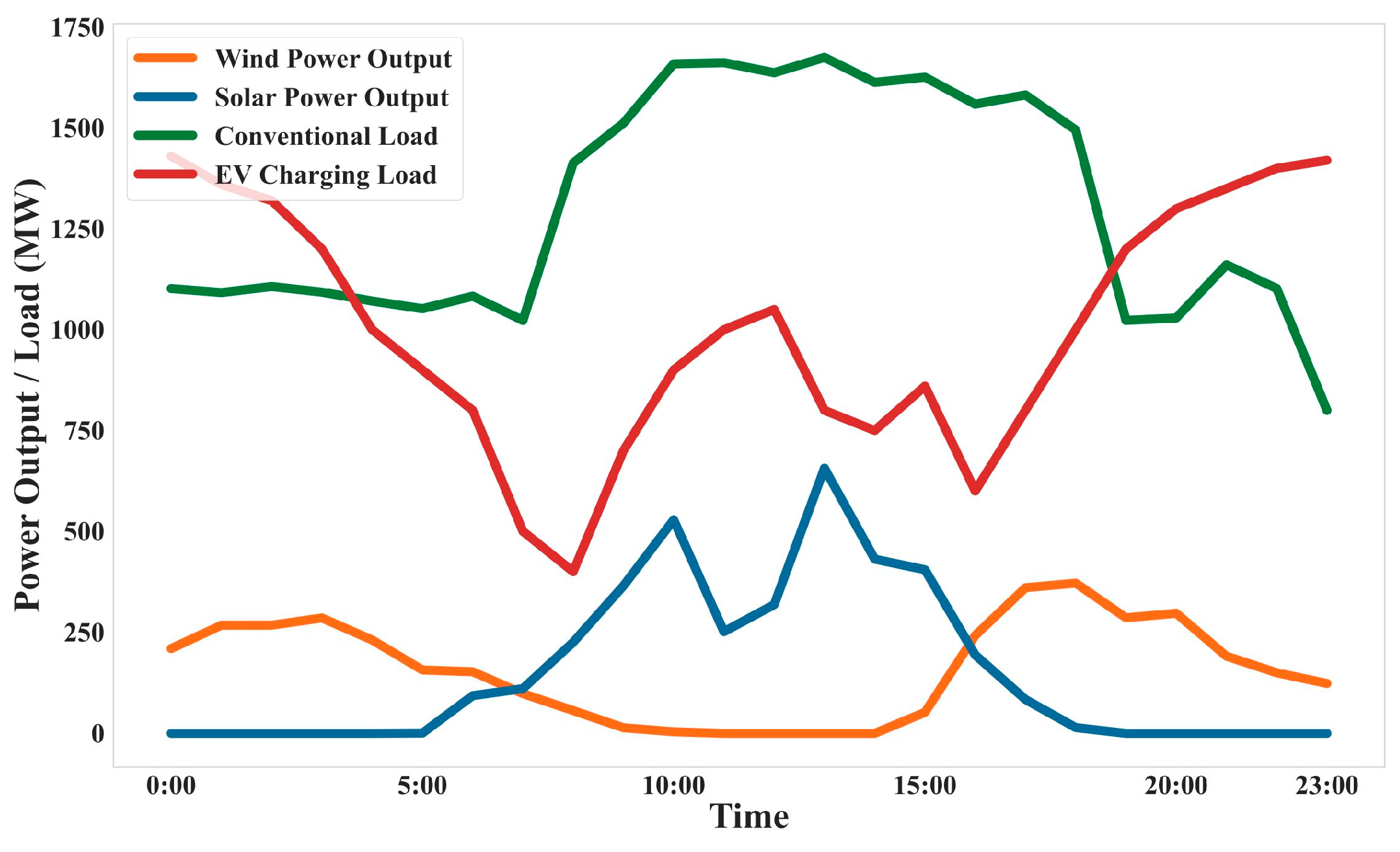
In order to ensure the reliable operation of the regional power system, it is essential to maintain a balance between power supply and demand at each time interval. The system power balance constraint reflects the fundamental requirement that the sum of renewable generation, dispatchable power sources, and EV charging/discharging must match the regional load demand. This relationship is mathematically described as follows:

$$P_{\mathrm{w},t}+P_{\mathrm{G},t}=P_{\mathrm{load},t}+\sum _j^{J}j P_{j,t}^{\mathrm{ev}}$$

(16)

where $P_{\mathrm{G},t}$ is the total output of hydropower units in the region; $P_{\mathrm{load},t}$ is the conventional load forecast in the region; and $J$ is the number of EV charging stations in the region.

3.1.2. Wind Power Output Constraints

Wind power output is inherently variable and largely dependent on real-time meteorological conditions, particularly wind speed. To accurately reflect the generation capabilities of wind turbines, a set of constraints is introduced to model the relationship between wind speed, turbine efficiency, and power output. These constraints ensure that the wind power output remains within feasible operating limits and accounts for the nonlinear characteristics of wind turbine performance. The detailed formulation is given below:

$$0\le P_{\mathrm{w},t}\le P_{\mathrm{w}-\mathrm{m}\mathrm{a}\mathrm{x},t}$$

(17)

$$P_{\mathrm{w},t}={\eta }_t\cdot P_{\mathrm{w}-\mathrm{m}\mathrm{a}\mathrm{x},t}\cdot WindEfficiency\left(v_t\right)$$

(18)

$$WindEfficiency\left(v_t\right)=\left\{\begin{array}{ll}0& \mathrm{if} {\mathrm{v}}_{\mathrm{t}}<{\mathrm{v}}_{\mathrm{cut}-\mathrm{in}}\\ {\displaystyle \frac{{\mathrm{v}}_{\mathrm{t}}-{\mathrm{v}}_{\mathrm{cut}-\mathrm{in}}}{{\mathrm{v}}_{\mathrm{rated}}-{\mathrm{v}}_{\mathrm{cut}-\mathrm{in}}}}& \mathrm{if} {\mathrm{v}}_{\mathrm{cut}-\mathrm{in}}\le {\mathrm{v}}_{\mathrm{t}}<{\mathrm{v}}_{\mathrm{rated}}\\ 1& \mathrm{if} {\mathrm{v}}_{\mathrm{rated}}\le {\mathrm{v}}_{\mathrm{t}}<{\mathrm{v}}_{\mathrm{cut}-\mathrm{out}}\\ 0& \mathrm{if} {\mathrm{v}}_{\mathrm{t}}\ge {\mathrm{v}}_{\mathrm{cut}-\mathrm{out}}\end{array}\right.$$

(19)

$$P_{\mathrm{w}-\mathrm{m}\mathrm{a}\mathrm{x},t}=P_{\mathrm{w}-\mathrm{m}\mathrm{a}\mathrm{x}}\cdot \mathit{CapacityFactor}\left(t\right)$$

(20)

where $P_{\mathrm{w},t}$ is the wind power output at time $t$ and $P_{\mathrm{w}-\mathrm{m}\mathrm{a}\mathrm{x},t}$ is the maximum wind power output. $\mathit{WindEfficiency}\left(v_t\right)$ is a piecewise function that represents the effect of wind speed $v_t$ on the wind power output.

3.1.3. Photovoltaic Power Output Constraints

Photovoltaic power generation is influenced by solar irradiance, temperature, and panel efficiency, leading to time-varying output profiles. To model the operational limits of PV systems, constraints are imposed to ensure that the actual PV output does not exceed its theoretical maximum under given environmental conditions:

$$0\le P_{PV,t}\le P_{PV-\mathrm{m}\mathrm{a}\mathrm{x},t}$$

(21)

where $P_{PV,t}$ is the photovoltaic output at time $t$, and $P_{PV-\mathrm{m}\mathrm{a}\mathrm{x},t}$ is the maximum photovoltaic output.

3.1.4. Total Hydropower Output and Climbing Constraints

Hydropower units play a crucial role in balancing power supply due to their high flexibility and fast response characteristics. However, their operation is still subject to physical and environmental limitations, such as maximum and minimum output levels, as well as ramping constraints that restrict how quickly output can increase or decrease over time. The following equations define these operational boundaries to ensure safe and realistic dispatch of hydropower resources:

$$P_{\mathrm{G},\min }\le P_{\mathrm{G},t}\le P_{\mathrm{G},\max }$$

(22)

$$P_{\mathrm{G},t}-P_{\mathrm{G},t-1}\le R_{\mathrm{G},\mathrm{up}}$$

(23)

$$P_{\mathrm{G},t-1}-P_{\mathrm{G},t}\le R_{\mathrm{G},\mathrm{down}}$$

(24)

where $P_{\mathrm{G},\max }$ and $P_{\mathrm{G},\min }$ are the upper and lower limits of the total hydropower output, and $R_{\mathrm{G},\mathrm{up}}$ and $R_{\mathrm{G},\mathrm{down}}$ are the ramp-up and ramp-down rates of the total hydropower output.

3.1.5. Positive and Negative Spinning Reserve Constraints

To maintain the reliability and stability of the power system in the face of renewable generation uncertainties and load fluctuations, spinning reserve requirements must be considered. These reserves ensure that sufficient upward or downward capacity is available to respond to real-time deviations from forecasts. The following constraints define the minimum positive and negative spinning reserves that hydropower units must provide, based on the forecasted loads and renewable generation levels:

$$P_{\mathrm{G},\max }-P_{\mathrm{G},t}\ge {\alpha }_{\mathrm{load}}{P}_{\mathrm{load},t}+{\alpha }_{\mathrm{w}}{P}_{\mathrm{w},t}$$

(25)

$$P_{\mathrm{G},t}-P_{\mathrm{G},\min }\ge {\alpha }_{\mathrm{load}}{P}_{\mathrm{load},t}+{\alpha }_{\mathrm{w}}{P}_{\mathrm{w},t}$$

(26)

where $P_{PV,t}$ is the photovoltaic output at time $t$, and $P_{PV-\mathrm{m}\mathrm{a}\mathrm{x},t}$ is the maximum photovoltaic output. ${\alpha }_{\mathrm{load}}$ and ${\alpha }_{\mathrm{w}}$ are the spinning reserve coefficients for the wind power and photovoltaic power forecast.

3.1.6. Hydropower Station Water Balance Constraints

The actual operation and regulation characteristics of the hydropower station are taken into account [46].

$$V_{i,t}=V_{i,t-1}-\left[Q_{i,t}+S_{i,t}-I_{i,t}-\sum ^{U_{Pi}}\left(Q_{j,t-d_{j,i}}+S_{j,t-d_{j,i}}\right)\right]\cdot \mathsf{\Delta }t$$

(27)

where $V_{i,t}$ is the final storage capacity, $Q_{i,t}$, $S_{i,t}$ and $I_{i,t}$ are the power generation flow, abandoned water flow and inflow flow, $U{P}_i$ is the hydropower stations that have a direct hydraulic connection with the station $i$, and $d_{j,i}$ is the water flow time lag from upstream station $j$ to downstream station $i$.

3.1.7. Hydropower Reservoir Capacity Constraints

The water storage level of each hydropower station must remain within its operational limits to ensure safe and efficient operation. This constraint is defined as follows:

$$V_i^{\mathrm{m}\mathrm{i}\mathrm{n}}\le V_{i,t}\le V_i^{\mathrm{m}\mathrm{a}\mathrm{x}}$$

(28)

where $V_i^{\mathrm{m}\mathrm{i}\mathrm{n}}$ and $V_i^{\mathrm{m}\mathrm{a}\mathrm{x}}$ are the minimum and maximum storage capacities allowed by hydropower station $i$.

3.1.8. Hydropower Shipping and Irrigation Constraints

In addition to power generation, hydropower stations must meet water demand for shipping and irrigation. The total discharge must therefore stay within specified limits, as shown below:

$$R_i^{\mathrm{m}\mathrm{i}\mathrm{n}}\le Q_{i,t}+S_{i,t}\le R_i^{\mathrm{m}\mathrm{a}\mathrm{x}}$$

(29)

where $R_i^{\mathrm{m}\mathrm{i}\mathrm{n}}$ and $R_i^{\mathrm{m}\mathrm{a}\mathrm{x}}$ are the minimum and maximum discharge flows of hydropower station $i$, respectively.

3.1.9. Hydropower Maintenance Constraints

To account for maintenance schedules and operational conditions, the output of each hydropower station is constrained within allowable maintenance limits, as follows:

$$N_i^{\mathrm{m}\mathrm{i}\mathrm{n}}\le N_{i,t}\le N_i^{\mathrm{m}\mathrm{a}\mathrm{x}}$$

(30)

where $N_i^{\mathrm{m}\mathrm{i}\mathrm{n}}$ and $N_i^{\mathrm{m}\mathrm{a}\mathrm{x}}$ are the minimum and maximum outputs allowed by hydropower station $i$, respectively.

3.1.10. The Current Storage Capacity and the Storage Capacity Control Constraints

To ensure long-term water resource planning and operational continuity, the reservoir storage levels must meet predefined targets at the start and end of the dispatch period. The constraint is expressed as follows:

$$\left\{\begin{array}{l}{V}_{i,0}=V_i^{\mathrm{init}}\\ V_{i,T}=V_i^{\mathrm{fin}}\end{array}\right.$$

(31)

where $V_i^{\mathrm{init}}$ and $V_i^{\mathrm{fin}}$ are the control storage capacities at the beginning and end of the dispatching period of hydropower station $i$.

3.1.11. Hydropower Output Limit Area Constraints

The formula used to determine the power station output limit area constraints in the unit vibration area is shown as follows:

$$N_{i,t}\notin N_i^{limit}$$

(32)

$${\mathcal{N}}_i^{\mathrm{limit}}=[{\underset{\_}{N}}_i^{\mathrm{vib}},{\overline{N}}_i^{\mathrm{vib}}]$$

(33)

where $N_i^{limit}$ is the set of output limit ranges for hydropower station $i$; ${\underset{\_}{N}}_i^{\mathrm{vib}}$ is the minimum allowable output (lower limit) of the $i$-th unit when it enters the vibration zone; and ${\overline{N}}_i^{\mathrm{vib}}$ is the maximum allowable output (upper limit) of the $i$-th unit when it leaves the vibration zone.

3.2. Lower Layer Optimization Model

The lower model mainly optimizes the peak load regulation of each hydropower unit from the perspective of the system’s operation cost, based on the output results of the upper model when maximizing the consumption of wind power and photovoltaic power, taking into account the cost of the deep peak load regulation of hydropower units, and considering the minimum system operation cost as the goal.

3.2.1. Cost Model of Deep Peak Regulation of Hydropower Units

The cost of providing peak load regulation services mainly includes the fixed costs, which mainly include the mechanical losses caused by the unit’s participation in peak load regulation and the costs of various behaviors required during the unit’s peak load regulation process, and the opportunity costs, which refer to the profit loss caused by the unit’s reduced power generation due to its peak load regulation services.

The peak-shaving cost of thermal power units is relatively clear [47]. Through actual research on hydropower stations [48], the fixed cost of peak shaving in hydropower units is mainly the mechanical loss caused by frequent output adjustment in the peak-shaving process.

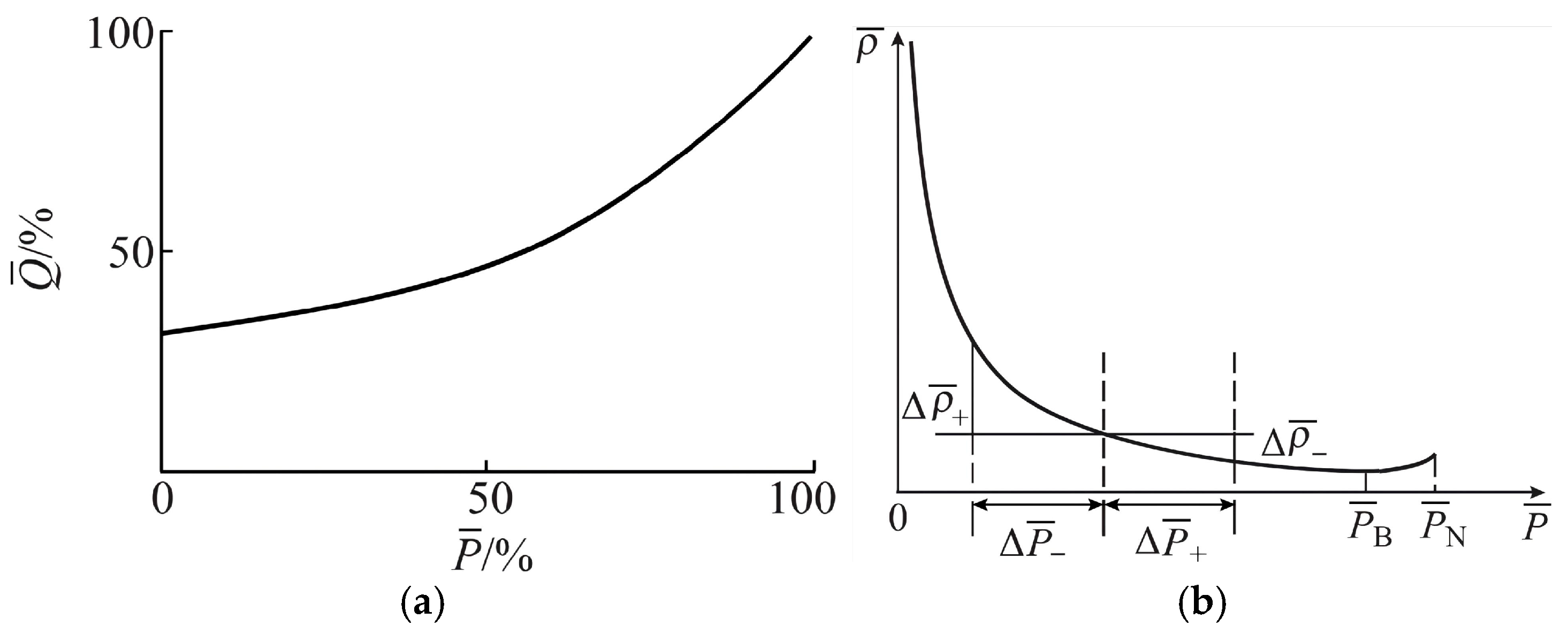
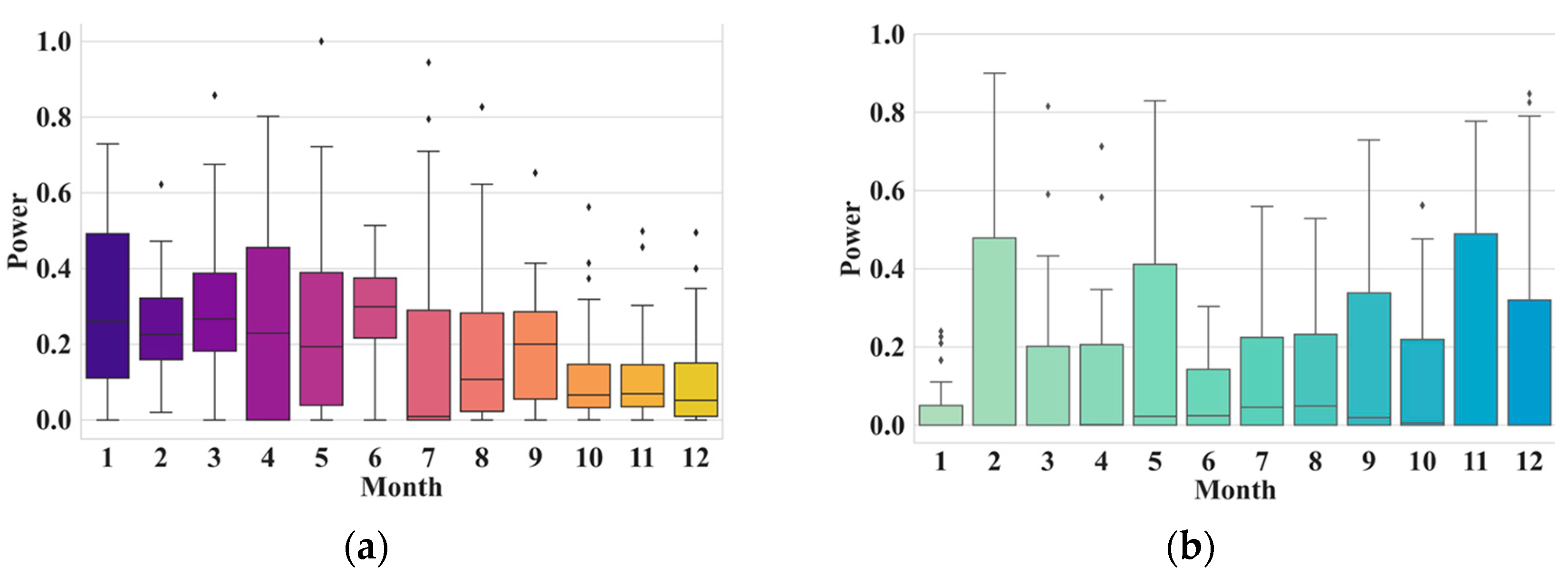
The relative output $\overline{P}$ is the ratio of the actual output $P$ of the unit to the rated output $P_N$ of the unit, and the relative flow $\overline{Q}$ is the ratio of the actual flow $Q$ to the maximum flow $Q_{\mathrm{m}\mathrm{a}\mathrm{x}}$, as shown in Figure 3a [49].

The water consumption rate $\rho =Q/P$ is an important parameter used to characterize the efficiency of a hydropower unit. The relative value of the water consumption rate $\overline{\rho }$ is the ratio of the actual water consumption rate $\rho$ to the minimum water consumption rate ${\rho }_{\mathrm{m}\mathrm{i}\mathrm{n}}$, as shown in Figure 3b [49].

The process used to calculate the peak load compensation for hydropower units is listed below:

(1)

Integrate the gap of $P\left(t\right)<P_{\mathrm{AVE}}-\alpha P_{\mathrm{N}}$ and obtain the corresponding peak load $W$.

(2)

Based on the water consumption rate $\rho$, the peak load $W$ is converted into the water consumption $V$ under the rated water head using the following formula:

$$V=\int \rho \left(P\right(t\left)\right)\left[\right(P_{\mathrm{AVE}}-\alpha P_{\mathrm{N}})-P(t\left)\right]\mathrm{d}t$$

(34)

(3)

Using the water consumption rate ${\rho }_0$ corresponding to the output of the basic peak load limit $P_{\mathrm{AVE}}-\alpha P_{\mathrm{N}}$, $V$ is converted into the minimum power generation $W_0$ using the following formula when no downward peak load regulation is performed:

$$W_0=V/{\rho }_0$$

(35)

Assuming that the unit power generation revenue of the hydropower unit is $p_{\mathrm{w}}$, the compensation fee is $S_c$:

$$S_c=p_{\mathrm{w}}(W_0-W)$$

(36)

Combining Equations (32) and (33), we can obtain the following:

$$S_c=p_{\mathrm{w}}W\left({\displaystyle \frac{\rho }{{\rho }_0}}-1\right)$$

(37)

3.2.2. The Objective Function of the Lower Model

The lower model optimizes the peak load structure of each hydropower unit based on the minimum power abandonment of the upper model, according to the optimized wind power and photovoltaic power consumption, load power of the EV charging station, and total hydropower output. The goal is to maximize the profitability of system operation:

$$\max (\sum _{t=1}^{T}t=\sum _{i=1}^{N}i=W_{load}\cdot P_1+W_{EV}\cdot P_2+S_c-S_{i,t}^G-S_{i,t}^{\mathrm{PV}}-S_{i,t}^W-S_{i,t}^{\mathrm{deploy}})$$

(38)

where $W_{load}$ is the conventional load power consumption, $P_1$ is the conventional load electricity price, $W_{EV}$ is the electric vehicle charging amount, $P_2$ is the electric vehicle charging price, $S_c$ is the compensation amount, $S_{i,t}^{\mathrm{G}}$ is the cost of power generation for the hydropower station, $S_{i,t}^{\mathrm{PV}}$ is the cost of photovoltaic power generation, $S_{i,t}^W$ is the cost of wind power generation, and $S_{i,t}^{\mathrm{deploy}}$ is the total dispatch cost of the system.

3.3. Model Solving

The upper and lower layers of the hierarchical optimization model established in this paper belong to mixed-integer nonlinear programming problems. In order to reduce computational complexity, linearization processing is required. Equations (14)–(30) in the upper model and Equations (34)–(38) in the lower model are both linearized piecewise. Finally, taking an actual regional system containing a large number of EV charging stations and hydropower stations as an example, a deep reinforcement learning (DRL) algorithm is used to solve and analyze the problem, thereby calculating the maximum operating profit and various parameters to verify the effectiveness of the proposed scheme.

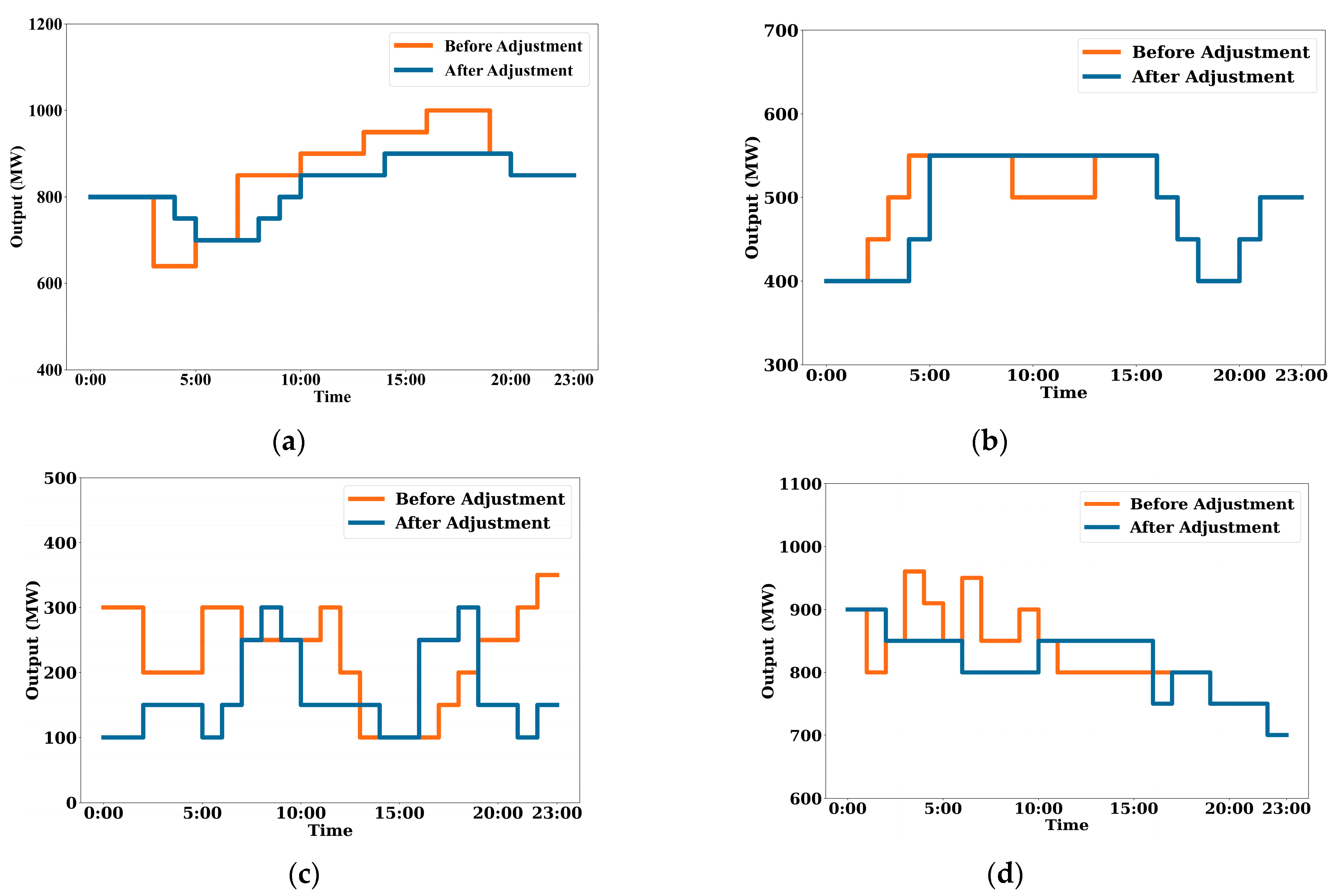
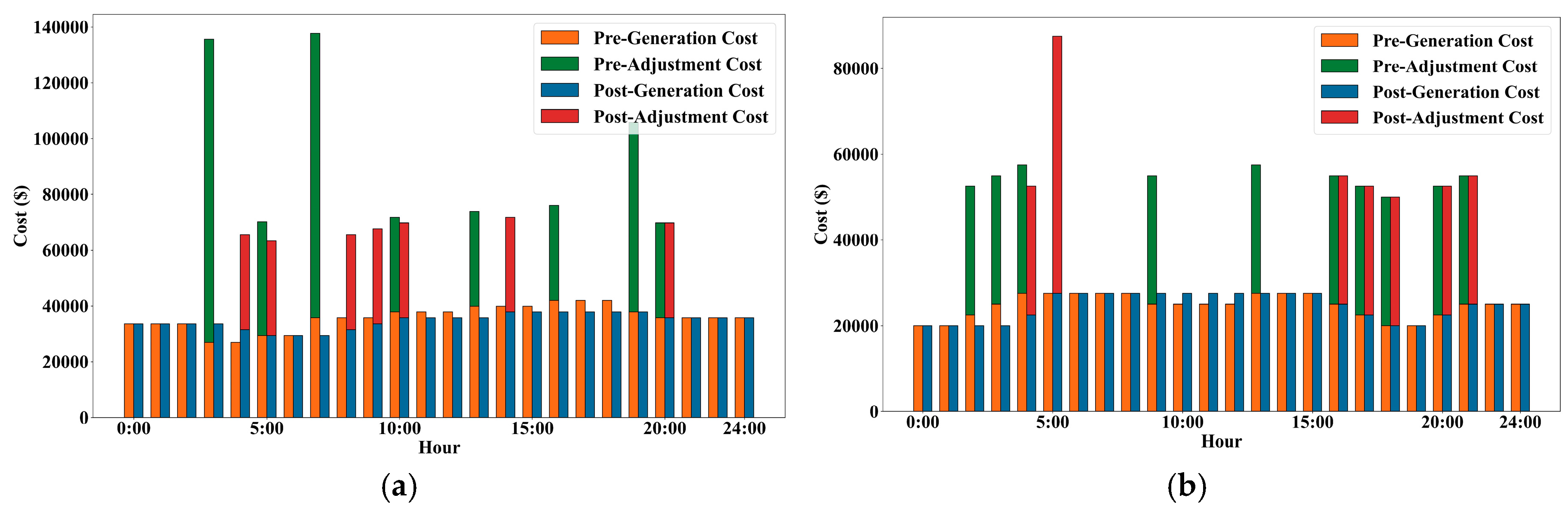
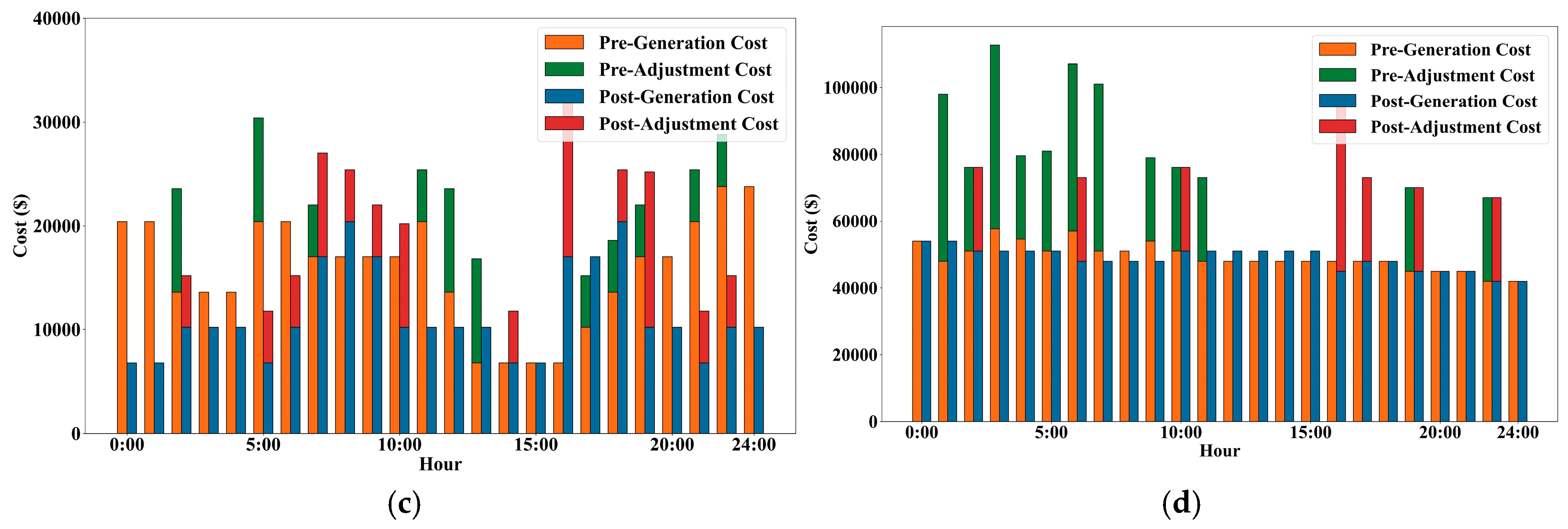
In actual operation, in order to balance economy and the dispatch flexibility, we stipulate that the hydropower station receives a power dispatch instruction from the power grid once an hour and that each power adjustment is made in multiples of 50 MW.

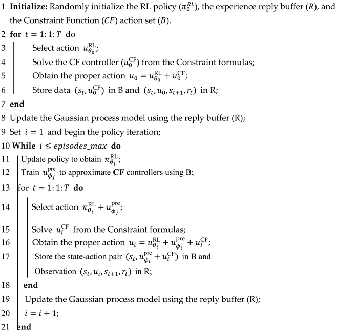
In order to ensure the strict implementation of the constraint listed above and thus ensure the safety of the adjustment process, we organize the formulas listed above into a constraint function (CF) and control it in combination with the input in the deep reinforcement learning algorithm [50]. The training algorithm of the DRL-CF network is summarized as follows.

The examined DRL-CF control method was implemented in Python (version 3.7) through PyTorch (version 2.0). The training processes were executed on a Windows system with an AMD Ryzen 7 7840HS with Radeon 780M Graphics 3.80 GHz and 32 GB of RAM. The hardware was sourced from AMD, CA, USA. The actor and critic networks included two hidden layers, with 256 hidden units, which were trained using the Adam optimizer. The tanh activation was adopted for the output layer. Other system input parameters of the RL agent are summarized in

Table 1. Parameter settings of the test system.

Symbol	Description	Value
${\beta }_1,{\beta }_2$	Weight factors	5800
$\kappa$	confidence probability	3
$\eta$	Safe coefficient	0.95
$\gamma$	Discount factor	0.9
$\left|\mathcal{K}\right|$	Mini-batch sampled data	300
${\delta }_{{\theta }^Q}$	$\mathrm{Learning} \mathrm{rate} \mathrm{of} \mathrm{critic} \mathrm{network} Q_{\pi }$	0.001
${\delta }_{{\theta }^{\pi }}$	Learning rate of actor-network π	0.0001

.The DRL-CF algorithm is shown as Algorithm 1.

Algorithm 1: DRL-CF algorithm

4. Case Study

4.1. Case Description

This study uses a real urban regional power grid in Sichuan, China, to verify the effectiveness of the established model. The regional power grid has three key features: (1) rich hydropower resources and a large hydropower installed capacity; (2) good new energy endowment, with a high wind power and photovoltaic installed capacity; (3) a relatively high proportion of electric vehicle load in the urban area among the total regional load. Since hydropower is a clean energy, it faces problems related to water abandonment restrictions and the limited capacity of system regulation support. Obviously, due to the high proportion of new energy access, the regional power grid relies heavily on peak-shaving resources, and peak-shaving resources need to be further explored. The load and installed power capacity scale in this regional power grid are shown in

Table 2. Installed capacity of the power generation and charging stations (MW).

Category	Station	Installed Capacity (MW)
Wind Power	Wind Power	2000
Photovoltaic Power	Photovoltaic Power	1000
Hydropower	Hydropower Station A	1200
	Hydropower Station B	600
	Hydropower Station C	400
	Hydropower Station D	1000
EV Charging Stations	Charging Station A	200
	Charging Station B	300
	Charging Station C	400
	Charging Station D	600

. The relevant regulation parameters of the hydropower units and EV charging stations are obtained from an actual survey of the regional power grid.

According to the actual operating constraints of hydropower stations and charging stations, the maximum power adjustment range of different hydropower stations at adjacent times is solved. The specific data are shown in

Table 3. Power change limits for hydropower and charging stations.

	Power Change Between Adjacent Times (%)	Maximum Power Drop (%)
Hydropower Station A	30%	-
Hydropower Station B	25%	-
Hydropower Station C	50%	-
Hydropower Station D	15%	-
Charging Station A	40%	30%
Charging Station B	45%	30%
Charging Station C	30%	30%
Charging Station D	35%	30%

. The cost of power generation in hydropower stations in the region and data regarding the time-of-use electricity price in charging stations are shown in

Table 4. Generation and regulation costs for hydropower stations (per MWh).

Station	Generation Cost (USD/MWh)	Regulation Cost (USD/MWh)
Hydropower Station A	68	420
Hydropower Station B	60	500
Hydropower Station C	50	600
Hydropower Station D	42	680

and

Table 5. Time-of-use tiered pricing for EV charging stations (per MW).

Time Period	23:00 to 07:00	08:00 to 15:00	16:00 to 18:00	19:00 to 22:00
Charging Station Price (USD/MW)	50	80	100	120

[51].

In order to better illustrate the hierarchical optimization strategy that was proposed in this paper to maximize the impact of wind power and photovoltaics, this study selected two comparative schemes for analysis. The two comparative schemes are as follows:

Case 1: EV charging stations do not participate in regulation.

Case 2: EV charging stations participate in coordinated optimization and regulation.

The per unit values, which represent the ratio of actual power generation to the rated installed capacity of wind power and photovoltaic power in the region for 12 months in 2023, were selected; the corresponding box plot was then generated, as shown in Figure 4. We can see that there is a clear relationship between power generation and the month.

As can be seen from the box plot in Figure 4, the photovoltaic output in 2023 showed obvious seasonal characteristics. The peak is concentrated in June–August in summer, and the superposition of sunshine intensity and sunshine duration makes the monthly power generation during this period generally larger. The fluctuation is small in winter, and the boxes in December and January–February are relatively flat, indicating that the overall power generation level is low in winter due to restrictions such as cloud cover and few sunshine hours.

At the same time, the wind power output also shows its own seasonal laws. The fluctuation is the largest in spring and autumn, and the wind speed in March–May and September–November easily changes, with more extreme daily output values; especially in March and November, there are often “peaks” of power generation caused by unconventionally high wind speeds. The power generation is relatively slow in July–August in midsummer and in January–February in late winter.

The typical 24 h power generation and load curve of the power grid in this area are shown in Figure 5. Wind power has a small peak at around 2:00 a.m., is almost at its lowest point in the morning, and rebounds again around 15:00–18:00 in the afternoon before gradually declining; photovoltaic power starts to generate electricity around 6:00, reaches its daytime peak at 10:00–14:00, and then rapidly decays until the end of the evening; conventional load remains at a low level from 0:00 to 6:00, jumps to a high level around 8:00, falls back in the evening, and continues to decrease at night; the electric vehicle charging load is also high from 0:00 to 2:00, and then drops to the lowest point at 6:00, with a small rebound in the afternoon, a main peak from 18:00 to 23:00 in the evening, and gentle fluctuations around 23:00.

4.2. Results Analysis

4.2.1. Analysis of DRL and MILP

This paper uses the MILP method as a control. Based on the existing two-layer model, the commercial solver Gurobi is used to directly solve the linearized MILP. The result of MILP is considered very close to the “optimal” solution in the true sense and can be regarded as an upper limit reference. The comparison results are shown in

Table 6. Analysis of DRL and MILP.

Method	Generation (MWh)	Generation Cost (USD)	Adjustment Cost (USD)	Calculation Time (min)
DRL	55,100	2,863,600	773,000	2.3
MILP	53,230	2,832,900	752,000	6.7

. Although MILP has a lower generation cost, it takes too long and is difficult to apply online in complex systems with the joint dispatch of multiple power stations. DRL is significantly better than MILP in real time and in terms of flexibility. Although its cost is slightly higher, its rapid response capability and long-term cost optimization potential make it more suitable for the online dispatching of power grids with a high proportion of new energy. MILP can be used as an offline benchmark verification tool.

4.2.2. Analysis of Social Total Peak Shaving Effect

A comparison of the total peak load regulation effect indicators of the system under different schemes is shown in

Table 7. Total peak load regulation effect of different schemes.

Case	Generation (MWh)	Generation Cost (USD)	Adjustment Cost (USD)	Curtailed (MWh)	Curtailment Rate (%)
Case 1	57,600	3,013,260	1,240,600	9883	17.1%
Case 2	55,100	2,863,600	773,000	5012	9.09%

. In terms of the overall economic efficiency of the system, compared with Case 1, Case 2 effectively improves the economic efficiency of the system peak load regulation, reducing the water and electricity costs by 4.34% and the system operation costs by 5.67%.

The results show the effect before and after adjustment from the perspective of several key indicators. The change in power generation shows a reduction in power generation, which shows that the cost of power generation has been reduced. Through adjustment, the cost of power generation is reduced by nearly USD 150,000, showing that under optimized dispatch, the system can operate at a lower cost, reducing excess in order to regulate resource consumption. Curtailment was reduced by about half, indicating that the regulated system made better use of renewable energy and reduced energy waste.

Combined with Table 6 and Figure 6, it can be seen that Case 2 significantly reduced the amount of power abandoned in the system, which was mainly concentrated in the period of 03:00–09:00, reducing the total power abandonment rate by 46.8%. Figure 5 is a histogram of the overall system output and wind abandonment under different schemes. In order to cope with the consumption of wind power and photovoltaic power, the output adjustment of hydropower units is more frequent in Case 1, while in Case 2, due to the participation of EV charging stations in the adjustment, the number of hydropower unit output adjustments is significantly reduced, and the total hydropower generation required to meet the load is reduced. The amount of abandoned power fluctuated greatly before the adjustment; the peak in abandoned power around 7:00 in the morning was particularly obvious, and this was related to the fact that the hydropower station increased power in advance in order to increase the morning peak load. After the adjustment, the amount of abandoned power was more stable and balanced. The adjustment of the charging stations reduced the peak in abandoned power in the morning, making the overall utilization rate for wind power and photovoltaic power higher, and avoiding the increase in abandoned power due to large load fluctuations. In terms of the overall effect, the adjusted solution significantly optimizes the operating effect of the system.

Figure 7 compares the system’s overall output and abandoned power under different schemes, Figure 7a shows the situations when EV charging station is not involved in the regulation, and Figure 7b shows the situation when the EV charging station participates in the regulation.

The specific changes are summarized as follows:

(1)

Load reduction during morning and evening peaks: The regulation of EV charging stations helps to flatten the peak electricity consumption in the morning and evening, avoiding excessive power generation demand during peak hours.

(2)

Improved utilization of photovoltaic power generation. The peak fluctuation in new energy is effectively flattened, reducing the waste of photovoltaic power generation.

(3)

Load smoothing. The overall system load curve after the participation of EV charging stations during regulation is smoother, indicating that the regulation of electric vehicles makes the system’s fluctuations smaller and improves the stability and efficiency of the power system.

4.2.3. Analysis of Hydropower Output

Hydropower station C has the largest power adjustment range at adjacent moments and has good flexibility, and because of its small installed capacity, its adjustment cost is the lowest. It is determined to be the main peak-shaving power station, with the other three hydropower stations being auxiliary peak-shaving power stations. As shown in Figure 8, after the adjustment, the hydropower output was relatively stable. The fluctuation observed in the hydropower stations in Figure 8a,b,d is significantly weakened. This shows that the participation of EV charging stations can make the regulation of hydropower output smoother, reduce large fluctuations, reduce the burden of hydropower generation to a certain extent, and reduce the overall generation of hydropower.

4.2.4. Analysis of EV Charging Station Revenue

The revenue of a 24 h EV charging station under the tiered electricity price is shown in Figure 9, which shows that from 3:00 to 8:00, the load growth rate is slower than the growth of total power generation. At this time, the EV charging station consumes more electricity, thereby obtaining more revenue. However, since this is the lowest point of the ladder electricity price, the difference in revenue during this period is not obvious. From 15:00 to 17:00, due to the increase in the ladder electricity price at this time, the revenue changes significantly. From 18:00 to 20:00, since this is the peak period of power demand, charging stations cannot make larger-scale adjustments. Therefore, the revenue before and after the adjustment is basically the same, and since the ladder electricity price is the highest, the revenue is also the highest at this time. Overall, the revenue of electric vehicles before and after the adjustment increased from USD 1,883,300 to USD 2,026,000, an increase of 7.58%, and a certain income growth was achieved.

4.2.5. Analysis of Hydropower Station Cost

The cost of a hydropower station consists of two parts: the cost of power generation and the regulation cost. Below is a cost analysis of the four hydropower stations when they are running 24 h a day. The Figure 10 shows that compared with before regulation, the power generation costs of the four hydropower stations all decreased after regulation; Figure 10c shows that the power generation cost of hydropower station C decreased significantly, with a larger decrease from 0:00 to 3:00. Compared with before regulation, Figure 10a,d shows that the regulation costs of hydropower stations A and D decreased significantly, indicating that after electric vehicles participated in the regulation, the peak regulation times and peak regulation amplitudes of the four hydropower stations were significantly reduced, which played a role in stabilizing the power generation of the hydropower stations and absorbing wind power and photovoltaic new energy.

4.2.6. Sensitivity Analysis of Key Parameters on Model Performance

To verify the robustness and adaptability of the proposed model, this paper conducts sensitivity analysis on the following three key parameters:

(1)

Electricity price fluctuation (time-of-use electricity price at charging stations)

(2)

Electric vehicle charging station capacity $P_{\mathrm{ev},\max }$

(3)

Hydropower ramp limit $R_{G,\mathrm{up}}/R_{G,\mathrm{down}}$

As shown in Figure 11, high electricity prices suppress peak charging and optimize the load distribution, meaning that users switch to valley charging, resulting in an increase in abandoned electricity.

When adjusting the charging capacity, an increase in capacity enhances regulation capabilities and significantly reduces costs; an insufficient capacity leads to abandoned electricity and a surge in costs.

When adjusting hydropower slope restrictions, an increase in slope rate can enable the flexible regulation of hydropower and promote the consumption of new energy; the rigid restriction of a reduced slope rate exacerbates abandoned electricity and regulation costs.

5. Conclusions

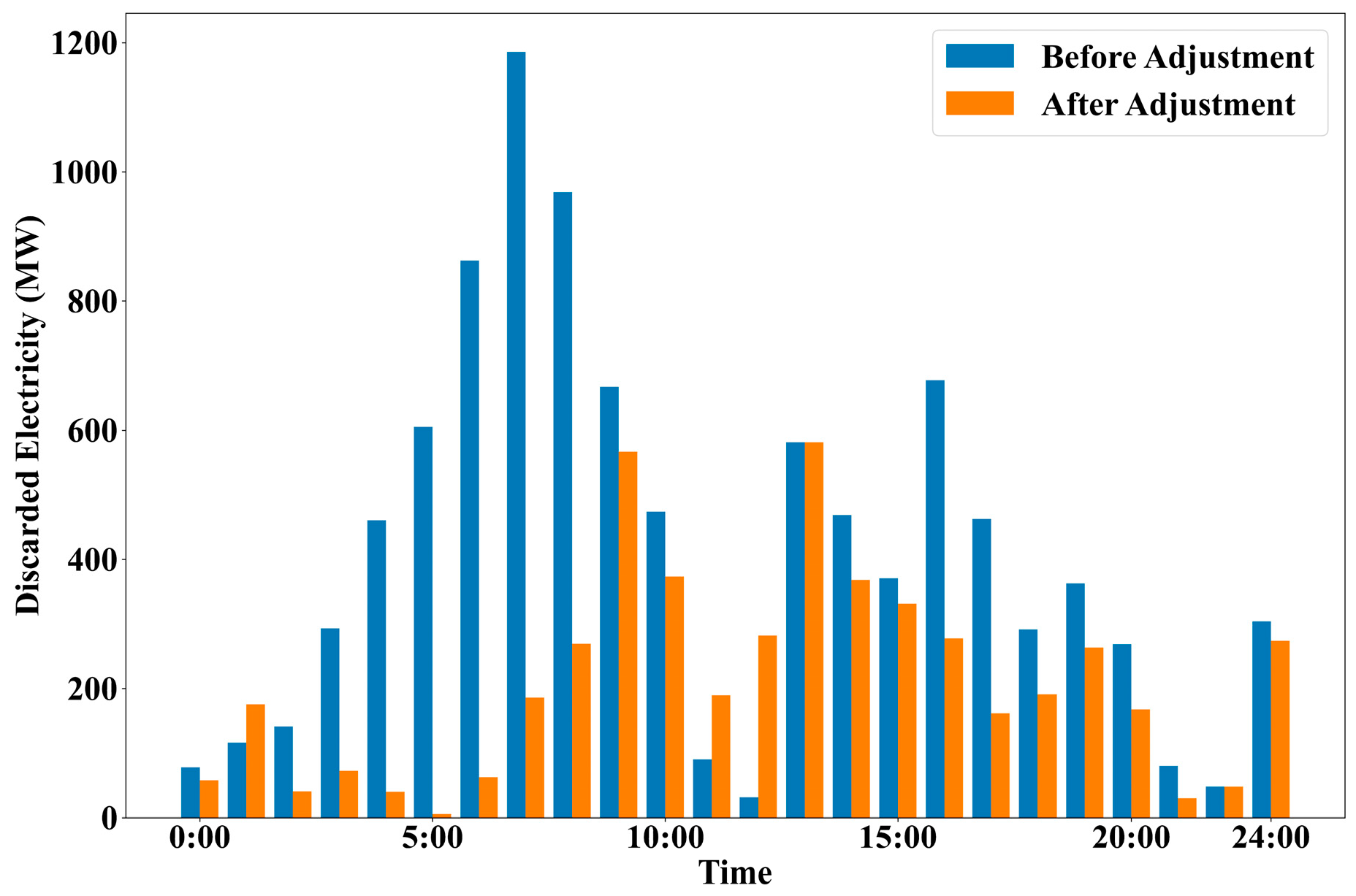
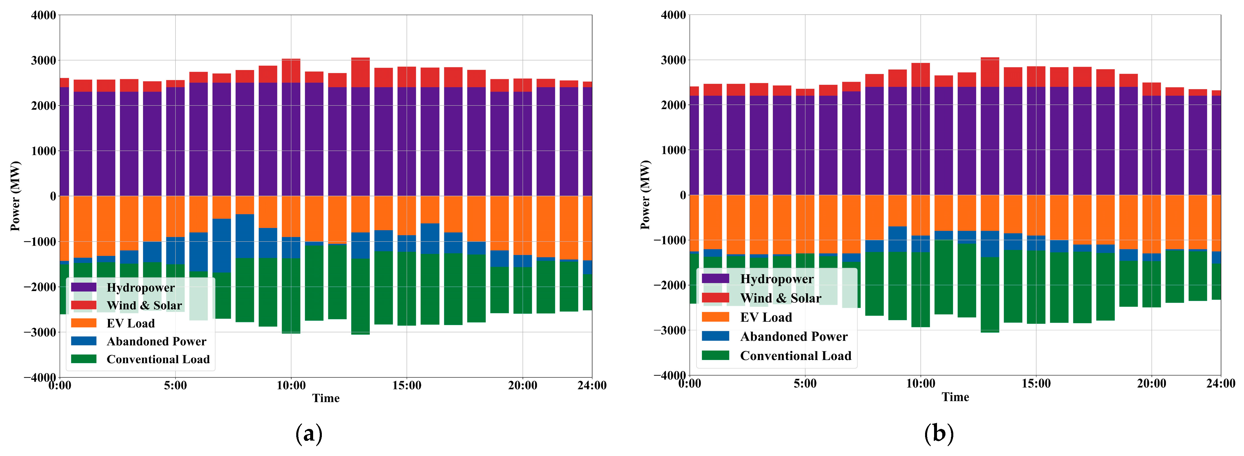
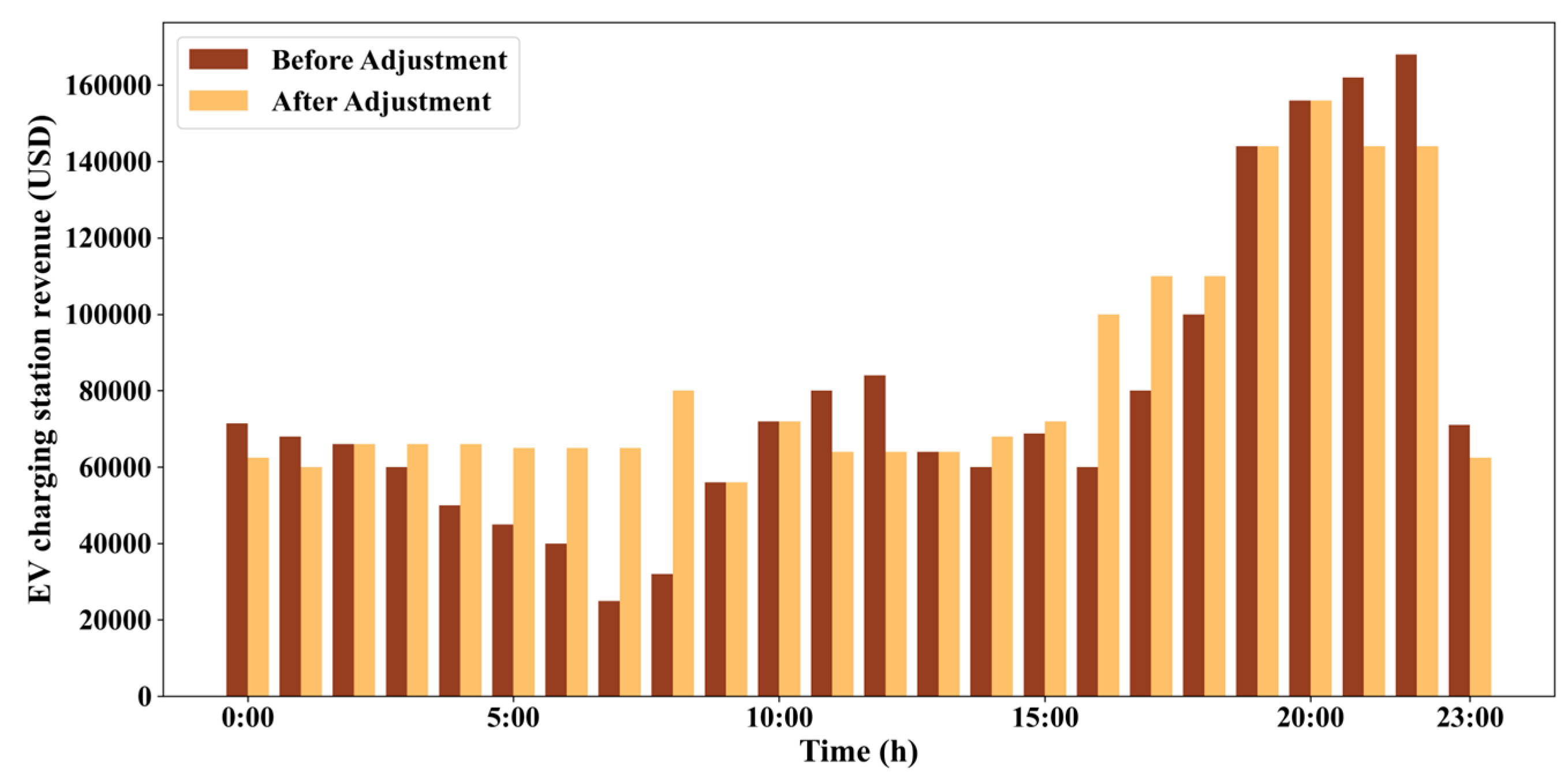
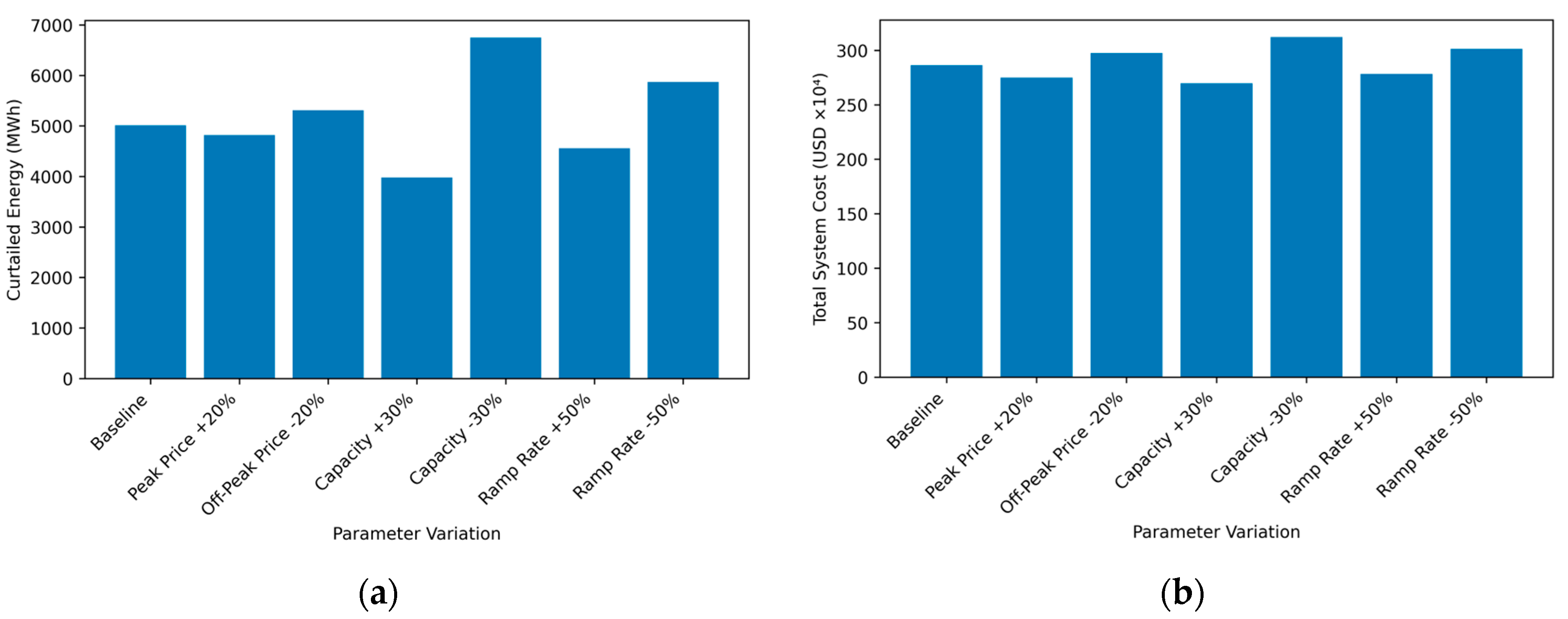
This paper considers incorporating the load of EV charging stations into the optimal dispatching of the power grid, and jointly participates in the peak-shaving operation of the integrated water–wind–solar system with the deep peak shaving of hydropower units; it also establishes a hierarchical optimization model with the minimum system power abandonment and the minimum operating cost. Finally, taking a real regional system with a high proportion of wind power and photovoltaic power and rich hydropower resources as an example, the effectiveness of the proposed strategy is verified, the economic and technical impact of the deep peak shaving of hydropower units is analyzed, and the following conclusions are obtained:

(1)

The proposed scheme can effectively improve the comprehensive peak-shaving effect of the system, and reduce the cost of hydropower in the regional example system by 4.34% and the system operation costs by 5.67%, respectively; the load regulation of EV charging stations and the hierarchical coordination of deep hydropower regulation promote wind power consumption, which relatively reduces the abandoned wind volume by 46.8%.

(2)

Under the proposed scheme, the economic and technical performance of hydropower units participating in the peak shaving of the power grid is improved. The participation of the load of EV charging stations in grid regulation significantly alleviates the peak-shaving pressure of hydropower units, reduces the regulation of hydropower units and the amount of electricity, optimizes the deep peak-shaving structure of hydropower units, and reduces the cost of hydropower regulation and total hydropower generation, which lowers the cost of generating hydropower.

(3)

The proposed hierarchical optimization model focuses on verifying the support potential and effect of the load of charging stations on the system’s peak shaving in the regional power grid, and has a significant effect on the integrated water–wind–solar regional system with a high proportion of wind power and photovoltaic power and a high proportion of charging stations; this is especially true for the coordination of peak-shaving strategies with hydropower peak-shaving resources, which has great significance for practical guidance.

In the future, the model can be combined with the secondary control of DC microgrids to utilize fast control dynamics to achieve large-scale communication, networked sensor sampling and computing loads [52]. At the same time, decentralized operation methods that avoid risks should be considered to effectively limit the systemic risks existing in the joint system [53]. For the distribution of benefits, the random double-level optimal allocation method can be considered to ensure the distribution of the benefits of different entities in the joint system when electricity prices are uncertain [54].