Aggregation Method and Bidding Strategy for Virtual Power Plants in Energy and Frequency Regulation Markets Using Zonotopes

Abstract

Aggregating and scheduling flexible resources through virtual power plants (VPPs) is a key measure used to improve the flexibility of new power systems. To maximize the regulation potential of flexible resources and achieve the efficient, unified scheduling of flexible resource clusters by VPPs, this study proposed a flexible resource aggregation method for VPPs and a bidding strategy for participation in the electricity and frequency regulation markets. First, considering the differences in the grid frequency regulation demand across periods, an improved zonotope approximation method was adopted to internally approximate the feasible region of flexible resources, thereby achieving the efficient aggregation of feasible regions. On this basis, the aggregation model was applied to the optimization model for VPPs, and a day-ahead double-layer bidding model of VPPs participating in the electricity and frequency regulation markets was proposed. The upper layer optimizes the bidding strategies to maximize the VPP revenue, while the lower layer achieves joint market clearing with the goal of maximizing social welfare. Finally, case studies were undertaken to validate the effectiveness of the proposed method.

1. Introduction

1.1. Background

Driven by dual carbon goals and the construction of new power systems, the penetration rate of renewable energy keeps rising, while the regulatory capacity of traditional power generation resources keeps declining. The pressure on the balance of power supply and demand in the power system is further intensifying, significantly increasing the demand for flexible resources in power systems [1]. The participation of flexible resources in dispatch can remarkably enhance the flexible regulation ability and stability of a power grid [2]. However, these resources have small capacities and large quantities, posing challenges related to their scheduling and management [3]. Through the large-scale aggregation and efficient unified allocation of flexible resources by VPPs, the regulation potential of flexible resources can be fully tapped, which is an effective means for flexible resources to participate in grid regulation. VPPs can contribute to the safe and stable operation of a power system by participating in the electricity market, as well as the frequency regulation and other auxiliary service markets [4,5]. VPPs will become an essential component of future power systems, providing solid support for achieving the goal of green and low-carbon energy transformation.

1.2. Literature Review

In terms of feasible region aggregation for flexible resources, geometric computation methods are typically used to model the operational flexibility regions of devices as polytopes. These methods integrate the flexibility regions of multiple devices through the Minkowski sum, transforming the flexible resource aggregation problem into a geometric computation task. From the perspective of geometric approximation, these methods can be classified into internal and external approximations. External approximation methods [6,7,8] yield feasible regions larger than the actual ones, introducing infeasible solutions that may pose safety risks during actual dispatch. Internal approximation methods ensure that all the solutions within the feasible region are feasible, but they sacrifice accuracy when individual flexibilities vary significantly, resulting in conservative aggregation results. Based on the sequence of approximation and aggregation, geometric methods can also be divided into holistic approximation [9,10,11] and piecewise approximation followed by linear superposition. The former directly approximates the aggregation flexibility region as a whole without considering the form of the feasible region of a single resource, resulting in more sacrifice of the feasible region. The latter, with a higher approximation accuracy, is widely used, but its aggregation precision and computational efficiency vary depending on the chosen approximated feasible region shapes. Using the piecewise internal approximation approach, the authors of [12] employed centrally symmetric zonotopes to internally approximate the feasible region of flexible resources. The authors of [13] used hyper-rectangle models with quadratic terms to approximate the feasible region of demand response models. The authors of [14] established active power-approximation feasible regions and active–reactive power-stochastic-approximation feasible regions for micro-power aggregation flexibility. To address feasible region loss during approximation, the existing geometric methods mostly aim to maximize the overall feasible region across all periods during aggregation, neglecting differences in the grid frequency regulation demand across periods. Consequently, the regulatory potential of flexible resources cannot be fully utilized during periods of high grid frequency regulation demand. Therefore, it is necessary to consider the difference in the regulation demand of different periods when aggregating and allocate more feasible region loss to the period with less grid regulation demand, so as to fully exploit the regulatory capabilities of flexible resources.

Regarding VPP participation in market competition and optimal dispatch, the current research on applying geometric aggregation models of flexible resources to bidding and optimization models is limited. The authors of [15] considered a VPP containing a wind turbine (WT), photovoltaic (PV) cells, energy storage, and flexible loads, studying their participation in peak-shaving ancillary services. The authors of [16] proposed an intelligent peak-shaving pricing strategy for a VPP with air conditioners, electric water heaters, and adjustable loads. These studies directly incorporated the operational models of flexible resources into optimization constraints without aggregating the internal flexible resources beforehand. Thus, further research is needed to apply flexible resource aggregation models to VPP bidding models and explore coordinated interaction modes between VPPs and flexible resource clusters. Based on the influence of market members on the clearing prices, participants can be classified as price makers or price takers. The authors of [17] treated aggregated distributed resources as price takers, considering temporal instability, and proposed an optimal operation strategy for VPP participation in day-ahead and real-time energy markets. The authors of [18] proposed a two-stage optimization strategy for battery-swapping stations participating in energy and frequency regulation markets, with the first stage formulating demand response strategies for electric vehicle clusters and the second stage determining market competition strategies. Since the VPP in this study aggregated a large number of flexible resources with sufficient capacity to influence market-clearing prices, it was necessary to treat the VPP as a price maker and incorporate market clearing into the decision-making model.

1.3. Contributions

By synthesizing the above analysis to fully exploit the regulatory potential of flexible resources and achieve the efficient unified scheduling of flexible resource clusters by VPPs, this study investigated feasible region aggregation and market competition strategies. First, considering the differences in the grid frequency regulation demand across periods, an improved zonotope approximation method was proposed to internally approximate the feasible region of flexible resources, enabling efficient aggregation. Subsequently, the aggregation model was applied to the VPP optimization model, proposing the day-ahead double-layer bidding model for VPP participation in the energy and frequency regulation markets. The upper layer optimizes the bidding strategies to maximize the VPP revenue, while the lower layer achieves market joint clearing to maximize social welfare. Finally, case studies validated the effectiveness of the proposed method.

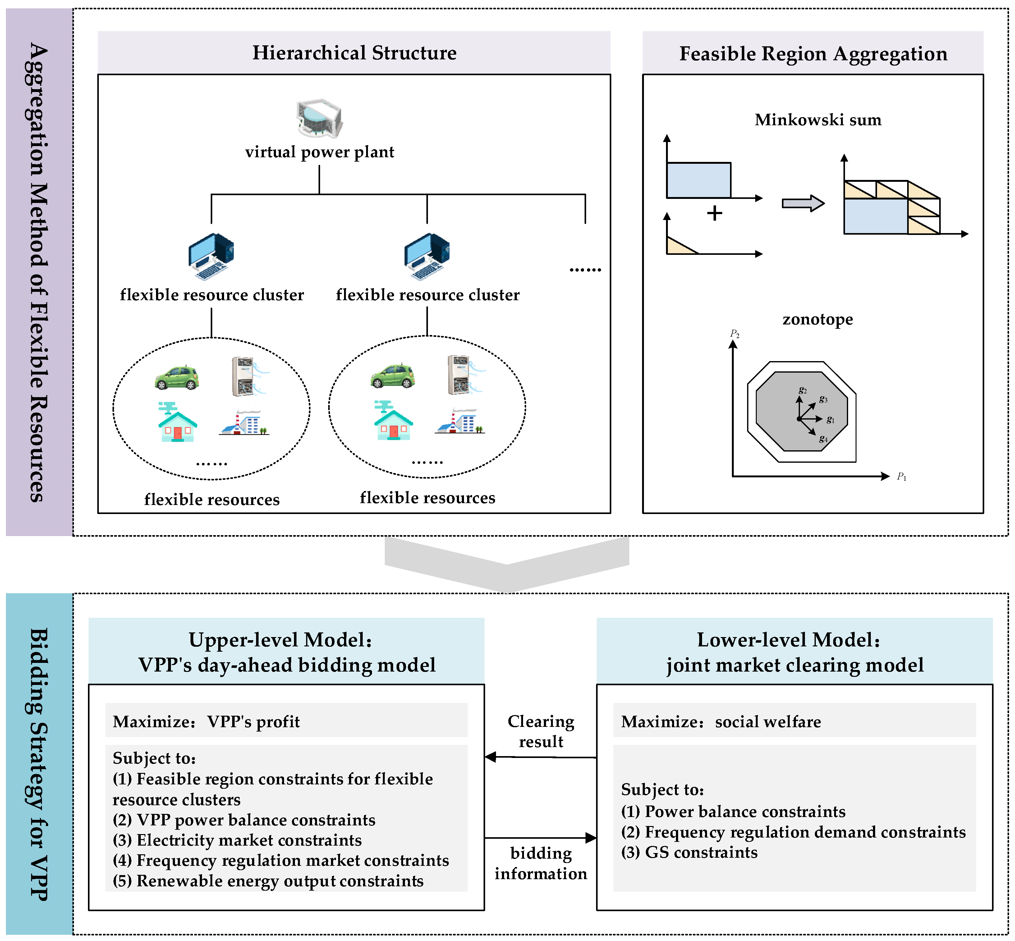
2. Research Methodology

A flowchart of the proposed aggregation method and bidding strategy is shown in Figure 1. This research considered flexible resources and the VPP formed by their aggregation as the research objects and examined the aggregation method of the flexible resources, as well as the bidding strategies of the VPP participating in the energy and frequency regulation markets. A single demand-side flexible resource has a small capacity and cannot reach the threshold of market access. Flexible resources can first be aggregated into several clusters. Section 3 investigates the aggregation method of demand-side flexible resources. After the flexible resources are aggregated, the flexible resource clusters can be efficiently and uniformly dispatched through the VPP. Section 4 examines the bidding strategy of the VPP in the scenario of the VPP participating in the electricity and frequency regulation auxiliary service markets.

3. Aggregation Method of Flexible Resources Based on Zonotope

3.1. Feasible Region of Flexible Resources

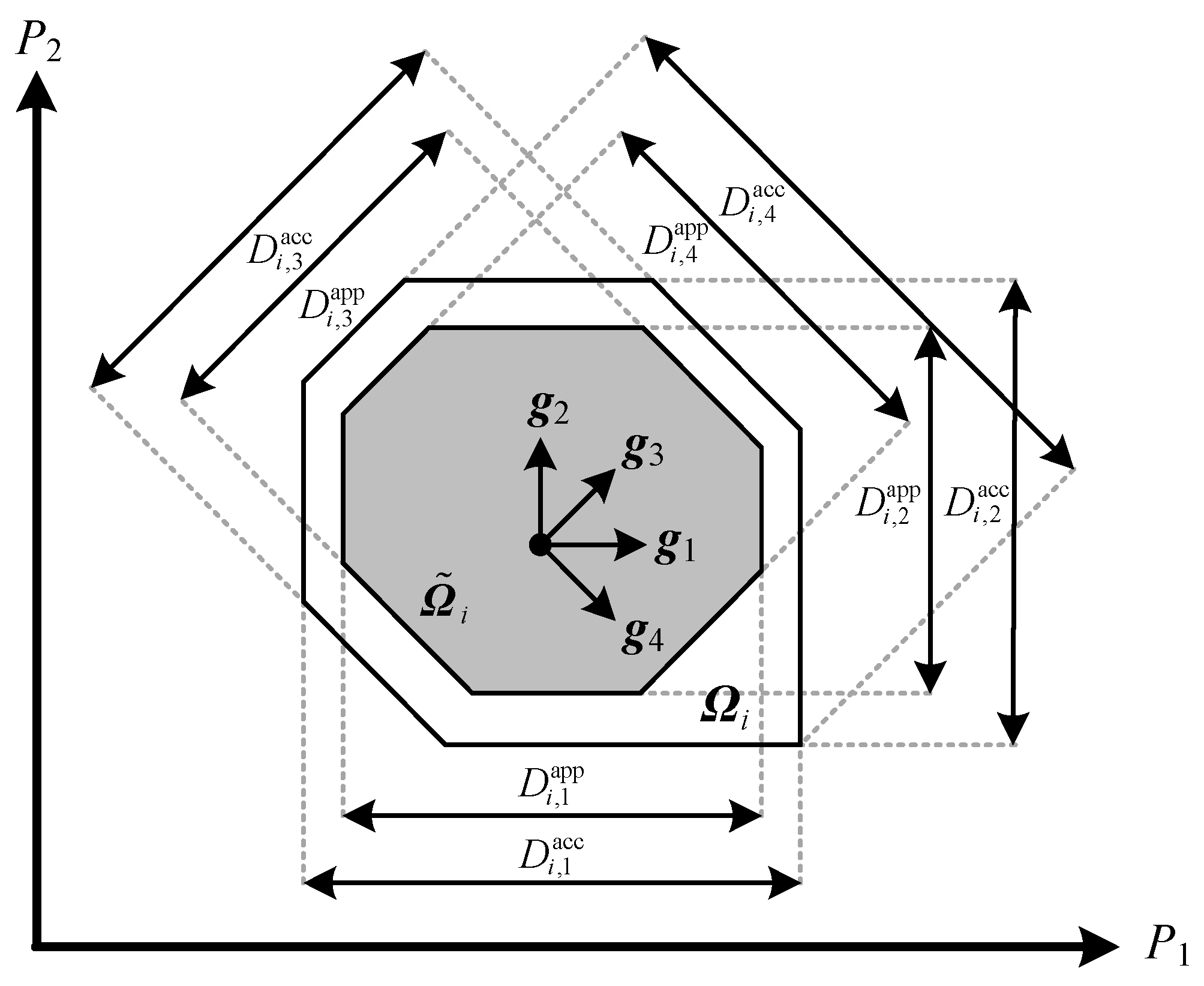
With reference to [19], the operational models of various flexible resources within VPPs can be unified into the following form, where (1) is the power constraint, (2) is the ramp constraint, and (3) and (4) are the energy constraints.

$$P_{i,t}^{\min }\le P_{i,t}\le P_{i,t}^{\max }$$

(1)

$$-{\delta }_i^{\mathrm{d}}\Delta t\le P_{i,t}-P_{i,t-1}\le {\delta }_i^{\mathrm{u}}\Delta t$$

(2)

$$E_{i,t}^{\min }\le E_{i,t}\le E_{i,t}^{\max }$$

(3)

$$E_{i,t}=E_{i,t-1}+{\eta }_i{P}_{i,t}\Delta t+W_{i,t}$$

(4)

where $i=1,2,\dots ,n$, and $n$ is the number of flexible resources; $t=1,2,\dots ,T$, and $T$ is the scheduling horizon; $\Delta t$ is the time interval; $P_{i,t}$ is the power of flexible resource $i$ during period $t$; $P_{i,t}^{\max }$ and $P_{i,t}^{\min }$ are the upper and lower power regulation limits of flexible resource $i$ during period $t$, respectively; ${\delta }_i^{\mathrm{u}}$ and ${\delta }_i^{\mathrm{d}}$ are the upward and downward power regulation rates of flexible resource $i$, respectively; $E_{i,t}$ is the energy of flexible resource $i$ during period $t$; $E_{i,t}^{\max }$ and $E_{i,t}^{\min }$ are the upper and lower energy limits of flexible resource $i$ during period $t$, respectively; ${\eta }_i$ is the charge/discharge coefficient of flexible resource $i$; and $W_{i,t}$ is the external environmental influence factor during period $t$.

By representing the operational model geometrically, the feasible region of flexible resources can be obtained as a convex polyhedron characterized by a set of linear inequality constraints with the active power as the variable:

$$\begin{array}{c}{\mathsf{\Omega }}_i=\left\{\left.{\mathit{P}}_i\in {\mathit{R}}^{T\times 1}\right|{\mathit{M}}_i{\mathit{P}}_i\le {\mathit{N}}_i\right\}\end{array}$$

(5)

where ${\mathsf{\Omega }}_i$ is the feasible region of flexible resource $i$; ${\mathit{P}}_i={\left[\begin{array}{ccc}{P}_i\left(1\right)& \dots & P_i\end{array}\left(T\right)\right]}^{\mathsf{{\rm T}}}$ is the power vector of flexible resource $i$; and ${\mathit{M}}_i\in {\mathit{R}}^{\left(6T-2\right)\times T}$ and ${\mathit{N}}_i\in {\mathit{R}}^{\left(6T-2\right)\times 1}$ are coefficient matrices, whose specific expressions are given in [19].

The mathematical essence of the feasible region aggregation problem can be regarded as solving the Minkowski sum of feasible regions. The aggregated feasible region is expressed as follows:

$$\begin{array}{c}{\mathsf{\Omega }}^{\mathrm{AGG}}=\underset{i=1,\dots ,n}{\oplus }{\mathsf{\Omega }}_i=\left\{{\mathit{P}}^{\mathrm{AGG}}\left|{\mathit{P}}^{\mathrm{AGG}}={\displaystyle \sum _{i=1}^n{\mathit{P}}_i},{\mathit{P}}_i\in {\Omega }_i\right.\right\}\end{array}$$

(6)

where ${\mathsf{\Omega }}^{\mathrm{AGG}}$ is the feasible region of the flexible resource cluster; $\oplus$ is defined as the Minkowski sum operator; and ${\mathit{P}}^{\mathrm{AGG}}$ is the aggregated power of the flexible resource cluster.

The results presented in [20] prove that solving the Minkowski sum of two polyhedrons described by half-spaces is an NP-hard problem, making the exact computation intractable. To reduce the computational complexity, this work employed zonotopes to approximate the feasible regions of flexible resources. The feasible region of a single user was approximated as the maximum inner-approximated feasible region generated by a zonotope, thereby enabling the superposition of feasible regions with multiple flexible resource types.

3.2. Zonotope

A zonotope is a special form of convex polyhedron with central symmetry and other properties. It can be represented by a center point and multiple generators:

$$\begin{array}{c}{\mathit{Z}}_i\left(G,c_i,{\beta }_{i,\max }\right)=\left\{{\mathit{P}}_i\in R^{T\times 1}\left|{\mathit{P}}_i=c_i+G{\beta }_i,-{\beta }_{i,\max }\le {\beta }_i\le {\beta }_{i,\max }\right.\right\}\end{array}$$

(7)

where $Z_i\left(G,c_i,{\beta }_{i,\max }\right)$ is the abbreviated expression of zonotope $Z_i$; $c_i\in R^{T\times 1}$ is the center of the zonotope; $G$ is the generator matrix of the zonotope, $G=\left[g_1,\dots ,g_{ng}\right]\in R^{T\times ng}$, where $g_j\in R^{T\times 1}$ is a generator and ${‖g_j‖}_2=1$, $j=1,\dots ,ng$, and $ng$ is the number of generators; ${\beta }_i\in R^{ng\times 1}$ is the scaling coefficient of the generator; and ${\beta }_{i,\max }$ is the upper limit of the generator scaling coefficient.

Zonotopes are closed under Minkowski addition. For two zonotopes $Z_1\left(G,c_1,{\beta }_{1,\max }\right)$ and $Z_2\left(G,c_2,{\beta }_{2,\max }\right)$ with identical generator matrices, the following holds:

$$Z_1\oplus Z_2=\left(G,c_1+c_2,{\beta }_{1,\max }+{\beta }_{2,\max }\right)$$

(8)

Subsequently, a zonotope model was established to approximate the feasible regions of flexible resources. The generator matrix was constructed as follows, where $g_m$, $g_{T+m}$, and $g_{2T-1+m}$ correspond to power constraints, ramp constraints, and energy constraints, respectively; $ng=3T-2$.

$$g_m={\left[0,\dots ,0,\underset{m}{\underbrace{1}},0,\dots ,0\right]}^{\mathrm{T}};m=1,\dots ,T$$

(9)

$$g_{T+m}={\left[0,\dots ,0,\underset{m}{\underbrace{{\displaystyle \frac{1}{\sqrt{2}}}}},\underset{m+1}{\underbrace{{\displaystyle \frac{1}{\sqrt{2}}}}},0,\dots ,0\right]}^{\mathrm{T}};m=1,\dots ,T-1$$

(10)

$$g_{2T-1+m}={\left[0,\dots ,0,\underset{m}{\underbrace{{\displaystyle \frac{1}{\sqrt{2}}}}},\underset{m+1}{\underbrace{-{\displaystyle \frac{1}{\sqrt{2}}}}},0,\dots ,0\right]}^{\mathrm{T}};m=1,\dots ,T-1$$

(11)

3.3. Zonotope-Based Feasible Region Aggregation Method

Using zonotopes to approximate the feasible regions of flexible resources, the maximum inner-approximation problem for a single resource was formulated as follows. The optimization objective was to maximize the average similarity between the target zonotope and the original feasible region, with the constraint that the zonotope lies within the feasible region. The schematic diagram of similarity is shown in Figure 2.

$$\left\{\begin{array}{l}\underset{c_i,{\beta }_{i,\max }}{\max }{\displaystyle \frac{1}{ng}}{\displaystyle \sum _{j=1}^{ng}{D}_{i,j}}\hfill \\ \begin{array}{ll}\mathrm{s}.\mathrm{t}.\hfill & Z_i\subseteq {\Omega }_i\hfill \end{array}\hfill \end{array}\right.$$

(12)

$$D_{i,j}={\displaystyle \frac{D_{i,j}^{\mathrm{app}}}{D_{i,j}^{\mathrm{acc}}}}$$

(13)

where $D_{i,j}$ is the similarity between the approximate feasible region and the exact feasible region of flexible resource $i$ in direction $g_j$; $D_{i,j}^{\mathrm{app}}$ is the span between the two endpoints of the approximate feasible region of flexible resource $i$ in direction $g_j$; and $D_{i,j}^{\mathrm{acc}}$ is the span between the two endpoints of the exact feasible region of flexible resource $i$ in direction $g_j$.

Let $D_i^{\mathrm{app}}={\left[D_{i,1}^{\mathrm{app}},\dots ,D_{i,ng}^{\mathrm{app}}\right]}^{\mathrm{T}}\in R^{ng\times 1}$. The calculation method for $D_i^{\mathrm{app}}$ is as follows [12]:

$$D_i^{\mathrm{app}}=2\left|G^{\mathrm{T}}G\right|{\beta }_{i,\max }$$

(14)

The calculation method for $D_{i,j}^{\mathrm{acc}}$ is as follows [21]:

$$\left\{\begin{array}{l}{D}_{i,j}^{\mathrm{acc}}=\left|\underset{{\mathit{P}}_i}{\max }\left(g_j{\mathit{P}}_i-\epsilon \right)-\underset{{\mathit{P}}_i}{\min }\left(g_j{\mathit{P}}_i-\epsilon \right)\right|\\ \begin{array}{cc}\mathrm{s}.\mathrm{t}.& {\mathit{M}}_i{\mathit{P}}_i\le {\mathit{N}}_i\end{array}\end{array}\right.$$

(15)

where $\epsilon$ is a sufficiently large constant to ensure that the hyperplane $\left\{\left.{\mathit{P}}_i\right|g^j{\mathit{P}}_i=\epsilon \right\}$ has no intersection with the feasible region ${\mathsf{\Omega }}_i$.

The constraint $Z_i\subseteq {\mathsf{\Omega }}_i$ can be transformed into the following [12]:

$${\mathit{M}}_i{c}_i+\left|{\mathit{M}}_{i}G\right|{\beta }_{i,\max }\le {\mathit{N}}_i$$

(16)

Thus, the optimization problem can be converted into a linear programming problem as shown below, which can be solved using commercial solvers to obtain the center and generator scaling coefficients of the zonotope.

$$\left\{\begin{array}{l}\underset{c_i,{\beta }_{i,\max }}{\max }{\displaystyle \frac{1}{ng}}{\displaystyle \sum _{j=1}^{ng}\frac{D_{i,j}^{\mathrm{app}}}{D_{i,j}^{\mathrm{acc}}}}\hfill \\ \begin{array}{ll}\mathrm{s}.\mathrm{t}.\hfill & {\mathit{M}}_i{c}_i+\left|{\mathit{M}}_{i}G\right|{\beta }_{i,\max }\le {\mathit{N}}_i\hfill \\ \hfill & {\beta }_{i,\max }\ge 0\hfill \end{array}\hfill \end{array}\right.$$

(17)

Differences in the geometric shape exist between the zonotope and the original exact feasible region. If the original feasible region lacks central symmetry, inevitable losses in the feasible region will occur during approximation. Considering the varying frequency regulation requirements of the power grid across different time periods, the frequency regulation demand is incorporated into the objective function of the feasible region approximation problem. This modification reallocates the inevitable losses to periods with lower regulation demands, thereby enhancing the adjustable capability of flexible resources. The weights for similarity in the optimization objective are calculated based on the predicted frequency regulation capacity demands for each period:

$${\alpha }_{1,t}={\displaystyle \frac{P_t^{\mathrm{F},\mathrm{cap},\mathrm{dem}}}{{\displaystyle \sum _{s=1}^T{P}_s^{\mathrm{F},\mathrm{cap},\mathrm{dem}}}}};t=1,\dots ,T$$

(18)

$${\alpha }_{2,t}={\displaystyle \frac{P_t^{\mathrm{F},\mathrm{cap},\mathrm{dem}}+P_{t+1}^{\mathrm{F},\mathrm{cap},\mathrm{dem}}}{P_1^{\mathrm{F},\mathrm{cap},\mathrm{dem}}+2{\displaystyle \sum _{s=2}^{T-1}{P}_s^{\mathrm{F},\mathrm{cap},\mathrm{dem}}}+P_T^{\mathrm{F},\mathrm{cap},\mathrm{dem}}}};t=1,\dots ,T-1$$

(19)

$${\omega }_j=\left\{\begin{array}{ll}{\displaystyle \frac{T}{3T-2}}{\alpha }_{1,j}\hfill & j=1,\dots ,T\hfill \\ {\displaystyle \frac{T-1}{3T-2}}{\alpha }_{2,j-T}\hfill & j=T+1,\dots ,2T-1\hfill \\ {\displaystyle \frac{T-1}{3T-2}}{\alpha }_{2,j-2T+1}\hfill & j=2T,\dots ,3T-2\hfill \end{array}\right.$$

(20)

where $P_t^{\mathrm{F},\mathrm{cap},\mathrm{dem}}$ is the system frequency regulation capacity requirement during period $t$; ${\alpha }_{1,t}$ and ${\alpha }_{2,t}$ are the weights related to the grid regulation requirements during period $t$; and ${\omega }_j$ is the similarity weight in each generator direction.

The revised maximum inner-approximation problem is formulated as follows, with the optimization objective modified to maximize the weighted average similarity between the zonotope and the exact feasible region.

$$\left\{\begin{array}{l}\underset{c_i,{\beta }_{i,\max }}{\max }{\displaystyle \sum _{j=1}^{ng}{\omega }_j\frac{D_{i,j}^{\mathrm{app}}}{D_{i,j}^{\mathrm{acc}}}}\hfill \\ \begin{array}{ll}\mathrm{s}.\mathrm{t}.\hfill & {\mathit{M}}_i{c}_i+\left|{\mathit{M}}_{i}G\right|{\beta }_{i,\max }\le {\mathit{N}}_i\hfill \\ \hfill & {\beta }_{i,\max }\ge 0\hfill \end{array}\hfill \end{array}\right.$$

(21)

Since the approximate feasible regions are all zonotopes with identical generator matrices, their Minkowski sum can be computed by summing their respective centers and generator scaling coefficients. The aggregated feasible region is as follows:

$$Z^{\mathrm{AGG}}\left(G,c^{\mathrm{AGG}},{\beta }^{\mathrm{AGG},\max }\right)=\left\{{\mathit{P}}^{\mathrm{AGG}}\left|\begin{array}{l}{\mathit{P}}^{\mathrm{AGG}}=c^{\mathrm{AGG}}+G{\beta }^{\mathrm{AGG},\max },\\ -{\beta }^{\mathrm{AGG},\max }\le {\beta }^{\mathrm{AGG}}\le {\beta }^{\mathrm{AGG},\max }\end{array}\right.\right\}$$

(22)

$$c^{\mathrm{AGG}}={\displaystyle \sum _{i=1}^n{c}_i}$$

(23)

$${\beta }^{\mathrm{AGG},\max }={\displaystyle \sum _{i=1}^n{\beta }_{i,\max }}$$

(24)

where $Z^{\mathrm{AGG}}$ is the approximate feasible region of the flexible resource cluster, and $c^{\mathrm{AGG}}$ and ${\beta }^{\mathrm{AGG},\max }$ are the polyhedron center and generator scaling coefficient of the feasible region of the flexible resource cluster, respectively.

3.4. Conversion of Zonotope to Half-Space Representation

Constraints in optimization models are generally expressed in half-space form. This section presents the conversion method for transforming an aggregated zonotope into its half-space representation.

The span of the aggregated zonotope in each generator direction is as follows:

$$D^{\mathrm{AGG}}=2\left|G^{\mathrm{T}}G\right|{\beta }^{\mathrm{AGG},\max }$$

(25)

Thus, the two half-plane constraints in direction $g_j$ are as follows:

$${g_j}^{\mathrm{T}}{\mathit{P}}^{\mathrm{AGG}}\le {g_j}^{\mathrm{T}}{c}^{\mathrm{AGG}}+{\displaystyle \frac{D_j^{\mathrm{AGG}}}{2}}$$

(26)

$${g_j}^{\mathrm{T}}{\mathit{P}}^{\mathrm{AGG}}\ge {g_j}^{\mathrm{T}}{c}^{\mathrm{AGG}}-{\displaystyle \frac{D_j^{\mathrm{AGG}}}{2}}$$

(27)

The half-space representation of the aggregated zonotope $Z_{\mathrm{AGG}}$ is as follows:

$$\left\{\begin{array}{l}{G}^{\mathrm{T}}{\mathit{P}}^{\mathrm{AGG}}\le G^{\mathrm{T}}{c}^{\mathrm{AGG}}+{\displaystyle \frac{D^{\mathrm{AGG}}}{2}}\\ G^{\mathrm{T}}{\mathit{P}}^{\mathrm{AGG}}\ge G^{\mathrm{T}}{c}^{\mathrm{AGG}}-{\displaystyle \frac{D^{\mathrm{AGG}}}{2}}\end{array}\right.$$

(28)

This is abbreviated as follows:

$${\mathit{M}}^{\mathrm{AGG}}{\mathit{P}}^{\mathrm{AGG}}\le {\mathit{N}}^{\mathrm{AGG}}$$

(29)

$${\mathit{M}}^{\mathrm{AGG}}=\left[\begin{array}{l}{G}^{\mathrm{T}}\\ -G^{\mathrm{T}}\end{array}\right]$$

(30)

$${\mathit{N}}^{\mathrm{AGG}}=\left[\begin{array}{l}{\displaystyle \frac{D^{\mathrm{AGG}}}{2}}+G^{\mathrm{T}}{c}^{\mathrm{AGG}}\\ {\displaystyle \frac{D^{\mathrm{AGG}}}{2}}-G^{\mathrm{T}}{c}^{\mathrm{AGG}}\end{array}\right]$$

(31)

4. Day-Ahead Bidding Model for VPPs Participating in Electricity and Frequency Regulation Markets

4.1. Operational Framework and Trading Mechanism

After aggregating flexible resources, VPPs can achieve the efficient unified dispatch of flexible resource clusters. This study considered a VPP containing a WT, PV cells, and demand-side flexible resources. Flexible resources are aggregated into multiple clusters, and the VPP dispatches these clusters. Demand-side flexible resources possess regulation capabilities that provide frequency regulation ancillary services. The detailed data for internal flexible resources are not uploaded to the VPP, ensuring privacy protection.

The VPP can participate in the electricity market as a market entity for power purchase/sale while providing frequency regulation capabilities in the frequency regulation ancillary service market. At the day-ahead market stage, the VPP receives the feasible region aggregation information reported by the flexible resource clusters. Through predicting other market participants’ bids, the VPP conducts a bi-level optimization (including VPP bidding and market clearing) to determine day-ahead bidding strategies, as well as internal dispatch plans for flexible resource clusters and renewable energy, aiming to maximize its profits.

Day-ahead clearing involves the joint clearing of the electricity and frequency regulation ancillary service markets, executed every 24 h with a 1 h time resolution. The electricity market trades electrical energy, where market participants submit bids containing energy quantities and prices. Frequency regulation services mainly target secondary frequency regulation. The system operator publishes the frequency regulation capacity and mileage requirements before trading periods. The frequency regulation market trades regulation capacity and mileage, with the bids including the capacity, mileage, capacity prices, and mileage prices. Generator sets (GSs) and VPPs compete together, and both GSs and VPPs can participate in the energy market and the frequency modulation market at the same time. The market-clearing prices follow marginal unified pricing.

This section examines the VPP bidding strategies in electricity and frequency regulation markets. Considering the large capacity of aggregated flexible resources in the VPP, their bidding strategies may influence the market-clearing prices. Thus, market clearing must be incorporated into the decision model. The bidding game process of the VPP can be modeled as a Stackelberg leader–follower game: the VPP (leader) maximizes its profit by setting the bidding prices/power across periods, while the ISO (follower) maximizes social welfare through joint market clearing. The VPP’s bidding strategies affect the market-clearing prices and other participants’ awarded quantities, while the clearing results conversely influence the VPP’s bidding adjustments.

4.2. Optimization Model

4.2.1. Upper-Level Model Objective Function

The VPP’s day-ahead bidding model maximizes its profit:

$$\max {\displaystyle \sum _{t=1}^{24}\left(I_t^{\mathrm{E}}+I_t^{\mathrm{F}}-C_t^{\mathrm{fr}}-C_t^{\mathrm{cut}}\right)}$$

(32)

where $I_t^{\mathrm{E}}$ is the revenue of the VPP participating in the electricity market during period $t$; $I_t^{\mathrm{F}}$ is the revenue of the VPP participating in the frequency regulation ancillary service market during period $t$; $C_t^{\mathrm{fr}}$ is the compensation cost for dispatching flexible resources during period $t$; and $C_t^{\mathrm{cut}}$ is the penalty cost for WT and PV curtailment of the VPP during period $t$.

• Electricity market revenue:

$$I_t^{\mathrm{E}}={\lambda }_t^{\mathrm{E}}\left(P_t^{\mathrm{VPP},\mathrm{sell}}-P_t^{\mathrm{VPP},\mathrm{buy}}\right)$$

(33)

where ${\lambda }_t^{\mathrm{E}}$ is the clearing price of the electricity market during period $t$, and $P_t^{\mathrm{VPP},\mathrm{buy}}$ and $P_t^{\mathrm{VPP},\mathrm{sell}}$ are the awarded purchasing and selling electricity quantities of the VPP in the electricity market during period $t$, respectively.

2.

Frequency regulation market revenue:

$$I_t^{\mathrm{F}}={\lambda }_t^{\mathrm{F},\mathrm{cap}}{P}_t^{\mathrm{VPP},\mathrm{F},\mathrm{cap}}+{\lambda }_t^{\mathrm{F},\mathrm{mil}}{P}_t^{\mathrm{VPP},\mathrm{F},\mathrm{mil}}$$

(34)

where ${\lambda }_t^{\mathrm{F},\mathrm{cap}}$ and ${\lambda }_t^{\mathrm{F},\mathrm{mil}}$ are the clearing prices for the frequency regulation capacity and mileage in the frequency regulation ancillary service market during period $t$, respectively, and $P_t^{\mathrm{VPP},\mathrm{F},\mathrm{cap}}$ and $P_t^{\mathrm{VPP},\mathrm{F},\mathrm{mil}}$ are the awarded frequency regulation capacity and mileage of the VPP in the frequency regulation ancillary service market during period $t$, respectively.

3.

Flexible resource dispatch compensation cost:

$$C_t^{\mathrm{fr}}={\displaystyle \sum _{k=1}^K{\lambda }_t^{\mathrm{fr}}\left|P_{k,t}^{\mathrm{AGG}}-{\tilde{P}}_{k,t}^{\mathrm{AGG}}\right|}$$

(35)

where $k=1,2,\dots ,K$, and $K$ is the number of flexible resource clusters; ${\lambda }_t^{\mathrm{fr}}$ is the dispatch compensation price for flexible resources during period $t$; $P_{k,t}^{\mathrm{AGG}}$ is the day-ahead scheduled electricity consumption of flexible resource cluster $k$ during period $t$; and ${\tilde{P}}_{k,t}^{\mathrm{AGG}}$ is the day-ahead forecasted electricity consumption of flexible resource cluster $k$ during period $t$.

The auxiliary variables $P_{k,t,1}^{\mathrm{AGG}}$ and $P_{k,t,2}^{\mathrm{AGG}}$ were introduced to linearize the absolute value terms in the above equation:

$$C_t^{\mathrm{fr}}={\displaystyle \sum _{k=1}^K{\lambda }_t^{\mathrm{fr}}\left(P_{k,t,1}^{\mathrm{AGG}}+P_{k,t,2}^{\mathrm{AGG}}\right)}$$

(36)

The following constraints were added:

$$\left\{\begin{array}{l}{P}_{k,t}^{\mathrm{AGG}}-{\tilde{P}}_{k,t}^{\mathrm{AGG}}+P_{k,t,1}^{\mathrm{AGG}}-P_{k,t,2}^{\mathrm{AGG}}=0\\ P_{k,t,1}^{\mathrm{AGG}}\ge 0\\ P_{k,t,2}^{\mathrm{AGG}}\ge 0\end{array}\right.$$

(37)

4.

WT/PV curtailment penalty cost:

$$C_t^{\mathrm{cut}}={\lambda }_t^{\mathrm{cut}}\left({\tilde{P}}_t^{\mathrm{WT}}-P_t^{\mathrm{WT}}\right)+{\lambda }_t^{\mathrm{cut}}\left({\tilde{P}}_t^{\mathrm{PV}}-P_t^{\mathrm{PV}}\right)$$

(38)

where ${\lambda }_t^{\mathrm{cut}}$ is the penalty price for WT and PV curtailment during period $t$; ${\tilde{P}}_t^{\mathrm{WT}}$ and ${\tilde{P}}_t^{\mathrm{PV}}$ are the day-ahead forecasted outputs of the WT and PV cells during period $t$, respectively; and $P_t^{\mathrm{WT}}$ and $P_t^{\mathrm{PV}}$ are the day-ahead scheduled outputs of the WT and PV cells during period $t$, respectively.

4.2.2. Upper-Level Model Constraints

• Feasible region constraints for flexible resource clusters

The upward and downward frequency regulation capacities of the VPPs participating in the frequency regulation market are equal.

$${\mathit{M}}_k^{\mathrm{AGG}}\left({\mathit{P}}_k^{\mathrm{AGG}}+{\mathit{P}}_k^{\mathrm{AGG},\mathrm{F},\mathrm{cap}}\right)\le {\mathit{N}}_k^{\mathrm{AGG}};k=1,\dots ,K$$

(39)

$${\mathit{M}}_k^{\mathrm{AGG}}\left({\mathit{P}}_k^{\mathrm{AGG}}-{\mathit{P}}_k^{\mathrm{AGG},\mathrm{F},\mathrm{cap}}\right)\le {\mathit{N}}_k^{\mathrm{AGG}};k=1,\dots ,K$$

(40)

where ${\mathit{M}}_k^{\mathrm{AGG}}$ and ${\mathit{N}}_k^{\mathrm{AGG}}$ are the coefficient matrices corresponding to the feasible region of flexible resource cluster $k$; ${\mathit{P}}_k^{\mathrm{AGG}}$ is the power vector composed of ${\mathit{P}}_{k,t}^{\mathrm{AGG}}$; ${\mathit{P}}_k^{\mathrm{AGG},\mathrm{F},\mathrm{cap}}$ is the power vector composed of $P_{k,t}^{\mathrm{AGG},\mathrm{F},\mathrm{cap}}$; and $P_{k,t}^{\mathrm{AGG},\mathrm{F},\mathrm{cap}}$ is the frequency regulation capacity of flexible resource cluster $k$ during period $t$.

2.

VPP power balance constraints

$$P_t^{\mathrm{VPP},\mathrm{buy}}-P_t^{\mathrm{VPP},\mathrm{sell}}={\displaystyle \sum _{k=1}^K{P}_{k,t}^{\mathrm{AGG}}}-P_t^{\mathrm{WT}}-P_t^{\mathrm{PV}}$$

(41)

$${\displaystyle \sum _{k=1}^K{P}_{k,t}^{\mathrm{AGG},\mathrm{F},\mathrm{cap}}}=P_t^{\mathrm{VPP},\mathrm{F},\mathrm{cap}}$$

(42)

3.

Electricity market constraints

The VPP cannot simultaneously buy and sell electricity.

$$0\le P_t^{\mathrm{VPP},\mathrm{buy}}\le {\sigma }_t^{\mathrm{VPP},\mathrm{buy}}{P}_{\max }^{\mathrm{VPP},\mathrm{buy}}$$

(43)

$$0\le P_t^{\mathrm{VPP},\mathrm{sell}}\le \left(1-{\sigma }_t^{\mathrm{VPP},\mathrm{buy}}\right)P_{\max }^{\mathrm{VPP},\mathrm{sell}}$$

(44)

$$0\le b_t^{\mathrm{VPP},\mathrm{E}}\le b_{\max }^{\mathrm{E}}$$

(45)

where ${\sigma }_t^{\mathrm{VPP},\mathrm{buy}}$ is the purchasing/selling status of the VPP during period ${\sigma }_t^{\mathrm{VPP},\mathrm{buy}}$, which is a 0–1 variable (0 for selling and 1 for purchasing); $P_{\max }^{\mathrm{VPP},\mathrm{buy}}$ and $P_{\max }^{\mathrm{VPP},\mathrm{sell}}$ are the upper limits of the purchasing and selling power for the VPP, respectively; $b_t^{\mathrm{VPP},\mathrm{E}}$ is the bidding price of the VPP in the electricity market during period $t$; and $b_{\max }^{\mathrm{E}}$ is the upper limit of bids in the electricity market.

4.

Frequency regulation market constraints

A minimum allowed capacity exists in the frequency regulation market.

$${\sigma }_t^{\mathrm{VPP},\mathrm{F}}{P}_{\min }^{\mathrm{VPP},\mathrm{F},\mathrm{cap}}\le P_t^{\mathrm{VPP},\mathrm{F},\mathrm{cap}}\le {\sigma }_t^{\mathrm{VPP},\mathrm{F}}M$$

(46)

$$0\le P_t^{\mathrm{VPP},\mathrm{F},\mathrm{mil}}\le s^{\mathrm{F}}{P}_t^{\mathrm{VPP},\mathrm{F},\mathrm{cap}}$$

(47)

$$0\le b_t^{\mathrm{VPP},\mathrm{F},\mathrm{cap}}\le b_{\max }^{\mathrm{F},\mathrm{cap}}$$

(48)

$$0\le b_t^{\mathrm{VPP},\mathrm{F},\mathrm{mil}}\le b_{\max }^{\mathrm{F},\mathrm{mil}}$$

(49)

where ${\sigma }_t^{\mathrm{VPP},\mathrm{F}}$ is the status variable of the VPP participating in the frequency regulation ancillary service market during period $t$, which is a 0–1 variable (0 for non-participation and 1 for participation); $M$ is a sufficiently large positive number; $P_{\min }^{\mathrm{VPP},\mathrm{F},\mathrm{cap}}$ is the minimum bidding capacity for frequency regulation in the ancillary service market; $s^{\mathrm{F}}$ is the frequency regulation mileage-to-capacity ratio; $b_t^{\mathrm{VPP},\mathrm{F},\mathrm{cap}}$ and $b_t^{\mathrm{VPP},\mathrm{F},\mathrm{mil}}$ are the bidding prices for the frequency regulation capacity and mileage of the VPP in the ancillary service market during period $t$, respectively; and $b_{\max }^{\mathrm{F},\mathrm{cap}}$ and $b_{\max }^{\mathrm{F},\mathrm{mil}}$ are the upper limits for the frequency regulation capacity and mileage bids in the ancillary service market, respectively.

5.

Renewable energy output constraints

Scheduled outputs shall not exceed predicted values.

$$0\le P_t^{\mathrm{WT}}\le {\tilde{P}}_t^{\mathrm{WT}}$$

(50)

$$0\le P_t^{\mathrm{PV}}\le {\tilde{P}}_t^{\mathrm{PV}}$$

(51)

4.2.3. Lower-Level Model Objective Function

The joint electricity and frequency regulation market-clearing model maximizes social welfare:

$$\min {\displaystyle \sum _{t=1}^{24}\left(\begin{array}{l}{b}_t^{\mathrm{VPP},\mathrm{E}}\left(P_t^{\mathrm{VPP},\mathrm{sell}}-P_t^{\mathrm{VPP},\mathrm{buy}}\right)+b_t^{\mathrm{VPP},\mathrm{F},\mathrm{cap}}{P}_t^{\mathrm{VPP},\mathrm{F},\mathrm{cap}}+b_t^{\mathrm{VPP},\mathrm{F},\mathrm{mil}}{P}_t^{\mathrm{VPP},\mathrm{F},\mathrm{mil}}+\\ {\displaystyle \sum _{g=1}^G\left({\displaystyle \sum _{h=1}^H{b}_{g,t,h}^{\mathrm{gen},\mathrm{E}}{P}_{g,t,h}^{\mathrm{gen},\mathrm{E}}}+b_{g,t}^{\mathrm{gen},\mathrm{F},\mathrm{cap}}{P}_{g,t}^{\mathrm{gen},\mathrm{F},\mathrm{cap}}+b_{g,t}^{\mathrm{gen},\mathrm{F},\mathrm{mil}}{P}_{g,t}^{\mathrm{gen},\mathrm{F},\mathrm{mil}}\right)}\end{array}\right)}$$

(52)

where $g=1,2,\dots ,G$, and $G$ is the total number of GSs; $h=1,2,\dots ,H$, and $H$ is the number of bid segments for GSs; $b_{g,t,h}^{\mathrm{gen},\mathrm{E}}$ is the bidding price of segment $h$ for GS $g$ participating in the electricity market during period $t$; $P_{g,t,h}^{\mathrm{gen},\mathrm{E}}$ is the awarded quantity of segment $h$ for GS $g$ participating in the electricity market during period $t$; $b_{g,t}^{\mathrm{gen},\mathrm{F},\mathrm{cap}}$ and $b_{g,t}^{\mathrm{gen},\mathrm{F},\mathrm{mil}}$ are the bidding prices for the frequency regulation capacity and mileage of GS $g$ participating in the ancillary service market during period $t$, respectively; and $P_{g,t}^{\mathrm{gen},\mathrm{F},\mathrm{cap}}$ and $P_{g,t}^{\mathrm{gen},\mathrm{F},\mathrm{mil}}$ are the awarded frequency regulation capacity and mileage of GS $g$ participating in the ancillary service market during period $t$, respectively.

4.2.4. Lower-Level Model Constraints

• Power balance constraints

$$\begin{array}{cc}{\displaystyle \sum _{g=1}^G{\displaystyle \sum _{h=1}^H{P}_{g,t,h}^{\mathrm{gen},\mathrm{E}}}}+\left(P_t^{\mathrm{VPP},\mathrm{sell}}-P_t^{\mathrm{VPP},\mathrm{buy}}\right)-P_t^{\mathrm{load}}=0:& {\lambda }_t^{\mathrm{E}}\end{array}$$

(53)

where $P_t^{\mathrm{load}}$ is the day-ahead forecasted electricity consumption of the system load during period $t$ and ${\lambda }_t^{\mathrm{E}}$ is the dual variable of the power balance equality constraint, i.e., the clearing price of the electricity market during period $t$.

2.

Frequency regulation demand constraints

$$\begin{array}{cc}{P}_t^{\mathrm{VPP},\mathrm{F},\mathrm{cap}}+{\displaystyle \sum _{g=1}^G{P}_{g,t}^{\mathrm{gen},\mathrm{F},\mathrm{cap}}}=P_t^{\mathrm{F},\mathrm{cap},\mathrm{dem}}:& {\lambda }_t^{\mathrm{F},\mathrm{cap}}\end{array}$$

(54)

$$\begin{array}{cc}{P}_t^{\mathrm{VPP},\mathrm{F},\mathrm{mil}}+{\displaystyle \sum _{g=1}^G{P}_{g,t}^{\mathrm{gen},\mathrm{F},\mathrm{mil}}}=P_t^{\mathrm{F},\mathrm{mil},\mathrm{dem}}:& {\lambda }_t^{\mathrm{F},\mathrm{mil}}\end{array}$$

(55)

where $P_t^{\mathrm{F},\mathrm{cap},\mathrm{dem}}$ and $P_t^{\mathrm{F},\mathrm{mil},\mathrm{dem}}$ are the system requirements for the frequency regulation capacity and mileage during period $t$, respectively, and ${\lambda }_t^{\mathrm{F},\mathrm{cap}}$ and ${\lambda }_t^{\mathrm{F},\mathrm{mil}}$ are the dual variables of the frequency regulation capacity and mileage equality constraints, i.e., the clearing prices for the frequency regulation capacity and mileage during period $t$.

3.

GS constraints

$$\begin{array}{cc}0\le P_{g,t,h}^{\mathrm{gen},\mathrm{E}}\le P_{g,t,h}^{\mathrm{gen},\mathrm{E},\mathrm{bid}}:& {\underset{\_}{\mu }}_{g,t,h}^{\mathrm{gen},\mathrm{E}},{\overline{\mu }}_{g,t,h}^{\mathrm{gen},\mathrm{E}}\end{array}$$

(56)

$$\begin{array}{cc}0\le P_{g,t}^{\mathrm{gen},\mathrm{F},\mathrm{cap}}\le P_{g,t}^{\mathrm{gen},\mathrm{F},\mathrm{cap},\mathrm{bid}}:& {\underset{\_}{\mu }}_{g,t}^{\mathrm{gen},\mathrm{F},\mathrm{cap}},{\overline{\mu }}_{g,t}^{\mathrm{gen},\mathrm{F},\mathrm{cap}}\end{array}$$

(57)

$$\begin{array}{cc}0\le P_{g,t}^{\mathrm{gen},\mathrm{F},\mathrm{mil}}\le P_{g,t}^{\mathrm{gen},\mathrm{F},\mathrm{mil},\mathrm{bid}}:& {\underset{\_}{\mu }}_{g,t}^{\mathrm{gen},\mathrm{F},\mathrm{mil}},{\overline{\mu }}_{g,t}^{\mathrm{gen},\mathrm{F},\mathrm{mil}}\end{array}$$

(58)

$$P_g^{\mathrm{gen},\min }+P_{g,t}^{\mathrm{gen},\mathrm{F},\mathrm{cap}}\le {\displaystyle \sum _{h=1}^H{P}_{g,t,h}^{\mathrm{gen},\mathrm{E}}}\le P_g^{\mathrm{gen},\max }-P_{g,t}^{\mathrm{gen},\mathrm{F},\mathrm{cap}}:{\underset{\_}{\mu }}_{g,t}^{\mathrm{gen}},{\overline{\mu }}_{g,t}^{\mathrm{gen}}$$

(59)

where $P_{g,t,h}^{\mathrm{gen},\mathrm{E},\mathrm{bid}}$ is the bidding quantity of segment $h$ for GS $g$ participating in the electricity market during period $t$; $P_{g,t}^{\mathrm{gen},\mathrm{F},\mathrm{cap},\mathrm{bid}}$ and $P_{g,t}^{\mathrm{gen},\mathrm{F},\mathrm{mil},\mathrm{bid}}$ are the bidding quantities for the frequency regulation capacity and mileage of GS $g$ participating in the ancillary service market during period $t$, respectively; $P_g^{\mathrm{gen},\max }$ and $P_g^{\mathrm{gen},\min }$ are the maximum and minimum technical outputs of GS $g$, respectively; and ${\underset{\_}{\mu }}_{g,t,h}^{\mathrm{gen},\mathrm{E}}$, ${\overline{\mu }}_{g,t,h}^{\mathrm{gen},\mathrm{E}}$, ${\underset{\_}{\mu }}_{g,t}^{\mathrm{gen},\mathrm{F},\mathrm{cap}}$, ${\overline{\mu }}_{g,t}^{\mathrm{gen},\mathrm{F},\mathrm{cap}}$, ${\underset{\_}{\mu }}_{g,t}^{\mathrm{gen},\mathrm{F},\mathrm{mil}}$, ${\overline{\mu }}_{g,t}^{\mathrm{gen},\mathrm{F},\mathrm{mil}}$, ${\underset{\_}{\mu }}_{g,t}^{\mathrm{gen}}$, and ${\overline{\mu }}_{g,t}^{\mathrm{gen}}$ are the dual variables corresponding to each constraint.

4.3. Model Solution Method

The lower-level model is linear and convex. It can be transformed into a primal dual problem by using KKT conditions, so that the double-level model can be transformed into a single-level mathematical program with equilibrium constraints (MPEC). In addition, according to the strong duality theory, the nonlinear term of the bivariate multiplication in the upper-level objective can be transformed into the linear weighted sum of the original variables and dual variables, so that the original day-ahead optimization model can be transformed into mixed-integer linear programming (MILP), which can be solved by a commercial solver. Detailed derivations are in the Appendix A.

5. Case Study

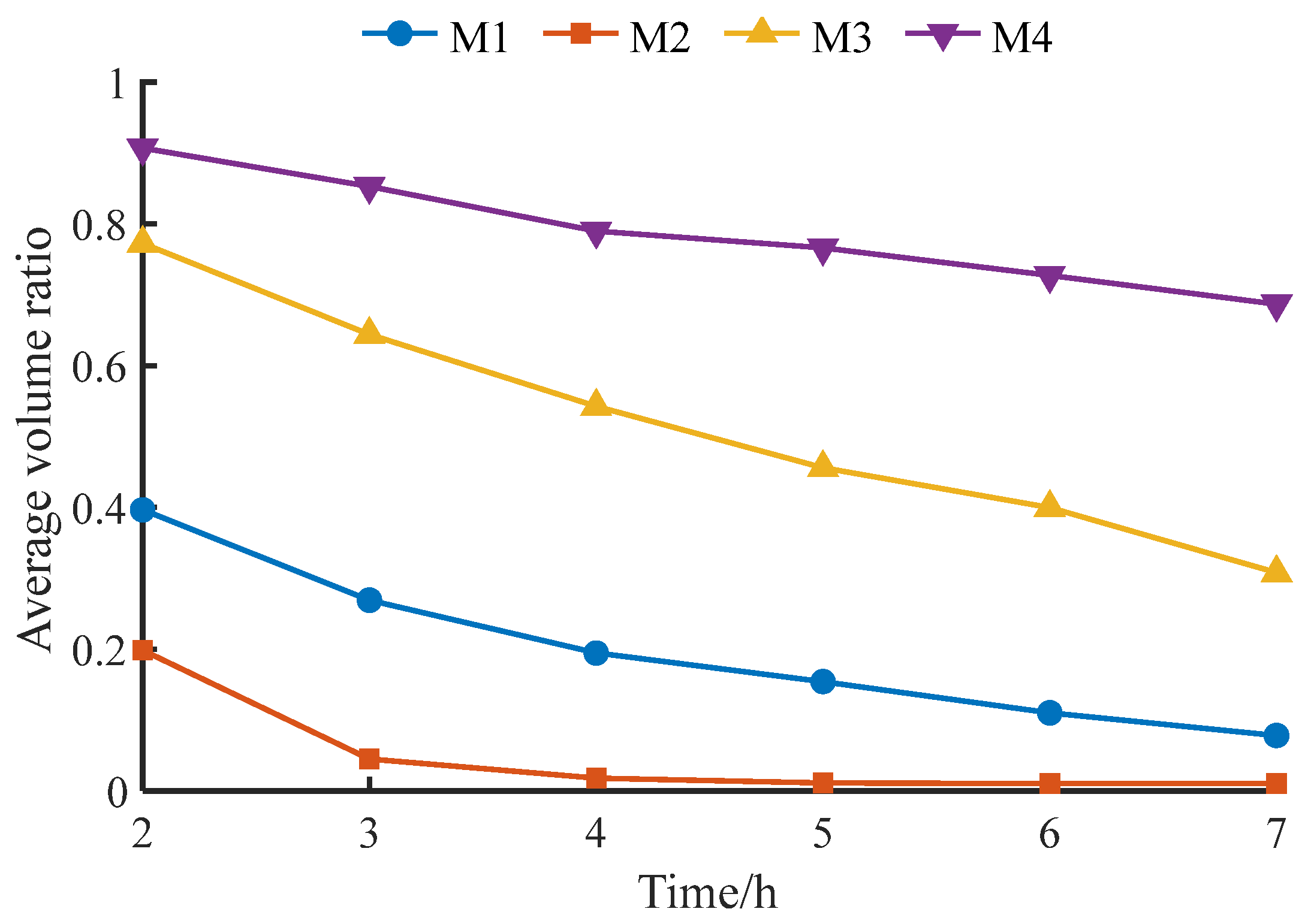
5.1. Comparative Analysis of Aggregation Methods

To verify the superiority of the zonotope inner approximation method adopted in this research in terms of the feasible region approximation accuracy, the following four feasible region approximation methods were compared:

M1: The virtual synchronous generator model approximation method proposed in [9].

M2: The virtual energy storage model approximation method proposed in [9].

M3: The basic isomorphic polyhedron approximation method proposed in [22].

M4: The improved zonotope approximation method adopted in this paper.

Considering the aggregation of 10 flexible resources under different time periods, the upper and lower power limits for each period are shown in Figure 3, and the regulation rates are listed in

Table 1. Regulation rates of 10 flexible resources.

Flexible Resource	Downward Regulation Rate/(kW/h)	Upward Regulation Rate/(kW/h)
1	3.5	3.5
2	4.8	4.8
3	5.4	5.4
4	5.0	5.0
5	4.0	4.0
6	6.6	6.6
7	5.2	5.2
8	5.1	5.1
9	5.4	5.4
10	5.2	5.2

. The energy constraints are omitted here, and it was assumed that the system frequency regulation capacity requirements were identical across all periods. The volume ratio between the exact feasible region and the approximated feasible region was calculated. The average volume ratio of all resources, denoted as $V^{\mathrm{AVE}}$, was used as the evaluation metric for the feasible region approximation accuracy. Its calculation method was as follows:

$$\begin{array}{c}{V}^{\mathrm{AVE}}={\displaystyle \frac{{\displaystyle \sum _{i=1}^n\frac{{\tilde{V}}_i}{V_i}}}{n}}\end{array}$$

(60)

where ${\tilde{V}}_i$ is the volume of the maximum inner approximated feasible region for resource $i$ and $V_i$ is the volume of the actual exact feasible region for resource $i$.

The average volume ratios of the four feasible region approximation methods under $T=2,3,\dots ,7$ were calculated, and the results are shown in Figure 4. To emphasize the differences in the approximation accuracy, the selected parameters featured large variations in the load power upper limits over time and significant differences in the regulation rates among the loads. Consequently, the feasible regions of different resources exhibited diverse shapes, and all four methods suffered from obvious feasible region losses. M1 and M2 modeled the approximated feasible regions as inscribed cubes and inscribed right pyramids, respectively, without considering the actual shapes of the feasible regions, resulting in substantial losses. The right pyramid in M2 deviated most from the actual feasible region, leading to the lowest approximation accuracy. M3 employed a basic isomorphic polyhedron that accounted for the actual shape of the exact feasible region, improving the approximation accuracy compared to M1 and M2. In contrast, the zonotope in M4 offered greater flexibility in translation and scaling, achieving the highest approximation accuracy. As the number of periods increased, the average volume ratios of all four methods decreased. This comparison demonstrated that the proposed method maintained a high approximation accuracy across different time periods. In addition, in the case of two time periods, the aggregation calculation time of M1–M4 was 3.99 s, 3.96 s, 3.97 s, and 4.00 s, respectively. It can be seen that the proposed method can significantly improve the approximation accuracy without increasing the calculation time.

5.2. Analysis of Day-Ahead Optimization Results

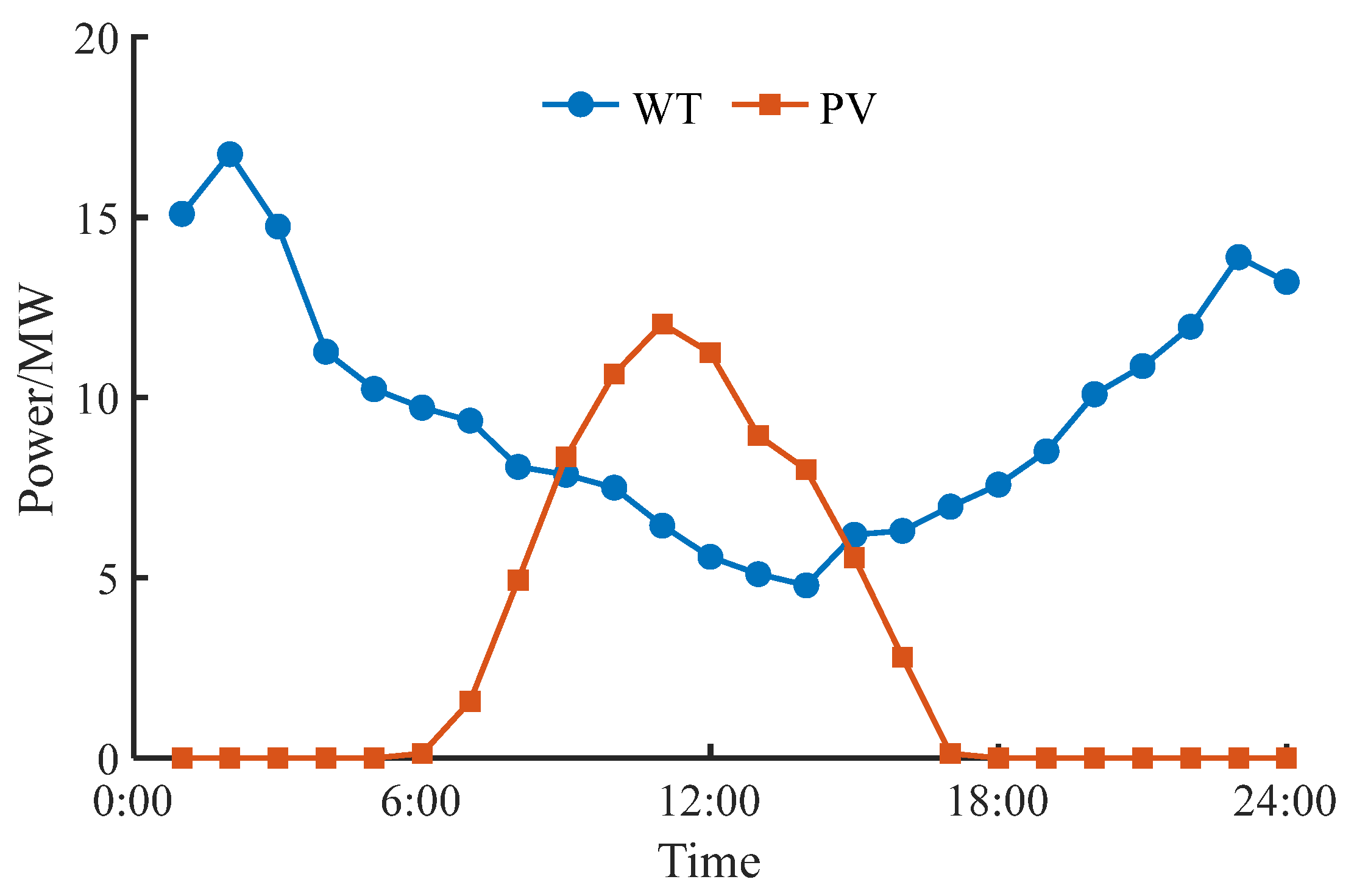
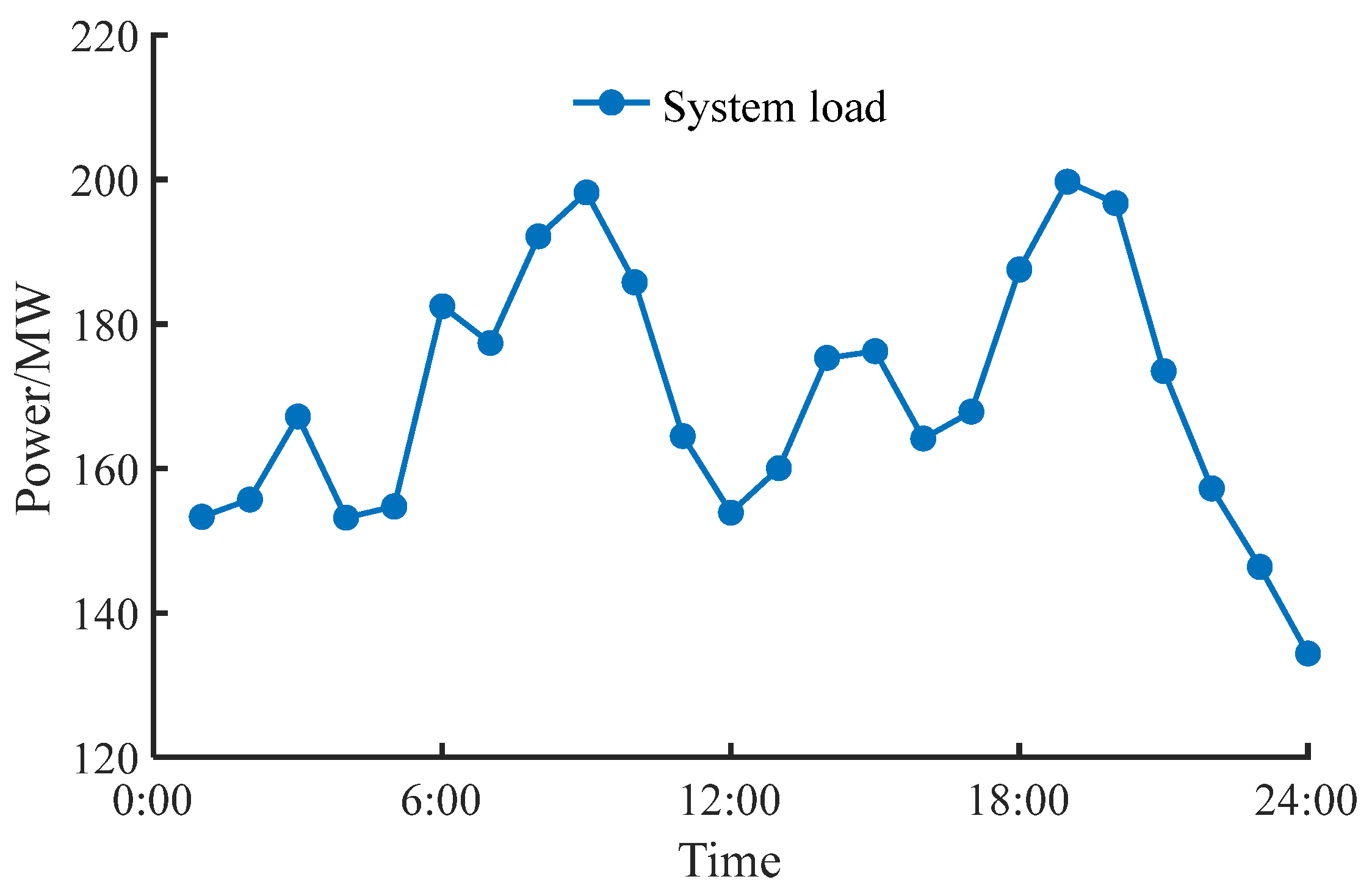
5.2.1. Case Data

The VPP considered in this paper was assumed to manage four clusters of flexible resources, including 500 electric vehicles, 500 thermostatically controlled loads, 500 industrial loads, and 1000 residential loads. The load parameters were referenced from [19]. The VPP participated in the electricity market and frequency regulation ancillary service market alongside five GSs. The day-ahead forecasted outputs of the WT and PV cells in the VPP are shown in Figure 5. The penalty prices for WT and PV curtailment were set to 0.5 CNY/kWh, and the compensation price for flexible resource dispatch was 0.45 CNY/kWh. The output limits of the GSs are listed in

Table 2. Upper and lower limits of output of GSs.

GS	Minimum Technical Output/MW	Maximum Technical Output/MW
G1	15	55
G2	20	75
G3	15	55
G4	10	35
G5	10	45

. The bidding information for the electricity market is provided in

Table 3. Bidding information of GSs in the electricity market.

GS	Capacity/MW			Price/(CNY/MWh)
	Segment 1	Segment 2	Segment 3	Segment 1	Segment 2	Segment 3
G1	20	15	15	370	455	548
G2	35	20	15	350	440	530
G3	25	10	15	361	464	559
G4	10	10	10	371	460	565
G5	20	10	10	360	445	540

using three-segment bids, and the bidding information for the frequency regulation market is listed in

Table 4. Bidding information of GSs in the frequency regulation market.

GS	Frequency Regulation Capacity		Frequency Regulation Mileage
	Capacity/MW	Price/(CNY/MWh)	Capacity/MW	Price/(CNY/MWh)
G1	4.5	190	45	19
G2	6.4	185	64	18.5
G3	4.5	200	45	20
G4	2.7	195	27	19.5
G5	3.6	180	36	18

. The VPP’s purchase/sale power upper limit was 15 MW, the electricity market bid upper limit was 1 CNY/kWh, the frequency regulation capacity bid upper limit was 0.35 CNY/kWh, the frequency regulation mileage bid upper limit was 0.035 CNY/kWh, and the minimum entry capacity for the frequency regulation market was 2 kW. The day-ahead forecasted system load curve is shown in Figure 6. The system frequency regulation capacity requirement was assumed to be 10% of the total system load, with a frequency regulation mileage-to-capacity ratio of 10.

The simulations were conducted on a Lenovo computer with a 1.80 GHz Intel (R) Core (TM) i7-8550U processor and 16 GB of RAM. The optimization problem was solved using the YALMIP 2023.06.22 toolbox in MATLAB R2023b, invoking the GUROBI 10.0.1 solver.

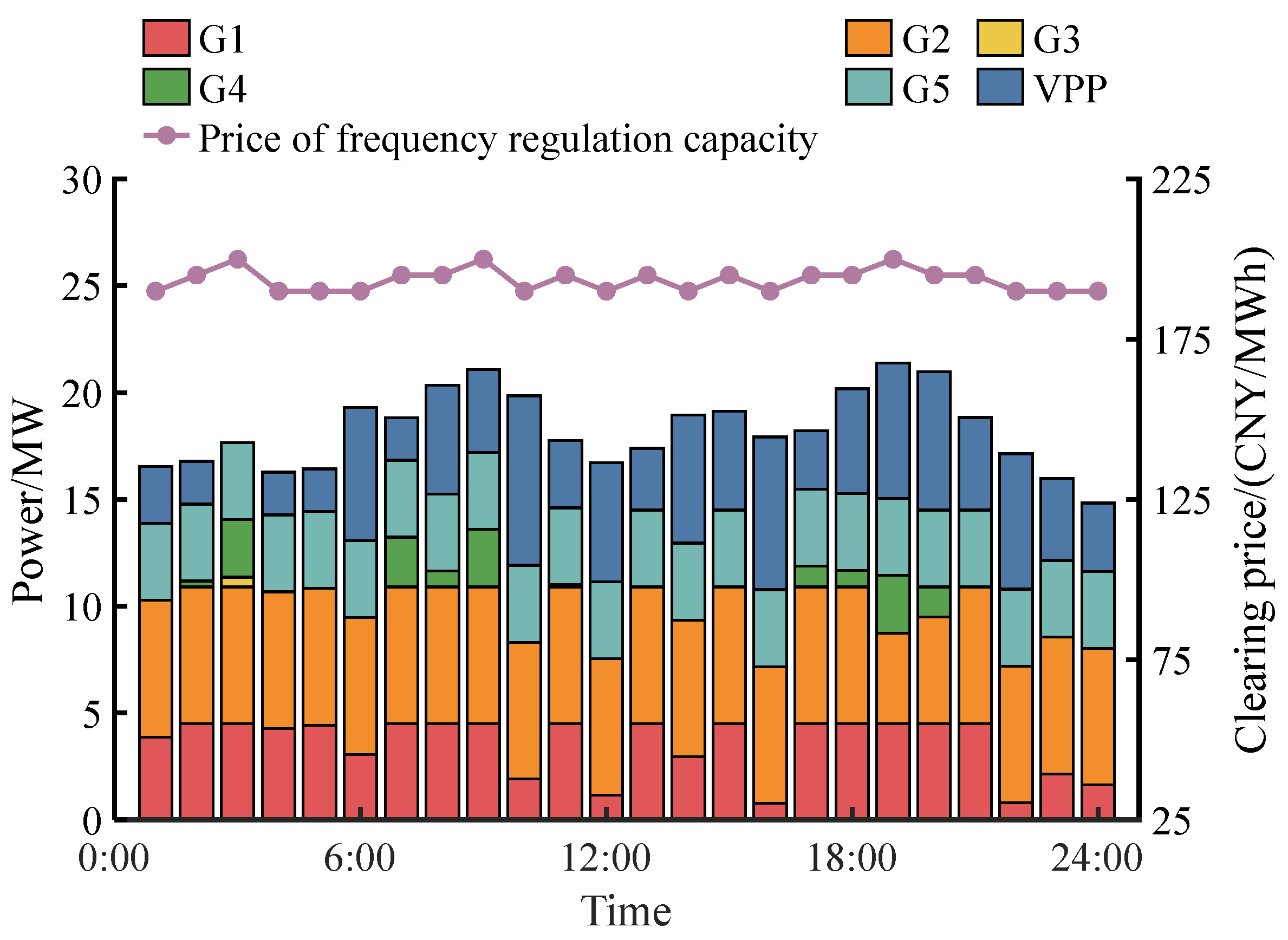
5.2.2. Analysis of Day-Ahead Market-Clearing Results

The electricity market-clearing results and the frequency regulation capacity/mileage clearing results are shown in Figure 7, Figure 8 and Figure 9. Figure 7 indicates that, in the electricity market, the grid’s overall load was substantial. Since the VPP’s internal load demand was primarily met by internal renewable energy, the VPP’s purchase/sale volumes had a minor impact on the overall clearing price. The system load demand was mainly satisfied by GSs. The system’s electricity clearing price aligned with the load variation trend, directly reflecting the market demand. Due to the three-segment bids from GSs in the electricity market, the clearing prices varied significantly across periods. During 6:00–11:00, 15:00–16:00, and 18:00–21:00, when the load demand was high, the third segment of the GSs’ bids was accepted, leading to notable price increases.

Figure 8 and Figure 9 show that the flexible resources in the VPP possessed significant regulation potential. The VPP can occupy a large share in the frequency regulation market as a frequency regulation resource. Its bidding strategies influenced the clearing prices in the frequency regulation market. By strategically adjusting the bid power and prices, the VPP can act as the marginal unit to maximize profits. During 2:00–4:00, 7:00–10:00, 11:00–12:00, and 17:00–21:00, when the system frequency regulation demand was high, G3 and G4 with higher bids were selected, and the VPP adopted the same bid price as the marginal unit.

The day-ahead dispatch results of the internal VPP resources are shown in Figure 10. During 1:00–4:00, the WT output was high, and during 8:00–15:00, the PV output was high. The VPP sold electricity to the grid to gain revenue while improving the renewable energy consumption rates. During 6:00–7:00 and 16:00–24:00, when the user demand was high, but the renewable energy output was low, the VPP purchased electricity from the grid to meet the load demand. By participating in both the electricity market and the frequency regulation ancillary service market, the VPP optimally scheduled internal demand-side flexible resources and renewable energy, balancing participation choices and participation levels across joint markets to maximize profits.

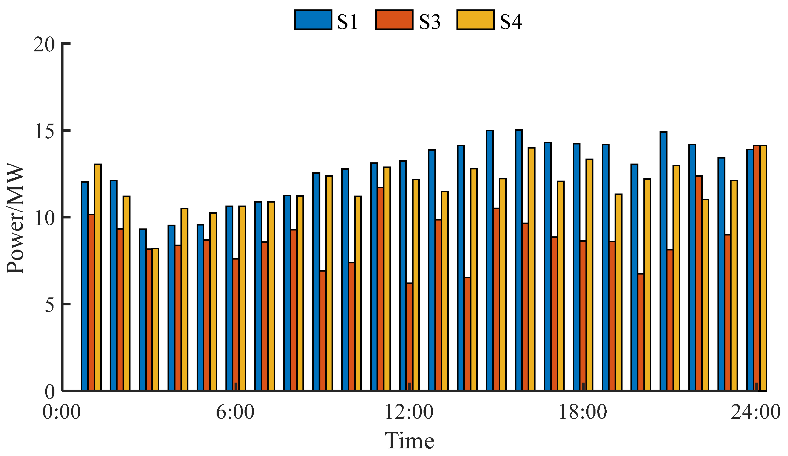
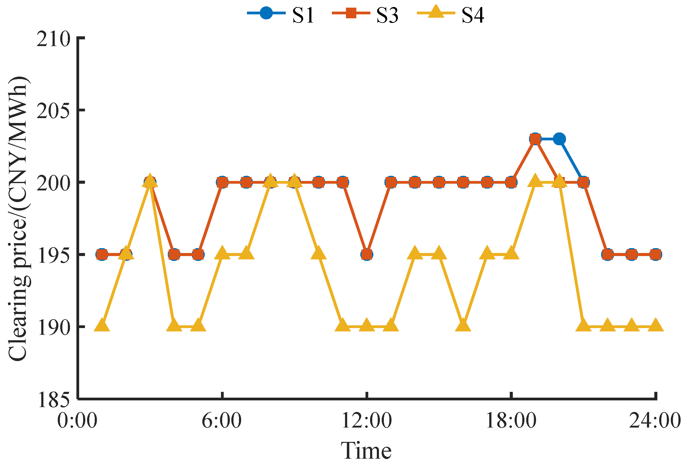
5.2.3. Comparative Analysis

To validate the effectiveness of the proposed improved zonotope approximation method and the day-ahead bidding model, the following five scenarios were compared:

S1: Flexible resources do not participate in regulation; the VPP participates in the electricity market.

S2: Flexible resources participate in regulation individually; the VPP participates in both the electricity and frequency regulation markets.

S3: Aggregated flexible resources participate in regulation; the VPP participates in the electricity market, with the feasible region approximation objective function ignoring grid regulation requirements.

S4: Aggregated flexible resources participate in regulation; the VPP participates in both markets, with the feasible region approximation objective function ignoring the grid regulation requirements.

S5: Aggregated flexible resources participate in regulation; the VPP participates in both markets, with the feasible region approximation objective function considering the grid regulation requirements.

The calculation results under different scenarios are compared in

Table 5. Comparison of calculation results of S1–S5.

Scenarios	VPP Revenues/CNY	Market Clearing Costs/CNY	Solution Time/s
S1	−3970.56	1,769,808	3.61
S2	31,645.02	1,770,069	1427.27
S3	−2054.60	1,770,364	3.95
S4	28,709.30	1,769,699	5.73
S5	31,006.84	1,769,732	5.63

.

The day-ahead dispatch results of the flexible resources, electricity market bidding results, and frequency regulation capacity clearing prices for S1, S3, and S4 are shown in Figure 11, Figure 12 and Figure 13.

When comparing S1 and S3 after aggregating flexible resources for regulation, the VPP reduced power purchases during periods with a low renewable energy output and increased power sales during periods with a high renewable energy output by implementing load curtailment across all periods, on the basis of meeting the power demand of flexible resources. This reduced the VPP’s operational cost from CNY 3970.56 to CNY 2054.60.

When comparing S1, S3, and S4, the VPP tended to utilize flexible resources for frequency regulation bids, since it gained higher revenues from participating in the frequency regulation market. Thus, the electricity bidding strategies in S1 and S4 were similar, but S4 achieved significantly higher revenue. As the VPP provided a large share of frequency regulation resources, its participation lowered the frequency regulation capacity clearing price, alleviating the grid frequency regulation demand pressure. Similar trends were observed for the frequency regulation mileage clearing prices.

The VPP’s frequency regulation capacity awards and system frequency regulation demand for S4 and S5 are shown in Figure 14. The total daily frequency regulation capacities for S4 and S5 were 91.05 MW and 101.41 MW, respectively. When comparing the revenues of S4 and S5, incorporating grid regulation requirements into the feasible region approximation objective function enhanced the frequency regulation capability of the flexible resources and increased the VPP revenue.

In S5, the calculation time of the feasible region aggregation of the four clusters was 481.74 s, 479.71 s, 455.68 s, and 957.96 s, respectively. Since the aggregation calculation of the four clusters can run separately and in advance, the total computation time of S5 was significantly less than that of S2. When comparing the computation times and revenues of the VPP for S2 and S5, S5 yielded a slightly lower revenue than S2, but significantly reduced the optimization time. Compared to individual participation, aggregated flexible resource regulation sacrificed a small amount of regulation capability and total revenue, but offered computational efficiency advantages by reducing the decision variables, making it suitable for large-scale aggregation. Considering both the economic performance and computational efficiency, the proposed method demonstrated rationality and effectiveness. Additionally, aggregated participation protects user load information privacy.

6. Conclusions

To maximize the regulation potential of flexible resources and achieve the efficient unified scheduling of flexible resource clusters in VPPs, this study proposed a VPP flexible resource aggregation method and a day-ahead bidding strategy for electricity and frequency regulation markets. This case study yielded the following conclusions:

• The improved zonotope-based feasible region approximation method enhanced the approximation accuracy, improved the frequency regulation capability of flexible resources, and increased the VPP revenue.
• The proposed day-ahead optimization model guided the VPP to participate in electricity and frequency regulation ancillary service markets, optimally scheduling internal flexible resources and renewable energy to maximize revenue.
• VPP participation in the frequency regulation market reduced the clearing prices and alleviated the frequency regulation resource demand pressure.

Coordinated optimization and bidding strategies for VPP participation in multiple ancillary services, bidding strategies considering uncertainty and resilience, and feasible region aggregation methods suitable for asymmetric regulation scenarios are directions for future research.

References

1. Liu, Z.; Guo, G.; Gong, D.; Xuan, L.; He, F.; Wan, X.; Zhou, D. Bi-Level Game Strategy for Virtual Power Plants Based on an Improved Reinforcement Learning Algorithm. Energies 2025, 18, 374. [Google Scholar] [CrossRef]
2. Wang, K.; Xue, Y.; Shahidehpour, M.; Chang, X.; Li, Z.; Zhou, Y.; Sun, H. Resilience-Oriented Two-Stage Restoration Considering Coordinated Maintenance and Reconfiguration in Integrated Power Distribution and Heating Systems. IEEE Trans. Sustain. Energy 2025, 16, 124–137. [Google Scholar] [CrossRef]
3. Yang, N.; Zhu, L.; Wang, B.; Fu, R.; Qi, L.; Jiang, X.; Sun, C. A Master–Slave Game-Based Strategy for Trading and Allocation of Virtual Power Plants in the Electricity Spot Market. Energies 2025, 18, 442. [Google Scholar] [CrossRef]
4. Qi, J.; Ying, A.; Zhang, B.; Zhou, D.; Weng, G. Distributed Frequency Regulation Method for Power Grids Considering the Delayed Response of Virtual Power Plants. Energies 2025, 18, 1361. [Google Scholar] [CrossRef]
5. Gao, Y.; Ai, Q. Novel Optimal Dispatch Method for Multiple Energy Sources in Regional Integrated Energy Systems Considering Wind Curtailment. CSEE J. Power Energy Syst. 2024, 10, 2166–2173. [Google Scholar] [CrossRef]
6. Barot, S.; Taylor, J.A. A Concise, Approximate Representation of a Collection of Loads Described by Polytopes. Int. J. Electr. Power Energy Syst. 2017, 84, 55–63. [Google Scholar] [CrossRef]
7. Tong, Y.; Hu, J.; Du, H.; Chen, C.; Zeng, W. Feasible Region Aggregation Method for Load Regulation of Minkowski Heat Pump Based on External Approximation of VB Model. Dianwang Jishu/Power Syst. Technol. 2024, 48, 3340–3349. [Google Scholar] [CrossRef]
8. Wen, Y.; Hu, Z.; You, S.; Duan, X. Aggregate Feasible Region of DERs: Exact Formulation and Approximate Models. IEEE Trans. Smart Grid 2022, 13, 4405–4423. [Google Scholar] [CrossRef]
9. Li, Z.; Li, T.; Wu, W.; Zhang, B.; Jiang, F.; Cui, D. Minkowski Sum Based Flexibility Aggregating Method of Load Dispatching for Heat Pumps. Dianli Xitong Zidonghua/Autom. Electr. Power Syst. 2019, 43, 14–21. [Google Scholar] [CrossRef]
10. Chen, X.; Dall’Anese, E.; Zhao, C.; Li, N. Aggregate Power Flexibility in Unbalanced Distribution Systems. IEEE Trans. Smart Grid 2020, 11, 258–269. [Google Scholar] [CrossRef]
11. Wang, S.; Wu, W. Aggregation Reference Model and Quantitative Metric System of Flexible Energy Resources. Dianli Xitong Zidonghua/Autom. Electr. Power Syst. 2024, 48, 1–9. [Google Scholar] [CrossRef]
12. Müller, F.L.; Szabó, J.; Sundström, O.; Lygeros, J. Aggregation and Disaggregation of Energetic Flexibility from Distributed Energy Resources. IEEE Trans. Smart Grid 2019, 10, 1205–1214. [Google Scholar] [CrossRef]
13. Hreinsson, K.; Scaglione, A.; Alizadeh, M.; Chen, Y. New Insights from the Shapley-Folkman Lemma on Dispatchable Demand in Energy Markets. IEEE Trans. Power Syst. 2021, 36, 4028–4041. [Google Scholar] [CrossRef]
14. Chen, X.; Li, N. Leveraging Two-Stage Adaptive Robust Optimization for Power Flexibility Aggregation. IEEE Trans. Smart Grid 2021, 12, 3954–3965. [Google Scholar] [CrossRef]
15. Li, J.; Ai, Q. Operation Mode of Virtual Power Plant Considering Peak Regulation Auxiliary Service. Dianli Zidonghua Shebei/Electr. Power Autom. Equip. 2021, 41, 1–7. [Google Scholar] [CrossRef]
16. Qing, Z.; An, R.; Gao, H.; Gao, Y.; Wang, C.; Yang, J.; Liu, J. Intelligent Peak Regulation Pricing for Virtual Power Plant Considering Interactive Response of Distributed Resources. Dianli Zidonghua Shebei/Electr. Power Autom. Equip. 2023, 43, 96–103. [Google Scholar] [CrossRef]
17. Lee, J.; Won, D. Optimal Operation Strategy of Virtual Power Plant Considering Real-Time Dispatch Uncertainty of Distributed Energy Resource Aggregation. IEEE Access 2021, 9, 56965–56983. [Google Scholar] [CrossRef]
18. Li, X.; Zhan, Z.; Li, F.; Zhang, L. Bidding Strategy for Battery Swapping Station Participating in Electricity Energy and Frequency Regulation Market Considering Demand Response of Battery Swapping. Dianli Xitong Zidonghua/Autom. Electr. Power Syst. 2024, 48, 207–215. [Google Scholar] [CrossRef]
19. Xiao, F.; Cui, Y.; Zhu, J.; Qiao, Y.; Li, Z.; Ai, Q. A Load-Side Resource Aggregation Method Based on Minkowski Sum. J. Phys. Conf. Ser. 2024, 2728, 012073. [Google Scholar] [CrossRef]
20. Tiwary, H.R. On the Hardness of Computing Intersection, Union and Minkowski Sum of Polytopes. Discret. Comput. Geom. 2008, 40, 469–479. [Google Scholar] [CrossRef]
21. Zhou, H.; Liu, Y.; Chen, Y.; Wang, Z.; Qu, S.; He, K. Demand Side Feasible Region Aggregation Considering Flexibility Revenue. Electr. Power 2022, 55, 56–63. [Google Scholar]
22. Yi, Z.; Xu, Y.; Gu, W.; Yang, L.; Sun, H. Aggregate Operation Model for Numerous Small-Capacity Distributed Energy Resources Considering Uncertainty. IEEE Trans. Smart Grid 2021, 12, 4208–4224. [Google Scholar] [CrossRef]
Figure 1. Flow chart of research methodology.
Energies 18 02458 g001
Figure 2. Schematic diagram of similarity.
Energies 18 02458 g002
Figure 3. Upper and lower limits of power of 10 flexible resources in each period.
Energies 18 02458 g003
Figure 4. Comparison of approximation accuracy of four feasible region approximation methods in different time periods.
Energies 18 02458 g004
Figure 5. Day-ahead predicted output of WT and PV cells.
Energies 18 02458 g005
Figure 6. Day-ahead predicted curve of system load.
Energies 18 02458 g006
Figure 7. Day-ahead clearing results of electricity market.
Energies 18 02458 g007
Figure 8. Day-ahead clearing results of frequency regulation capacity.
Energies 18 02458 g008
Figure 9. Day-ahead clearing results of frequency regulation mileage.
Energies 18 02458 g009
Figure 10. Day-ahead scheduling results of flexible resources in VPPs.
Energies 18 02458 g010
Figure 11. Day-ahead scheduling results for flexible resources of S1, S3, and S4.
Energies 18 02458 g011
Figure 12. Day-ahead bidding results for electricity market of S1, S3, and S4.
Energies 18 02458 g012
Figure 13. Day-ahead clearing price for frequency regulation capacity of S1, S3, and S4.
Energies 18 02458 g013
Figure 14. Frequency regulation demand and frequency regulation capacity of the VPP in S4 and S5.
Energies 18 02458 g014