1. Introduction
Quantum computing represents a paradigm shift in computational capabilities, leveraging principles of quantum mechanics to process information in fundamentally different ways from classical computing. Traditional computers use binary bits as the basic unit of data, which can either be a zero or a one. In contrast, quantum computers use quantum bits, or qubits, which can exist in multiple states simultaneously, thanks to the phenomena of superposition and entanglement [
1]. This allows quantum computers to process a vast number of possibilities concurrently, offering potential exponential speed-ups for certain computational tasks, for example, in factoring large integer numbers [
2] or in searching unstructured database [
3,
4].
Recent advancements in quantum hardware [
5,
6,
7] and the development of sophisticated algorithms [
8,
9,
10,
11] have made quantum computing a highly promising area of research. These advancements make quantum computing a promising field for a variety of applications, particularly in areas that require handling complex, high-dimensional datasets or simulations where classical computers struggle.
One of the pivotal developments in this field is the Quantum Neural Network (QNN) [
12,
13]. QNNs integrate the principles of quantum computing with the architectural concepts of classical neural networks. This hybrid approach has been explored for various applications, including drug discovery, financial modeling, and, notably, complex system simulations such as those needed in power systems.
Quantum computing has been explored for various power system applications, including power flow analysis [
14], unit commitment [
15], system reliability [
16], and stability assessment [
17]. There is a burgeoning body of literature, as indicated by several review papers [
18,
19,
20], that discusses the integration of quantum computing into power system operations, underscoring the participation of entities such as the Department of Energy (DOE) and various utility companies in these research efforts.
Simulation of power systems is of paramount importance for ensuring their stability, efficiency, and reliability [
21,
22,
23,
24], particularly as the integration of renewable energy sources like wind and solar continues to expand. These renewables are incorporated into power systems through power electronic devices, such as inverters, which necessitate the simultaneous handling of both small and large time steps in simulations. This is due to the rapid responses of the power electronic devices contrasted with the slower-moving dynamics of synchronous generators. Accurate modeling of these diverse dynamics is essential for effective grid management and planning, highlighting the critical need for robust simulation tools capable of managing complex interactions across varying time scales.
The simulation of power systems typically involves solving differential-algebraic equations (DAEs), which describe both the dynamic behavior and the algebraic constraints within the electrical network. Traditional approaches for these simulations include numerical methods such as Euler’s and Runge–Kutta methods [
25], which discretize the equations to approximate solutions, and semi-analytical methods [
23,
26], which combine analytical and numerical techniques for improved accuracy. More recently, Physics-Informed Neural Networks (PINNs) [
27] have been applied to solve differential equations (DEs) by training neural networks to adhere to the underlying physics of the systems, thus providing a data-driven approach to simulation.
However, each of these methods has its limitations. Numerical and semi-analytical methods can become computationally intensive and may not scale efficiently with the increasing complexity of modern power systems. PINNs, while innovative, often require extensive data and computational resources, as they rely on classical neural networks that utilize a large number of parameters to capture complex functions.
In this context, QNNs present a promising alternative. QNNs leverage the principles of quantum mechanics to perform computations, utilizing a smaller number of parameters than classical neural networks to represent nonlinear functions [
12]. This reduction in parameters can potentially lead to more efficient simulations, as QNNs could process complex computations faster and with higher precision due to quantum superposition and entanglement.
Beyond the reduced parameterization and expressive power of QNNs, an emerging body of research suggests that QNNs possess strong generalization abilities and resilience against overfitting–especially in nonlinear settings [
28]. This is highly relevant in power system simulations, where dynamic behaviors vary across operating scenarios and overfitting to specific conditions can lead to unreliable models. These properties, combined with the potential for quantum-enhanced speedups, make QNNs a promising alternative to conventional solvers for DAEs in power systems.
Quantum computing has been applied to solve DEs and Partial Differential Equations (PDEs) [
29]. However, its potential to solve DAEs remains largely unexplored. Therefore, this paper takes a pioneering step by investigating the use of QNNs to address the challenges in power system simulation. This exploration is the first of its kind and aims to demonstrate how quantum-enhanced computational models can solve the simulation of complex power systems.
The rest of the paper is organized as follows.
Section 2 provides a description of the DAEs for the two small power systems simulated.
Section 3 offers a general overview of the QNN.
Section 4 details the two types of QNNs used to solve the power system simulation problems.
Section 5 presents the simulation results. Finally, conclusions are given in
Section 6.
2. Problem Description: DAE
DAEs are integral to modeling dynamic systems where constraints intertwine the derivatives of some variables with the algebraic relationships among others. DAEs are prevalent across a diverse array of fields, including electrical circuit design, mechanical system simulation, chemical process modeling, and economic dynamics. This wide applicability underlines the importance of understanding their structure, challenges, and solution methods.
DAEs are characterized by their differentiation index, a critical measure that indicates the complexity of numerical solutions. The differentiation index describes the number of times an equation must be differentiated to convert it into an ordinary differential equation (ODE), affecting the choice of numerical methods for solving the DAE. Common forms of DAEs include semi-explicit, where some equations involve derivatives explicitly, and fully implicit, where derivatives may not be explicitly present.
Boundary and initial conditions play pivotal roles in solving DAEs, providing the necessary constraints to ensure unique and stable solutions. Proper formulation of these conditions is crucial, as inconsistent or inadequate initial conditions can lead to non-converging solutions.
Here, we provide a generalized expression of DAEs.
We define the set
as follows:
where
t represents the independent variable, typically time.
denotes the ith dependent variable as a function of t.
represent the first, second, and up to the th order derivatives of , where is the highest order of derivative for the ith variable.
Subsequently, the DAE system can be succinctly expressed as:
where
symbolizes the functions delineating the interrelations within the DAE system. Each corresponds to the jth equation in the system.
denotes the number of equations in the DAE system, indicating the size of the system.
Boundary conditions are essential for constraining the solution space of DAE systems. They are articulated as a series of equations that the solution must satisfy at predetermined points within the domain, not limited to its boundaries. Formally, these conditions are given by:
where
denotes the kth boundary condition function, which applies to the system state at a critical point within the domain.
represents the total number of boundary conditions enforced on the system.
3. A Unified Quantum Neural Network Framework for DAEs
In solving DAEs, our approach employs QNNs, aiming to approximate the solutions
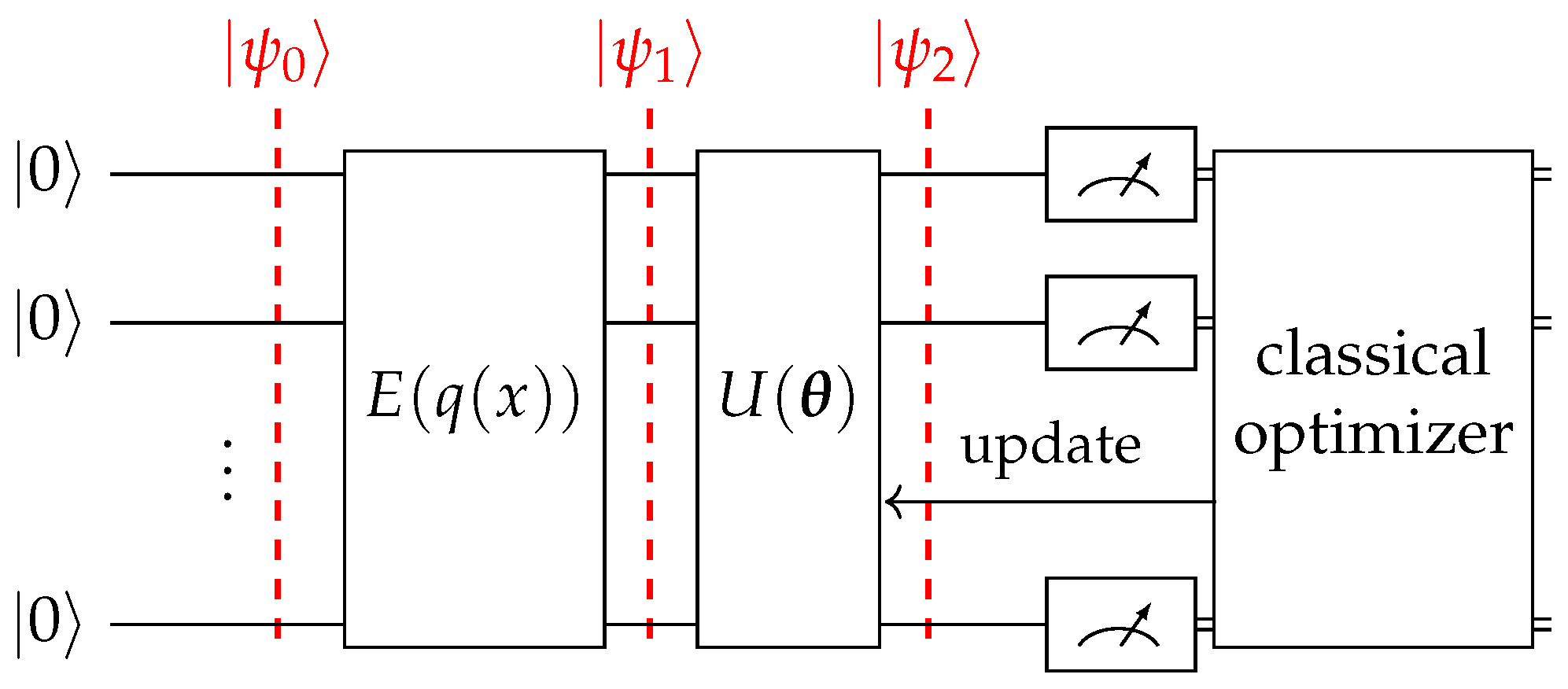
. These QNNs encompass several components: data encoding, a parameterized ansatz, measurement, and a classical optimizer. Each of these components are elaborated on in later sections of this paper. The methodology primarily involves iteratively updating the circuit parameters. This process is continued until the error in the computed solution, based on the circuit’s output, is reduced to a satisfactory level within the context of the DAE equations. An in-depth illustration of the QNN’s architecture, particularly its iterative parameter update mechanism, is presented in
Figure 1.
From a high-level perspective, this approach comprises two distinct segments: the quantum segment and the classical segment.
3.1. Quantum Segment
To initiate the process, we start with a quantum state represented as:
where
n is the number of qubits in the circuit. We then embed our classical input
x into the circuit through a quantum operator
, as expressed in Equation (
4).
The encoding function
serves as a preprocessing step for the classical input before it is embedded into the quantum circuit. Next, a parametric multi-layer quantum ansatz operator
is applied to make the circuit trainable.
The
is a matrix of parameters and can be written as
where
represents the parameter in the
qubit and in the
layer.
3.2. Classical Segment
The solution
is considered a function of the expectation value of an observable
from the final state of the circuit (
). Mathematically, this is given by:
where
g represents the post-measurement function applied to
M, approximating the value of the function. Subsequently, the quantum models are trained by updating and optimizing the parameter
with a classical optimizer guided by a loss function. This loss function comprises two parts, providing a measure of the solution’s accuracy.
The first part assesses the discrepancy between the estimated and true boundary values. This is quantified using (
9), where
denotes the total boundary points.
Here,
is derived from the boundary conditions specified by problem (
1), while
is obtained from the quantum circuit, as described in (
8).
The second part assesses the degree to which the approximated solutions satisfy the system of DAEs (
1) for
training points. It is expressed as:
Here,
denotes the number of DAEs in the system.
Finally, the total loss is computed as a weighted sum of the two components, reflecting the relative importance of boundary accuracy and training point adherence. This is expressed as:
In this equation, and are tuning coefficients. These coefficients are adjustable parameters that allow for the fine-tuning of the model, enabling the prioritization of either boundary accuracy () or adherence at the training points (). The choice of these coefficients depends on the specific requirements and goals of the model, as well as the characteristics of the problem being addressed.
3.3. Classical Optimizer
We explored several classical optimizers, including Stochastic Gradient Descent (SGD), Adam optimizer, Broyden–Fletcher–Goldfarb–Shanno (BFGS), Limited-Memory BFGS (L-BFGS), and Simultaneous Perturbation Stochastic Approximation (SPSA).
Among these optimizers, BFGS stands out for its fast convergence and robustness in handling non-convex landscapes, making it advantageous in scenarios with saddle points and flat regions [
30]. SGD is computationally efficient but may converge slowly [
31]. The Adam optimizer offers adaptive learning rates but can exhibit erratic behavior in high-dimensional landscapes [
32]. SPSA, on the other hand, is a gradient-free optimizer suitable for optimizing circuits subject to noise [
33].
Given the nature of our problem, we opted for the BFGS optimizer to enhance the performance of our QNN circuit. Its capability to navigate non-convex landscapes aligns seamlessly with the intricacies and challenges inherent in our problem domain. Nevertheless, it is imperative to underscore that the choice of an optimizer should be contingent upon the specific demands and constraints of the given problem.
For instance, if the hardware introduces noise, the SPSA optimizer might prove more effective. It is crucial to evaluate the unique attributes of the problem and select an optimizer accordingly to ensure optimal performance. In this study, we utilized ideal simulators devoid of noise, and we opted for BFGS based on the elucidated reasons.
4. QNN Architectures for Power System Simulation
The implementation of the proposed approach necessitated a pivotal consideration: the selection of a quantum model. This model should not only exhibit expressive capabilities but also closely align with the function it is intended to approximate. In the realm of quantum computing, certain global approximator models, such as Haar Unitary, have been proposed. However, their extensive complexity and the vast parameter space required for training them make them less effective. These models often exhibit weak performance, are highly susceptible to encountering saddle-point issues, and may become trapped in local minima during the optimization and training process [
34,
35].
In this paper, we leveraged the physics information inherent in power system equations to design quantum models. These models feature generative functions that closely mimic the shapes of power system simulation functions. Consequently, the optimization process becomes significantly more efficient. Power systems involve two distinct types of functions: those characterized by fluctuations and sinusoidal patterns, requiring a model adapted to these features, and those amenable to polynomial fitting, such as power-series and Chebyshev functions.
For sinusoidal-friendly models, we employed our previously proposed Sinusoidal-Friendly QNN (SFQ). Additionally, for polynomial-friendly functions, we introduced a novel and promising quantum model named Polynomial-Friendly QNN (PFQ). PFQ harnesses the power of quantum superposition, offering the potential for quantum advantage.
To clearly link the proposed QNNs with the power system transient simulation problem, we emphasize how each QNN approximates solutions to specific DAE components. The DAEs governing power systems, as shown in Equations (
A1) to (
A3) for the SMIB system and Equations (
A4) to (
A9) for the 3-machine system, model the time evolution of rotor angle
and speed deviation
.
The QNNs were trained to learn these time-dependent state variables by approximating the functions
and
using quantum circuits that minimized DAE residuals and boundary mismatches, as defined in Equations (
9)–(
11). The Sinusoidal-Friendly QNN (SFQ) was particularly suited to learn the sinusoidal behaviors, which reflect oscillatory generator dynamics. In contrast, the Polynomial-Friendly QNN (PFQ) better matched the slowly varying or polynomial-like behaviors.
Thus, each QNN architecture was designed with physical interpretability in mind, aligning its structure with the mathematical form of power-system DAEs, ensuring the learned quantum model respected the physics of the underlying system.
In the upcoming section, we delve into the properties of quantum segments for these specific QNNs utilized in our study.
4.1. Structure 1—Sinusoidal Friendly QNN (SFQ)
The first QNN we utilized was the one we previously explored in [
12] for sinusoidal-friendly functions. We proved that this QNN could efficiently approximate sinusoidal and fluctuating functions. Here, we explain the structure of the circuit we used and leave the details of the expressivity of the model to the paper we mentioned [
12].
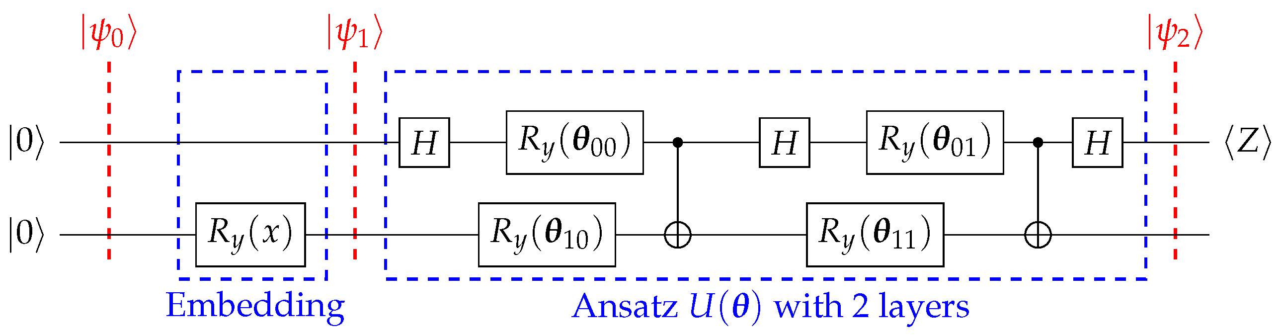
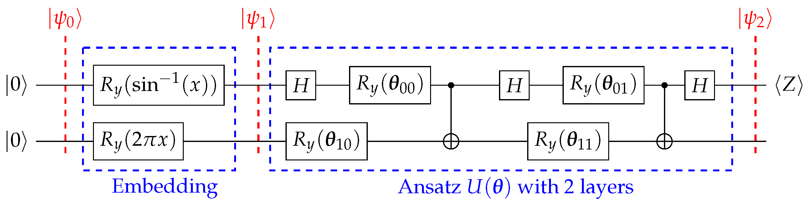
For SFQ, we employed two different kinds of embedding:
embedding (
Figure 2), and
embedding (
Figure 3).
4.1.1. Embedding
For this type of embedding, we considered two qubits with
and
4.1.2. Embedding
For the
embedding in the SFQ structure, we also considered two qubits, but this time
and,
To implement the quantum ansatz
, we used a series of layers to train the circuit, fitting it to approximate the solution of our DAE. The ansatz consisted of
L layers, and the flexibility and variance of our circuit depended on
L [
12]. The more layers, the more time and data points we needed to train it, so the demand on the number of layers depended on the complexity of our function to approximate [
12].
The observable
for this structure is
, where
H is a Hadamard gate,
Z is the Pauli-Z matrix, and
I is the identity matrix. The post-processing function
g in this structure is [
12]:
Assuming that the expectation value of our observable is
, then we have
4.2. Structure 2—Polynomial Friendly QNN (PFQ)
We propose an innovative model harnessing quantum principles in QNNs, which exhibit exceptional suitability for approximating functions represented by power series and polynomials. Assume the ultimate solution of a DAE is expressed as:
Subsequently, we define
as
where
n is the number of qubits. Afterward, we define the quantum embedding operator
as:
where
.
The construction of the operator
is described in [
36], where researchers developed an effective method for quantum state preparation using measurement-induced steering, enabling the initialization of qubits in arbitrary states on quantum computers. Ultimately, a quantum ansatz operator
is utilized to produce a subset of the power series, as expressed in Equation (
20).
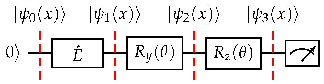
4.3. Simplified PFQ Form with
To illustrate this process for a single qubit, let us consider an
gate as in Equation (
21).
The corresponding quantum circuit with one rotation gate is depicted in
Figure 4.
Assuming we set
m to 1 in Equation (
19), we obtain:
The
is defined as:
By substituting Equations (
22) and (
23) into Equation (
21), we obtain:
Now, let us calculate the probability
:
After some trigonometric simplifications on
, we obtain:
Multiplying
by
yields:
Equation (
26) can be abstracted as:
where
This expression can be viewed as a segment of a quadratic power series. However, it encounters some limitations, which we address subsequently.
4.4. Enhanced PFQ Version with
Initially, the limitation of a simple PFQ concerns the restricted range of , specifically, . Secondly, the range of is also constrained within .
To mitigate these constraints, we propose the incorporation of two classical adjustable parameters, enhancing the adaptability of the approximating function. Consequently, we define the output as:
Here, stands as a classical trainable parameter, whereas may either be a physics-informed constant, tailored to the problem’s boundary conditions, or a trainable parameter. In cases where the boundary conditions are undefined, opting for a trainable is advisable.
With these adjustments, we obtain:
and
As a result, the range of extends to the entire set of real numbers , and falls within the interval .
The third limitation is that the range of
is limited,
. With the solution of the second limitation, we mitigate the problem of not having negative coefficients for
since we have added
, which can create a negative coefficient for
. However, we still need to improve it and make it more expressive to have both negative and positive coefficients for
. To do this, we can add some rotation gates to add the degree of freedom for the coefficients. As an example, consider we add an
gate after the
gate, as shown in
Figure 5. Then, we have:
By substituting
from Equation (
24) to (
28), we obtain:
Consequently, substituting
from Equation (
30) into (
31) and multiplying both sides by
yield:
which shows that we have
and
in
. This implies that when calculating the probability of 1, terms like
can appear, resulting in both negative and positive coefficients of
.
For simplicity, we assumed the same
for both
and
. However, it is also possible to consider different
values (e.g., see
Figure 6) to enhance the model’s trainability. Additionally, the introduction of more gates generates additional terms, enabling the model to express a broader range of power series with the same degree.
To evaluate the function to be approximated through this method, we use the same approach as in Equation (
8), where
O is the expectation value of
Z for the first qubit. The expectation value can be calculated as follows:
Here, we have both
and
, incorporating different coefficients for power series of degree 2.
4.5. Scalability and Advantage of PFQ
PFQ’s scalability is facilitated by increasing the number of qubits, as outlined in Equation (
19). Specifically, augmenting the qubit count,
n, exponentially increases the polynomial’s degree,
m, where
. Furthermore, the introduction of entanglement between qubits, alongside additional rotation gates, enhances the degree of freedom for the coefficients of the generated independent terms in our polynomials. In fact, this approach enables the model to effectively tackle more complex systems by employing extra qubits, thereby extending the degrees of the power series.
Another critical aspect to note is that the output from our PFQ circuit undergoes post-processing, expressed as
where
and
are classical parameters, and
represents quantum parameters, with
denoting the expectation value of the observable
Z for the first qubit. Consequently, the algorithm involves two classical parameters and a flexible number of quantum parameters, enhancing its quantum scalability.
In real-world power systems, DAEs frequently involve strong nonlinearities (e.g., trigonometric relationships in rotor dynamics) and discontinuities (e.g., abrupt changes during faults or switching events). Our proposed QNN-based framework addresses these challenges through two mechanisms:
Nonlinearity adaptability: Both the SFQ and PFQ architectures are designed to approximate nonlinear behaviors. SFQ targets sinusoidal oscillations, while PFQ, with its polynomial basis, captures smooth nonlinear trends. The quantum encoding and trainable parameterized circuits enable the representation of complex function spaces with fewer parameters than classical NNs, enhancing approximation in nonlinear regions.
Discontinuity management via domain decomposition: For discontinuous phenomena (e.g., faults), we divide the simulation into sequential time segments—pre-fault, fault-on, and post-fault—with QNNs trained independently in each. This approach allows the model to reset its approximation locally, mitigating the impact of discontinuities.
Importantly, recent work (e.g., [
28]) has shown that QNNs exhibit strong generalization ability and robustness to overfitting, enabling them to maintain performance across training and testing phases even in complex nonlinear settings.
5. Results
This section presents the results of using various QNNs to solve DAEs. The QNNs were implemented on Pennylane [
37,
38] on the NCSA Delta high-performance computer (HPC). The BFGS optimizer was employed to optimize the parameters in the QNNs. Our simulations primarily addressed DAEs in power systems, focusing on one-machine and three-machine test systems. The details of their respective DAEs are given in
Appendix A and
Appendix B. In this study, no additional control mechanisms (e.g., excitation systems or PSS) were included. This design choice allowed us to focus on the fundamental response of the power system models and the QNNs’ capacity to approximate their dynamics. Results detail the performance of different QNN structures with different embedding methods (
Section 5.1), the setting of time interval and the number of training points (
Section 5.2 and
Section 5.3), and the solution of the entire period of the DAE (
Section 5.4).
5.1. QNN Structure and Embedding
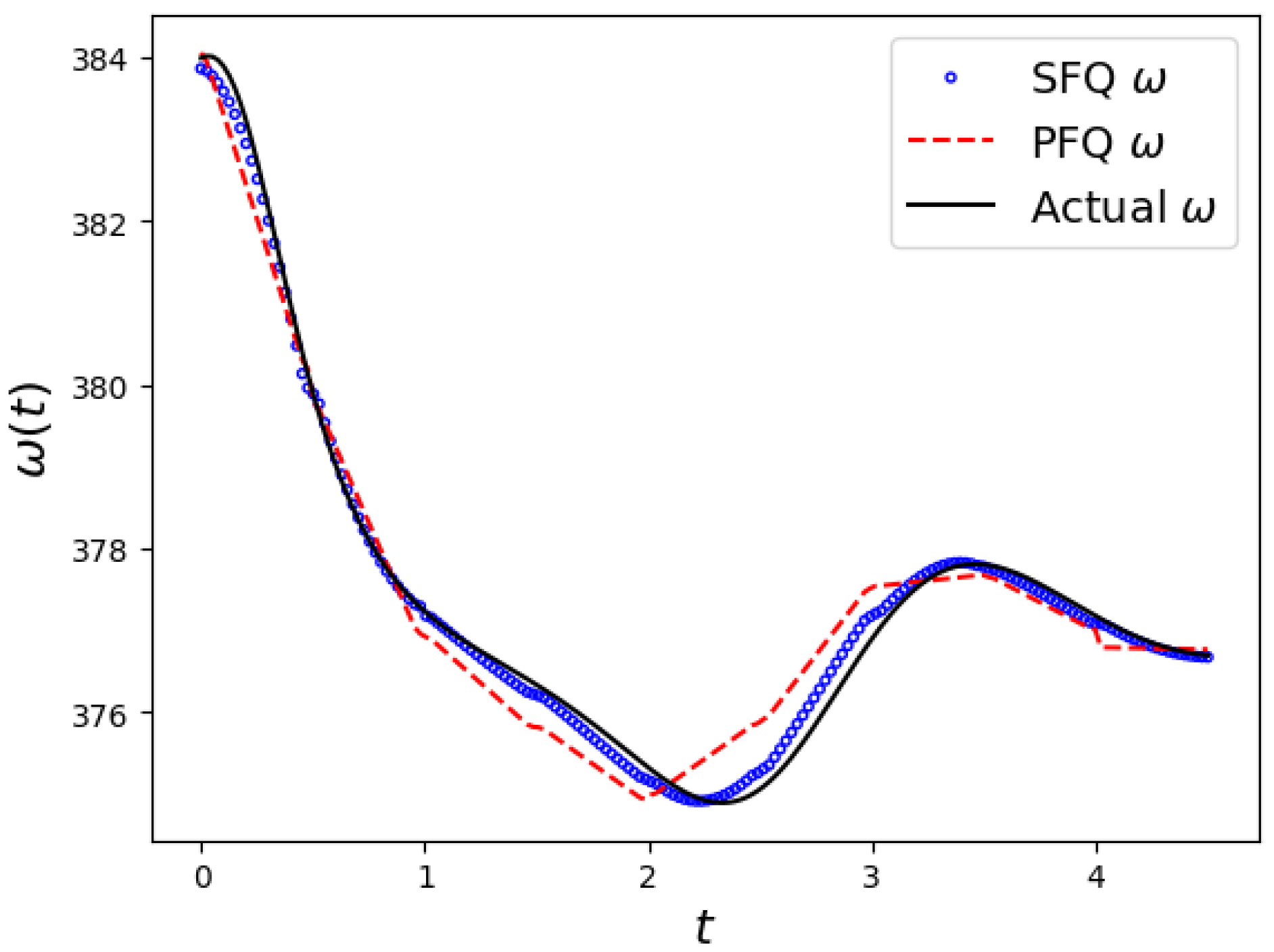
To analyze the efficacy of various QNN architectures, we initially focused on a single-machine DE over a 0.5-second interval (the setting of the time interval is discussed in the next subsection), utilizing 20 training points. The experimental conditions were kept constant, varying only in the QNN structure applied. As depicted in
Figure 7, the SFQ structure excelled in capturing the sinusoidal behavior inherent in the one-machine solution, achieving notably lower error compared to the PFQ structure, which exhibited less precision in replicating the solution dynamics.
Transitioning to more complex systems, we investigated the performance of these QNN structures on DAE governing the three-machine system. This evaluation was conducted over a shorter interval of 0.2 s with 10 training points. Our results, as summarized in
Table 1, demonstrate that all models effectively solved the DAE with minimal error. Note that
and
in
Table 1 and
Table 2 represent the rotor speed and rotor angle, respectively. Notably, the PFQ model, illustrated in
Figure 6, was particularly adept at managing the complexities of the three-machine system, displaying significant convergence improvements and an eightfold increase in training speed compared to the SFQ model.
To further investigate the robustness of these models, we extended the experimental time interval to 2 s and increased the number of training points to 50. The expanded results, presented in
Table 2, clearly indicate that the PFQ structure outperformed the others. It should be noted that due to the restricted domain of the arcsin function, which requires inputs within the range
, implementing arcsin embedding within the specified architecture did not successfully solve the equations, resulting in an error, as shown in the third column of
Table 2. While rescaling the input through normalization could address this issue, our objective was to maintain the same setup for comparison purposes.
Based on these findings, we suggest selecting the PFQ structure for solving the DE and DAE in power systems, and we used it in the rest of the paper, due to its accuracy and shorter training time.
5.2. Time Interval for DAE Solving
In this paper, the DAE was solved by dividing the time domain into specific intervals, using the final state of one interval as the initial state for the next. This approach simplified the challenge of function fitting within each interval.
The selection of an appropriate time interval is critical. A shorter time interval can enhance solution accuracy by limiting the exploration space. However, while a smaller span increases the frequency of DAE resolutions required, it does not necessarily lead to longer overall runtime, as training over shorter spans can be faster, especially for complex models. Determining the best time span involves a trade-off between accuracy and computational efficiency, typically resolved through trial and error.
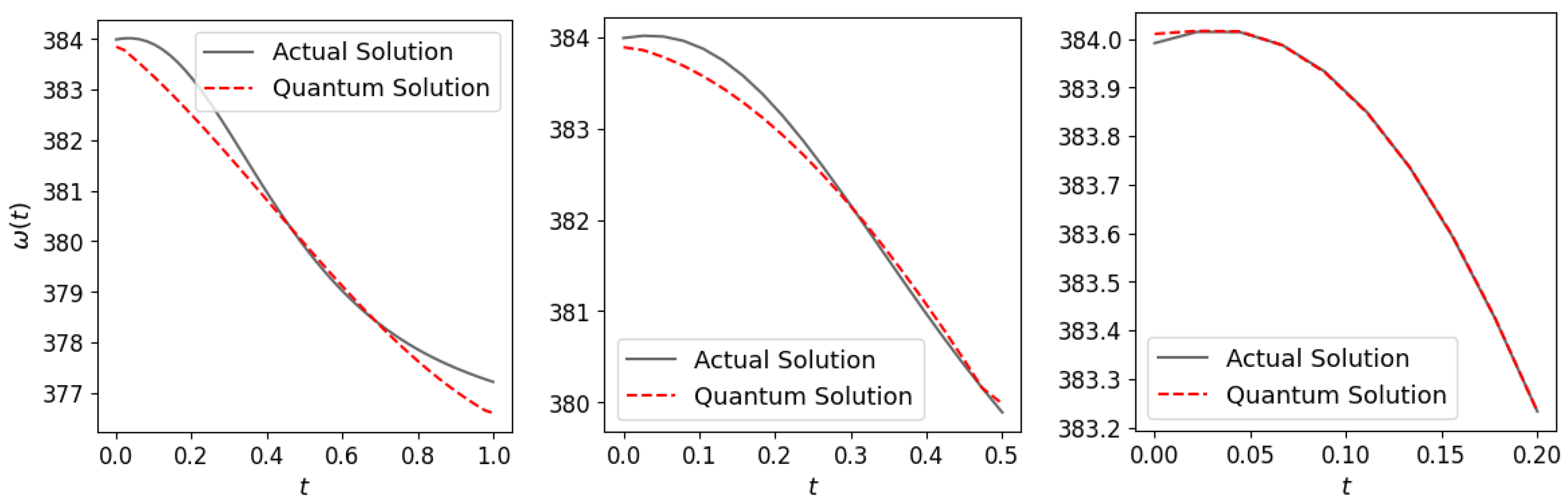
Figure 8 demonstrates the effect of different time spans on the solution accuracy for
in the one-machine system using 20 training points. The results indicate that a time span of
s delivered the most precise outcomes. However, a span of
s also provided satisfactory results, and to minimize the number of computational runs, we selected
s. Following similar experimental guidance, a span of
s was chosen for the three-machine DAEs, balancing precision and computational demand.
5.3. Number of Training Points
The number of training points for a quantum circuit is determined by balancing accuracy against computational constraints. Increasing the number of points typically improves precision but also requires more computational time. Hence, optimizing the number of training points involves striking a balance between computational efficiency and desired accuracy.
Figure 9 illustrates this relationship for the SMIB system, showing how an increased number of training points reduces the error between the quantum approximation and the actual solution for
over the interval
.
5.4. Complete Simulation
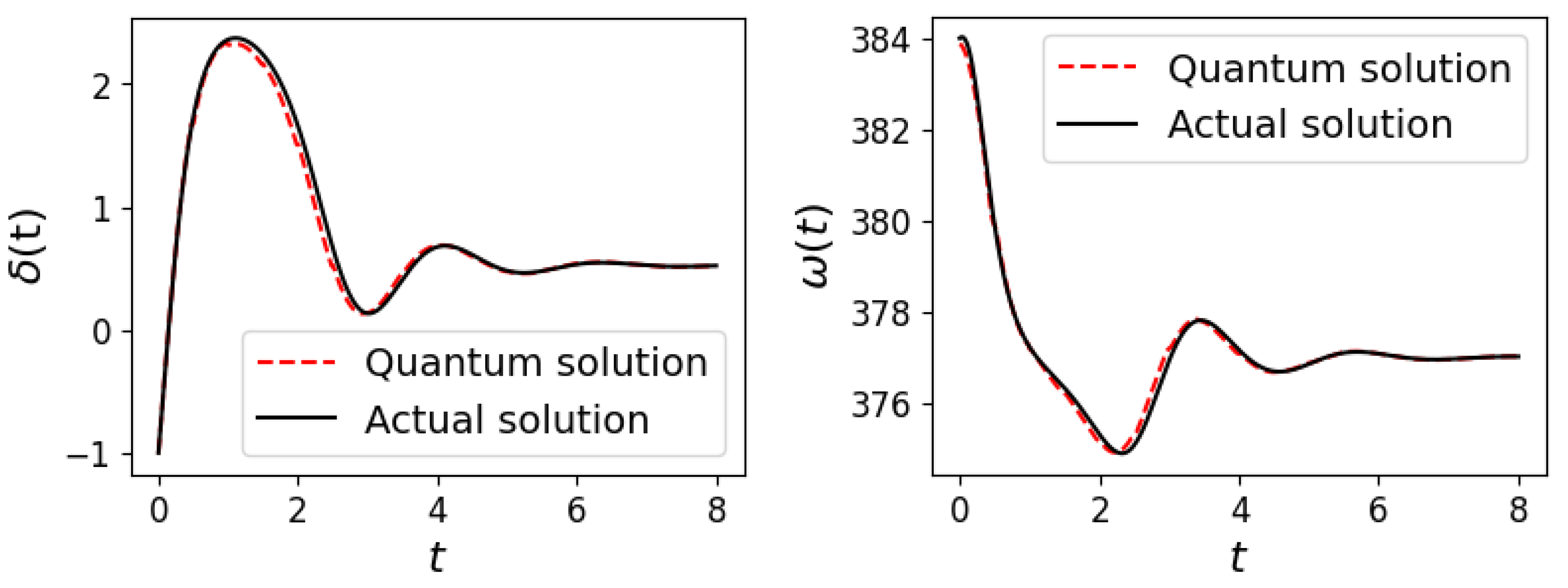
By aggregating results over various time intervals, we successfully solved the DAEs for both one-machine and three-machine systems. In the one-machine scenario, we set the time span to 8 s with a time interval of
s, using 20 training points per interval. We utilized the SFQ structure with
embedding, and the complete solution is presented in
Figure 10.
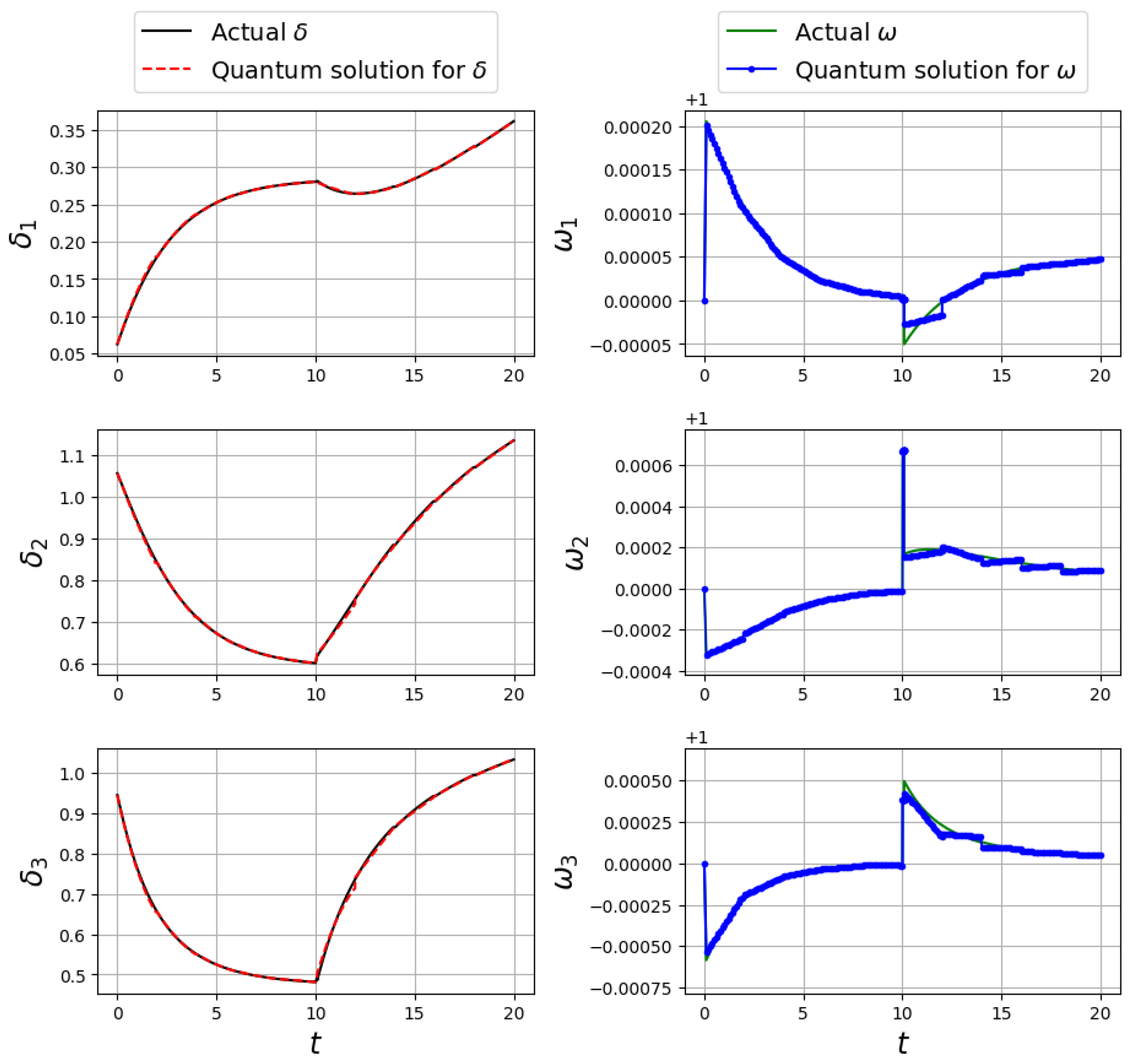
For the three-machine system, we set the time span to 20 s, maintaining a time interval of
s, and similarly using 20 training points per interval. The complete solution achieved with the PFQ structure is illustrated in
Figure 11.
The results affirmed that the quantum solutions closely aligned with the actual solutions for both and variables, demonstrating the ability of the SFQ and PFQ to accurately simulate the dynamics of power systems in the one-machine and three-machine cases, respectively.


