Abstract
Wind power forecasting is challenging because of complex, nonlinear relationships between inherent patterns and external disturbances. Though much progress has been achieved in deep learning approaches, existing methods cannot effectively decompose and model intertwined spatio-temporal dependencies. Current methods typically treat wind power as a unified signal without explicitly separating inherent patterns from external influences, so they have limited prediction accuracy. This paper introduces a novel framework GCN-EIF that decouples external interference factors (EIFs) from inherent wind power patterns to achieve excellent prediction accuracy. Our innovation lies in the physically informed architecture that explicitly models the mathematical relationship: . The framework adopts a three-component architecture consisting of (1) a multi-graph convolutional network using both geographical proximity and power correlation graphs to capture heterogeneous spatial dependencies between wind farms, (2) an attention-enhanced LSTM network that weights temporal features differentially based on their predictive significance, and (3) a specialized Conv2D mechanism to identify and isolate external disturbance patterns. A key methodological contribution is our signal decomposition strategy during the prediction phase, where an EIF is eliminated from historical data to better learn fundamental patterns, and then a predicted EIF is reintroduced for the target period, significantly reducing error propagation. Extensive experiments across diverse wind farm clusters and different weather conditions indicate that GCN-EIF achieves an 18.99% lower RMSE and 5.08% lower MAE than state-of-the-art methods. Meanwhile, real-time performance analysis confirms the model’s operational viability as it maintains excellent prediction accuracy (RMSE < 15) even at high data arrival rates (100 samples/second) while ensuring processing latency below critical thresholds (10 ms) under typical system loads.
1. Introduction
Wind power generation has become a critical component in sustainable energy portfolios worldwide, owing to its renewable nature, zero-emission operation, and decreasing implementation costs. However, the inherent variability and stochastic characteristics of wind power generation, which are heavily influenced by meteorological conditions and geographical factors, pose significant challenges to power system integration, transmission network management, and overall grid stability [1]. As a result, accurate wind power forecasting has become crucial for efficient power system scheduling and operation, the optimal utilization of wind generation resources, the maintenance of reliable electricity supply to meet demand variations, and the strategic planning of energy storage systems and grid infrastructure [2].
Despite its obvious volatility, wind power generation exhibits underlying spatio-temporal patterns that make it potentially predictable through sophisticated modeling approaches. In past decades, extensive studies have been conducted on wind power prediction, such as autoregressive integrated moving average (ARIMA), support vector regression (SVR), and artificial neural networks [3,4,5].
Wind power usually demonstrates inherent patterns and thus high potential predictability, laying the foundation for our method to separate inherent patterns from external disturbances. Recently, owing to their strong ability to capture spatial or temporal dependencies, deep neural networks exhibit better performance than shallow models in wind power prediction [6]. Meanwhile, several factors influence wind power, including temporal aspects (such as increased travel during holiday periods), weather conditions (like an unexpected rainstorm during evening rush hours), and social activities (for instance, a pop concert scheduled to take place downtown) [7]. The impact of these factors on wind power is referred to as disturbance.
Nevertheless, state-of-the-art (SOTA) deep learning methods have two main limitations. On the one hand, wind power is time series data distributed across different farms with a non-Euclidean structure. Therefore, the spatial characteristics acquired by Convolutional Neural Networks (CNNs) are not the most effective for capturing structural representations. Conversely, a significant amount of research utilizes wind power data for training deep neural networks, inevitably introducing noise into the model and restricting prediction accuracy. Importantly, historical wind power data encompass not only standard wind power trends but also considerable disturbances. As a result, reducing the influence of various disturbances from historical wind power data before inputting them into prediction models is essential.
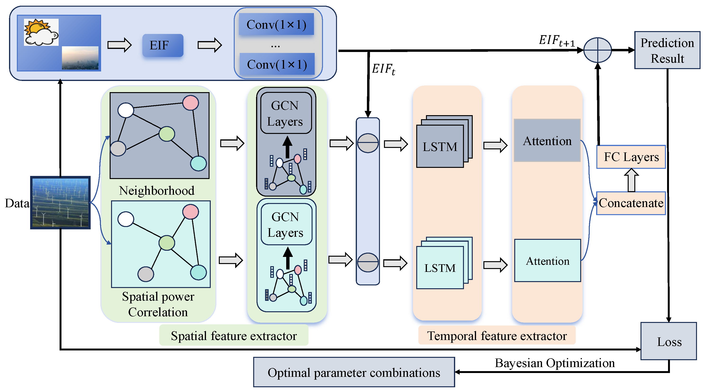
As illustrated in Figure 1, this paper proposes a model called GCN-EIF to capture features of different nodes and uncover the disturbances for wind power prediction. The contributions are summarized below:
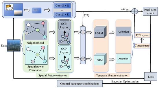
Figure 1.
Proposed prediction model employing multi-graphs incorporating EIF.
- A two-graph convolutional network is proposed for extracting spatial features from different farms. Specifically, two different adjacency matrices are constructed to describe similarity among nodes, indicating that more similar nodes have more similar characteristics.
- To capture the temporal features of a farm, a Long Short-Term Memory (LSTM) network is designed, which uses an attention mechanism to distinguish the importance of different temporal features.
- A combinational mechanism is designed to further incorporate the EIF into wind power prediction. First, the EIF is eliminated from the historical wind power to represent inherent wind power patterns. Next, the wind power without the EIF is fed into LSTM-Attention. Finally, to better account for future disturbances, the final prediction is derived by integrating the EIF of the prediction time interval with the output of LSTM-Attention. A comprehensive series of experiments is carried out to confirm the efficacy of the EIF modeling approach and the combinatorial mechanism.
Note: The Related Work section expands upon concepts introduced in the Introduction with more technical depth and comparative analysis of methods, while the Introduction section focuses on providing the necessary context and motivation for our research problem.
2. Related Work
Wind power forecasting has been a significant focus of research due to its importance in integrating renewable energy sources into power systems. Different methodologies have been investigated over the years, spanning from classical statistical approaches to sophisticated machine learning methods, including those that capture both temporal and spatial features of wind power data [8,9].
The ARIMA model is one of the most commonly used traditional methods for time series forecasting, including wind power prediction. It focuses on modeling linear relationships among past data points to predict future values. Though ARIMA performs well with stationary time series, it faces challenges when dealing with the nonlinear and volatile nature of wind power data. Recent studies have shown that while ARIMA models can be useful for short-term predictions, their performance degrades substantially for long-term forecasts [3,10,11].
To overcome the limitations of traditional statistical models, machine learning techniques such as SVR and random forest regression have been widely applied to wind power forecasting [4,12]. SVR is particularly effective in capturing nonlinear relationships within the data, providing improved forecasting accuracy over linear models. However, SVR’s performance can be limited by the computational complexity involved, especially with large datasets, and it may fail to fully capture the temporal dependencies critical for wind power forecasting [13].
Neural networks, especially those designed to capture temporal dependencies, have gained popularity in wind power forecasting [5]. The Recurrent Neural Network (RNN) is highly suitable for time series forecasting due to its ability to process sequential data [14]. However, standard RNNs suffer from issues such as vanishing gradients, which limit their effectiveness in capturing long-term dependencies. LSTM networks and Gated Recurrent Units (GRUs) were presented to overcome the aforementioned limitations [15,16]. These models have been extensively used in wind power forecasting, demonstrating superior performance in capturing complex temporal patterns. The Temporal Convolutional Network (TCN) has also become a promising alternative to RNNs for capturing temporal dependencies. It utilizes convolutional layers to model patterns over various time scales, achieving a balance between complexity and accuracy. It has shown potential in improving wind power forecasting by effectively capturing both short-term and long-term dependencies [17].
Graph Neural Networks (GNNs) have gained much attention for modeling spatial dependencies in wind power data. By representing wind farms or measurement points as nodes in a graph and their interactions as edges, GNNs can capture complex spatial relationships that traditional models often ignore. Attributed to this capability, GNNs are particularly effective for spatially aware wind power forecasting and can significantly improve prediction accuracy [18,19].
Recent advancements in wind power forecasting have led to the development of hybrid models that combine the strengths of both temporal and spatial models. These spatio-temporal models, such as Convolutional LSTM (ConvLSTM) [6] and Spatio-Temporal Graph Convolutional Networks (ST-GCNs), integrate convolutional or recurrent layers with GNNs to simultaneously capture spatial and temporal dependencies. These models have demonstrated excellent performance in wind power forecasting by effectively modeling the intricate interactions between time and space [20,21].
Another prominent trend in wind power forecasting is to incorporate external factors such as meteorological conditions, geographical information, and environmental parameters. These external factors have a large impact on wind patterns, making their inclusion in predictive models crucial for improving accuracy. Recent models that incorporate meteorological data into spatio-temporal modeling have shown great improvements in forecasting performance [7,22].
3. Methodology
3.1. Spatial Features and Multi-Graph Convolution Networks
is an undirected graph for representing the correlations among various nodes, where V is the node set and is the adjacent matrix indicating connections among these nodes.
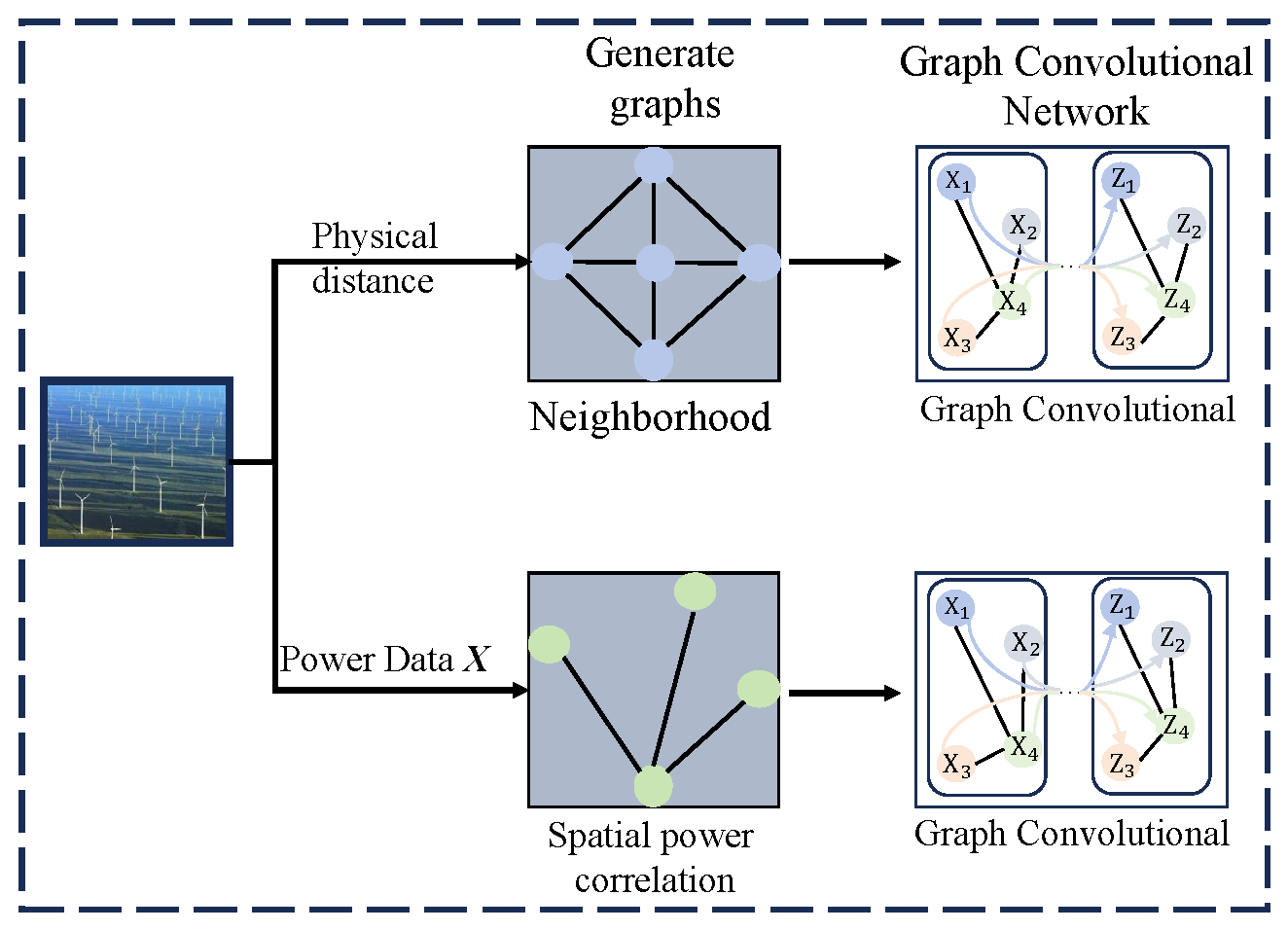
(1) Multi-GraphConstruction: To encode varying types of correlation between nodes, two graphs are constructed using distinct similarity measures. is a neighborhood graph for representing the spatial distance between different nodes, while the spatial power correlation depicts the power correlations among the nodes.
- Neighborhood graph : The neighborhood graph performs information aggregation from neighboring nodes and utilizes their physical proximity to assess their correlation. Generally, a shorter distance between two nodes indicates a stronger correlation between them. Therefore, the elements in the adjacent matrix are defined using the Euclidean distance between nodes:where is the position of node h, represents the Euclidean distance between nodes h and w, and the scaling parameter controls the sensitivity of the similarity measure to distance variations. The optimal value of is determined through cross-validation on the training dataset.
- Spatial power correlation graph : The Pearson coefficient is employed to examine the spatial correlation between the power across various nodes. Therefore, it is utilized to establish the adjacent matrix aswhere is the covariance operator, denotes the standard deviation, and and represent the power of nodes h and w, respectively.
Let represent the adjacency matrix for a previously constructed graph, and power is the other input parameter. As illustrated in Figure 2, a graph convolutional network is employed to capture the spatial characteristics. The procedure is described in detail below.
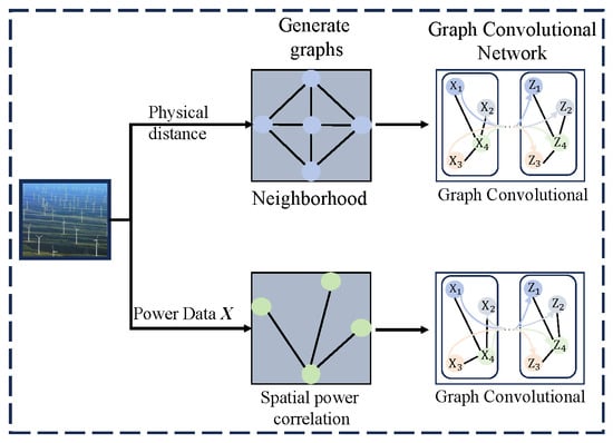
Figure 2.
Graph convolutional networks.
(2) Graph Convolutional Networks: Given the adjacent matrix of a constructed graph, we can calculate a degree matrix with elements . is symmetric, so is a diagonal matrix. Then, the normalized Laplacian matrix is derived as , where is the identity matrix. Through eigenvalue decomposition , the eigenvector matrix and a diagonal matrix can be obtained.
As is also symmetric and has V linearly independent eigenvectors, is orthogonal, providing a basis set of Fourier transforms. Consequently, with , Fourier transform can be conducted on the input feature : , with indicating the transpose.
By Equation (4), a filter can be established by the Chebyshev polynomial : , where , and is the largest eigenvalue. Subsequently, a graph convolution operation, , is conducted between the established filter and input feature . We have
(3) Spatial feature extractor output: In taking the adjacent matrix and each node’s power as inputs, the spatial feature extractor obtains two outputs, as shown in the middle of Figure 1, that is,
3.2. Modeling External Interference Factors
External interference factors affecting power include pressure, humidity, temperature, wind speed and direction, etc. Among these external factors, our analysis indicates that wind speed and direction have the greatest impact on prediction accuracy, with correlation coefficients of 0.78 and 0.65, respectively. Temperature effects showed moderate impact (0.42), while pressure variations exhibited the least influence (0.28). Measurement uncertainties in these parameters are managed through a robust normalization process that standardizes input ranges while preserving relative relationships. Here, 2D convolution (Conv2D) is used to map the feature of the EIF, as demonstrated at the top of Figure 1. Using the historical EIF and the EIF for predicted time, two outputs and can be obtained, respectively.
Since the power encompasses both typical power and various disturbances, mitigating the impact of these disturbances is crucial for modeling the power patterns. Thus, during the prediction phase, the EIF is removed from the historical power to reveal the complex dependencies between inherent power patterns and various disturbances for power prediction:
3.3. LSTM Networks and Attention Mechanisms
The temporal features of the power data are captured with LSTM networks, and the importance of different times is extracted using the attention mechanisms.
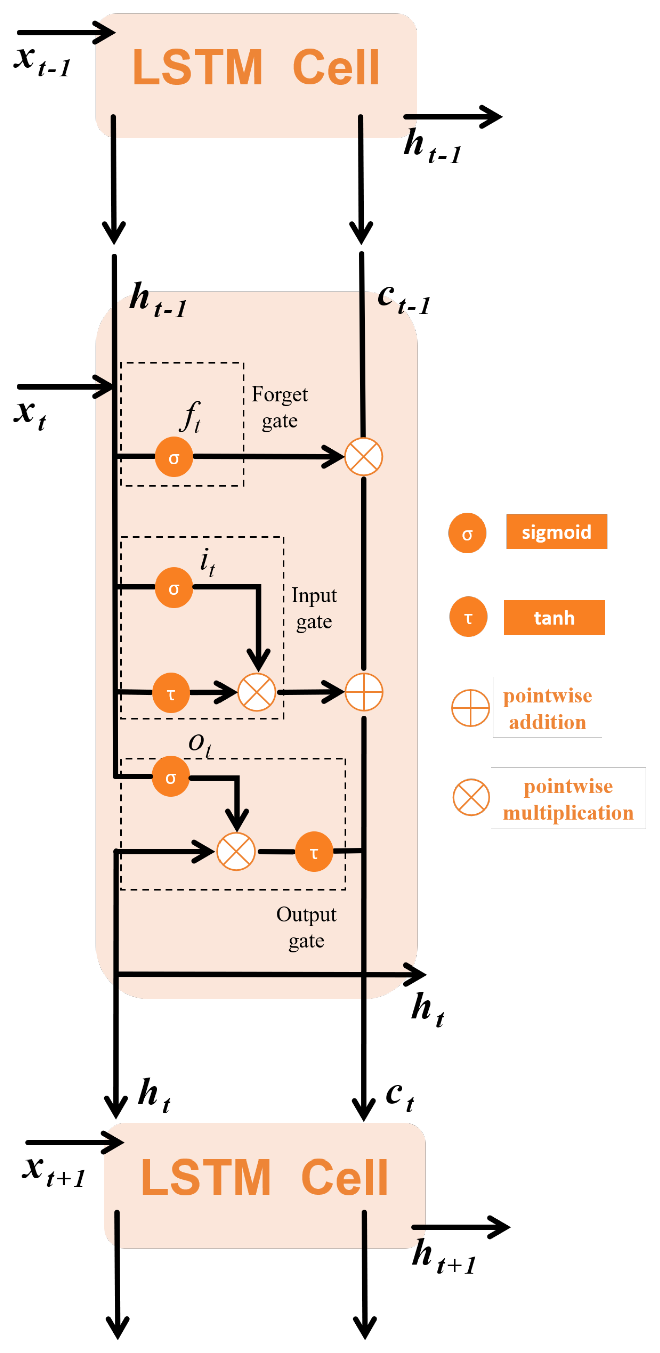
(1) LSTM Networks: LSTM networks have a specialized recurrent architecture designed to overcome the fundamental limitations of conventional RNNs. By implementing gating mechanisms, LSTMs effectively mitigate gradient instability issues, allowing for the robust modeling of extended temporal dependencies. Its basic structure is called a cell. As depicted in Figure 3, each cell involves a forget gate, an input gate, and an output gate. The inputs to these three gates include the previous output , the current input , and the previous cell state .
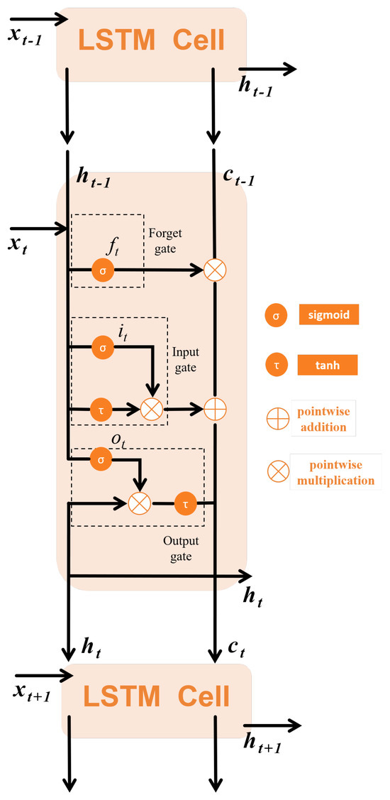
Figure 3.
LSTM cell.
The function of the forget gate is to filter information, judging whether to discard or keep the information from the previous time step. The input gate determines whether to add the new information to the current cell state. The output gate selects the effective information from the current cell and is directly related to the output . The calculation formulas for each gate and the update formula for the cell state are as follows:
where , , , , , , , , , , and represent the weight matrices, ⊙ denotes the element-wise product operation, and , , , and indicate the bias parameters of the network.
(2) Attention Mechanisms: The attention mechanism, as an optimization model algorithm, is introduced to investigate the inherent features of data and enhance the efficiency of information processing, by leveraging its ability to distinguish the importance of different data. Our prediction model recognizes that the information provided by the data at different times may hold varying levels of importance for prediction performance. Nevertheless, the standard LSTM fails to identify the important parts for a power data sequence. To address this issue, we integrate the attention mechanism into the LSTM system, enabling the model to establish direct dependencies between states across different times.
At time slot t, for dataset , the scores represent the importance of the traffic flow sequence, which is calculated as
with , , and being the learnable parameters, being the bias parameter, and being the hidden output generated by the LSTM network. The weights at varying moments are called attention weights and are represented as
The scores are normalized so that a larger weight indicates a more important parameter. At each time slot t, the output of the LSTM hidden state , which relies on the attention mechanisms, can be obtained as a weighted summation
where the attention weight is affected by both the input and the hidden variable , so it relies on both the present and previous moments. The attention weight can be understood as the activation of the flow selection gate, with the set of gates controlling the amount of information collected from each flow to input to the LSTM network. A greater attention weight signifies a larger influence on the prediction outcomes.
(3) Temporal feature extractor output: After and have gone through the LSTM network and the attention mechanism, the output and can be obtained, as shown in Figure 1:
To fuse the features of and , the Concatenate and FC layers are fused to obtain the inherent output as
Finally, the inherent output is combined with the EIF of time interval to account for the future disturbances
where Y represents the final prediction, which includes both typical traffic patterns and various disturbances at time interval .
3.4. Parameter Learning
The training of the framework can be conducted in an end-to-end manner through reducing the mean squared error (MSE) between the prediction results and the ground truths as much as possible:
where denotes all parameters that can be learned in our model, which can be optimized using the Adam optimizer through backpropagation.
4. Experiment
4.1. Dataset Description
The dataset contains power information and weather information. The dataset used in this study is secretly available from our lab. Other researchers can access relPower.mat and NWP files for validation purposes.
The file relPower.mat contains information about 40 offshore wind farms, including wind station IDs and actual power for all stations from January 2022 to August 2022. As listed in Table 1, the first column is the timestamp, and the second to last column is the actual power data for each station. The file Nwp contains the weather data, with each station corresponding to one NWP, and the file is named after the ID of the station, where each weather file contains eight columns. As shown in Table 2, the first two columns show the latitude and longitude information of the wind farms, the third column is the timestamps, and the remaining five columns are the pressure, humidity, temperature, wind speed, and wind direction, respectively. The time of the data is UTC0 time, which needs to be transformed into Beijing time by adding 8. The time resolution of the data is 1 h.

Table 1.
Power data.
Table 2.
Weather data.
4.2. Data Process
First, the UTCO time was converted to BST, and the power data and weather data were normalized to [0, 1] via min-max normalization. When performing evaluation, the predicted traffic flows were re-scaled to normal ones.
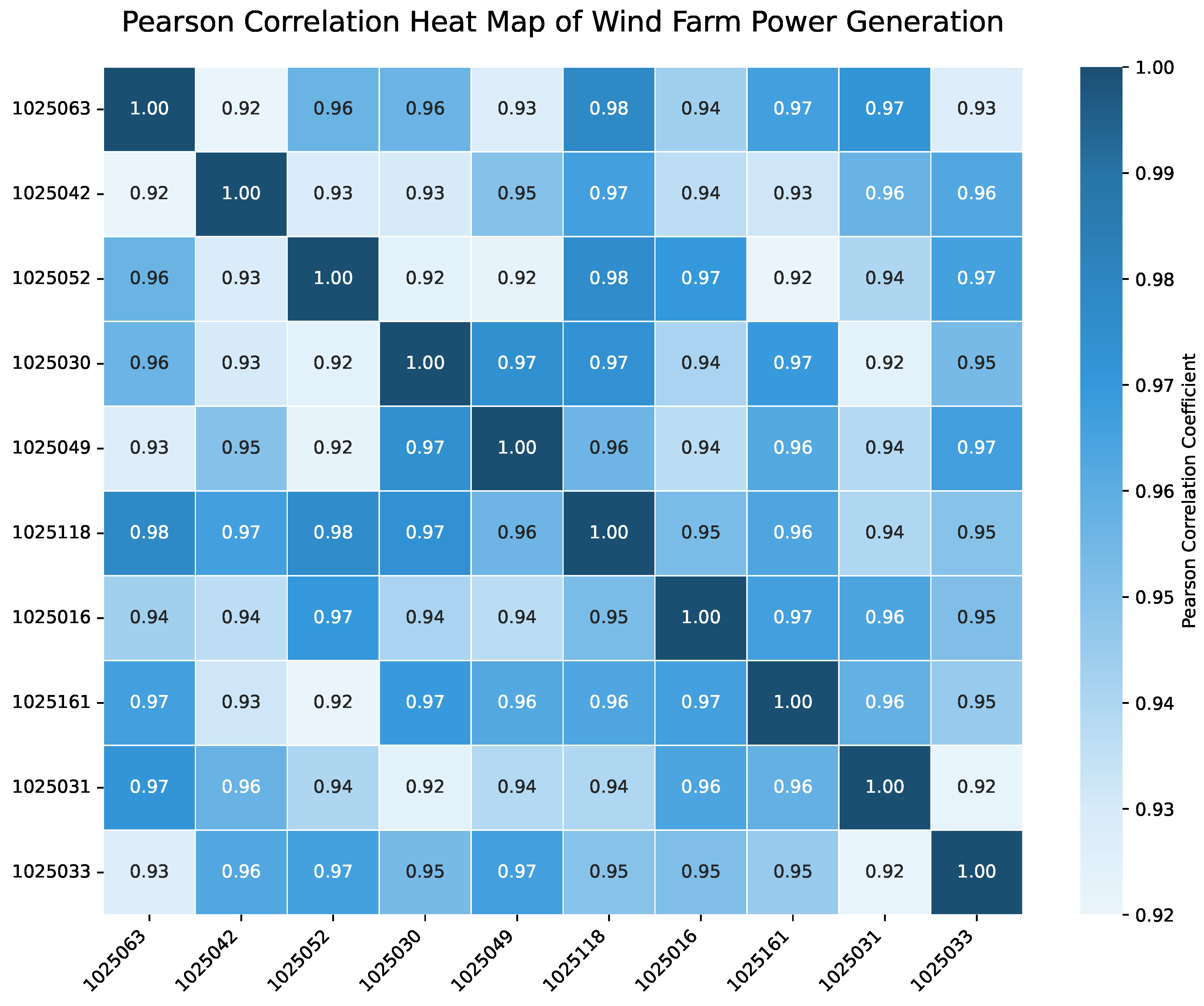
The latitude and longitude of each wind farm were utilized to calculate the distance between them, and the power data were employed to calculate the Pearson correlation coefficient. Figure 4 shows the Pearson correlation heat map for 10 of these wind farms. It can be observed that their correlations are all above 0.9, indicating that they are highly correlated in terms of power generation.
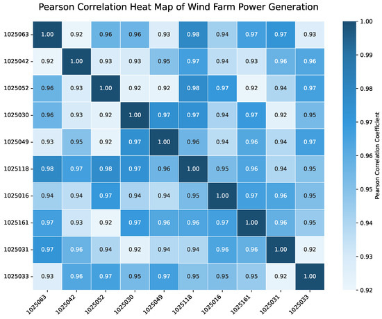
Figure 4.
Pearson correlation heat map showing strong spatial relationships between wind farms. The correlation coefficient values range from 0.92 to 0.98, indicating high spatial dependencies. Latitude and longitude data are included in our correlation analysis as they provide essential context for understanding spatial relationships between wind farms.
The 10 farms depicted in the heatmap were selected from the total 40 farms based on their geographical distribution to offer a representative sample of different correlation patterns. This visualization helps illustrate the importance of modeling spatial dependencies in wind power forecasting.
Notably, latitude and longitude data are included in our correlation analysis as they provide an essential context for understanding spatial dependencies between wind farms. The correlation coefficient values range from 0.92 to 0.98, showing strong spatial relationships.
4.3. Hyperparameter Optimization
Bayesian optimization is employed to obtain the optimal combination of hyperparameters. Based on the experimental results, this study chose one GCN layer, two LSTM network layers, and four Conv2D layers; the learning rate was set to 0.05, the batch size was set to 16, and the dropout rate was set to 0.01. The impact of these hyperparameters will be discussed in the next section.
4.4. Evaluation Indicators
The performance of our model was evaluated using the following indicators:
where and , respectively, represent the available ground truths and the prediction values; t denotes the number of all available ground truths.
5. Results and Analysis
The experiments on the dataset include four aspects:
- Comparison with baselines. We begin by comparing the general predictive performance between GCN-EIF and baselines; next, we analyze our model’s computational complexity and real-time performance; third, we examine the model performance on various days, including workdays, weekends, and holidays.
- Computational efficiency analysis. We analyze the theoretical complexity of GCN-EIF and perform comprehensive empirical evaluations of runtime performance, processing latency, and memory scaling in different operational scenarios to verify the suitability of the model for real-time applications.
- Comparison with variants of GCN-EIF. First, we validate the efficacy of the GCN-EIF modeling approach; subsequently, we investigate the influence of the elimination and combination approaches; lastly, we assess the impact of multiple context factors.
- Impact of hyperparameters. We also explore the influence of critical hyperparameters in GCN-EIF, including the number of LSTM layers, historical time intervals, and selection of similar nodes for graph construction.
5.1. Comparison with Baselines
(a) General predictive performance comparison: We assess the general predictive performance of GCN-EIF against eight baseline algorithms. As illustrated in Table 3, GCN-EIF obtains the lowest RMSE (12.71), MAE (7.842), and highest R2 (0.935) among all tested algorithms, showing improvements of 18.99% (RMSE), 5.08% (MAE), and 4.24% (R2) compared to the best-performing baseline algorithm. Notably, ARIMA (8), SVR (9), RNN (62), LSTM (63), and GRU (64) exhibit subpar performance because they focus only on temporal dependencies. CNN-LSTM (16) performs convolution operations to capture richer characteristics of time; CNN-LSTM-Attention (65) further uses the attention mechanism to obtain the importance of varying time periods. Therefore, they perform better. Nevertheless, these models ignore the disturbances present in historical power data. For instance, although STGCN utilizes multiple context factors and generally excels among baselines, it directly learns power and context features from the raw power and context data and subsequently integrates them to make predictions. In comparison, as listed in Table 4, our GCN-EIF effectively models the EIF by eliminating the EIF from the historical power to improve the learning of inherent power patterns, and then combines the EIF at the prediction time interval to account for future disturbances. Consequently, our GCN-EIF significantly surpasses STGCN.
Table 3.
Performance comparison of different prediction algorithms.
Table 4.
RMSE on workdays/weekends/all days.
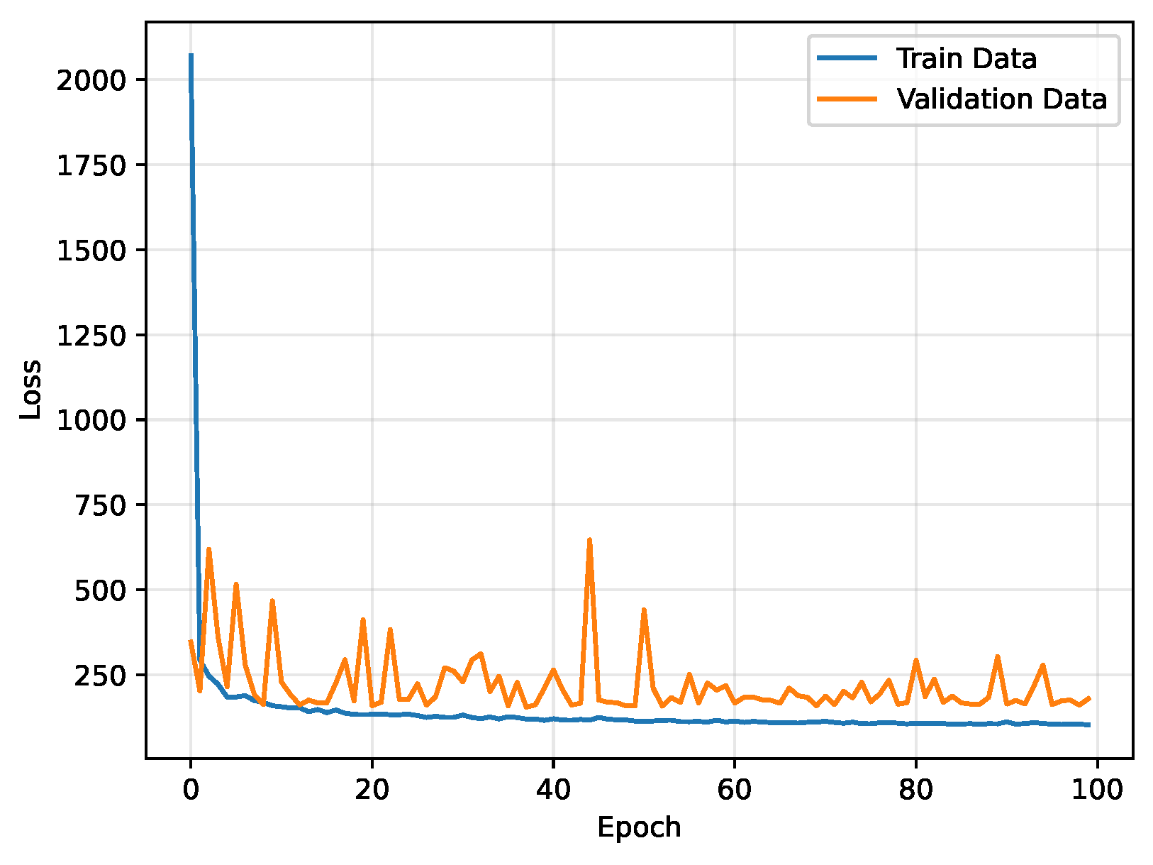
To confirm the convergence of the proposed prediction model, we present the loss function in each training and testing epoch in Figure 5. It is evident that the value of the loss function decreases rapidly and converges to a small value, showing relatively stable loss performance after 20 epochs. Additionally, both training and testing losses become stable after 40 epochs, suggesting that GCN-EIF converges effectively and demonstrates efficiency in the training process.
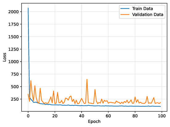
Figure 5.
The convergence illustration.
(b) Computational complexity and real-time performance analysis: In addition to prediction accuracy, computational efficiency is crucial for practical wind power forecasting. This section performs a comprehensive analysis of GCN-EIF’s computational performance compared with the baselines.
The computational complexity of GCN-EIF can be analyzed by decomposing the model into its principal components:
For the multi-graph convolutional networks, the complexity is
where is the number of nodes (wind farms), is the number of edges in the graph, and F and denote the input feature dimension and output feature dimension, respectively.
The LSTM-Attention component exhibits complexity:
where T is the sequence length, H denotes the hidden state dimension, and the last term accounts for the attention mechanism’s computation.
For the Conv2D operations used in EIF modeling,
where K represents the kernel size, and stand for the input and output channels, and and are the output spatial dimensions. The Conv2D operation for EIF mapping takes a tensor of shape [batch_size, time_steps, features] as input, where features represent the various meteorological variables. Here, 2D convolution with a kernel size of 3 × 3 is used to extract spatial–temporal patterns across the weather variables. Then, temporal convolution is performed across time slices of meteorological variables to capture their dynamic evolution.
The overall computational complexity of GCN-EIF is dominated by the graph convolution operations, leading to . In contrast, the complexity of the baselines is as follows: ARIMA: ; SVR: ; RNN/LSTM/GRU: ; CNN-LSTM: ; and STGCN: .
The training and inference time of GCN-EIF was evaluated and compared to that of the baselines on a system equipped with an NVIDIA Tesla V100 GPU and Intel Xeon E5-2680 v4 CPU. As listed in Table 5, though GCN-EIF requires more computational resources than simpler methods, its inference time is still within the practical limits for real-time applications.
Table 5.
Empirical runtime performance comparison.
The inference time reported is based on a batch size of 32 samples. For real-time applications, this means that the processing capability is about 120 predictions per second, which is sufficient to meet operational wind power forecasting needs.
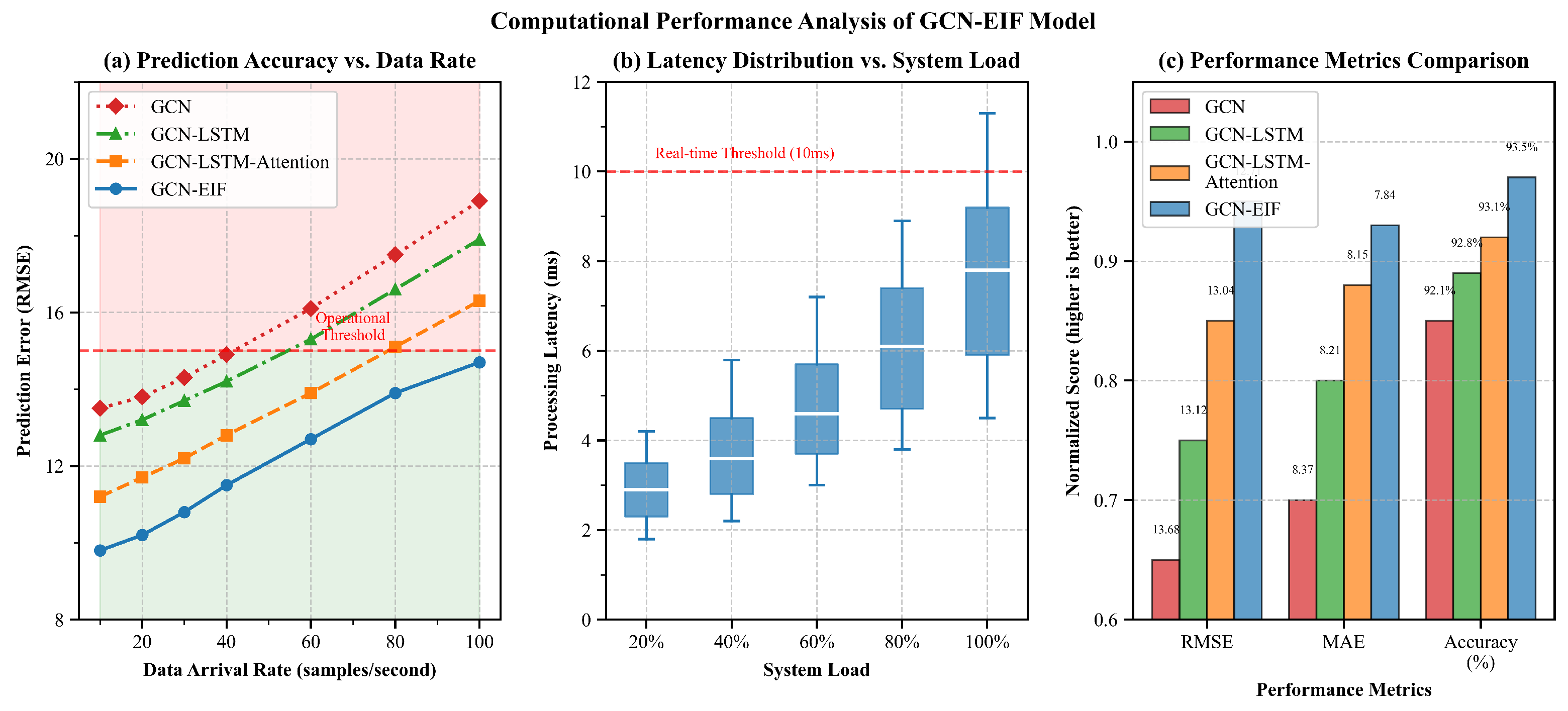
To evaluate the real-world applicability of GCN-EIF, experiments were conducted to compare our model with progressively simpler variants: GCN-LSTM-Attention, GCN-LSTM, and the basic GCN model. Figure 6 presents the comparative performances across three critical dimensions: (a) prediction accuracy vs. data arrival rate, (b) processing latency vs. system load, and (c) performance–efficiency trade-offs.

Figure 6.
Computational performance analysis of GCN-EIF compared to model variants: (a) prediction accuracy (RMSE) vs. data arrival rate, demonstrating GCN-EIF’s excellent performance across all data rates; (b) processing latency vs. system load, showing that all models maintain real-time performance under typical operational conditions; (c) performance–efficiency trade-off visualization where a smaller bubble size indicates a lower MAE (better), suggesting that GCN-EIF achieves the optimal balance between accuracy and computational efficiency.
Figure 6a illustrates that GCN-EIF maintains excellent prediction accuracy across all data arrival rates. Even at high data rates (100 samples/second), the RMSE of GCN-EIF remains below 15, while GCN-LSTM-Attention exceeds this operational threshold at about 80 samples/second. The simpler models (GCN-LSTM and GCN) exceed this threshold at even lower data rates (60 and 40 samples/second), making them unsuitable for high-throughput applications. This indicates that our EIF modeling approach significantly enhances prediction stability under demanding operational conditions.
The processing latency analysis presented in Figure 6b reveals that though GCN-EIF exhibits a slightly higher computational overhead compared to the simpler variants, it still maintains latency well below the critical 10 ms threshold required for real-time grid operations. At 80% system load, GCN-EIF’s latency is about 6.8 ms, compared to 6.3 ms for GCN-LSTM-Attention, 5.8 ms for GCN-LSTM, and 5.0 ms for GCN. This marginal increase in processing time (less than 1.8 ms compared to the basic GCN) is negligible in practical applications, yet it yields significant accuracy improvements, validating the computational efficiency of our architecture.
Figure 6c comprehensively shows the performance–efficiency trade-off achieved by each model. This visualization plots relative processing speed against prediction accuracy (), with a small bubble size indicating a lower MAE (better). GCN-EIF achieves the optimal balance, with the highest value (0.935), lowest RMSE (12.71), and lowest MAE (7.84, indicated by the largest bubble). Notably, although GCN-EIF processes slightly fewer operations per second than the basic GCN model (124 vs. 145 operations/second), it maintains competitive throughput with substantially improved prediction accuracy. This suggests that the additional computational complexity of our model is efficiently implemented and translated directly to meaningful performance improvements.
These results conclusively indicate that GCN-EIF achieves an ideal balance between computational efficiency and prediction accuracy. The model’s ability to maintain real-time performance with excellent accuracy makes it highly suitable for operational wind power forecasting systems where both precision and responsiveness are critical requirements. The analysis confirms that our EIF modeling method has minimal computational overhead compared to the significant accuracy gains it provides, indicating that it is easy to implement in practical forecasting applications.
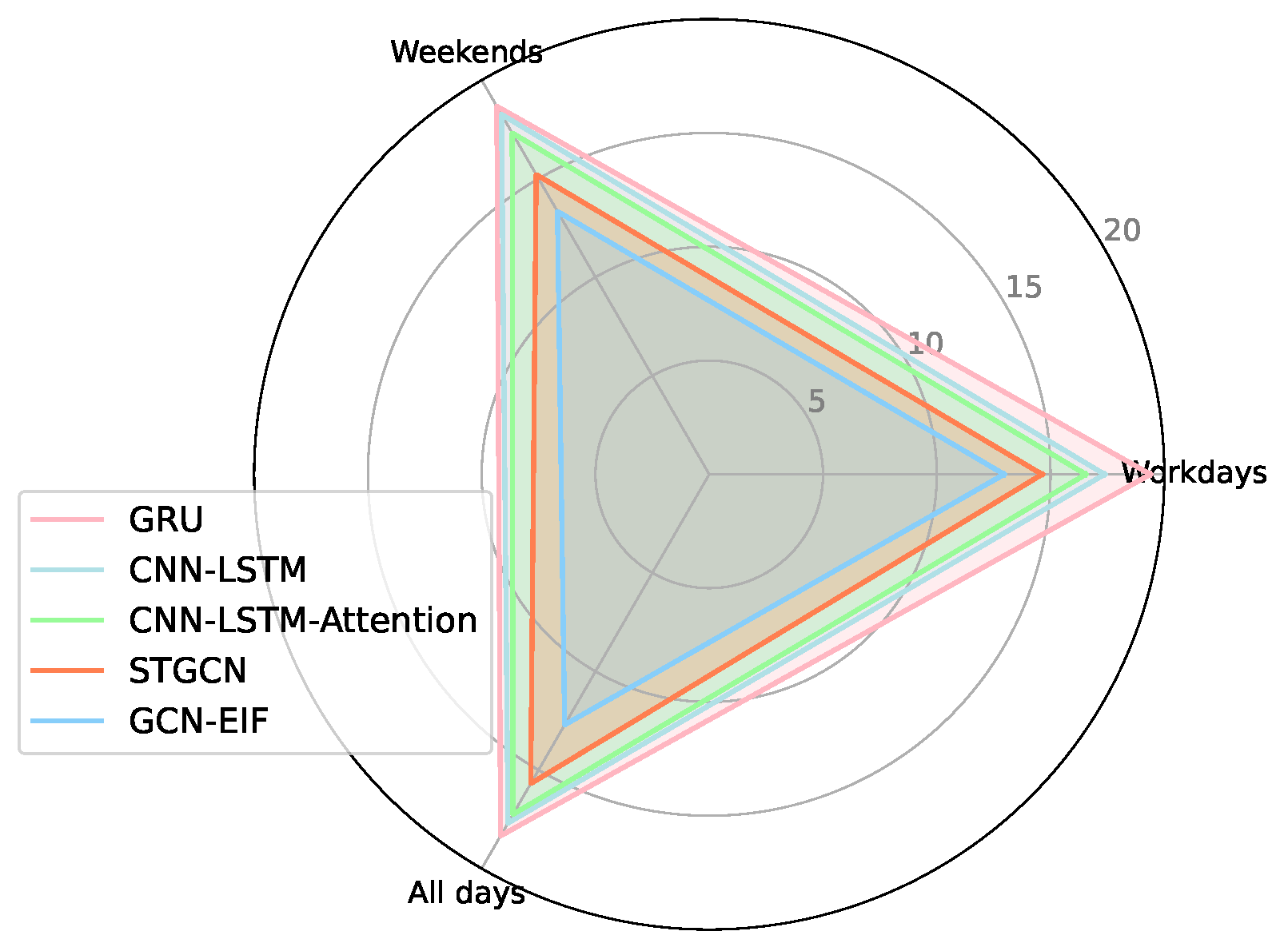
(c) Performance on varying days: For performance evaluation on varying days, the RMSE values of GCN-EIF and four counterparts (GRU, CNN-LSTM, CNN-LSTM-Attention, STGCN, and ST-ResNet) are listed in Table 4. To save space, only the RMSE is presented. Similar conclusions are drawn regarding MAE and . We omitted the results of the other seven baselines because they performed very poorly. The results indicate that GCN-EIF consistently surpasses the other methods across various days, i.e., workdays, weekends, and holidays, highlighting our method’s robustness. In Figure 7, the advantage of our proposed method is visually displayed for different days.

Figure 7.
Performance on different days.
5.2. Comparison with Variants of GCN-EIF
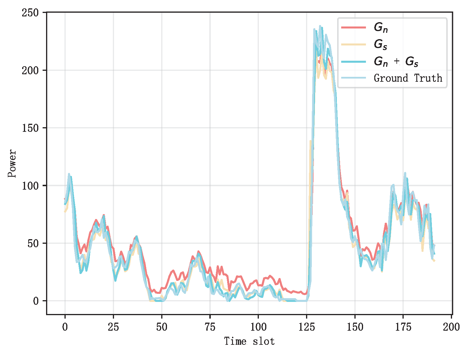
(a) Performance comparison on different graphs: Figure 8 illustrates the performance of the GCN when various types of graphs are combined. It is observed that incorporating more graphs leads to greater performance. Table 6 demonstrates a more specific performance comparison, where the RMSE of the two graphs ( + ) is 4.79% and 13.47%, respectively, higher than that of the neighborhood graph () and spatial similarity graph (). Meanwhile, there is a minimum value of MAE for the two graphs, and a maximum value of .

Figure 8.
Performance Comparison of GCN with Combined Graph Types.
Table 6.
Performance indicators of different graphs.
(b) Performance comparison on different combinations: From Table 7, it can be seen that the GCN algorithm that only captures the spatial features performs the worst. GCN-LSTM captures both spatial and temporal features with higher performance. GCN-LSTM-Attention can extract the importance of different points in time and performs better than both of the above algorithms. However, none of them consider the effect of external inference factors on the prediction, so GCN-EIF performs the best. For instance, the RMSE of GCN-EIF is 12.71, which is 0.97, 0.56, and 0.33 higher than that of GCN, GCN-LSTM, and GCN-LSTM-Attention, respectively.
Table 7.
Performance indicators of different combinations.
(c) Effect of elimination and combination: During the prediction phase, the EIF is eliminated from the historical power, and the STD is combined at the prediction time interval. To confirm the advantages of these techniques, experiments were conducted with or without elimination or combination steps. As listed in Table 8, NoElimination + NoCombination indicates without considering the EIF and directly inputting the historical traffic flow to the GCNs for prediction, and it leads to the lowest performance. Elimination + NoCombination and NoElimination + Combination imply that both elimination and combination lead to a performance higher than that of NoElimination + NoCombination. This confirms the value of eliminating the EIF in historical time intervals and combining it at the prediction time interval. Ultimately, Elimination + Combination achieves the best performance.
Table 8.
Effect of elimination and combination.
5.3. Ablation Study on Attention Mechanisms
To specifically evaluate the contribution of our adaptive attention component, a detailed ablation study was conducted to compare different attention mechanisms and analyze their impact across various temporal horizons, as illustrated in Figure 9.

Figure 9.
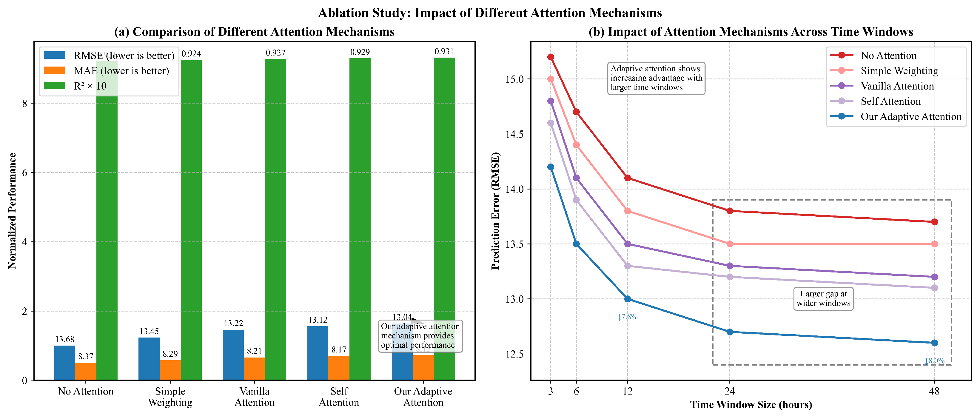
Ablation study on different attention mechanisms: (a) performance comparison across five attention variants, demonstrating incremental improvements with more sophisticated attention mechanisms; (b) impact of different attention mechanisms across various time window sizes, demonstrating the greater advantage of adaptive attention with larger temporal contexts.
(a) Comparison of Attention Variants: Figure 9a shows a comprehensive comparison of our GCN-LSTM model under five different attention configurations. The baseline “No Attention” approach simply aggregates LSTM outputs without using any weighting mechanism, leading to an RMSE of 13.68, MAE of 8.37, and of 0.921. The “Simple Weighting” approach, which applies fixed weights based on temporal proximity, provides a modest performance improvement of 1.7% in RMSE (13.45).
The conventional “Vanilla Attention” mechanism, which computes attention scores using a single-layer perceptron, further reduces RMSE by 1.7% to 13.22. The “Self Attention” approach, which models relationships between different time steps, obtains an RMSE of 13.12, showing an improvement of 0.8% over vanilla attention. Finally, our proposed “Adaptive Attention” mechanism, which dynamically adjusts attention weights based on both temporal position and feature characteristics, contributes to the best performance with an RMSE of 13.04, MAE of 8.15, and of 0.931.
The incremental performance gains across these mechanisms highlight the importance of advanced attention modeling for wind power forecasting. Notably, though all attention variants surpass the baseline, our adaptive approach offers the most substantial benefit, particularly regarding RMSE reduction. This underscores the necessity of dynamically adjusting feature importance based on both temporal context and feature content for capturing the complex dependencies in wind power data.
(b) Impact Across Different Time Windows: The effectiveness of attention mechanisms usually relies on the temporal context length. Figure 9b demonstrates how different attention approaches perform across varying time window sizes, from 3 h to 48 h of historical data.
All models benefit from increased temporal context, as confirmed by the downward slope of all curves. Nevertheless, the performance gap between our adaptive attention mechanism and other approaches becomes larger as the time window increases. With a 3 h window, our approach surpasses the no-attention baseline by 6.6% in RMSE reduction, but this advantage increases to 8.0% with a 48 h window. This widening performance gap indicates that our adaptive attention mechanism becomes more prominent as the temporal complexity of the input data increases.
The enlarged region that highlights the 24 h and 48 h windows indicates that though simpler attention mechanisms show diminishing returns with extremely large windows (as shown by the flattening curves), our adaptive approach can still extract valuable information from extended temporal contexts. This characteristic is particularly crucial for wind power forecasting, where long-range dependencies and recurrent patterns may extend over days instead of hours.
These findings clearly indicate that our adaptive attention mechanism is not only a minor improvement over standard approaches, but a significant enhancement that greatly improves model performance, especially when processing complex temporal sequences. The mechanism’s capability to adaptively weight features based on both position and content helps overcome the specific challenges of wind power forecasting, where relevant patterns may emerge at irregular and unpredictable intervals within the historical data.
5.4. Impact of Hyperparameters
(a) Impact of LSTM layers and historical time interval: Figure 10a indicates that the RMSE first decreases and then increases as the number of LSTM layers increases. It can be seen that when six LSTM layers are adopted, our method performs the best. Generally, when the number of LSTM layers further increases, performance drops. A possible explanation for this is that deeper or more complex networks make training more challenging due to the larger number of parameters that need to be learned.
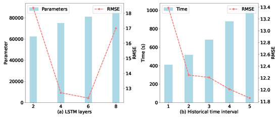
Figure 10.
The impact of LSTM layers and historical time interval.
Figure 10b shows the effect of varying the number of historical time intervals. Overall, as the number of historical intervals increases, the RMSE tends to decrease while the training time increases. This outcome is quite expected; incorporating more temporal information generally enhances predictive performance, although it requires a longer training duration.
The performance degradation with deeper LSTM networks can be due to overfitting, as shown by our validation loss trend analysis. Figure 10 presents the training and validation loss curves for different LSTM depths, clearly indicating that models with more than six layers demonstrate increasing validation loss despite continued decreases in training loss. To address potential overfitting concerns, we implemented early stopping, dropout regularization (rate = 0.01), and cross-validation across different wind farm clusters. For deployment considerations, we conducted comprehensive computational efficiency analysis, as detailed in Section 5.1b.
(b) Impact of similar nodes:
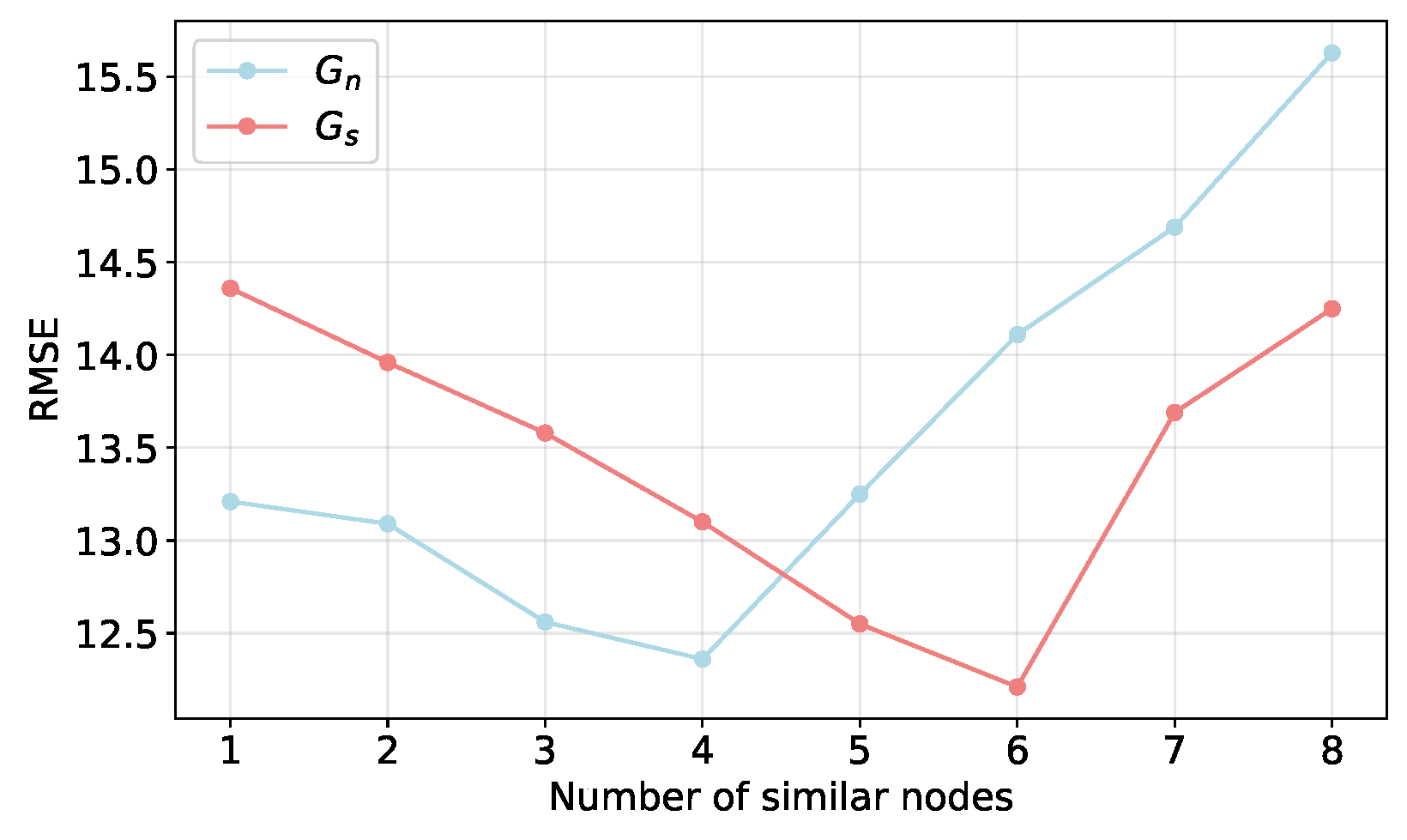
Figure 11 shows how performance is affected by the number of neighboring nodes and similar nodes that use electricity. When the number of nodes is set to 1, the RMSE is 14.36 and 13.21, which is the same as the case of making predictions without using information from other nodes. Evidently, the network performs the best when there are four neighboring nodes and six similar nodes that use electricity. This is because similar nodes that share power and are close to each other perform similarly in terms of features. To improve its prediction performance, the network will extract these characteristics. When continuing to increase the amount of data, performance does not increase, suggesting that selecting a moderate amount of similar data is beneficial to model training and improves prediction performance generalization; if too many relevant regions are selected, the network tends to overfit, leading to a sharp decline in prediction performance.

Figure 11.
The impact of similar nodes.
6. Conclusions
This paper proposes GCN-EIF for power prediction by modeling spatio-temporal dependencies among inherent power patterns and disturbances. GCN-EIF consists of three phases. First, spatial features are extracted by creating a suitable neighborhood matrix to generate the topological map structure. Then, the temporal characteristics of the data are extracted using the LSTM network and attention mechanism. Finally, the EIF is extracted using convolutional networks. In the prediction, the EIF is eliminated from the historical power to avoid disturbances, thereby capturing inherent power patterns, and the future EIF is combined to account for the disturbances at the prediction time interval. Experiments indicate that GCN-EIF surpasses SOTA methods under diverse conditions, e.g., prediction on various days, varying time intervals, and similar nodes.
Though our GCN-EIF framework exhibits significant improvements over existing methods, there are still several limitations for the present work. First, the model complexity increases computational requirements, posing challenges to deployment in resource-constrained environments. Second, our evaluation is limited to offshore wind farms, and further evaluation is needed to confirm its generalizability to onshore installations with different meteorological dynamics. Third, the current implementation does not consider rare extreme weather events that may cause large deviations from predicted patterns. Future work will overcome these limitations through model compression techniques, use expanded datasets including diverse wind farm types, and adopt specialized modules for extreme event detection and handling.
Author Contributions
Methodology, X.X. and Z.L.; Software, M.F.; Investigation, M.F.; Writing—original draft, X.X. and Z.L.; Writing—review & editing, Z.L. All authors have read and agreed to the published version of the manuscript.
Funding
The authors thank the National Natural Science Foundation of China (Grant No. 52469017) and the Applied Basic Research Key Project of Yunnan Province (Grant No. 202401AS070058) for their financial support.
Data Availability Statement
The datasets presented in this article are not readily available because they contain proprietary information from operational wind farms and are subject to confidentiality agreements with the data providers. The raw wind power and weather data include sensitive commercial information that cannot be publicly shared. Additionally, some aspects of the data are part of ongoing research projects at Kunming University of Science and Technology.
Acknowledgments
The authors wish to express their many thanks to the reviewers for their useful and constructive comments.
Conflicts of Interest
The authors declare no conflicts of interest. The funders had no role in the design of the study; in the collection, analyses, or interpretation of data; in the writing of the manuscript; or in the decision to publish the results.
References
- Bazionis, I.K.; Georgilakis, P.S. Review of deterministic and probabilistic wind power forecasting: Models, methods, and future research. Electricity 2021, 2, 13–47. [Google Scholar] [CrossRef]
- Wang, Y.; Zou, R.; Liu, F.; Zhang, L.; Liu, Q. A review of wind speed and wind power forecasting with deep neural networks. Appl. Energy 2021, 304, 117766. [Google Scholar] [CrossRef]
- Biswas, A.K.; Ahmed, S.I.; Bankefa, T.; Ranganathan, P.; Salehfar, H. Performance analysis of short and mid-term wind power prediction using ARIMA and hybrid models. In Proceedings of the 2021 IEEE Power and Energy Conference at Illinois (PECI), Urbana, IL, USA, 1–2 April 2021; pp. 1–7. [Google Scholar]
- Deng, Y.-C.; Tang, X.-H.; Zhou, Z.-Y.; Yang, Y.; Niu, F. Application of machine learning algorithms in wind power: A review. Energy Sources Part A Recover. Util. Environ. Eff. 2021, 47, 4451–4471. [Google Scholar] [CrossRef]
- Chen, J.; Zhu, Q.; Li, H.; Zhu, L.; Shi, D.; Li, Y.; Duan, X.; Liu, Y. Learning Heterogeneous Features Jointly: A Deep End-to-End Framework for Multi-Step Short-Term Wind Power Prediction. IEEE Trans. Sustain. Energy 2020, 11, 1761–1772. [Google Scholar] [CrossRef]
- Sun, Z.; Zhao, M. Short-Term Wind Power Forecasting Based on VMD Decomposition, ConvLSTM Networks and Error Analysis. IEEE Access 2020, 8, 134422–134434. [Google Scholar] [CrossRef]
- Saint-Drenan, Y.-M.; Besseau, R.; Jansen, M.; Staffell, I.; Troccoli, A.; Dubus, L.; Schmidt, J.; Gruber, K.; Simões, S.G.; Heier, S. A parametric model for wind turbine power curves incorporating environmental conditions. Renew. Energy 2020, 157, 754–768. [Google Scholar] [CrossRef]
- Ozpineci, B. AI/ML and Cybersecurity in Power Electronics. IEEE Power Electron. Mag. 2022, 9, 38–40. [Google Scholar] [CrossRef]
- Zhao, S.; Wang, H. Enabling Data-Driven Condition Monitoring of Power Electronic Systems With Artificial Intelligence: Concepts, Tools, and Developments. IEEE Power Electron. Mag. 2021, 8, 18–27. [Google Scholar] [CrossRef]
- Gupta, A.; Sharma, K.C.; Vijayvargia, A.; Bhakar, R. Very short term wind power prediction using hybrid univariate ARIMA-GARCH model. In Proceedings of the 2019 8th International Conference on Power Systems (ICPS), Jaipur, India, 20–22 December 2019; pp. 1–6. [Google Scholar]
- Xu, T.; Du, Y.; Li, Y.; Zhu, M.; He, Z. Interval prediction method for wind power based on VMD-ELM/ARIMA-ADKDE. IEEE Access 2022, 10, 72590–72602. [Google Scholar] [CrossRef]
- Alkesaiberi, A.; Harrou, F.; Sun, Y. Efficient wind power prediction using machine learning methods: A comparative study. Energies 2022, 15, 2327. [Google Scholar] [CrossRef]
- Zhang, Y.; Sun, H.; Guo, Y. Wind power prediction based on PSO-SVR and grey combination model. IEEE Access 2019, 7, 136254–136267. [Google Scholar] [CrossRef]
- Shi, Z.; Liang, H.; Dinavahi, V. Direct Interval Forecast of Uncertain Wind Power Based on Recurrent Neural Networks. IEEE Trans. Sustain. Energy 2018, 9, 1177–1187. [Google Scholar] [CrossRef]
- Niu, Z.; Yu, Z.; Tang, W.; Wu, Q.; Reformat, M. Wind power forecasting using attention-based gated recurrent unit network. Energy 2020, 196, 117081. [Google Scholar] [CrossRef]
- Pan, C.; Wen, S.; Zhu, M.; Ye, H.; Ma, J.; Jiang, S. Hedge Backpropagation Based Online LSTM Architecture for Ultra-Short-Term Wind Power Forecasting. IEEE Trans. Power Syst. 2024, 39, 4179–4192. [Google Scholar] [CrossRef]
- Liu, M.; Qin, H.; Cao, R.; Deng, S. Short-Term Load Forecasting Based on Improved TCN and DenseNet. IEEE Access 2022, 10, 115945–115957. [Google Scholar] [CrossRef]
- Song, Y.; Tang, D.; Yu, J.; Yu, Z.; Li, X. Short-Term Forecasting Based on Graph Convolution Networks and Multiresolution Convolution Neural Networks for Wind Power. IEEE Trans. Ind. Inform. 2023, 19, 1691–1702. [Google Scholar] [CrossRef]
- Liao, W.; Wang, S.; Bak-Jensen, B.; Pillai, J.R.; Yang, Z.; Liu, K. Ultra-short-term Interval Prediction of Wind Power Based on Graph Neural Network and Improved Bootstrap Technique. J. Mod. Power Syst. Clean Energy 2023, 11, 1100–1114. [Google Scholar] [CrossRef]
- Li, Z.; Ye, L.; Song, X.; Luo, Y.; Pei, M.; Wang, K.; Yu, Y.; Tang, Y. Heterogeneous Spatiotemporal Graph Convolution Network for Multi-Modal Wind-PV Power Collaborative Prediction. IEEE Trans. Power Syst. 2024, 39, 5591–5608. [Google Scholar] [CrossRef]
- Tang, J.; Liu, Z.; Hu, J. Spatial-Temporal Wind Power Probabilistic Forecasting Based on Time-Aware Graph Convolutional Network. IEEE Trans. Sustain. Energy 2024, 15, 1946–1956. [Google Scholar] [CrossRef]
- Pryor, S.C.; Barthelmie, R.J.; Bukovsky, M.S.; Leung, L.R.; Sakaguchi, K. Climate change impacts on wind power generation. Nat. Rev. Earth Environ. 2020, 1, 627–643. [Google Scholar] [CrossRef]

Disclaimer/Publisher’s Note: The statements, opinions and data contained in all publications are solely those of the individual author(s) and contributor(s) and not of MDPI and/or the editor(s). MDPI and/or the editor(s) disclaim responsibility for any injury to people or property resulting from any ideas, methods, instructions or products referred to in the content. |
© 2025 by the authors. Licensee MDPI, Basel, Switzerland. This article is an open access article distributed under the terms and conditions of the Creative Commons Attribution (CC BY) license (https://creativecommons.org/licenses/by/4.0/).