Faults Detection and Diagnosis of a Large-Scale PV System by Analyzing Power Losses and Electric Indicators Computed Using Random Forest and KNN-Based Prediction Models

Abstract

Accurate and reliable fault detection in photovoltaic (PV) systems is essential for optimizing their performance and durability. This paper introduces a novel approach for fault detection and diagnosis in large-scale PV systems, utilizing power loss analysis and predictive models based on Random Forest (RF) and K-Nearest Neighbors (KNN) algorithms. The proposed methodology establishes a predictive baseline model of the system’s healthy behavior under normal operating conditions, enabling real-time detection of deviations between expected and actual performance. Faults such as string disconnections, module short-circuits, and shading effects have been identified using two key indicators: current error (Ec) and voltage error (Ev). By focusing on power losses as a fault indicator, this method provides high-accuracy fault detection without requiring extensive labeled data, a significant advantage for large-scale PV systems where data acquisition can be challenging. Additionally, a key contribution of this work is the identification and correction of faulty sensors, specifically pyranometer misalignment, which leads to inaccurate irradiation measurements and disrupts fault diagnosis. The approach ensures reliable input data for the predictive models, where RF achieved an R² of 0.99657 for current prediction and 0.99459 for power prediction, while KNN reached an R² of 0.99674 for voltage estimation, improving both the accuracy of fault detection and the system’s overall performance. The outlined approach was experimentally validated using real-world data from a 500 kWp grid-connected PV system in Ain El Melh, Algeria. The results demonstrate that this innovative method offers an efficient, scalable solution for real-time fault detection, enhancing the reliability of large PV systems while reducing maintenance costs.

1. Introduction

The global transition to renewable energy sources has made photovoltaic (PV) systems a cornerstone of sustainable energy generation [1,2,3]. However, the efficiency and reliability of PV systems are frequently challenged by faults, which can lead to significant power losses, reduced system performance, and increased maintenance costs. As a result, accurate and reliable fault detection is crucial for optimizing the operational efficiency of PV systems and ensuring their long-term viability. A robust PV array model plays a key role in effective monitoring and fault diagnosis, serving as the foundation for identifying deviations from expected performance metrics. Despite advances in PV technology, fault detection in real-world conditions remains a complex issue [4], primarily due to the influence of environmental variability and the diverse nature of potential faults, including sensor malfunctions that obscure the proper performance of the system.

While numerous fault detection and diagnosis techniques have been developed for PV systems, many of these methods still face significant challenges when applied to large-scale installations. For instance, existing methods often struggle to efficiently handle the scale and complexity of large PV arrays, which may include thousands of modules operating under dynamic environmental conditions.

A primary challenge in this context is the accurate prediction of PV system output, which is crucial for reliable system modeling and fault detection. Accurate prediction aligns with the need to assess PV system output and estimate energy generation under varying environmental conditions. Dynamic meteorological factors and site-specific environmental parameters, such as solar irradiation, wind velocity, ambient temperature, cloud cover, and module operating temperature heavily influence the energy generation of solar PV systems [5]. These factors exhibit temporal variability, making it difficult to predict energy yield with precision. Thus, effective prediction of solar PV output is essential not only for fault detection but also for optimizing grid management strategies, ensuring a stable power supply, and enabling the seamless integration of renewable energy into existing electrical infrastructure.

To predict solar PV output power, various methods have been developed, generally falling into three categories: physically based models [6,7], data-driven statistical models [8], and hybrid systems combining both approaches [9]. Physically based models simulate energy conversion from solar irradiation to electrical output using deterministic equations and rely on meteorological variables such as solar irradiation and temperature [10]. While these models are accurate under stable conditions, they struggle during periods of rapid environmental change. By contrast, data-driven statistical models analyze historical data to identify patterns without explicitly modeling system physics, providing flexibility in diverse scenarios. Hybrid systems, which integrate both physical and statistical approaches, show promise in enhancing prediction accuracy under varying environmental conditions.

In recent years, data-driven statistical models have become essential in PV power prediction due to their adaptability in capturing the complex relationships between environmental factors and system performance. Within this category, Machine Learning (ML) techniques—particularly subsets of Artificial Intelligence (AI)—have demonstrated considerable potential for accurate PV output predicting. Methods such as artificial neural networks (ANN) [11], long short-term memory (LSTM) [12] networks, and support vector machines (SVM) are widely used in PV output prediction. Advanced ANN architectures like multilayer perceptron neural networks (MLPNN), convolutional neural networks (CNN), and gated recurrent units (GRU) have proven capable of learning complex, nonlinear patterns from historical data [13]. Additionally, ensemble learning methods like Random Forest (RF) [14,15] and instance-based methods like K-Nearest Neighbors (KNN) [16,17,18] have gained attention for their interpretability and robustness.

The second challenge lies in choosing the most suitable fault detection and diagnosis methods, as the effectiveness of these methods directly impacts the timely identification and classification of faults, which is essential for minimizing losses. To address these challenges, various fault detection approaches have been proposed in the literature, including model-based methods [19,20,21], conventional threshold-based approaches [22,23,24], and machine learning techniques [25,26,27,28]. However, many of these methods rely heavily on a substantial amount of labeled data for training, which is often difficult to obtain in practice. Furthermore, these methods sometimes fail to fully capture the correlation between subtle power losses and fault conditions, limiting their ability to identify underlying faults in a timely and accurate manner.

In traditional threshold-based methods, fault detection and diagnosis are typically performed by analyzing various electrical parameters, including operating current, voltage, and generated output power. For example, Chouder et al. [29] proposed an effective approach for supervising and detecting faults in PV systems through power loss analysis. This method introduces four new indicators for fault detection and supervision: current ratio, voltage ratio, thermal capture losses, and miscellaneous capture losses. Additionally, Taghezouit et al. [30] presented a method for fault diagnosis in PV systems using behavioral modeling and performance analysis within the LabVIEW environment, focusing on a 9.54 kWp grid-connected system. The technique enhances reliability using a diagnostic tool based on performance loss rates (PLR), demonstrating high prediction accuracy with an R² value of 0.99 for variables such as DC and AC powers. However, a key disadvantage of the approach is its reliance on time-consuming parameter calibration. The parametric models require careful identification and adjustment of parameters for each specific PV installation, which can be resource-intensive and limit the method’s scalability and practical application.

Regarding fault detection and identification based on machine learning techniques, various works were conducted in the literature. For example, W. Chine et al. [31] presented a fault diagnosis technique for PV systems using Artificial Neural Networks (ANN), which compares attributes like current, voltage, and I-V characteristics under varying conditions with field measurements. Validated with data from the Renewable Energy Laboratory in Algeria, the method showed high accuracy and can be implemented on an FPGA for real-time monitoring. However, the approach has limitations, including a reliance on accurate simulated data, which may not always reflect real-world conditions, and challenges in using machine learning for classification due to the need for large, diverse datasets. Additionally, environmental variability may affect its generalization across different settings, requiring further research. More recent works, such as those performed by Ledmaou et al. [32] introduced a convolutional neural network (CNN) model designed to classify anomalies in solar photovoltaic panels, such as dust accumulation and physical damage, achieving high accuracy and high specificity. It emphasizes leveraging data augmentation and transfer learning from the VGG16 architecture to enhance model performance. However, the study notes several limitations, including the reliance on image-based data, which are susceptible to environmental factors like lighting, and the model’s limited ability to classify rare or unseen anomalies due to the diversity of the training data used. Additionally, many of these methods do not directly address the issue of sensor faults, such as misaligned pyranometers, which can lead to inaccurate irradiation measurements and compromise the fault detection accuracy.

To address these challenges, this paper presents a novel approach for fault detection and diagnosis in large-scale PV systems. It is based on the analysis of miscellaneous capture loss errors, as well as DC voltage and current errors, using predictive models built on RF and KNN algorithms. The proposed methodology focuses on creating a model of the system’s healthy behavior under normal operating conditions, which serves as a benchmark for identifying deviations caused by faults. By modeling the expected performance of the PV system, the predictive models (RF and KNN) simulate the “healthy” behavior of the system in real time. The measured data are then compared with those predicted by the models, and discrepancies in power losses—triggered by faults—are detected when they exceed predefined reference thresholds. The fault type is subsequently identified by analyzing the errors in DC voltage and current computed between the measured data and the predictive models. Additionally, this paper proposes a method for detecting faulty sensors, particularly the misalignment of pyranometers and environmental measurement stations, which can lead to inaccurate irradiation measurements.

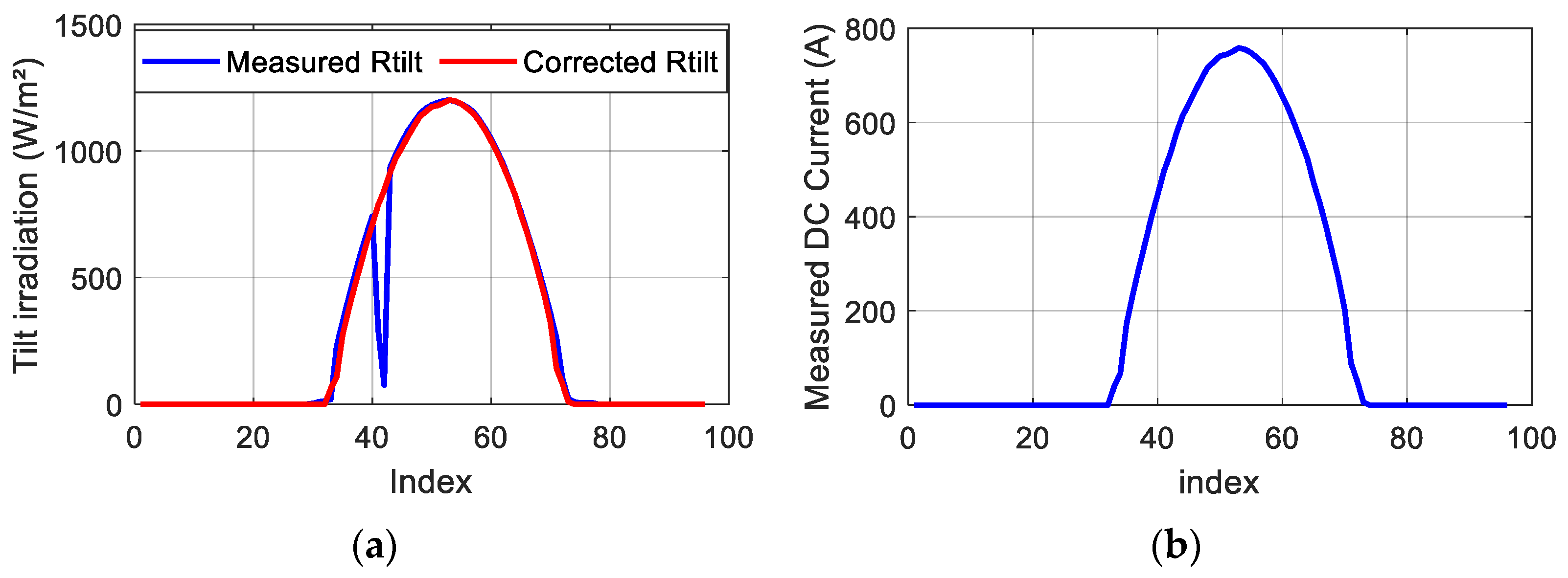
In our opinion, the main contributions of this work are as follows: (1) The integration of machine learning techniques with the analysis of power loss errors and current/voltage errors to detect and identify faults not only in PV modules but also in the irradiation sensor. While machine-learning models avoid the need for large databases by making predictions using reduced data samples, the analysis of power loss, voltage, and current errors provides robust and effective fault detection and identification. (2) The proposal of a novel method for correcting erroneous datasets, addressing environmental sensor inaccuracies that often hinder reliable performance prediction in PV systems. (3) A performance comparative study is also carried out with other machine learning techniques to justify the choice of RF and KNN predictive models. (4) The development and validation of various data-driven models for a large-scale, real-world grid-connected PV installation with a capacity of 500 kWp. The reliability of the fault detection and identification method is also validated using experimental data from the station.

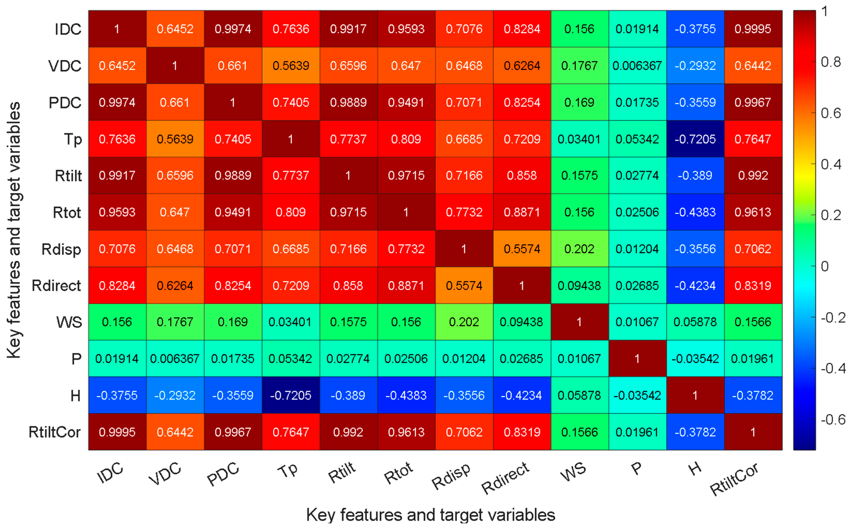
This paper is organized as follows: Section 2 presents an overview of the studied site and describes the PV power plant. Section 3 outlines the predictive models, including the data pre-processing process, tilt irradiation correction, and feature selection. Section 4 details the fault detection and diagnosis method based on the analysis of errors in power losses, DC voltage, and DC current. Finally, Section 5 and Section 6 discuss the results and present the main conclusions of this study.

2. Experimental Setup Description

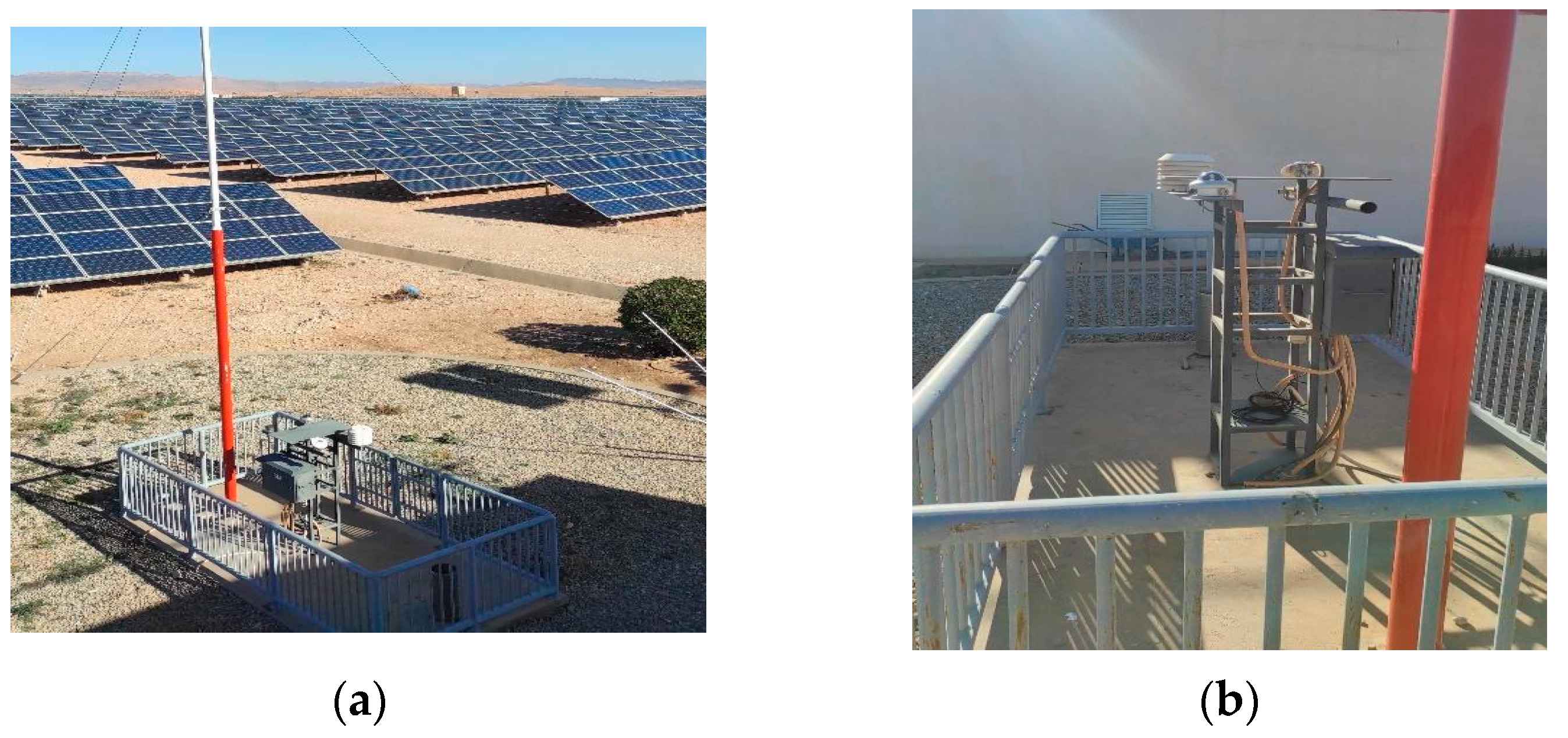
The dataset used in this study is collected from a grid-connected, ground-mounted photovoltaic (PV) system in Ain El-Melh, situated in the Algerian highlands near the desert region. Positioned at 34°51″ N latitude and 04°11″ E longitude, with an elevation of 910 m above sea level, the PV plant is integrated into the medium-voltage network of Ain El-Melh.

Part of a broader 400 MWp renewable energy initiative managed by SKTM, a subsidiary of Sonelgaz, this PV system contributes to Algeria’s commitment to advancing renewable energy. Under the Algerian government’s renewable energy directive, Sonelgaz has developed 23 PV power plants in the highlands and central regions. Spanning 40 hectares, the Ain El-Melh facility boasts an installed capacity of 20 MWp, designed to optimize energy production. The system utilizes polycrystalline silicon modules with a 15% efficiency rate, installed on fixed structures at a 33° tilt facing south to maximize solar exposure. To minimize shading and enhance energy capture, the rows of modules are spaced 5 m apart.

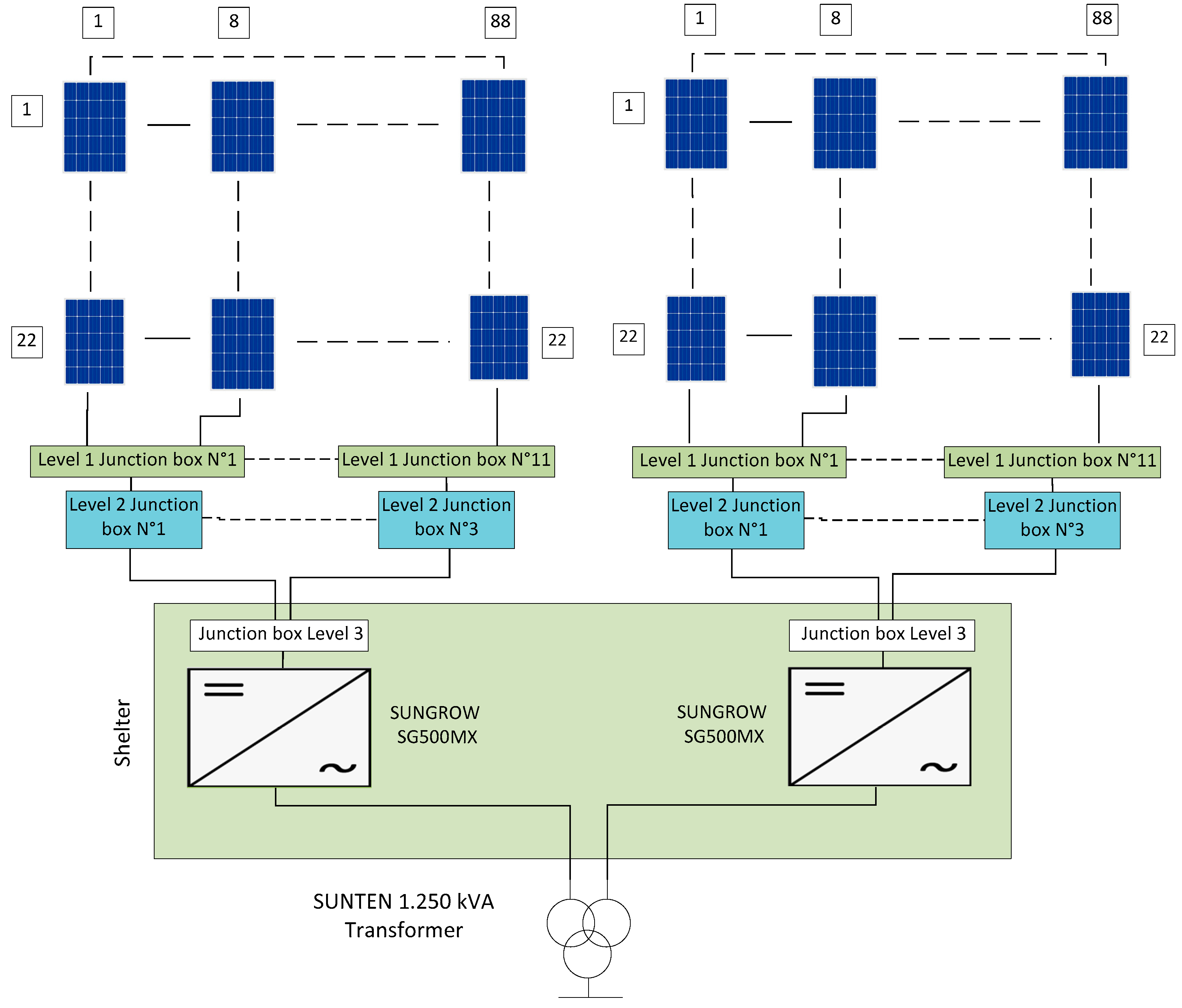
The solar park consists of 80,080 polycrystalline PV modules (250 Wp each) organized into 40 identical 500 kW sub-fields. Each sub-field consists of 1936 modules distributed over 88 strings (22 modules connected in series for each string). The PV modules are positioned at a 33° tilt and connected to a 500 kW SUNGROW inverter (500–850 VDC input, 315 VAC output). This configuration is consistently replicated across all sub-fields, where two sub-fields (totaling 1 MWp) share a 1250 kVA step-up transformer, as depicted in Figure 1. The electrical connection between the photovoltaic modules and their respective 500 kW inverter cabinets is performed via 11 junction boxes (level 1), 3 parallel boxes (level 2), and 1 general box (level 3), all housed in shelters. The use of a three-tiered grouping of boxes reduces the total length of DC cables and minimizes ohmic losses. Additionally, this design facilitates optimization and management (O&M) operations. The generated AC power is then transmitted via 60 kV overhead power lines to the national grid, maintaining a standardized layout for the 1 MWp blocks. This repeatable design ensures efficient energy flow from the modules through inverters and transformers. In this study, we will focus on the analysis, modeling, and fault diagnosis of the PV modules and DC power generation of only one 500 kW subfield.

The electrical and environmental dataset was collected from the inverters’ cabinet junction boxes. It includes a comprehensive range of parameters such as solar panel temperature, tilt irradiation, total irradiation, diffuse irradiation, direct irradiation, wind speed, humidity, pressure, voltage, current, and PV power, current, and voltage. The dataset was gathered throughout one year, from 1 January 2023 to 31 December 2023, with measurements taken at 15-min intervals. This resulted in a dataset containing 69,195 data points. A summary of the environmental and electrical parameters of the PV system for the year 2023 is listed in

Table 1. Summary of environmental and electrical parameters of the PV system.

Features	Description	Minimum	Maximum	Average
Tp	Panel temperature (°C)	−2.5000	74.8000	27.8800
Rtilt	Tilt irradiation (W/m2)	0	1565.7	308.2515
Rtot	Total irradiation (W/m2)	0	1395.6	237.9987
Rdisp	Dispersion irradiation (W/m2)	0	648	73.6811
Rdirect	Direct irradiation (W/m2)	0	1364.3	234.4052
WS	Wind speed (m/s)	0	22.2	3.7939
H	Humidity (%)	0	71.6000	35.2273
P	Pressure (Pa)	0	927	911.3952
VDC	Voltage (V)	0	780.4000	323.4112
IDC	Current (A)	0	944.3000	182.6364
PDC	Power (kW)	0	569.4410	107.6481

.

3. RF and KNN-Based Prediction Models

3.1. Data Processing

The data processing phase involved several critical steps in providing high-quality data for predictive modeling. Initially, raw data from the inverter cabinets and junction boxes were pre-processed to address inconsistencies, missing values, and outliers. Data points with significant errors or gaps were either interpolated or excluded to maintain reliability and completeness.

A key challenge was the correction of tilt radiation data, as the tilt radiation sensor was incorrectly positioned during site measurements, causing shading effects that did not occur on the PV modules themselves. To resolve this, tilt radiation values were adjusted by scaling them according to current variations, which were recorded simultaneously. This adjustment ensured that the tilt radiation data more accurately reflected the actual solar exposure received by the modules.

After data normalization, we removed biases introduced by differing measurement units or magnitudes. Feature selection techniques, such as correlation analysis and importance ranking, were employed to identify the most relevant parameters—such as solar panel temperature, radiation, and environmental conditions—while removing redundant or irrelevant features.

Following pre-processing, the dataset was split into training (80%) and testing (20%) subsets to evaluate the models’ generalization capabilities. These steps, mainly the tilt radiation correction, were crucial for addressing discrepancies identified during sensor validation. Figure 2 illustrates the environmental measurement station’s positioning within the solar park, highlighting how shading effects were resolved by scaling the tilt radiation against synchronized current readings.

3.1.1. New Correction Method of the Tilt Irradiation Data

Tilted irradiation $R_{tilt}$ plays a fundamental role in assessing the performance of PV systems. To ensure data reliability, we first evaluated the accuracy and consistency of the tilted irradiation measurements by comparing them with the output DC current, supplied by the PV system throughout the day. Our analysis revealed erroneous data within one specific time interval, requiring correction to enhance data accuracy. This correction is critical for improving the accuracy of prediction models. In view of this, we introduce a new correction method for tilt irradiation data. The core principle of the proposal is to restore the original irradiation values while incorporating an adjustment factor that accounts for variations in the DC current.

First, the collected DC current undergoes a scaling process. Using the min–max scaling method, the normalized values of DC current denoted $I_{DC,scaled}$ is:

$$I_{DC,scaled}={\displaystyle \frac{I_{DC}-I_{DC,\min }}{I_{DC,\max }-I_{DC,\min }}}$$

(1)

$I_{DC,\min }$ and $I_{DC,\max }$ are the minimum and maximum values of $I_{DC}$.

Thereafter, the correction of the tilted irradiation is carried out by leveraging the scaled current data to adjust the values of $R_{tilt}$. The proposed reconstruction equation is given as follows:

$$R_{tiltCor}=I_{DC,scaled}\times \left(R_{tilt,\max }-R_{tilt,\min }\right)+R_{tilt,\min }$$

(2)

$R_{tiltCor}$ is the corrected tilted irradiation derived from $I_{DC,scaled}$.$R_{tilt,\min }$ and $R_{tilt,\max }$ are the minimum and maximum values in the irradiation vector. The multiplication by $\left(R_{tilt,\max }-R_{tilt,\min }\right)$ rescales the tilted irradiation to match its original range, while the addition of $R_{tilt,\min }$ ensures proper re-adjustment within the expected values.

Figure 3a illustrates the waveforms of the uncorrected and corrected tilt irradiations, emphasizing the effectiveness of the proposed correction method in minimizing sensor-induced errors. An abrupt drop in the irradiation value is observed in the early morning, which is attributed to partial shading on the sensor caused by its positioning within the solar PV park. The corrected irradiation better aligns with the real behavior of the measured DC current depicted in Figure 3b, confirming the accuracy and reliability of the proposed correction method.

The term ‘index’ refers to the equidistant sample times at which data are collected to construct the numerical time series of the current and tilt irradiation. Given a constant sample acquisition time, this term simply represents the sample’s position in the dataset.

3.1.2. Features Selection

After cleaning and normalization of the training data, a Pearson correlation coefficient matrix was computed to assess the interdependencies between the features themselves on the one hand and between features and target variables (PV current, voltage, and power) on the other hand. In this paper, we use three target variables, including the supplied PV current, voltage, and power ($I_{DC}$, $V_{DC}$ and $P_{DC}$). The heatmap revealed several significant correlations guiding our feature selection process. Specifically, for predicting the PV power and current, the analysis identified strong correlations with key features, including module temperature, tilt irradiation, and global irradiation. These features were indeed found to have a crucial impact on the supplied power and current. As for the output PV voltage, the heatmap in Figure 4 revealed an almost perfect correlation between the tilt irradiation and the module temperature. Therefore, we eliminate the remaining inappropriate and redundant features and only focus on the most strongly correlated variables to minimize the risk of multicollinearity and ensure a more robust training process [33].

3.2. RF and KNN: Hyperparameters Tuning and Performance Evaluation

This study utilizes two machine learning models, Random Forest (RF) and K-Nearest Neighbors (KNN), optimized using the Grid Search technique, to predict photovoltaic module performance metrics, including power, current, and voltage.

3.2.1. Random Forest (RF)

The Random Forest (RF) algorithm is a robust and effective machine learning method utilized in this work to predict the supplied PV current and power. RF’s ability to capture complex nonlinear relationships between input and output variables and assess feature importance makes it particularly well-suited for regression tasks. Additionally, it provides a detailed analysis of the most influential factors, thereby offering better insights into the variables affecting photovoltaic system performance [34].

The RF algorithm is built upon multiple decision trees, which are hierarchical structures that recursively split the data based on feature values. In order to predict for a query point x, each tree makes its independent prediction. Thereafter, the forest makes the average of all decisions, as shown in Equation (3), which enhances accuracy and reduces the risk of overfitting.

$${\widehat{y}}^k(x)={\displaystyle \frac{1}{N}}{\displaystyle \sum _{j=1}^N{y}_j^k}(x)$$

(3)

${\widehat{y}}^k(x)$is the average of predictions from all the trees and N is the total number of trees. $y_j^k(x)$ is $j\mathrm{th}$ tree being trained from data of fold k.

The parameters of the RF model were optimized using the Grid Search method, a systematic approach that explores various combinations of hyperparameter values to maximize predictive accuracy. The initial hyperparameter ranges are selected based on established practices in the literature, empirical insights derived from the dataset, and the need to balance predictive performance with computational efficiency [35]. Considering this, the initial values of key hyperparameters are ranged as follows:

• Number of Trees (NumTrees): This parameter controls the number of decision trees in the forest. A higher number of trees generally improves the model’s stability and accuracy but increases computational cost and training time. The chosen initial values are [1, 50], [50, 100, 150].
• Minimum Leaf Size (MinLeafSize): This parameter determines the minimum number of observations required in a leaf node. Smaller values allow finer granularity but may lead to overfitting. The selected initial values are [50, 100, 200], [1, 5, 10].
• Maximum Number of Splits (MaxNumSplits): This limits the depth of individual trees, balancing the complexity and predictive performance of the model. The chosen initial values are [10, 20, 50].
• Split Criterion (Criterion): This defines the metric (e.g., mean squared error) used for splitting nodes during tree construction. The value selected was {‘mean squared error’}.

3.2.2. K-Nearest Neighbors (KNN)

The K-Nearest Neighbors (KNN) algorithm is a widely recognized, non-parametric technique for prediction, based on the principle of similarity. Its simplicity and computational efficiency make it ideal for small to medium-sized datasets, and its ability to model non-linear relationships allows it to effectively capture complex data patterns [36]. The core of KNN involves identifying the k closest neighbors to a given input (query point), which requires an effective way to measure the distances between data points. Several distance metrics are commonly used to determine proximity, depending on the problem and the nature of the data. Among the most prevalent are Euclidean Distance ($D_{euclidean}$), Cityblock Distance ($D_{Cityblock}$), and Chebyshev Distance ($D_{chebychev}$), defined by the following Equations (4a)–(4c):

$$D_{euclidean}(x_q,x_i)=\sqrt{{\displaystyle \sum _{j=1}^n{(x_{q,j}-x_{i,j})}^2}}$$

(4a)

$$D_{Cityblock}(x_q,x_i)={\displaystyle \sum _{j=1}^n\left|x_{q,j}-x_{i,j}\right|}$$

(4b)

$$D_{chebychev}(x_q,x_i)=\underset{j}{\max }\left|x_{q,j}-x_{i,j}\right|$$

(4c)

$x_{q,j}$ and $x_{i,j}$ represent the $j\mathrm{th}$ feature of the query point and the training point, respectively. The choice of distance metric impacts how the model captures the relationship between features. Once the appropriate value of k is selected, the prediction is computed using KNN by averaging the k nearest neighbors:

$$\widehat{y}={\displaystyle \frac{1}{k}}{\displaystyle \sum _{i=1}^k{y}_i}$$

(4d)

$\widehat{y}$ is the predicted output using the KNN and $y_i$ is the label (or output value) of the $i\mathrm{th}$ nearest neighbor.

In this paper, we make use of the KNN algorithm to forecast the output voltage supplied by the PV system. The model was optimized through the Grid Search method [37], which fine-tuned several critical hyperparameters for improved prediction accuracy. The key hyperparameters adjusted in the process include:

• Number of Neighbors (k): The selected values and ranges are (k = 10) [1, 10] and [3, 5, 7, 9].
• Distance Metric (Distance): The selected values are {‘euclidean’, ‘cityblock’, ‘chebychev’}.
• Standardization (Standardize): This parameter controls whether the features should be normalized to a common scale. Standardization ensures that each feature contributes equally to the model, preventing any individual variable from exerting undue influence due to differing scales or units. The chosen values were {‘true’, ‘false’}.

3.2.3. Cross-Validation and Evaluation Metrics

To ensure the robustness and generalization capabilities of the models, 10-fold cross-validation was incorporated into the hyperparameters tuning process. The dataset was divided into 10 subsets, with nine folds used for training and the remaining fold for validation. This process was repeated 10 times, allowing each fold to serve as the validation set once. The final performance metric was obtained by averaging the results across all folds [14,38].

In addition to cross-validation, several performance metrics were utilized to evaluate the predictive models developed for the PV system. These metrics, including the R² (Coefficient of Determination), RMSE (Root Mean Squared Error), and MAE (Mean Absolute Error), provided a comprehensive assessment of the models’ accuracy and reliability. The R² metric quantifies the proportion of variance in the target variable explained by the model, with values closer to 1 indicating a better fit. This was calculated using Equation (5a):

$${\mathrm{R}}^2=1-{\displaystyle \frac{{\displaystyle \sum _{i=1}^n{\left(y_i-{\stackrel{\wedge }{y}}_i\right)}^2}}{{\displaystyle \sum _{i=1}^n{\left(y_i-\overline{y}\right)}^2}}}$$

(5a)

where $y_i$ represents the observed values, ${\stackrel{\wedge }{y}}_i$ represents the predicted values, $n$ is the sample size, and $\overline{y}$ is the mean of the observed values.

The RMSE quantifies the average magnitude of the errors between the predicted and actual values, with lower values indicating better model performance. It is calculated as:

$$\mathrm{RMSE}=\sqrt{{\displaystyle \frac{1}{n}}{\displaystyle \sum _{i=1}^n{\left(\left(y_i-{\stackrel{\wedge }{y}}_i\right)\right)}^2}}$$

(5b)

Finally, the MAE measures the average of the absolute errors between the predicted and observed values, providing an interpretable measure of prediction accuracy. It is given by Equation (5c):

$$\mathrm{MAE}={\displaystyle \frac{1}{n}}{\displaystyle \sum _{i=1}^n\left|y_i-{\stackrel{\wedge }{y}}_i\right|}$$

(5c)

4. Proposed Fault Detection and Diagnosis Method

Power losses in PV systems are crucial factors that directly impact their overall performance and efficiency. These losses arise from environmental and operational conditions, such as shading, dirt accumulation, and module temperature variations. Deviations from standard test conditions often lead to reduced efficiency in real-world settings. For example, when module temperatures rise above the standard 25 °C, energy losses occur, and additional inefficiencies may arise due to factors like maximum power point tracking failures, module mismatches, and partial shading. These power losses act as key indicators that can help detect faults early in the system, making it possible to diagnose and address issues before they lead to more significant inefficiencies or damage.

Therefore, fault detection and isolation through automated supervision systems have become crucial for notifying the operator to take corrective actions, such as reconfiguring the PV array layout or replacing defective modules. These actions, in turn, will reduce maintenance costs, maximize power production, and prevent long-term degradation of the PV array.

Various faults, such as string disconnection, short-circuited modules, and shading, contribute to significant power losses. For example, a string disconnection results in the complete loss of power from the affected string, while short-circuited modules cause excessive current flow, leading to overheating and further energy losses. Additionally, shading can reduce overall energy generation, especially in systems with series-connected panels. Monitoring these power losses and their deviations from expected output is essential, allowing for early detection of faults and targeted corrective actions. Timely and accurately classifying these faults ensures minimal energy loss and helps maintain the system’s reliability, ensuring it performs optimally.

Table 2. Types of faults in PV systems and their importance.

Fault Type	Location	Reasons	Importance of Detection and Diagnosis
String Disconnection	Photovoltaic String	Disconnection of one or more panels in a string due to wiring or connector failure.	Vital for identifying power loss from part of the system and ensuring maximum energy output. Timely detection facilitates quick repairs and reduces system downtime.
Short-Circuited Module	Module	Faults within a single module caused by defective components or wiring issues, resulting in abnormal current flow.	Crucial for preventing overheating, damage to the module, and potential cascading effects on the system. Early detection helps avoid further damage and ensures system safety.
Shading	Panel Array	Partial or complete obstruction of sunlight due to nearby objects (trees, buildings, dirt, etc.).	Important for detecting performance degradation in shaded areas. Identifying shading allows for corrective measures such as repositioning or cleaning panels, and optimizing energy output.

outlines the various types of faults commonly encountered in photovoltaic systems, along with their locations, underlying causes, and the importance of timely detection and diagnosis for maintaining system efficiency and reliability [39,40].

By focusing on the power loss factors, the following sub-sections highlight how they can be utilized to identify inefficiencies and malfunctions within the system. This approach paves the way for proactive diagnostic strategies, which not only aid in the early detection of faults but also play a crucial role in improving the system’s overall performance.

4.1. Identification of Performance Indicators in a PV System

In this part, we delve into key performance indicators, which are essential for assessing the efficiency and health of photovoltaic systems [41]. The Reference Yield ($Y_r$) [h/d] represents the amount of time, expressed in hours per day, required to accumulate an equivalent amount of instantaneous solar irradiation as that received under the reference irradiation level and is calculated using Equation (6).

$$Y_r={\displaystyle \frac{H_I}{G_{STC}}}$$

(6)

$H_I$ refers to the solar irradiation on the module plane, expressed in kWh/m² per day, while $G_{STC}$ represents the irradiation under standard test conditions (STC), set at 1000 W/m².

The Array Yield ($Y_a$) [h/d] represents the total hours per day the PV array operates at its maximum power to generate energy. It is computed as follows:

$$Y_a={\displaystyle \frac{E_{DC}}{P_{rated}}}$$

(7)

$E_{DC}$ represents the DC electricity generation of the photovoltaic array, measured in kWh per day, while $P_{rated}$ refers to the rated power of the PV plant, expressed in kilowatts peak (kW_p).

The Final Yield ($Y_f$) [h/d] represents the number of hours per day during which the PV system operates at its rated power. It is determined as follows:

$$Y_f={\displaystyle \frac{E_{Ac}}{P_{rated}}}$$

(8)

$E_{Ac}$ represents the AC electricity generation, measured in kWh per day.

The Performance Ratio $PR$ [%] is a quality factor of the PV system rather than a direct efficiency measure. It reflects the extent to which the system’s performance is impacted by accumulated losses, showing how the actual system deviates from an ideal PV system with no losses. This ratio also enables comparisons between different plants operating under various climatic and environmental conditions. It is defined as the ratio of the final yield to the reference yield:

$$PR={\displaystyle \frac{Y_f}{Y_r}}$$

(9)

4.2. Identification of Power Loss Factors

Capture losses primarily occur on the DC current side of the PV conversion process, influenced by various factors such as operating temperature, temperature sensitivity, PV efficiency, fluctuations in solar irradiation, shading effects, and losses due to high angles of incidence (AOI) of sunlight. Other additional losses within the PV array arise from issues like inaccuracies in maximum power point tracking (MPPT), module parameter mismatches, wiring losses, and the effects of aging on the system. In a predictive model of a PV plant, the effective irradiation and module temperature serve as key inputs, enabling the calculation of predicted capture losses ($L_{c\_pred}$)—excluding operational faults—as follows:

$$L_{c\_pred}=Y_r(G,T_c)-Y_{a\_pred}(G,T_c)$$

(10)

$Y_r(G,T_c)$ and $Y_{a\_pred}(G,T_c)$ are the measured reference yield and predicted yield under an irradiation G and PV module’s temperature T_c.

On the other hand, thermal capture losses represent a factor providing valuable insights into energy losses caused by thermal effects under real-world operating conditions. The predicted normalized thermal capture losses $L_{ct\_pred}$ are defined as the difference between the yield predicted at standard temperature and that predicted at the real PV module’s operating temperature [42]:

$$L_{ct\_pred}=Y_{a\_pred}(G,25 \text{°}\mathrm{C})-Y_{a\_pred}(G,T_c)$$

(11)

$Y_{a\_pred}(G,25 °\mathrm{C})$ is the normalized energy yield at real-working irradiation and a standard temperature of 25 °C, while $Y_{a\_pred}(G,T_c)$ denotes the array yield at real-working irradiation and module’s temperature T_c.

Miscellaneous capture losses encompass a range of inherent losses, including wiring inefficiencies, string diode losses, low irradiation, dirt accumulation, non-uniform irradiation, module mismatches, maximum power point tracking (MPPT) errors, and DC-side failures such as faulty strings, defective modules, partial shading, and short circuits. The predicted miscellaneous capture losses $L_{cm\_pred}$ are determined in terms of capture losses and thermal capture losses as follows:

$$L_{cm\_pred}=L_{c\_pred}-L_{ct\_pred}$$

(12)

4.3. Fault Detection Based on the Analysis of the Miscellaneous Capture Loss Error

Define the error $E{L}_{cm}$, which quantifies the deviation between the measured miscellaneous capture losses ($L_{cm\_meas}$) and their predicted counterpart ($L_{cm\_pred}$), such that:

$$E{L}_{cm}=L_{cm\_meas}-L_{cm\_pred}$$

(13)

Therefore, the fault detection in the PV system is performed through continuous monitoring of $E{L}_{cm}$, serving also as a key metric for assessing the accuracy of the prediction models. To reduce the risk of false fault detections, it is crucial to establish a well-defined threshold for $E{L}_{cm}$, which delineates the permissible deviation range between predicted and measured values. Considering this, the upper and lower limits of $E{L}_{cm}$, representing the healthy state of the PV system are given as:

$$E{L}_{cm\_ref}-k{\delta }_{Lcm}<E{L}_{cm}<E{L}_{cm\_ref}+k{\delta }_{Lcm}$$

(14)

$E{L}_{cm\_ref}$ is the reference deviation in healthy conditions between the measured and predicted miscellaneous capture losses, referred to as $L_{cm\_meas(fault\_free\_conditions)}$ and $L_{cm\_pred(fault\_free\_conditions)}$, respectively:

$$E{L}_{cm\_ref}=L_{cm\_meas(fault\_free\_conditions)}-L_{cm\_pred(fault\_free\_conditions)}$$

(15)

${\delta }_{Lcm}$ is the standard deviation of $E{L}_{cm}$, calculated using the dataset of one day in healthy conditions. It is obtained as 0.0031. k is a constant, empirically adjusted to 1.25.

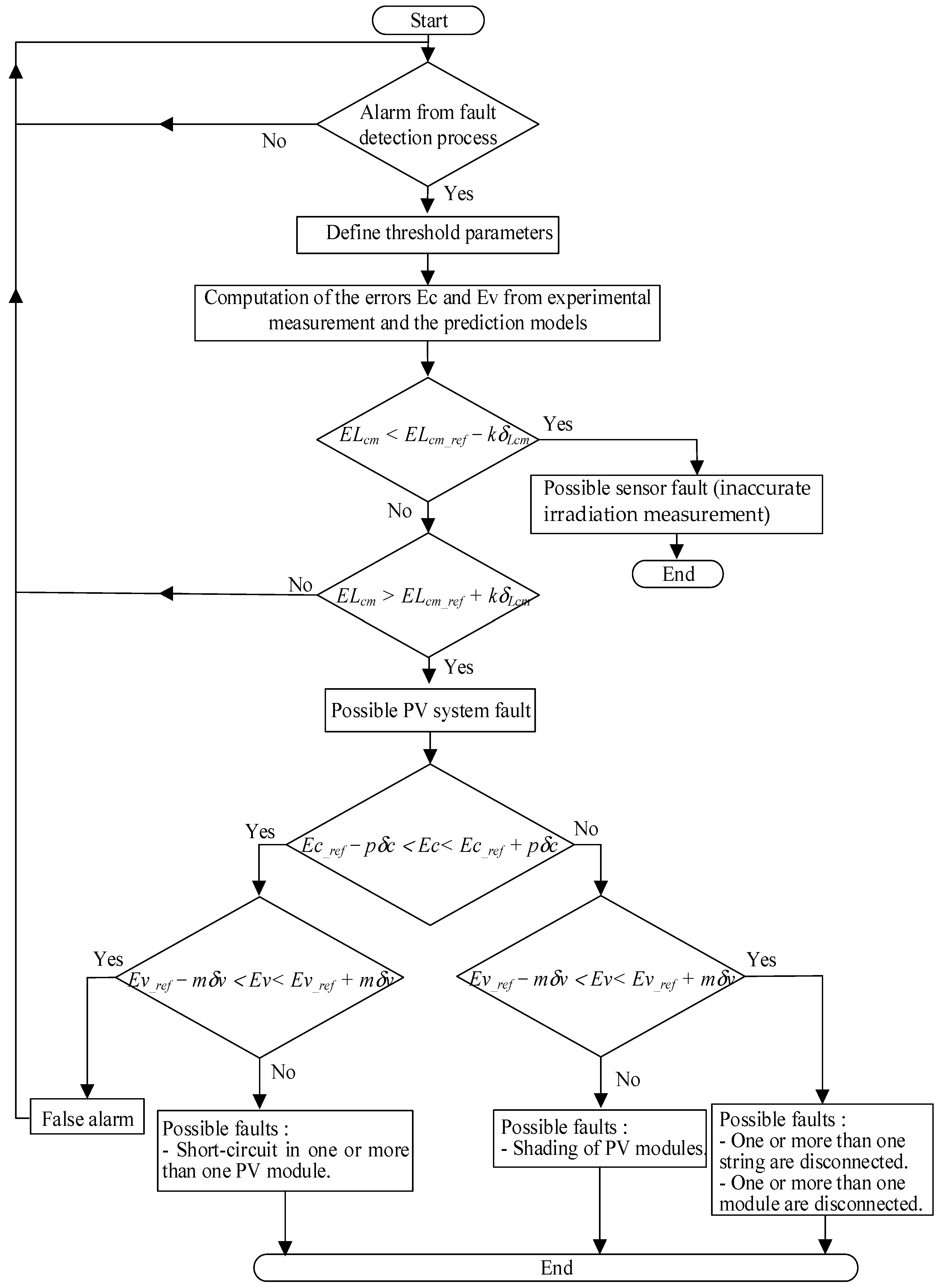
Figure 5 presents the flowchart of the fault detection procedure, illustrating the decision-making process for fault identification based on the analysis of the miscellaneous loss error between the actual power measurements and the predicted power by the RF model.

4.4. Fault Diagnosis

When the error indicator $E{L}_{cm}$ exceeds the predefined threshold band, indicating a potential fault. The next step is to diagnose the root cause of the anomaly. To isolate the fault and identify its type, we use, in addition to $E{L}_{cm}$, two electric indicators: the DC current error ($E_c$) and the DC voltage error ($E_v$). These indicators quantify the deviations between the measured and predicted DC current and voltage values, respectively, and are calculated as follows [23]:

$$E_c=I_{DC\_meas}-I_{DC\_pred}$$

(16)

$$E_v=V_{DC\_meas}-V_{DC\_pred}$$

(17)

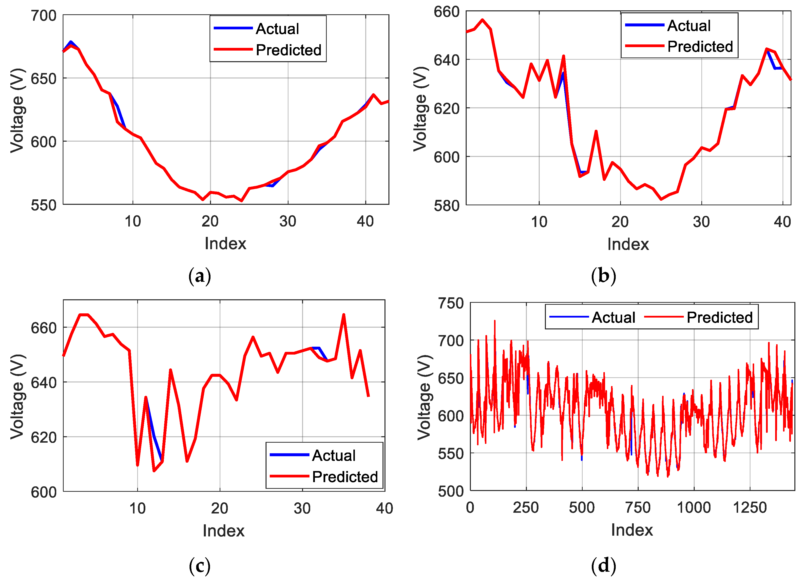
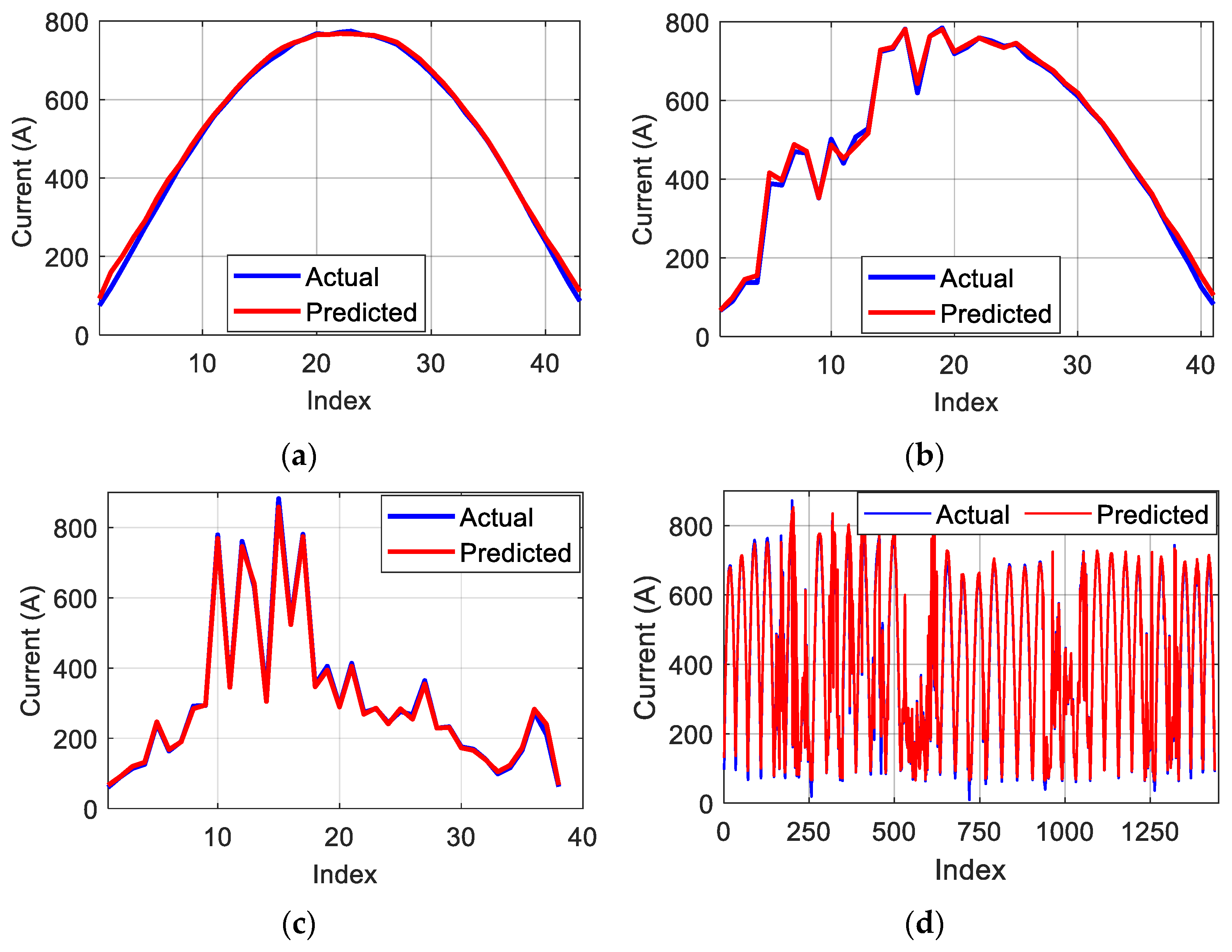
$I_{DC\_meas}$ and $V_{DC\_meas}$ are the measured DC current and voltage, respectively. $I_{DC\_pred}$ is the predicted current using the RF model, while and $V_{DC\_pred}$ is the predicted voltage using the KNN model.

Similarly, in order to avoid a false fault isolation, we define the upper and lower limits beyond which the error is confirmed:

$$E{c}_{ref}-p{\delta }_c<Ec<E{c}_{ref}+p{\delta }_c$$

(18)

$$E{v}_{ref}-m{\delta }_v<Ev<E{v}_{ref}+m{\delta }_v$$

(19)

$E{c}_{ref}$ is the reference deviation in healthy conditions between the measured and predicted DC current supplied by the PV plant namely $I_{DC\_meas(free\_fault\_conditions)}$ and $I_{DC\_pred(free\_fault\_conditions)}$, respectively:

$$E{c}_{ref}=I_{DC\_meas(free\_fault\_conditions)}-I_{DC\_pred(free\_fault\_conditions)}$$

(20)

$E{v}_{ref}$ is the reference deviation in healthy conditions between the measured and predicted DC Voltage provided by the PV plant, referred to as $V_{DC\_meas(free\_fault\_conditions)}$ and $V_{DC\_pred(free\_fault\_conditions)}$, respectively:

$$E{v}_{ref}=V_{DC\_meas(free\_fault\_conditions)}-V_{DC\_pred(free\_fault\_conditions)}$$

(21)

${\delta }_c$ = 10.4535 and $\delta v$ = 2.0964 are the standard deviations of $Ec$ and $Ev$, respectively, obtained from a collected dataset of one day in healthy conditions. p and m are two constants, empirically adjusted to 0.5 and 0.4.

Considering this, the diagnosis method aims first at identifying if the fault is actually affecting the PV system or if it is only due to sensor malfunction. This partition is performed through the analysis of the miscellaneous capture loss error deviation outside the threshold band as follows:

• Sensor faults—Detected when $E{L}_{cm}$ falls below the lower threshold limit. This fault is likely due to a shading issue affecting only the pyranometer, without being propagated to the PV modules and leading to an inaccurate irradiation measurement.
• PV System Faults—Identified when $E{L}_{cm}$ surpasses the upper threshold limit, indicating potential operational inefficiencies or system degradation.

This approach ensures a precise differentiation between system-level faults and sensor malfunctions, leading to more accurate fault diagnosis. Furthermore, it can be generalized to any grid-connected PV system, allowing for system-specific threshold calibration to enhance fault detection reliability.

In the second stage, once the fault source comes effectively from the PV system itself, additional processing is performed to isolate four possible fault sources. The proposed identification method relies on the analysis of the two electric indicators $E_c$ and $E_v$, considering their location within or outside their respective threshold bands. The following four scenarios are, therefore, useful for identifying the possible sources of faults in the PV system:

• $E_c$ and $E_v$ are both located outside their respective threshold bands: the PV system might be affected by shading.
• $E_c$ remains within the threshold band while $E_v$ is outside: this might be caused by a short-circuit of PV modules.
• $E_c$ is located outside the threshold band while $E_v$ remains inside: this situation might be caused by a disconnection problem affecting the PV modules, or strings.
• $E_c$ and $E_v$ are both located inside their respective threshold bands: it is a false alarm announced by the fault detection algorithm, and the PV system is still operating in a healthy condition.

The flowchart of Figure 6 summarizes the fault diagnosis procedure, illustrating different tests performed to isolate the possible cause of the fault or even detect a false alarm.

5. Results and Discussion

5.1. Assessment of the Predictive Models Performance and Comparison with Other Models

We first evaluated the effectiveness of the models in predicting the voltage current and power provided by the PV system under different weather conditions including clear skies, semi-cloudy, and cloudy days. The predicted outputs for voltage, current, and power are compared with the measured values. The evaluation is made considering a dataset collected during one operating day. Additionally, we used a dataset that spanned 36 days, three from each month of the year to assess the prediction model’s ability to capture the long-term variability introduced by different seasons and environmental conditions. Note that all datasets were collected from measurements performed at the DC side of the PV system, operating at its maximum power point.

5.1.1. DC Voltage Prediction Using the K-Nearest Neighbors

Figure 7a illustrates the predicted DC voltage using the KNN model and the measured values under a clear sky condition. As can be seen, the predicted voltage closely follows the measurement. This is corroborated by the regression metrics listed in

Table 3. Regression metrics of the DC voltage prediction-based KNN model.

Model	Condition	R2	RMSE (V)	MAE (V)
KNN (Voltage Prediction)	Clear skies	0.99674	2.0662	0.54651
	Semi-cloudy	0.99523	1.5509	0.41951
	Cloudy	0.97851	2.1214	0.42368
	36-day period	0.98263	5.101	0.95511

, where the coefficient of determination (R²) is about 0.99674, indicating an almost perfect fit. This test scenario provides the lowest RMSE and MAE obtained, as 2.0662 V and 0.54651 V, respectively, confirming minimal deviation between predictions and real values. The adaptability and robustness of the model in stable weather conditions is therefore proved.

The results depicted in Figure 7b were obtained from a test scenario with semi-cloudy conditions. The prediction model still performs well, with an R² of 0.99523, demonstrating strong predictive ability. The slight increase in RMSE (1.5509 V) and MAE (0.41951 V) remains acceptable, considering the operating voltage varies from approximately 580 V to 650 V. In the test scenario of a cloudy day, the results shown in Figure 7c indicate that the model’s performance slightly declines, though it remains relatively robust. The R² value drops to 0.97851, indicating a slight decrease in predictive accuracy. Additionally, the RMSE and MAE increased to 2.1214 V and 0.42368 V, respectively. This increase in errors is also acceptable, as the real operating voltage across the PV system remains within the range of [610 V, 670 V].

Figure 7d depicts the predicted and measured output voltage across a 36-day period throughout the year. The results show a modest decline in predictive performance, with the R² dropping to 0.98263 and the RMSE increasing to 5.101 V. The MAE also rises significantly to 0.95511 V.

In our opinion, the increase in the statistical metrics RMSE and MAE compared to the one-day test results is mainly due to the following key factors:

-

Significant seasonal variations in environmental conditions in the region of “Ain El Melh” introduce a higher degree of heterogeneity in the 36-day test dataset compared to the one-day test. For example, fluctuations in solar irradiance, temperature, and weather patterns add variability and noise, which reduce the model’s ability to generalize effectively. In contrast, short-term predictions benefit from a more homogeneous dataset, which is typically easier for the model to handle.

-

Error accumulation over time can amplify discrepancies. Small inaccuracies in early predictions may compound over multiple days, resulting in a noticeable increase in RMSE and MAE for long-term forecasts.

It is worth mentioning that the performance decrease observed in long-term predictions has no substantial impact on the outcomes related to fault detection and identification. This process is primarily conducted over short time periods and relies mainly on accurate short-term predictions. Overall, the results confirm that the KNN model is highly effective for voltage prediction in a PV system, particularly under stable weather conditions. However, long-term variations in weather and seasonal effects lead to a slight decrease in performance.

5.1.2. DC Current Prediction Using Random Forest

The four aforementioned test scenarios were also carried out to evaluate the performance of the RF model in predicting the DC current provided by the PV system. The obtained results are shown in Figure 8a–d. The RF model closely follows the measured values, with R² values exceeding 0.9965 in the three daily scenarios, as listed in

Table 4. Regression metrics of DC current prediction using RF models.

Model	Condition	R2	RMSE (A)	MAE (A)
Random Forest (Current)	Clear skies	0.99657	13.1248	9.3406
	Semi-cloudy	0.99702	12.2937	9.2768
	Cloudy	0.99791	9.5031	9.5031
	36-day period	0.99604	13.908	9.911

. The MAE ranges from 9.34 A to 9.9 A, while the RMSE remains within the range [9.5 A, 13.9 A]. Once again, the obtained performance metrics remain acceptable, considering that the output current may approach 800 A during peak production. However, the accuracy has degraded compared to the voltage prediction model. In our opinion, this is due to the complex behavior of the current supplied by the PV systems, which varies non-linearly with several weather and electrical parameters.

On the other hand, the long-term predicted results obtained over a 36-day period show practically similar performance compared to daily predictions in terms of R² obtained as 0.99604, with a slight increase of RMSE and MAE to 13.908 A and 9.911 A, respectively.

5.1.3. Power Prediction Using Random Forest

The predicted and measured output power for the four test scenarios are illustrated in Figure 9a–d. These results show that the RF model provides high accuracy in predicting the daily PV output power, with R² values consistently above 0.99 across different weather conditions, as listed in

Table 5. Regression metrics of PV power prediction using RF models.

Model	Condition	R2	RMSE (kW)	MAE (kW)
Random Forest (Power)	Clear skies	0.99459	8.7315	6.1849
	Semi-cloudy	0.99664	7.5305	5.6593
	Cloudy	0.9959	8.1518	5.2588
	36-day period	0.99471	9.0827	6.3852

. The MAE decreased from 6.18 kW under clear skies conditions to 2.25 kW under cloudy skies. Similarly, the RMSE decreased from 8.73 kW under clear skies to 8.15 kW under semi-cloudy skies. The reduction in MAE and RMSE in the cloudy and semi-cloudy scenarios is due to the narrower output power production range, as less solar energy is received by the PV cells. Overall, the obtained daily performance metrics remain acceptable, considering that the maximum supplied PV power exceeds 400 kW during peak production. Nevertheless, the accuracy has degraded compared to the voltage prediction model.

The prediction performance of the output power over a 36-day period shows nearly identical results in terms of R² and MAE, with values of 0.99471 and 6.3852 kW, respectively. A slight increase in RMSE is observed, rising to 9.0827 kW. Overall, the obtained outcomes suggest that the model performs accurately and is well adapted to long-term seasonal variations.

5.1.4. Evaluation of Models with Statistical ANOVA and Comparison with Other Methods

To further evaluate the performance of the proposed predictive models, we conducted a one-way Analysis of Variance (ANOVA) test on the predicted and measured datasets. The goal was to assess whether significant differences existed between the two groups of measured and predicted data. Figure 10a–c present the notched boxplots of the predicted and measured values for voltage, current, and power, with corresponding statistical data listed in

Table 6. Statistical performance obtained from one-way ANOVA test.

	Median	Lower Quartile	Upper Quartile	p-Value
Predicted voltage with KNN	592.7 V	564 V	625.9 V	0.97549
Measured Voltage	592.7 V	563.8 V	628.3 V
Predicted current with RF	571.7 A	344.1 A	730.7 A	0.85844
Measured current	565.7 A	329.5 A	720.7 A
Predicted power with RF	331.1 kW	214.7 kW	409 kW	0.83652
Measured power	327.7 kW	209.3 kW	405.9 kW

. The graphs show a close overlap between the notches of each data group. Moreover, the medians and quartiles (upper and lower) are highly consistent between actual and predicted values, particularly for voltage predicted by KNN, where the difference between the two medians is exactly zero. For current and power predictions using RF, the median errors increase slightly, reaching 6 A for DC current and 3.4 kW for generated power. However, this gap is not statistically significant, considering that the data distribution may exceed 800 A and 400 kW at peak production.

The probability of variance of data (p-value) analysis further supports this finding, as it indicates the statistical significance of any observed differences. The p-value is the probability of obtaining the observed results, or more extreme ones if the null hypothesis (H0) is true. The results in Table 6 show that the KNN model for voltage prediction achieves a p-value of 0.97549, indicating a high level of confidence in the model’s performance. Additionally, the Random Forest (RF) method produces p-values of 0.85844 and 0.83652 for current and power predictions, respectively, suggesting that the RF model also performs well, though with slightly less statistical significance. The obtained high p-values suggest that differences between the two groups of measured and predicted data are not statistically different and the null hypothesis is effectively true.

These visual and p-value statistical analyses, along with the high R² values already reported, prove the effectiveness and accuracy of the prediction models.

To better justify the choice of KNN and RF-based prediction models, we conducted a comparison with other models, including backpropagation (BP), linear regression (LR), and gradient boosting (GB). Additionally, since the primary objective of this paper is fault diagnosis of PV systems, we focus only on daily prediction models, as this task is performed over short periods during the day.

Table 7. Performance comparative analysis between different machine learning techniques.

	R2	RMSE	MAE
DC Voltage prediction (RMSE and MAE are in V)
BP	0.94915	8.2408	6.9904
LR	0.95629	7.6408	6.7154
GB	0.98765	4.1225	3.2721
RF	0.98999	3.6569	2.3342
KNN	0.99674	2.0662	0.54651
DC current prediction (RMSE and MAE are in A)
BP	0.9952	15.5277	12.2638
LR	0.99419	17.0888	14.1119
GB	0.99524	15.4678	11.8683
RF	0.99657	13.1248	9.3406
KNN	0.99022	22.1634	14.914
Power prediction (RMSE and MAE are in kW)
BP	0.99331	9.7078	6.9993
LR	0.98003	16.7801	13.2276
GB	0.99271	10.1392	7.7283
RF	0.99459	8.7315	6.1849
KNN	0.9921	10.5518	8.9316

hereafter, summarizes the key prediction performance obtained with different machine learning techniques, including the R², RMSE, and MAE.

For voltage predictions, KNN is the best performer with the lowest RMSE (2.0662 V), highest R² (0.99674), and lowest MAE (0.54651 V). RF follows closely with RMSE of 3.6569 V and R² of 0.98999. Gradient Boosting GB and LR perform well but are less effective than KNN and RF. BP shows the lowest performance among the models. In contrast, for current prediction, RF leads with an RMSE of 13.1248 A, R² of 0.99657, and MAE of 9.3406 A. GB performs similarly but slightly lags behind RF. BP and LR provide comparable performance, though KNN shows the worst results with the highest RMSE and MAE. As for power prediction, RF is the top performer with an RMSE of 8.7315 kW, R² of 0.99459, and MAE of 6.1849 kW. GB and KNN follow with similar performance, while Linear Regression (LR) is the least effective, with the highest RMSE (16.7801 kW) and lowest R² (0.98003).

In light of the above, the selection of KNN for voltage prediction and RF for current and power prediction is well justified, as they consistently provide the best balance of accuracy across these predicted PV output parameters.

5.1.5. Applicability of the Models to Other Regions or Climates

The applicability of the model to other regions or climates is an important consideration. While the model has been validated for this particular location, we recognize that environmental factors, such as solar radiation intensity, temperature fluctuations, and local weather conditions, can vary significantly across regions, which might affect the model’s performance. For instance, PV systems in regions with cloudier or rainy conditions, or those with higher humidity, could experience different performance degradation patterns compared to systems in arid or desert climates like “Ain El Melh”.

To address this limitation, future work will explore the applicability of the proposed model in different geographical contexts. This could involve applying the model to data from PV plants in diverse climates, such as tropical, temperate, or high-altitude regions. Moreover, even though the method remains valid, we plan to investigate the model’s adaptability to varying environmental factors by adjusting the input parameters, such as irradiance and temperature, based on the specific climate characteristics of the region.

5.2. Faults Detection and Diagnosis Validation

The faults detection and diagnosis were experimentally validated using a 500 kW_p grid-connected PV system located in Ain El Melh, Algeria, which was previously detailed in Section 2. During the validation process, the following types of faults were successfully identified: a disconnected string, a short-circuited module, partial shading, and sensor malfunctions.

5.2.1. Healthy Day

To assess the reliability of the predictive model under optimal conditions, system performance was evaluated on a healthy day, meaning a day free of operational faults. Figure 11a shows that the predicted array yields closely match the actual measured values, demonstrating exceptional forecasting accuracy. This consistency highlights the system’s reliability in predicting power generation when operating without disruptions, a crucial factor in optimizing energy distribution and management.

Beyond power yield predictions, system efficiency remains steady throughout the day. Figure 11b illustrates that miscellaneous capture loss error is consistently maintained within predefined reference thresholds. This suggests that the system experiences minimal efficiency losses, ensuring solar energy is effectively captured and converted.

Electrical stability further reinforces the system’s robustness. As depicted in Figure 11c,d, both DC current and voltage error thresholds remain within their expected operational limits. The absence of significant fluctuations in these parameters confirms that the system is functioning optimally, without any underlying electrical anomalies. This level of precision is essential for maintaining uninterrupted power generation and preventing potential failures.

These results provide a valuable reference point for detecting future anomalies and improving fault diagnosis in photovoltaic installations.

5.2.2. One-String Disconnection Fault

The analysis of this fault type is initially based on the obtained array yields and the resulting miscellaneous capture loss error, as illustrated in Figure 12a and Figure 12b, respectively. Although the discrepancies between the predicted and measured array yields are not significant, the miscellaneous capture loss error parameter experiences noticeable deviations beyond the threshold band. The sharp increase in capture loss error implies that the fault actively affects energy conversion efficiency.

A closer look at the electrical parameters provides additional insights into the nature of the fault. As depicted in Figure 12c, the current error parameter exceeds its predefined limits, indicating an imbalance in power flow due to the disconnected string. However, the voltage error parameter, shown in Figure 12d, remains within permissible bounds, further distinguishing this issue from other potential system failures. This specific behavior, where the current deviates beyond normal thresholds while the voltage remains stable, enables precise fault classification as a disconnected string.

5.2.3. Short-Circuit of One PV Module

By inspecting Figure 13a, we observe that the measured array yields show a small decrease in all samples compared to the predicted values, indicating unexpected power loss within the system. This discrepancy is further reflected in Figure 13b, where the miscellaneous capture loss error parameter exceeds its predefined upper threshold, confirming the presence of an operational anomaly.

The electrical analysis provides further insights into fault classification. Figure 13c shows that the DC current error remains largely within its expected operational range, indicating that the total current generated by the string is not significantly affected, likely due to the bypass effect of the remaining healthy modules. However, Figure 13d highlights a substantial deviation in the DC voltage error, which falls below the predefined lower limit of the fault threshold due to a localized voltage drop within the string. This specific fault signature, where the voltage error deviation exceeds normal limits while the current error remains within acceptable bounds, enables precise fault classification as a module short-circuit.

5.2.4. Partial Shading

Shading leads to a progressive reduction in output power, often impacting multiple modules and causing non-linear performance degradation. The results depicted in Figure 14a, show that the measured array yields experience a noticeable drop compared to the predicted values, indicating a reduction in power generation due to the shading effect. This deviation is further reflected in Figure 14b, where the miscellaneous capture loss error parameter significantly exceeds the predefined upper limit of the reference thresholds, confirming the presence of an operational anomaly. This increase in capture losses suggests that the system is unable to fully convert the available solar irradiation into electrical power, a typical characteristic of shading-induced losses. Moreover, compared to electrical faults such as short-circuits or string disconnections, the change in both array yields and miscellaneous capture loss error is much more important, with important and abrupt changes in their amplitudes during the day.

The electrical behavior under partial shading conditions provides further diagnostic insights. In Figure 14c, the DC current error parameter far exceeds the predefined fault threshold, with abrupt changes in its amplitude throughout the day. Simultaneously, Figure 14d shows that the DC voltage error parameter also surpasses both the predefined upper and lower threshold limits, reinforcing the evidence of abnormal operating conditions. This unique fault pattern, where both current and voltage errors exceed operational thresholds, allows for precise classification of the fault as a partial shading-induced anomaly.

5.2.5. Sensor Fault

Sensor faults pose a significant challenge in PV system monitoring, as they can lead to inaccurate performance evaluations and the potential misdiagnosis of system anomalies. Unlike physical failures, such as module short-circuits, string disconnections, or shading effects, sensor faults do not impact the system’s actual energy generation. Instead, they introduce erroneous data into the monitoring framework, distorting fault detection mechanisms and resulting in unnecessary maintenance interventions. In this work, the sensor fault involves partial shading, affecting only the pyranometer for a limited period during the day, leading to inaccurate irradiation measurements.

From Figure 15a, we observe an abrupt deviation in the measured array yields compared to the predicted values. However, unlike typical PV system failures, where power loss follows a physically explainable pattern, the inconsistency, in this case, suggests that the issue stems from incorrect sensor readings rather than an actual degradation in PV module performance. This hypothesis is further supported by Figure 15b, where the miscellaneous capture loss error falls below the predefined lower threshold limit. This deviation differs from physical faults, which generally cause the capture loss error to exceed the upper threshold limit due to actual power losses. The drop below the threshold band indicates an underestimation of power generation, confirming a sensor-related anomaly.

6. Conclusions

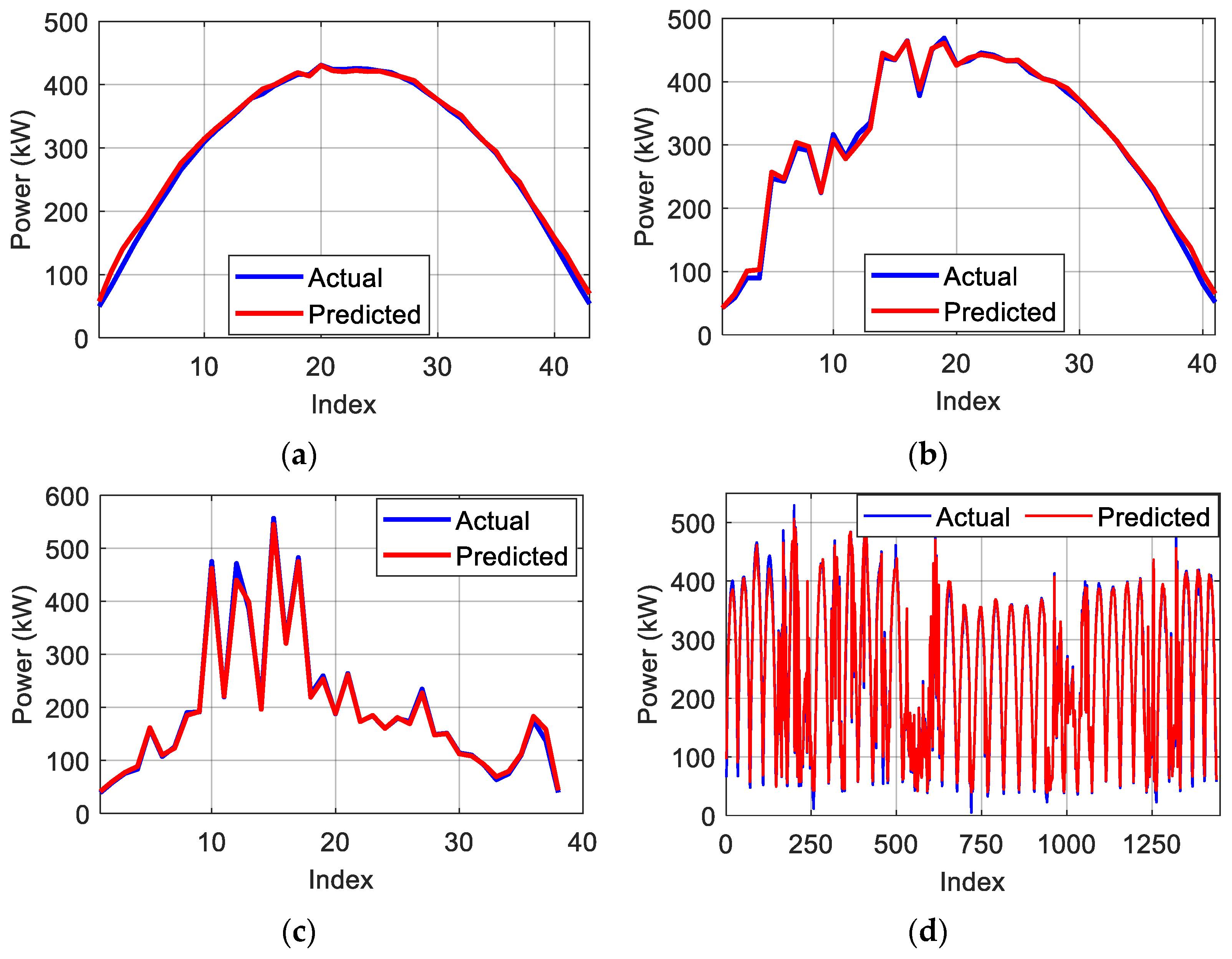
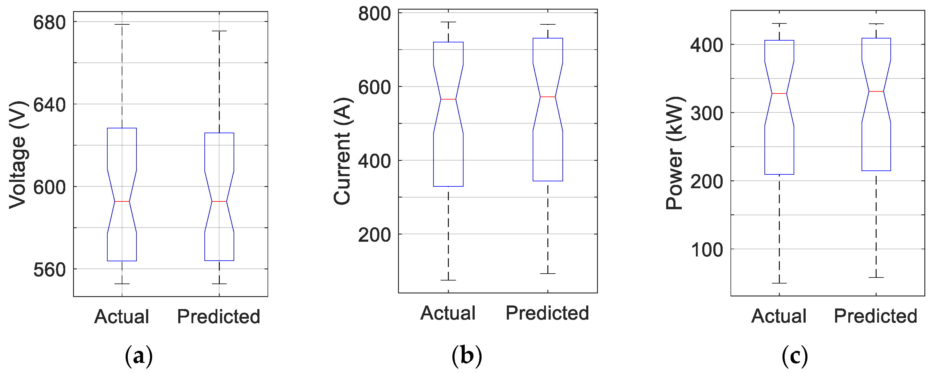
This work has introduced and validated, through experimental measurements, a comprehensive and effective methodology for fault detection and diagnosis of a large-scale PV system by analyzing power losses and two electrical indicators computed using RF and KNN-based prediction models. The proposed models demonstrate reliable predictions of the supplied DC voltage, DC current, and power, making them suitable for fault identification and diagnosis. Indeed, the KNN model successfully predicted the DC voltage, with an R² reaching a value of 0.9967, while the RF model provided reliable predictions for DC current and power, with R² values of approximately 0.9965 and 0.9945, respectively.

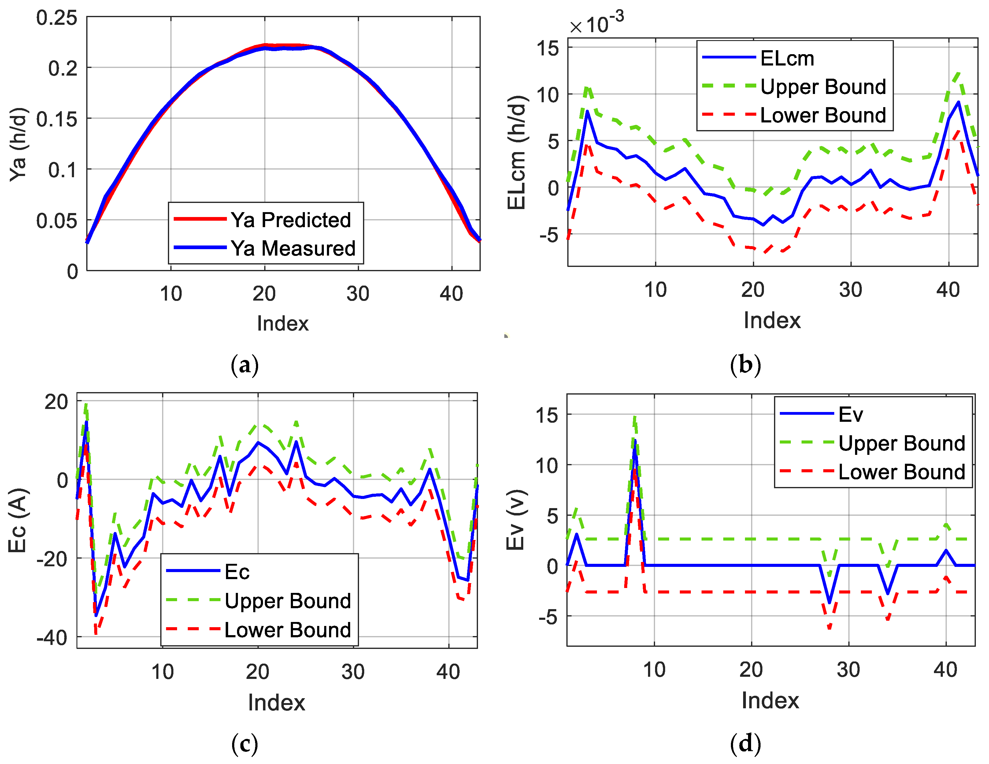
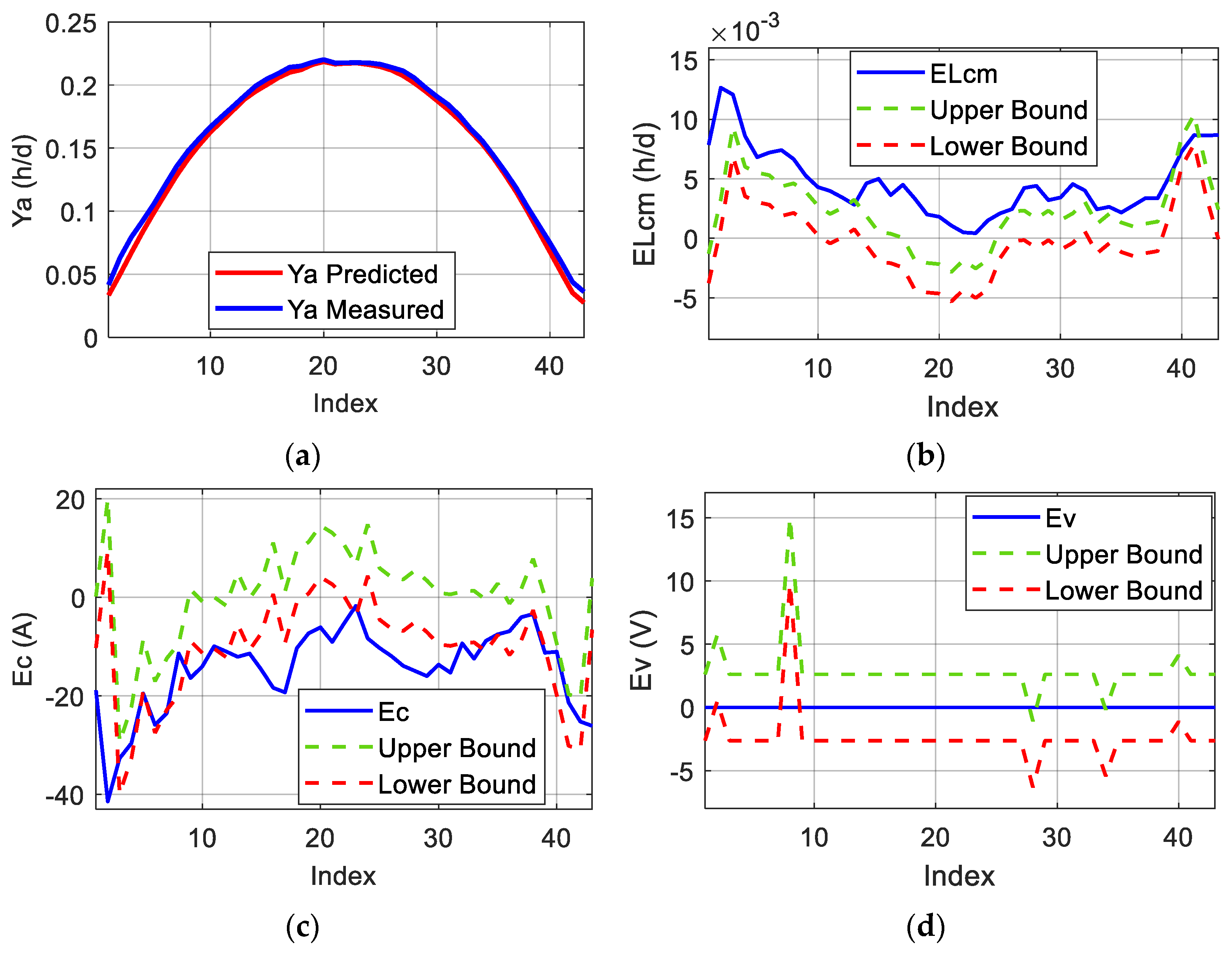
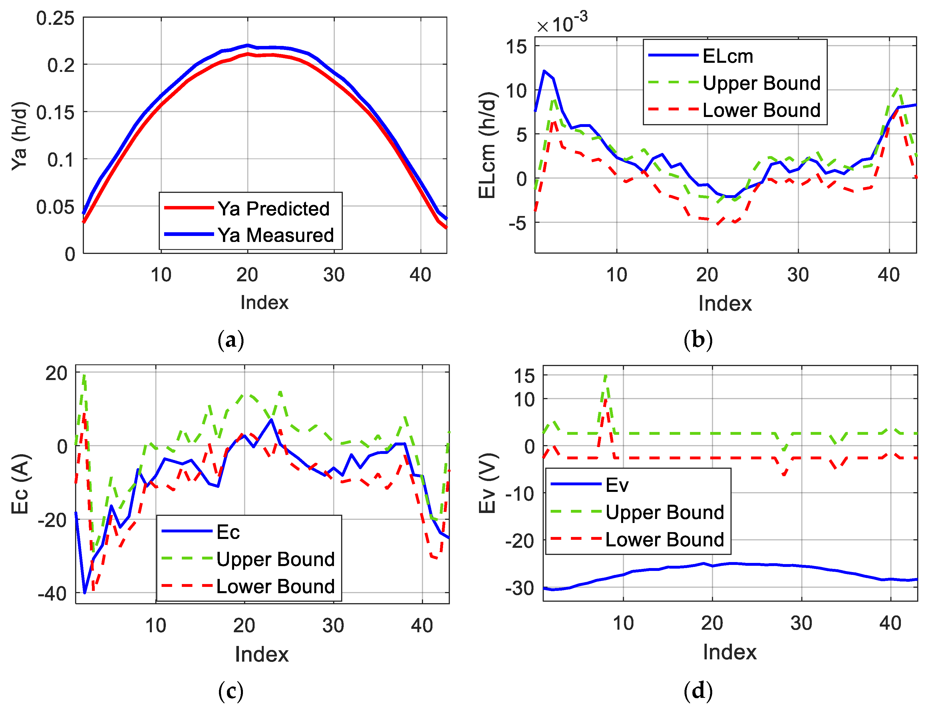
In this context, the miscellaneous capture loss error serves as a key signature for fault detection. A deviation beyond the upper threshold indicates a fault affecting the PV modules, while a deviation below the lower threshold suggests a potentially erroneous measurement from the environmental sensor. Additionally, the signatures of the DC current and voltage errors have been validated for classifying three types of PV faults. Specifically, a deviation in the DC current error beyond predefined thresholds suggests a disconnected string, while a deviation in the DC voltage error is characteristic of a short-circuited module. The final fault pattern, characterized by simultaneous deviations of both voltage and current errors beyond the predefined threshold band, allows for precise classification of a partial shading-induced anomaly.

While it is true that the proposed method does not directly detect Maximum Power Point Tracking (MPPT) errors, which are primarily software-related, their effects still contribute to the overall fault detection process, such as identifying low output power, which may be associated with MPPT inefficiencies.

Future work will focus on refining the proposed methodology to further improve accuracy and adaptability. Integrating deep learning models, such as convolutional and recurrent neural networks, will be explored to enhance fault classification capabilities. Additionally, the deployment of real-time fault detection mechanisms on edge computing platforms will also be considered to enable on-site diagnostics and predictive maintenance. Moreover, implementing adaptive thresholds and self-learning algorithms will be studied to enhance fault detection reliability under varying environmental and operational conditions. Finally, the integration of this system within smart grid infrastructures will be examined to optimize energy management and grid stability.