Detection of Transformer Faults: AI-Supported Machine Learning Application in Sweep Frequency Response Analysis

Abstract

In this study, we discussed how the increasing demand for electrical energy results in higher loads on transformers, creating the need for more effective testing and maintenance methods. Accurate fault classification is essential for the reliable operation of transformers. In this context, Sweep Frequency Response Analysis (SFRA) has emerged as an effective method for detecting potential faults at an early stage by examining the frequency responses of transformers. In this study, we used artificial intelligence (AI) and machine learning (ML) techniques to analyze the data generated by SFRA tests. These tests typically produce large datasets, making manual analysis challenging and prone to human error. AI algorithms offer a solution to this issue by enabling fast and accurate data analysis. In this study, three different transformer conditions were analyzed: a healthy transformer, a transformer with core failure, and a transformer with winding slippage. Six different machine learning algorithms were applied to detect these conditions. Among them, the Gradient Boost Classifier showed the best performance in classifying faults. This algorithm accurately predicted the health status of transformers by learning from large datasets. One of the most important contributions of this study is the use of gradient boosting algorithms for the first time to analyze SFRA test results and facilitate preventive maintenance through the early detection of transformer failures. In conclusion, this study presents an innovative approach. The interpretation of offline SFRA results through various artificial intelligence-based analysis methods will contribute to achieving the ultimate goal of reliable online SFRA applications.

1. Introduction

The technological revolutions that have shaped modern civilization in the last century have resulted from fundamental developments in the fields of communication, transportation, and electrical energy. The achievements of inventors in the fields of communication and transportation have led to the telephone, television, and land and air transport becoming indispensable parts of everyday life. This made it necessary for all countries to rapidly expand their energy infrastructure, including transmission lines, substations, and distribution networks. As a result of these developments, the need for new transformers will increase, and testing and maintenance work will become even more critical due to the additional load on existing transformers. Transformers, devices that enable the widespread use of electrical energy, are invisible but vital to our daily lives [1].

Transformers are classified into various types according to their usage area. Power transformers are one of the most critical components of modern electrical power systems and play a key role in energy transmission and distribution thanks to their high voltage and large power capacities. These transformers enable the transfer of electrical energy from power generation plants to city centers and industrial areas. Power transformers generally operate at voltage levels of 33 kV and above and are designed for large-scale energy transfers. By operating at high voltage levels, they minimize energy losses and make it possible to transmit energy over long distances [2].

Power transformers are among the most expensive types of equipment in electrical power transmission and distribution systems, and monitoring their condition is of great importance for the uninterrupted and reliable operation of the power grid [3]. Power transformers account for up to 60% of the total value of the equipment installed in high-voltage substations [4]. Therefore, techniques for managing the life cycle and monitoring of the condition of power transformers have become increasingly important. These approaches play an important role in reducing maintenance costs and extending the nominal lifetime of transformers.

Transformers undergo testing for various purposes, such as ensuring reliability, performance verification, safety, fault prevention, regulatory compliance, monitoring aging and degradation, installation and commissioning verification, and performance optimization. In this context, tests are of great importance to ensure the reliability of transformers. Since transformers carry high voltages and currents, they must be rigorously tested for compliance with safety standards. These tests evaluate insulation resistance, winding durability, and other safety criteria. Testing also helps prevent serious failures by identifying potential problems in transformers at an early stage. This proactive maintenance approach minimizes downtime and maintenance costs.

Sweep Frequency Response Analysis (SFRA) is a method used to assess the mechanical integrity of the core, windings, and connection structures of power transformers. SFRA is performed by measuring electrical transfer functions over a wide frequency range. These results are compared with the results of other phases of the same transformer. The SFRA process is initiated by sending signals to the transformer at different frequencies. When the transformer is tested at certain frequencies, it produces a unique signature, and this signature is plotted as a curve [5].

The ability to interpret offline SFRA results more reliably with artificial intelligence-supported analysis methods will pave the way for an increase in future studies on online SFRA [6,7].

2. Related Works

In recent years, more studies have been conducted on supporting Sweep Frequency Response Analysis (SFRA) data with artificial intelligence and machine learning techniques in the condition monitoring and fault detection of power transformers. These studies aimed to detect the various mechanical disturbances that occur in transformers more precisely and reliably through different methods. In this section, the main contributions of selected studies from the literature, the methods they used, and how they differ from each other are summarized in a systematic way. In

Table 1. Summary of related works, methods, and contributions.

Related Work	Contribution	Method and Distinction
[8]	Examined the aging of transformers based on field data while also considering potential changes that may occur in SFRA data as a result of this aging.	MATLAB-based Artificial Neural Network (ANN) and Adaptive Network-based Fuzzy Inference Systems (ANFIS) were used in the study.
[5]	Systematically classified the existing studies on the subject into five distinct groups, offering detailed insights into each category, addressed the concept of online SFRA, and presented statistical formulations, including those for the standard deviation and mean.	As a review article, it does not involve any original datasets or empirical analyses derived from experimental procedures.
[9]	Initiated AI-based partial discharge (PD) detection under noisy conditions, laying the groundwork for predictive diagnostics.	Exploited frequency domain FRA signatures and supervised ML models (SVM, RF, 1-D CNN) to localize PD sources with 80–100% accuracy, enabling robust predictive maintenance across diverse transformer states.
[10]	Supplied baseline FRA analyses using classical signal-processing techniques.	Replaces rule-based thresholds with multiple ML classifiers that automatically learn complex FRA patterns, markedly improving fault-detection sensitivity and specificity.
[11]	Investigated forced and free buckling (FDB/FB) faults in windings via FRA.	Extended the fault taxonomy to axial displacement, inter-turn, and combined defects; showed that the trained models generalize across all major winding faults.
[12,13]	Highlighted FRA data scarcity and proposed preliminary processing schemes.	Curates and releases the largest labeled FRA dataset to date; used data augmentation and nested cross-validation to mitigate scarcity and overfitting.
[14]	Focused on disk-space variation (DSV) characterization, giving a targeted view of that single fault type.	Built a comprehensive testbed covering DSV plus radial deformation and tilting, yielding balanced samples for supervised learning and fair comparison.
[15]	Modeled transformer faults in simulation without ML/AI integration.	Combined simulated and measured signatures to train hybrid ML models, delivering the first direct integration of AI into FRA interpretation for transformers.

, the methodological approaches and contributions of important studies in the literature are presented comparatively.

2.1. Contributions

This study makes significant contributions to the field of transformer fault detection by addressing gaps in fault detection methodologies.

• Development of a Novel Fault Detection Framework:

A machine learning-based diagnostic framework for transformer fault classification based on Sweep Frequency Response Analysis (SFRA) data was developed. Multiple classifiers such as Logistic Regression, Random Forest, K-Nearest Neighbor (K-NN), Support Vector Machines (SVMs), Decision Tree, and Gradient Boosting Classifier (GBC) are used.

• Comprehensive Performance Comparison:

Six different machine learning models were systematically compared, and the Gradient Boosting Classifier showed superior performance in terms of accuracy, precision, recall, and F1 score.

• Experimental Validation in Real Failure Scenarios:

Experimental validation studies with SFRA data obtained from transformers with core failure and winding displacement demonstrate the applicability of the proposed system in real field conditions.

• Advanced Data Analysis and Visualization:

The model’s performance was comprehensively evaluated using not only basic accuracy measures but also multidimensional analysis tools such as confusion matrices, learning curves, calibration curves, gain plots, and Kolmogorov–Smirnov (KS) statistics.

• User Interface Development for Practical Use:

With the (GUI) developed using Python’s Tkinter library, it is possible for users without programming knowledge to perform transformer condition monitoring and fault prediction.

2.2. Novelty

This study has been developed by considering gaps in the literature and brings a new perspective to transformer fault diagnosis.

• First Application of GBC for Multi-Class Transformer Fault Diagnosis:

The Gradient Boosting Classifier (GBC) was applied for the first time to diagnose different fault categories (core fault and winding displacement) using SFRA data.

• Comprehensive Comparison Among Various Machine Learning Methods:

This is a rare study that comprehensively compares Logistic Regression, Random Forest, K-NN, SVC, Decision Tree, and GBC methods for SFRA-based transformer fault detection.

• Frequency-Independent Classification Performance:

The trained models are able to perform fault detection with high accuracy without being bound to specific frequency ranges, thus demonstrating frequency-independent diagnostic capability.

• Detailed and Structured Dataset Generation:

A comprehensive dataset containing both amplitude and phase information in multiple phases (U1, V1, and W1) was created, labeled, and used for model training. This dataset is an important resource for future studies.

In this study, we focused on diagnosing transformer fault conditions using artificial intelligence and machine learning algorithms, particularly through the analysis of Sweep Frequency Response Analysis (SFRA) tests. The article is organized into several sections to provide a clear and structured approach. The third section, titled Materials and Methods, offers an in-depth explanation of the mathematical principles underlying transformer operations, as well as the methods used in transformer testing, with a particular focus on the SFRA test. In addition, the artificial intelligence algorithms used in this study are introduced, with special attention given to the Gradient Boosting Classifier (GBC), which provided the best results. The practical implementation of the methodology, including the processes of data collection, preprocessing, and modeling, is thoroughly outlined. The Research Findings and Discussion sections evaluate the performance of the proposed models, showcasing key results through various evaluation metrics. The Results section summarizes the key findings of the study, emphasizing their impact on transformer fault diagnosis and potential applications. This structure is designed to enhance the clarity and comprehensiveness of the study for the reader.

3. Materials and Methods

This section provides theoretical insights into mathematical calculations for transformers, various transformer tests, and particularly the SFRA (Sweep Frequency Response Analysis) test. Detailed explanations are included regarding the nature of SFRA tests, procedures for conducting these tests, and interpretation of results using Bode diagrams. Subsequently, the artificial intelligence algorithms employed in this study are introduced, with a specific emphasis on the gradient boosting algorithm, which yielded the most successful results. Finally, the practical implementation phase of this study is thoroughly detailed under this section, offering a comprehensive explanation of the applied methodology.

3.1. Transformers and Mathematical Methods of Study

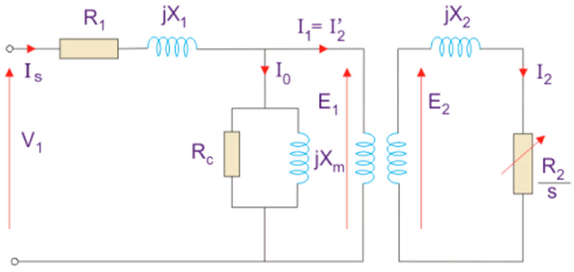
Transformers are electromechanical devices that convert electrical energy from one voltage level to another. According to the IEC 60076-1 [16], transformers are static devices that convert alternating current and voltage systems into different values by electromagnetic induction. Although all transformers differ according to their intended use, their operating principles are the same [17]. Figure 1 illustrates the equivalent circuit model facilitates transformer analysis and performance evaluation. Transformers consist of two main components: the magnetic core and the winding. The magnetic core drives the magnetic flux, while the windings provide the induction of electric current. When alternating current is applied to the primary winding, it produces a magnetic flux that is conducted from the core to the secondary winding, inducing output voltage. The operating principle of transformers is based on Faraday’s law of electromagnetic induction.

3.2. Transformer Testing

Before transformers are accepted for operation, a series of comprehensive tests are conducted. These tests assess the condition of insulation materials, the appropriateness of winding connections, the maintenance of the core’s position, changes in the insulation distance between the windings and the ground, the detection of possible breaks in the windings, the evaluation of short-circuit probabilities in the winding turns, and the status of the tap changer. This paper particularly focused on the SFRA test.

3.3. Sweep Frequency Response Analysis (SFRA)

The Sweep Frequency Response Analysis test is one of the most critical tests that must be performed during factory acceptance and field operations. It is a parameter obtained by applying a terminal voltage source across two terminals of the test object at different frequency ranges and measuring the amplitude ratio and phase angle. The SFRA technique evaluates the test results by using data obtained from the frequency response to detect damage. In this context, SFRA tests are vital for the early detection and monitoring of potential damage in transformers. 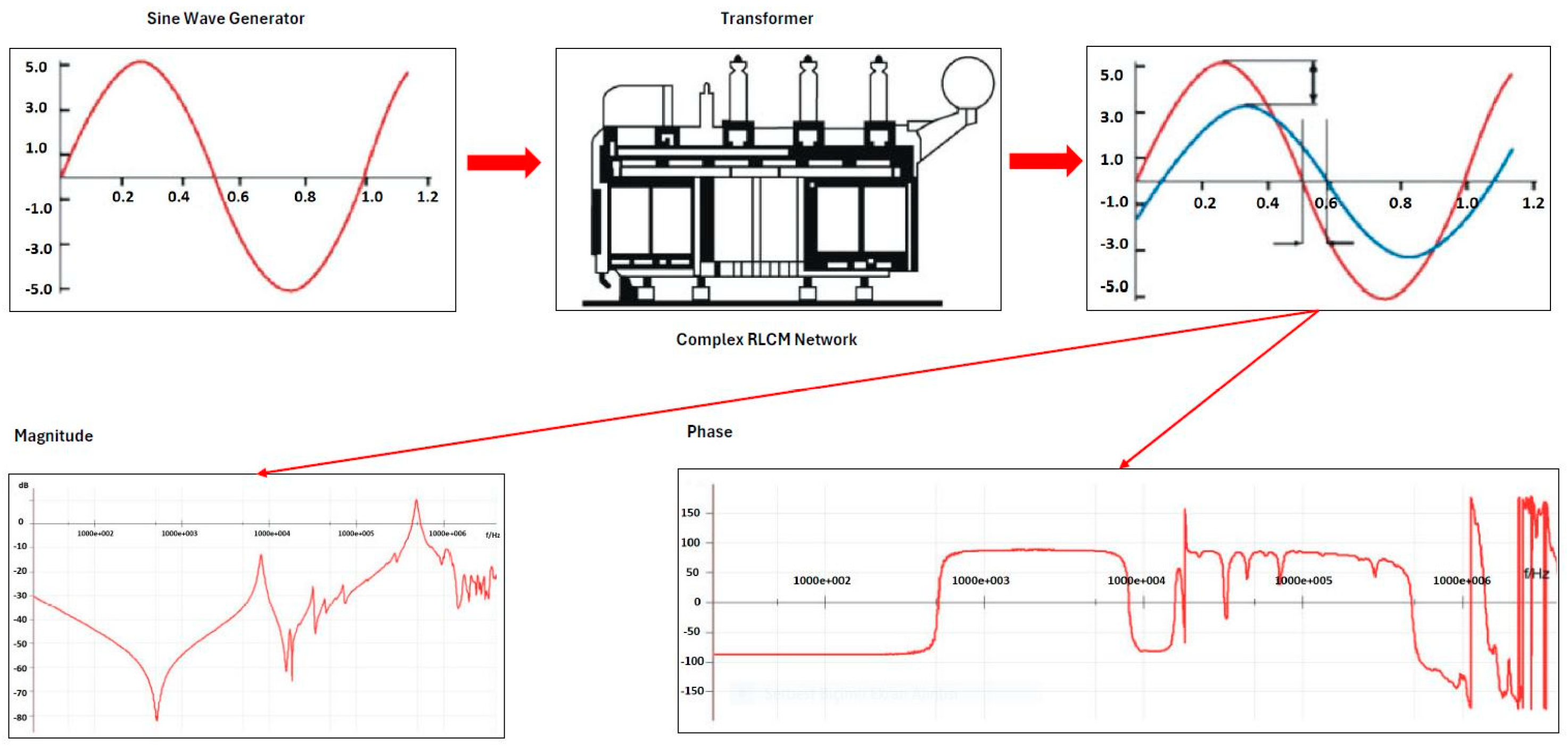The developed standards and methodologies increase the reliability and effectiveness of SFRA tests, contributing to the safer and more sustainable operation of power systems [18,19]. The basic principle of SFRA tests works by applying an under-voltage signal to one terminal of the transformer and measuring it from the other, as explained in the general principle diagram shown in Figure 2. These measurements are made in decibels (dB) and repeated at all terminals of the transformer. The data obtained are used to assess the mechanical and electrical condition of the transformer.

SFRA analyzes the response of components, such as resistance (R), inductance (L), and capacitance (C), in electrical circuits to changes in frequency. The SFRA of transformer windings shows significant resonances at low frequencies. These resonances are caused by the frequency-dependent response of inductive and capacitive components in the circuit. SFRA is used to detect possible faults by analyzing the frequency response of transformers.

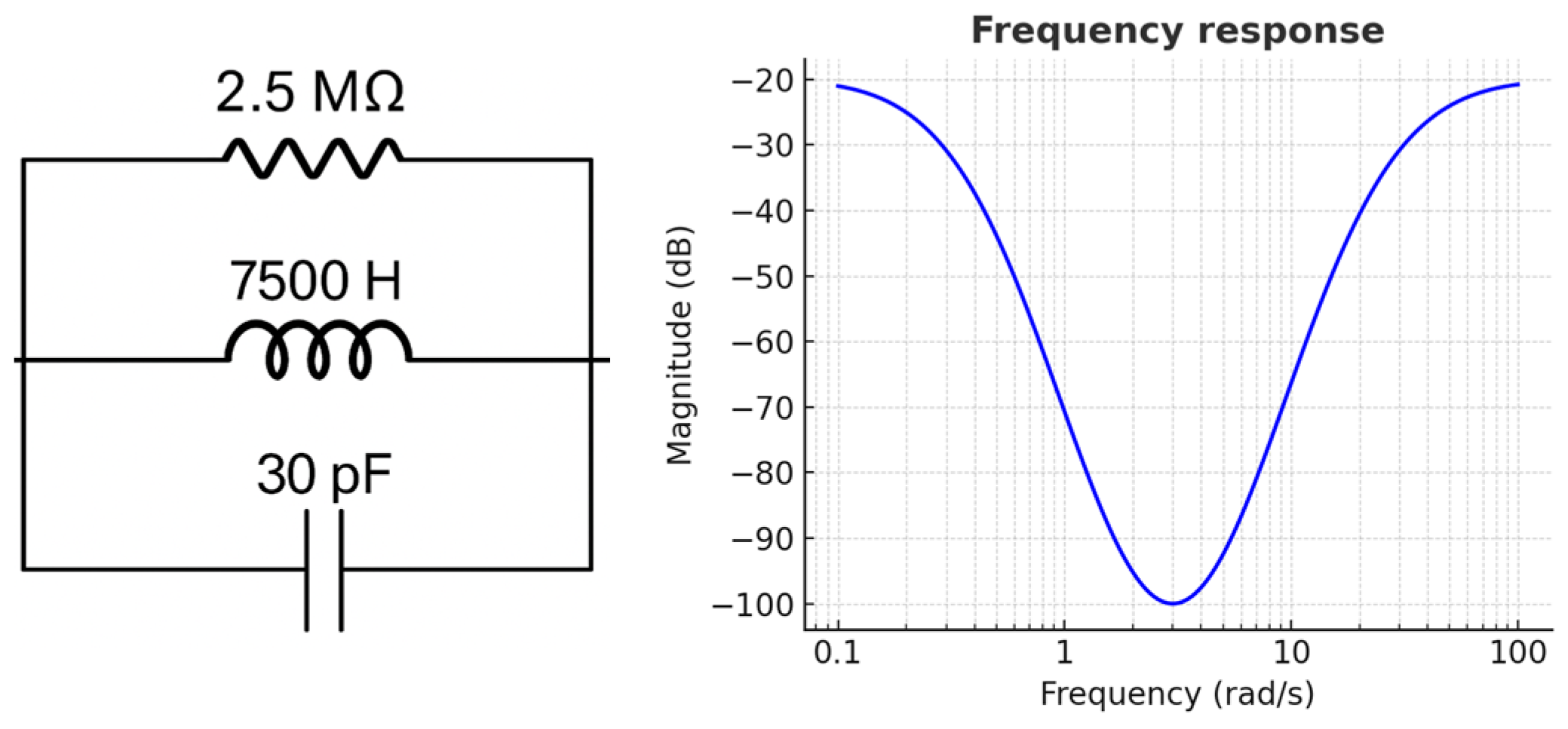
The RLC circuit example in Figure 3 and the frequency response plot in logarithmic scale provide a visual representation of the resonance points and their variations in the circuit. These graphs obtained in SFRA are important for understanding and interpreting the characteristic responses of the device, obtaining information about its performance and performing preventive maintenance by early detection of possible faults. The system response can be analyzed in both time and frequency domains, and techniques such as frequency response analysis (FRA) are used in this analysis. Various mathematical tools and techniques are available to analyze system responses. While differential equations or convolution are used in the time domain, Fourier and Laplace transforms are preferred in the frequency domain. These transforms allow the system to switch between time and frequency domains. SFRA is one of the application areas of these transforms. A function in the time domain is moved to the frequency domain by Fourier transform and analyzed through its frequency components. In this transformation, the function f(t) in the time domain becomes F(jω) in the frequency domain. With the inverse Fourier transform, the function F(jω) can be returned to the time domain as f(t). This mathematical relationship plays a critical role in understanding the response of the system in both time and frequency domains (Equation (1)).

$$F(j\omega )={\int }_{-\infty }^{\infty }{e}^{-j\omega t}f(t)dt>f\left(t\right)={\displaystyle \frac{1}{2\pi }}{\int }_{-\infty }^{\infty }{e}^{-j\omega t}f\left(j\omega \right)d\omega$$

$$F\left(t\right)+N\left(t\right)={\displaystyle \frac{1}{2\pi }}{\int }_{-\infty }^{\infty }{e}^{-j\omega t} f\left(t\right)dt \left[F\left(j\omega \right)+N\left(j\omega \right)\right]d\omega$$

(1)

$$F\left(t\right)=\mathrm{Orginal} \mathrm{Signal},\hspace{1em}\hspace{1em}N\left(t\right)=Noise$$

Analyzing the system response in the time domain is difficult, especially in complex electrical systems. However, analyses in the frequency domain are more suitable to overcome these difficulties. In the frequency domain, analyzing different frequency components provides a clearer understanding of the characteristics of the system such as amplitude and phase. Different frequency components with the same impedance value can be examined, and effects such as unwanted noise and harmonics in the system can be analyzed more easily. The transfer function (Equation (2)) describes the relationship between the inputs and outputs of a system in the frequency domain and determines the amplitude and phase changes. The roots of this function form the zeros and poles of the system and are important for understanding the dynamic behavior of the system.

$$H(j\omega )={\displaystyle \frac{V_{output\left(j\omega \right)}}{V_{input\left(j\omega \right)}}}$$

(2)

Because 50 Ω impedance is used as standard in SFRA devices, SFRA measurements calculate the transfer function using voltage ratios. Equations (3) and (4) form the mathematical basis of the Bode diagram. These equations allow the amplitude and phase to be calculated as a function of frequency using the transfer function of the system (H(jω)). These calculations are used to draw the Bode diagram, which is an important tool in analyzing the frequency response of RLC circuits and transformers. The Bode diagram shows the variation in amplitude and phase with frequency using the transfer function of the system. The use of a logarithmic scale allows a clearer visualization of the dynamic behavior of the system over a wide frequency range. Zeros and poles cause 20 dB changes in the Bode diagram, which are important for analyzing the resonance and stability of the system.

$$A\left(dB\right)=20{log}_{10}\left(H\left(j\omega \right)\right)$$

(3)

$$A\left(\theta \right)={\tan }^{-1}\left(H\left(j\omega \right)\right)$$

(4)

The logarithmic scale allows changes in low and high frequencies to be shown on a single graph. This is an important advantage compared to linear scale graphs, which cannot show the variations at high frequencies clearly enough. SFRA measurements for transformer fault detection are not limited to a single measurement but include different connection types and methods. In this way, various types of faults can be detected and compared with previous measurements. All variations in previous measurements must be recorded and analyzed to correctly detect faults that occur over time.

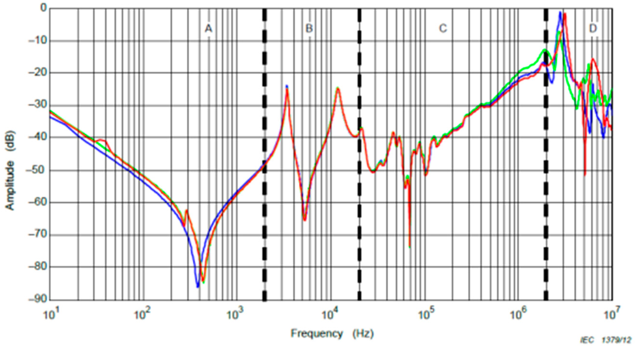
SFRA analyzes fingerprints of the transformer by determining its characteristic frequency response. This unique frequency response represents the condition of the transformer at a given time and is used as a reference point for future routine checks. By detecting even the smallest changes that may occur in the transformer over time, SFRA enables early diagnosis of mechanical or electrical faults. This way, maintenance processes are optimized and the life of the transformer is extended. Turkish Electricity Transmission Co. Ankara, Turkiye (TEIAS) uses the graph given in Figure 4 as the SFRA evaluation graph.

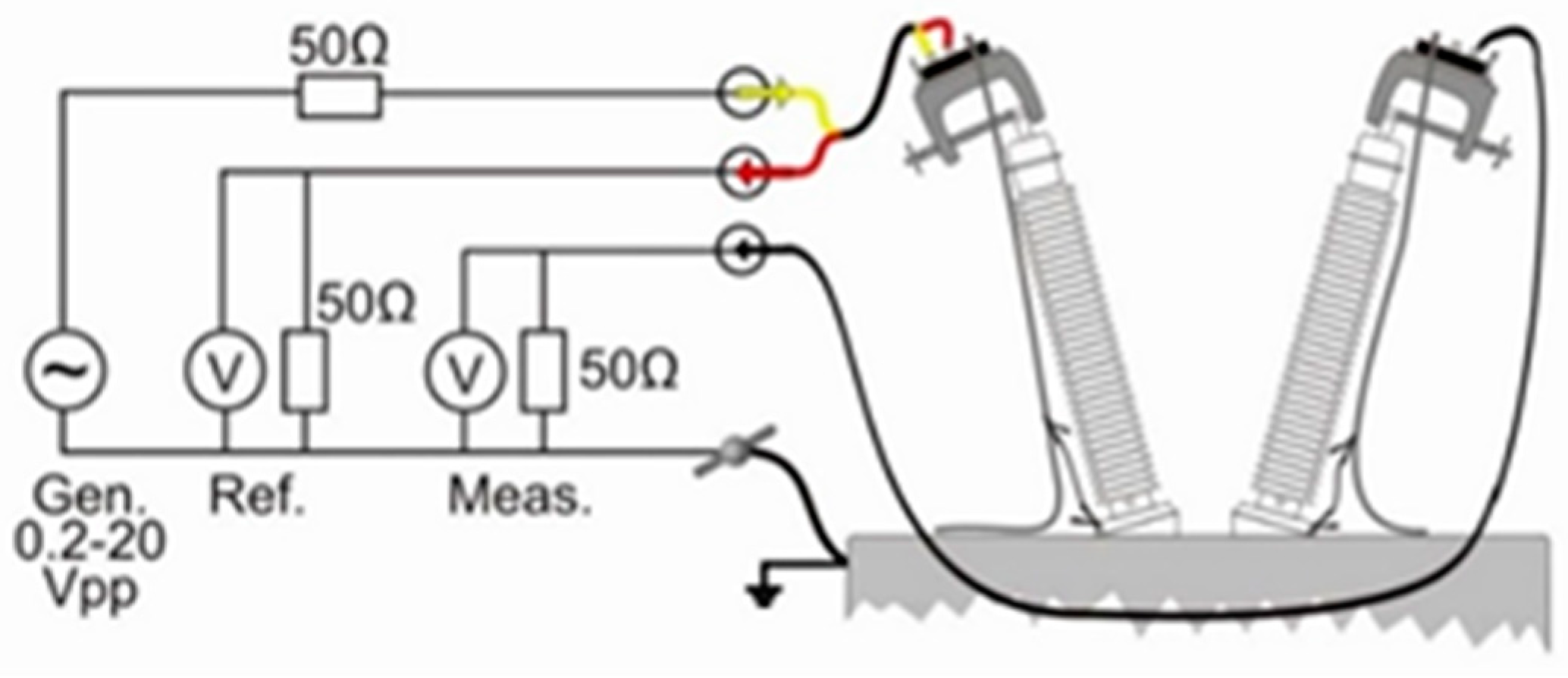
SFRA measurements use various connection scenarios to evaluate different characteristics of the transformer. The basic measurements are winding-end-to-winding-end and inter-winding capacitive and inductive measurements. Winding-end-to-winding-end measurements are performed under open- and short-circuit conditions. Capacitive measurement analyzes inter-winding capacitance, and inductive measurement analyzes magnetic interactions. Measurements can also be made at the source phase of the transformer or at the neutral terminal to examine different phase combinations. In short-circuit tests, each phase can be measured separately, or all phases can be short-circuited together. The basic measurement principle diagram of frequency response analysis is shown in Figure 5.

3.4. Artificial Intelligence and Machine Learning Techniques

Machine learning is a branch of artificial intelligence that enhances the ability of computer systems to learn from data and make predictions without explicit programming. In this study, various machine learning techniques—such as logistic regression, K-Nearest Neighbors (K-NN), Support Vector Classifier (SVC), decision trees, and gradient boosting—were individually tested and evaluated based on their performance outcomes. Logistic regression is a widely used statistical modeling technique for binary classification problems; it models the relationship between independent variables and a dependent variable. K-Nearest Neighbors (K-NN) is an algorithm that determines the class or value of a data point by examining the classes or values of its K-Nearest Neighbors [21]. Support Vector Classifier (SVC) is a flexible and robust algorithm frequently applied in classification problems. It projects the data into a high-dimensional space to find the optimal separation between two classes [22]. Decision trees split data into branches and leaves based on a set of decision rules for classification [23]. Gradient Boosting Classifier (GBC) is a powerful ensemble learning method. It sequentially trains a series of weak learners (decision trees) to form a strong learner. Each tree aims to correct the errors of its predecessor. As the number of labels increases, so does the number of trees, allowing the model to gradually address previous errors [24]. These machine learning techniques have been applied individually to the SFRA test results of transformers for fault detection. As shown in

Table 2. Comparative overview of machine learning methods applied in transformer fault diagnosis.

Machine Learning Method	Advantages	Disadvantages
Logistic Regression (Lr)	Simple and fast implementation; effective for binary classification problems.	Limited performance for complex or multi-class classification tasks.
Random Forest Classifier (Rf)	Robust against overfitting; achieves high classification accuracy.	Difficult to interpret; may require substantial memory and computational resources.
K-Nearest Neighbors (K-Nn)	Non-parametric; provides intuitive classification based on proximity.	Computationally expensive for large datasets; sensitive to noise and irrelevant features.
Support Vector Classifier (Svc)	Effective in high-dimensional spaces; forms robust decision boundaries.	Computationally intensive for large-scale datasets; sensitive to choice of kernel parameters.
Decision Tree Classifier (Dt)	Easy to interpret and visualize; fast training and prediction phases.	Prone to overfitting, particularly with small datasets or when not properly pruned.
Gradient Boosting Classifier (Gbc)	High prediction accuracy; sequentially corrects errors of weak learners to form a strong model.	Requires careful parameter tuning; relatively long training time.

, a comparative overview of machine learning methods applied in transformer fault diagnosis highlights the advantages and disadvantages of various algorithms, which can guide the selection of the most suitable method based on the specific requirements of the fault detection task.

3.5. Data Processing, Modeling, and Visualization Processes in Fault Detection

In this study, the selection of classification algorithms was based on the nature of the data and the practical requirements of the problem. The Sweep Frequency Response Analysis (SFRA) data are characterized by a tabular, low-dimensional numerical structure rather than image-like or sequential dependencies. Therefore, classical machine learning algorithms such as Logistic Regression, Random Forest, K-Nearest Neighbors (K-NN), Support Vector Classifier (SVC), Decision Trees, and Gradient Boosting Classifier (GBC) were deemed more appropriate in terms of training efficiency, interpretability, and operational practicality. Specifically, although XGBoost 3.0.0 is a powerful gradient boosting technique, it requires extensive hyperparameter tuning and computational resources. Since the Gradient Boosting Classifier (GBC) already achieved high classification performance in this study, the additional complexity introduced by XGBoost was considered unnecessary within the scope of this work. Convolutional Neural Networks (CNNs) are primarily effective on spatially correlated data such as images or structured signal representations. SFRA data do not possess inherent two-dimensional spatial structures; thus, applying CNN architectures would introduce unjustified complexity without a corresponding performance gain. While more complex architectures could be explored in future studies, this study intentionally prioritized maximum classification performance with minimum model complexity.

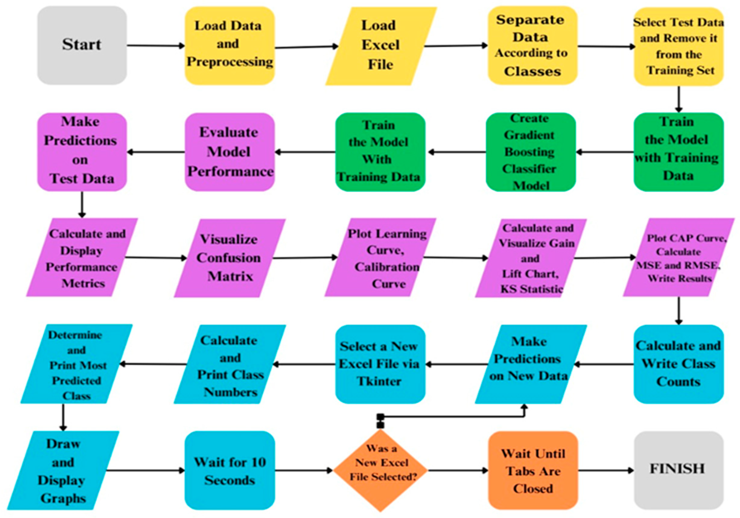
At the beginning of the study, the data obtained from the test transformer, where core short circuits and winding shifts were created, were subjected to data loading and preprocessing stages using Sweep Frequency Response Analysis (SFRA). In this phase, the raw data were cleaned and made suitable for analysis. Subsequently, the data were loaded in Excel format and categorized according to classes. The separation of training and test data is a critical step for evaluating the model’s performance and was implemented as a strategy to prevent overfitting. The study was ultimately completed using the Gradient Boosting Classifier algorithm, which exhibited the best performance during the model training process. The model learned patterns within the dataset by being trained with the training data. After completing the model training, predictions were made on the test data, and the model’s performance was evaluated. During the performance evaluation, various metrics (such as confusion matrix, accuracy, precision, recall, etc.) were calculated and reported for a detailed analysis of model performance, the confusion matrix was calculated and visualized. Learning curves and calibration curves were plotted to examine the model’s learning capacity and calibration. Additionally, the effectiveness and discriminative power of the model were assessed using gain and lift charts, along with KS statistics. Furthermore, the CAP curve was plotted, and the mean squared error (MSE) and root mean squared error (RMSE) values were calculated to measure the model’s errors. The model’s generalization capability was tested by making predictions on new data. During the analysis of the prediction results, the predicted class was identified and reported. The class distribution was calculated to determine which class the model showed a higher tendency toward. Visualizing the analyses is crucial for making the results obtained more comprehensible. To facilitate user interaction, a graphical user interface (GUI) was created using the Tkinter library. Through this interface, users can select a new Excel file to repeat the processes.

Upon completion of the process, the results were obtained and reported. This structure comprehensively addresses critical steps such as data processing, model building, performance evaluation, and result visualization. This approach ensures that the study is conducted systematically and scientifically. The flow diagram of the study is presented in Figure 6.

3.6. Data Collection and Dataset Creation

The Sweep Frequency Response Analysis (SFRA) measures the response characteristics of a transformer at various frequencies to detect potential deformations in its internal structure, winding displacements, insulation issues, and other structural anomalies. The application of the SFRA follows a specific procedure. The test transformer was deliberately engineered to permit controlled displacement of the windings and the introduction of core faults. Consequently, the test protocol involved the execution of thousands of experiments, primarily targeting the most frequently encountered transformer defects, specifically axial and radial winding displacements and core anomalies. After the testing equipment is set up, a signal is sent to the transformer within a specific frequency range typically between 20 Hz and 2 MHz, see Figure 7. During this frequency sweep, the frequency response of the transformer is recorded and analyzed. The obtained data are compared with reference data or previous test results to assess the mechanical and electrical integrity of the transformer. For this study, the test setup was implemented using the Omicron FRAnalyzer, Omicron electronics GmbH, Klaus, Austria, with software version V 2.2.180. This device plays a crucial role in providing accurate frequency response measurements, making it an essential tool for investigating the internal structure of transformers. The application of this technology in fault detection has been thoroughly explored and discussed in the context of this study.

The SFRA results are visualized using Bode diagrams, which consist of two components that represent the frequency response of a system: magnitude and phase plots. In the magnitude plot, frequency is displayed on the horizontal axis, and magnitude is shown on the vertical axis. Frequency is typically expressed on a logarithmic scale, and magnitude is represented in decibels (dB). These Bode diagrams allow for the early detection of potential issues within the internal structure of the transformer, enabling preventive maintenance to be conducted. The obtained data are compared with reference data or prior test results to evaluate the mechanical and electrical integrity of the transformer.

3.7. Data Preprocessing and Dataset Creation

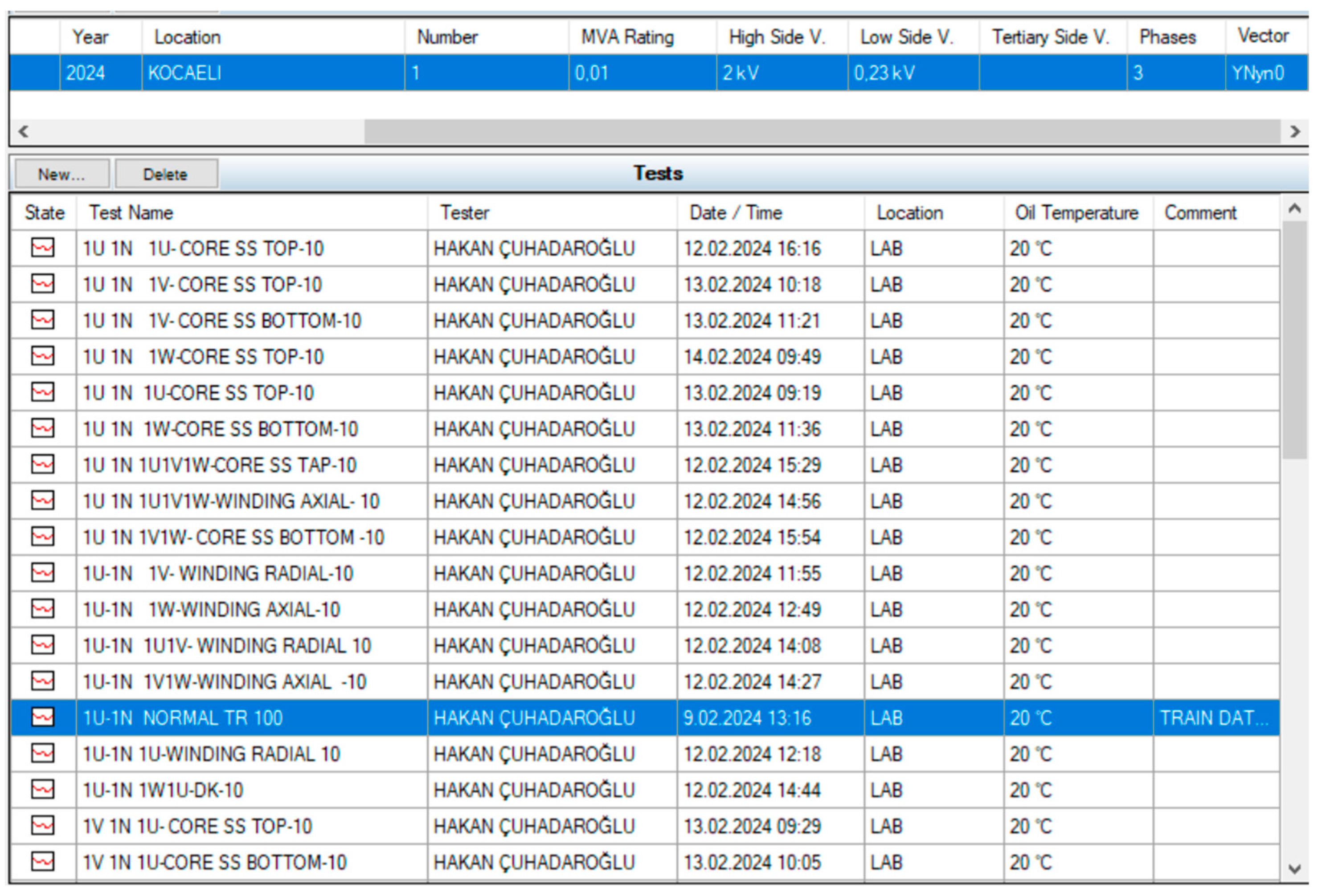
The dataset used in this study contains data corresponding to the U1, V1, and W1 phases. These data include winding shift and core faults for each phase with a neutral connection, as well as data pertaining to healthy operating conditions. The data encompass measurements at the lower and upper connection points for each phase and fault type. This comprehensive dataset allows for the analysis of how each phase behaves under different types of faults while also providing the opportunity for comparison with healthy conditions. Thus, it becomes possible to examine the frequency responses of healthy connections, as well as winding shift and core faults at the lower and upper connection points. The dataset used in the software consists of a total of 481,000 rows and 4 columns. The first column contains frequency values, the second column contains magnitude values, and the third column includes phase values. The fourth column contains the labeled versions of the data: healthy data are labeled as 0, data with core faults as 1, and data with winding shift faults as 2. In artificial intelligence studies, class labels are denoted as 0-1-2. This labeling facilitates the analysis of the data with machine learning models and enables classification. Letters and other meaningless data were excluded, allowing the dataset to be processed according to specific parameters and made suitable for classification. Sixty percent of the dataset was allocated for training, while forty percent was reserved for testing. As shown in Figure 8, various tests were conducted on the transformer under different configurations.

3.8. Tools and Software Used

In this study, Python 3.12 was utilized as the programming language for machine learning. Python and its libraries provide a powerful, flexible, and user-friendly toolkit highly suited for machine learning and artificial intelligence applications. In this work, Python libraries (pandas 2.2.2, matplotlib 3.8.4, seaborn0.13.2, scikit learn1.4.2, tkinter, numpy 1.26.4, time, sklearn, calibration) were effectively employed for these applications. Pandas facilitated speed and flexibility in data analysis, while matplotlib and seaborn were used to create esthetically pleasing and detailed visualizations of the data. Scikit learn included robust machine learning algorithms, simplifying the modeling and performance evaluation processes and enabling the implementation of complex algorithms such as the Gradient Boosting Classifier. Tkinter offered a user-friendly interface for easily monitoring model results, and numpy provided efficiency in numerical computations. The time library was used to optimize the execution times of the code, while sklearn calibration calibrated the model for accuracy and reliability, allowing for more accurate predictions. With the aid of these libraries, the project was completed in the most efficient manner, enabling the rapid, reliable, and effective processing of complex datasets and models.

In this study, PyCharm version 2023.1.3 was used. PyCharm is an integrated development environment (IDE) optimized for the Python programming language and developed by JetBrains. It provides a highly suitable development environment for artificial intelligence and machine learning projects.

4. Research Findings

In this study, six machine learning algorithms were investigated: logistic regression, Random Forest, K-Nearest Neighbors (K-NN), Support Vector Classifier (SVC), decision trees, and Gradient Boosting Classifier (GBC). Based on the performance outcomes, the “Gradient Boosting Classifier” algorithm was selected. The Gradient Boosting Classifier algorithm yielded the most successful results among the other machine learning techniques tested on the dataset. An additional significant feature of the Gradient Boosting Classifier (GBC) method is its superior performance not only in binary metrics but also in multi-class metrics. Given that there are three different label values in this study, the Gradient Boosting Classifier (GBC) method achieved more successful outcomes. The performance results of the algorithms are presented in

Table 3. Performance results of different models.

Performance Results Table	Accuracy	Precision	Recall	F1 Score
Logistic Regression	0.7768	0.7996	0.7927	0.7924
Random Forest Classifier	0.8868	0.8928	0.8815	0.8522
K-Nearest Neighbors	0.6941	0.6635	0.6814	0.6855
Support Vector Classifier	0.8569	0.8535	0.8911	0.8552
Decision Tree Classifier	0.7961	0.7954	0.7740	0.7813
Gradient Boosting Classifier	0.9142	0.9205	0.9142	0.9141

.

In this study, six different machine learning classification algorithms were tested using transformer data obtained from SFRA tests to perform fault detection, and four fundamental metrics were used to evaluate their performance: overall accuracy, overall precision, overall recall, and overall F1 score. These metrics are critical indicators that provide a comprehensive assessment of a model’s success in machine learning studies. Overall accuracy refers to the ratio of the number of correctly predicted instances to the total number of instances. It indicates the model’s capacity for accurate predictions for both positive and negative classes. In this study, the highest accuracy value of 0.9142 was achieved with the Gradient Boosting Classifier (GBC) algorithm. Overall precision measures how many of the instances predicted as positive by the model are positive. This metric aims to reduce the rate of false positives and is particularly important in situations where false positives carry significant costs. The highest precision value of 0.9205 was also achieved with the GBC algorithm. Overall recall indicates the rate at which the model accurately captures actual positive instances. This metric aims to reduce the rate of false negatives and is crucial in scenarios where it is essential for the model to not miss true positives. The highest recall value of 0.9142 was calculated with the GBC algorithm in this study. Overall F1 score presents the harmonic meaning of the precision and recall metrics. It is considered a reliable performance measure, especially for datasets with class imbalance. The F1 score balances the model’s ability to capture positive classes with high accuracy and its capacity to avoid false positive predictions. In this study, the highest F1 score of 0.9141 was obtained with the GBC algorithm. In conclusion, when comparing the performance metrics of the six different algorithms, the Gradient Boosting Classifier (GBC) model provided the best results and was determined to be the most suitable model for the paper.

4.1. Evaluation of Model Performance

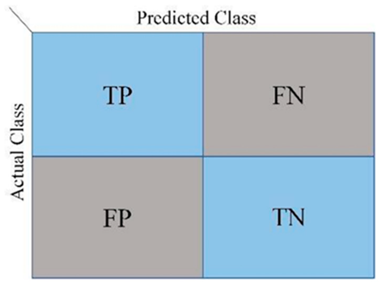
The confusion matrix is a fundamental and critical tool used to evaluate the performance of classification models in machine learning and statistics. This matrix visually presents the relationship between the classes predicted by the model and the actual classes, allowing for a detailed analysis of classification performance. An example structure of the confusion matrix is provided in Figure 9. It is vital to identifying where the model has made errors and to understanding the nature of these errors in imbalanced datasets. In binary classification problems, the confusion matrix consists of four main components: true positives (TPs), true negatives (TNs), false positives (FPs), and false negatives (FNs). These components enable the calculation of various performance metrics, such as accuracy (Equation (5)), precision (Equation (6)), and recall (Equation (7)).

$${\displaystyle \frac{TP+TN}{TP+TN+FP+FN}}$$

(5)

$${\displaystyle \frac{TP}{TP+FP}}$$

(6)

$${\displaystyle \frac{TP}{TP+FN}}$$

(7)

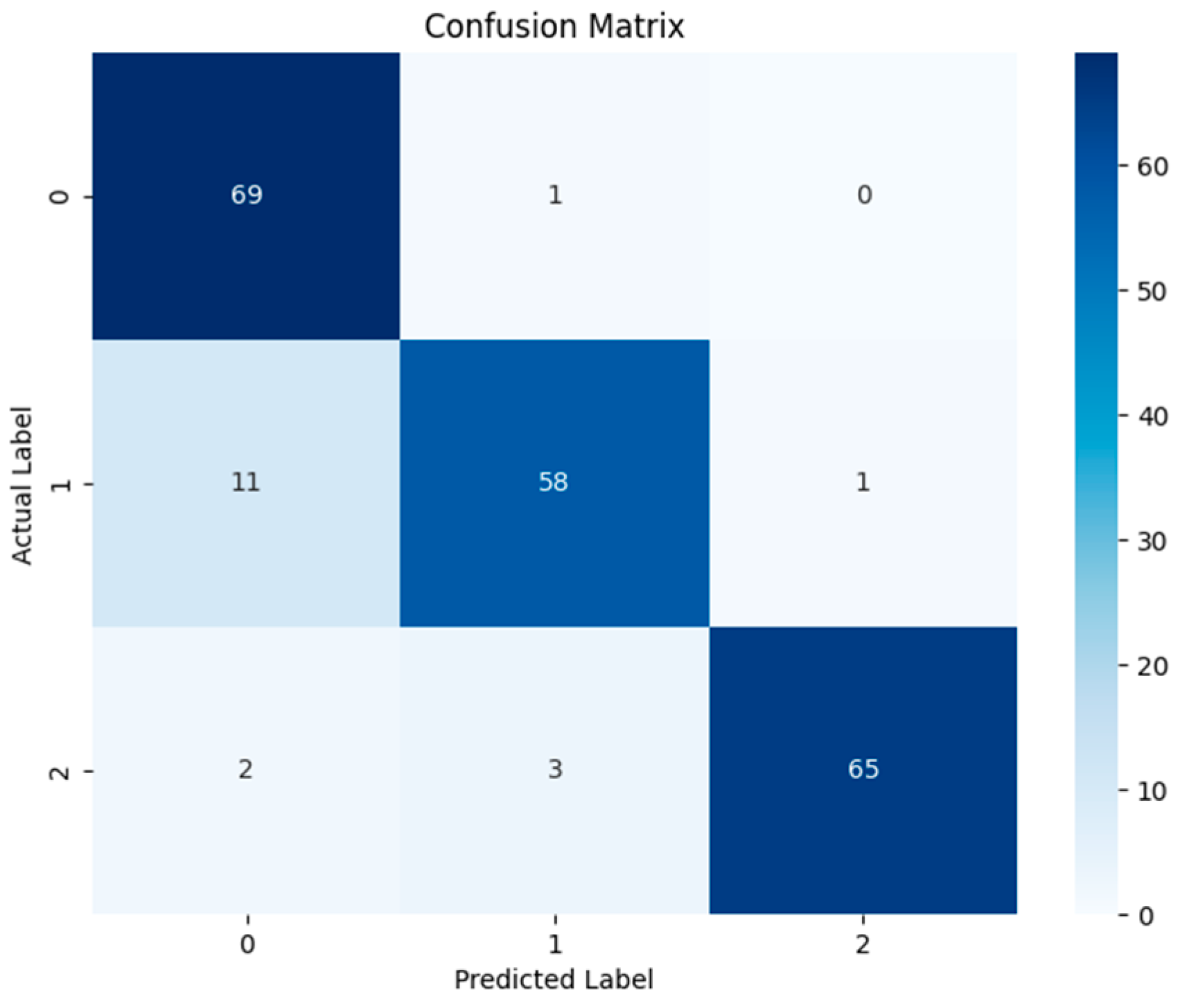
The confusion matrix can also be widely used in multi-class and multilabel classification problems. The matrix size for multi-class problems is n × n, where n represents the number of classes. In such matrices, each cell indicates how many times where actual instances belonging to a given class are predicted as another class. In multilabel classifications, each instance may have more than one label, and the confusion matrix can be generalized to account for this situation as well. Overall accuracy can be misleading with imbalanced datasets, but the confusion matrix provides separate performance metrics for each class. Furthermore, understanding which types of errors (false positives or false negatives) are more common provides important insights into how the model can be improved. In this study, there are three classes: healthy data, winding displacement errors, and core errors. The performance of the algorithm with the highest accuracy (Gradient Boosting Classifier, GBC) is evaluated using the confusion matrix. The confusion matrix for the outputs of this study is presented in Figure 10.

Each cell of the confusion matrix indicates the counts of correct and incorrect classifications made by the model. For healthy data (Class 0), out of 70 data points, 69 were correctly classified, with only 1 misclassified as a winding shift fault. For winding shift faults (Class 1), 58 out of 70 data points were correctly classified, while 11 were incorrectly classified as healthy data and 1 as core fault. In the case of core faults (Class 2), 65 out of 70 data points were correctly classified, with 2 incorrectly classified as healthy data and 3 as winding shift faults. The overall accuracy of the model was calculated as the ratio of all correct classifications to the total number of classifications, yielding an approximate accuracy of 91.4%. Precision and recall rates were also evaluated on a class-by-class basis. For healthy data, the precision was 85 and the recall was 98.6%. For winding shift faults, the precision was 93.6% and the recall was 82.9%. For core faults, the precision was 92.9% and the recall was 92.8%.

4.2. Performance Evaluation Graphs Obtained from the Paper

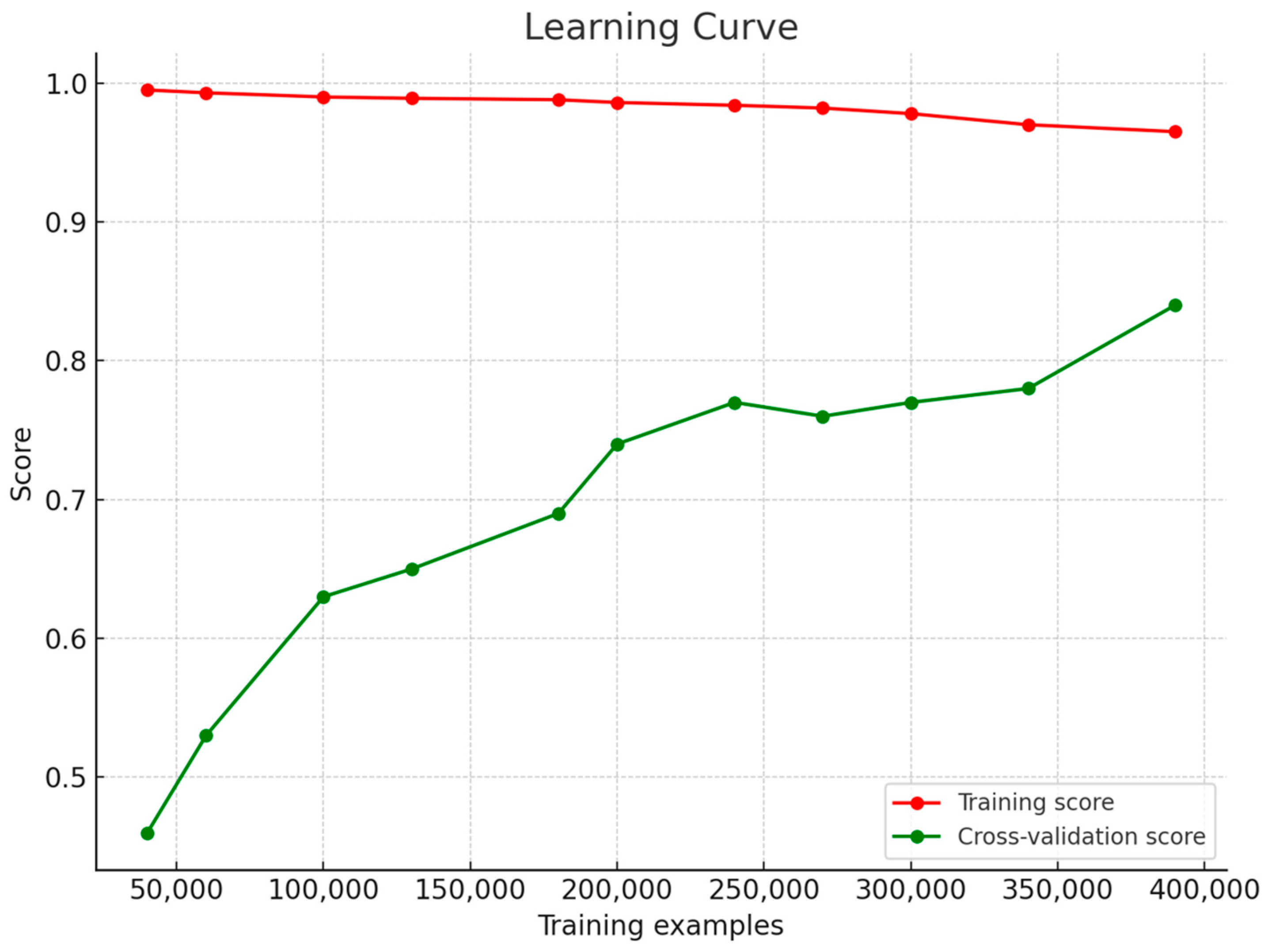
The learning curve graph is an important tool for evaluating the performance of a machine learning model. This graph shows the training and validation accuracy of the model. A training accuracy close to 1.0 suggests that the model may be overfitting the training data, but this is not always the case. To verify overfitting, it is also necessary to examine whether the validation error is high. The learning curve graph of the paper is presented in Figure 11.

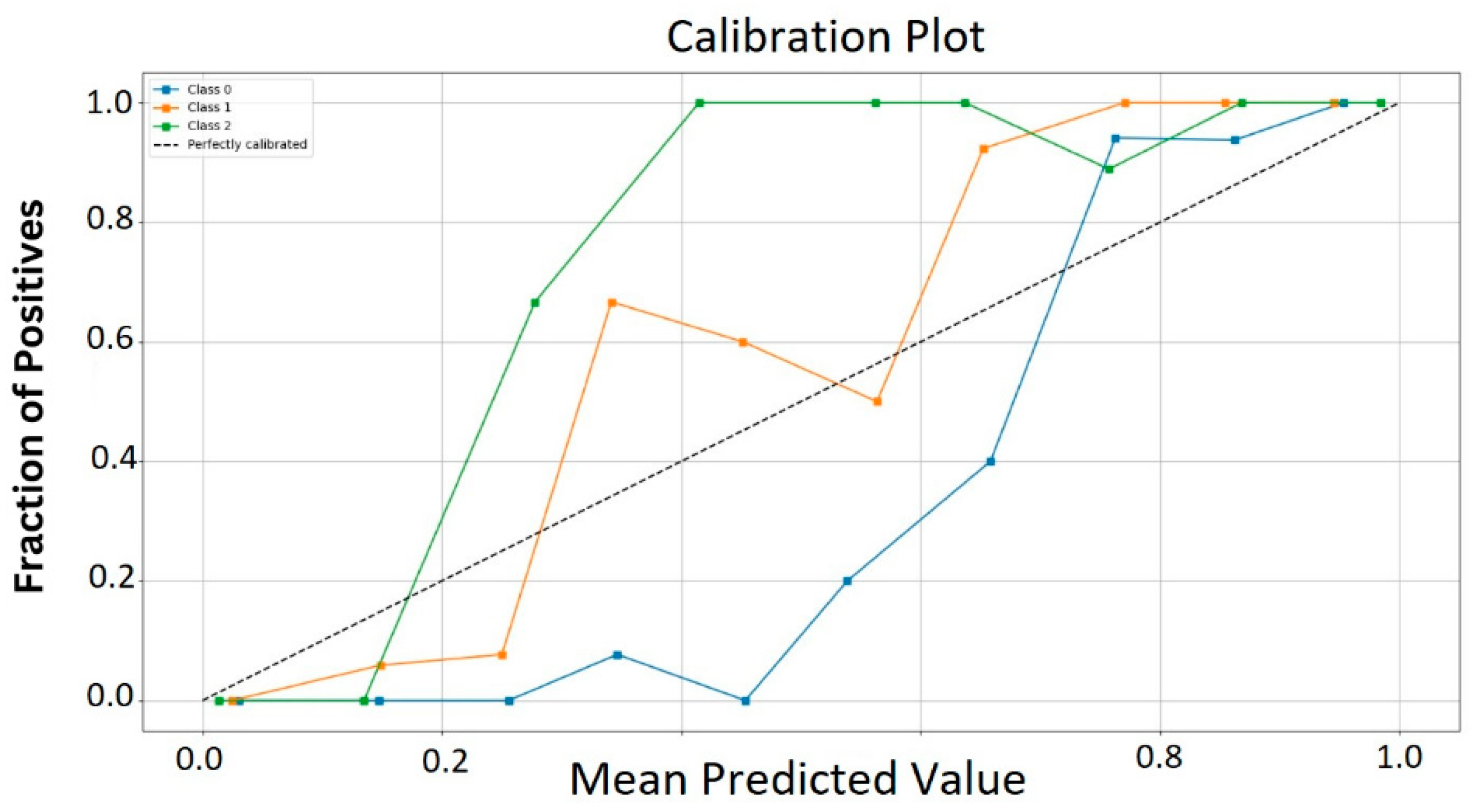
The training error is negligible. The calibration curve helps us understand whether the model is calibrated by comparing the predicted probabilities with the actual results. Ideally, the calibration curve follows the line y = x. An ideal calibration curve shows a linear relationship between predicted probabilities and actual probabilities, and this linear relationship is represented by the dotted line labeled ‘Perfectly Calibrated’. This linear relationship indicates that the predicted probabilities are consistent with the true probabilities. The calibration curve of the paper is shown in Figure 12.

A gain plot shows the cumulative success rate of a model towards a given goal. The gain graph is used to measure the effectiveness and performance of the model in correctly identifying the target audience. The graph visualizes the superiority of the model by comparing the cumulative true positive rate of the model with random selections. The gain graph for the paper is presented in Figure 13.

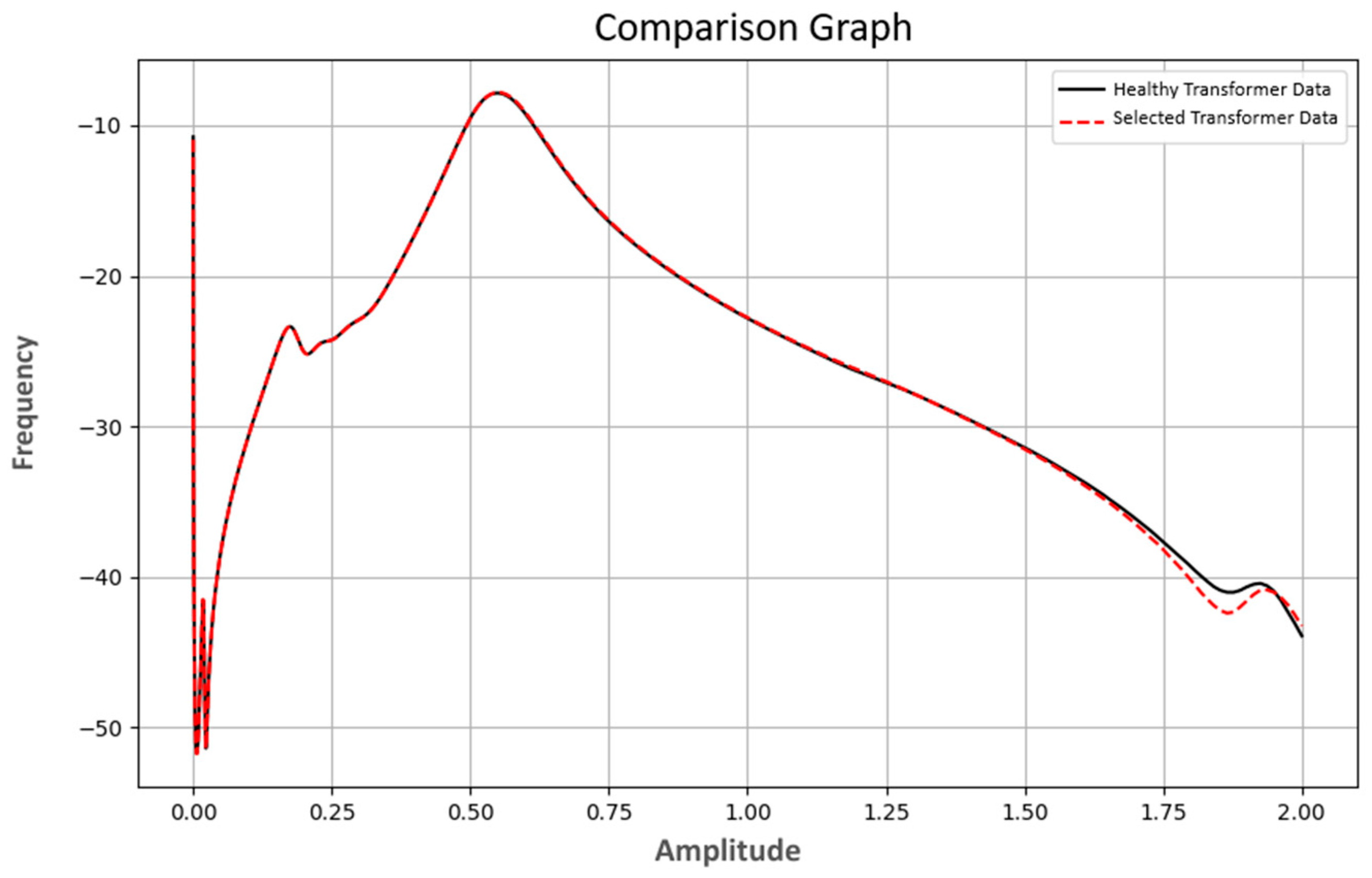
In addition to the performance graphs, the frequency–amplitude plot of a healthy transformer was compared with that of a randomly selected transformer to assess its condition (Figure 14). The graph shows both datasets on the same axes, allowing differences and similarities to be visually analyzed. The black line represents the frequency–amplitude relationship of the healthy transformer, while the red dashed line shows the data of the selected transformer. These comparisons are important for assessing the condition of transformers and detecting faults early. As a result of the analysis, more precise judgments can be made as to whether the selected transformer is healthy or not. In the graph (Figure 14), the frequency–amplitude relationship of a healthy transformer is compared with the frequency–amplitude relationship of a selected transformer for evaluation purposes. According to the analysis of the 1w-1n test data, a total of 1000 data points were examined, with 906 classified as class 0, 41 as class 1, and 53 as class 2. As a result of this classification, the selected transformer was generally assessed to be healthy. Considering the comparison graph and other results, it was concluded that optimal results were achieved.

4.3. General Results and Conclusions

To mathematically evaluate the results of the paper, several performance tests were conducted. In machine learning studies, various performance metrics are used to assess the success of models. In this study, fault detection was performed using transformer data obtained from SFRA tests, and the model’s performance was measured using overall accuracy, precision, recall, MSE, RMSE, and F1 score metrics. These metrics are fundamental indicators for evaluating the accuracy of machine learning models, the rates of false positives and false negatives, as well as the overall balance performance. The performance results obtained from the paper are presented in

Table 4. Performance results of a transformer fault diagnosis model constructed with the GBC algorithm.

Metric	Value
Accuracy	0.9142
Precision	0.9205
Recall	0.9142
F1 Score	0.9141
MSE	0.1143
RMSE	0.1143

. As shown in Table 4, fault detection was performed using transformer data obtained from SFRA tests, and the performance of the model was measured using four metrics: overall accuracy, precision, recall, MSE, RMSE, and F1 score. These metrics are key indicators that evaluate the accuracy, false positive and false negative rates, and overall performance balance of machine learning models. Overall accuracy is a metric frequently used to measure model performance in machine learning and classification problems. A value close to 1 indicates that the model demonstrates high performance. In this study, the accuracy value for the GBC algorithm was calculated to be 0.9142. Overall precision measures the accuracy rate of the model’s positive class predictions.

Precision aims to reduce the rate of false positives. A precision value close to 1 is desirable. In this study, the precision value for the GBC algorithm was determined to be 0.9206. Overall recall is another important metric used to measure model performance in machine learning and classification problems. High recall ensures that the model does not miss real positives. This metric specifically aims to reduce the rate of false negatives. A recall value close to 1 is preferred. In this study, the recall value was found to be 0.9142. The overall F1 score is an important metric used to measure model performance in machine learning and classification problems. The F1 score is the harmonic mean of the precision and recall metrics, allowing the model to evaluate these two metrics in a balanced manner. This metric is particularly useful when there is class imbalance because it considers both the model’s capacity to accurately capture positive examples (recall) and its ability to avoid false positive predictions (precision). The F1 score takes a value between 0 and 1, with a value close to 1 meaning that the model demonstrates both high precision and high recall. In this study, the F1 score was calculated to be 0.9142. Additionally, to evaluate the results of the paper, the mean squared error (MSE) and root mean squared error (RMSE) values were also calculated. The mean squared error (MSE) calculates the average of the squares of the differences between predicted values and actual values. The root mean squared error (RMSE) is obtained by taking the square root of the MSE. Both metrics play a complementary role in assessing the model’s accuracy and prediction performance. The MSE, RMSE, and other performance metric values obtained in this study indicate that the GBC algorithm demonstrates high prediction accuracy and effective performance in transformer fault detection. All these results reveal that the Gradient Boosting Classifier algorithm provides both high accuracy and overall balance for transformer fault detection. The model has exhibited strong performance, particularly in terms of the accuracy of positive predictions and the detection of true positives, proving the reliability and effectiveness of its predictions.

5. Conclusions and Discussion

In this study, we comprehensively addressed the critical role of transformers in electrical power systems and how technological advancements can enhance the efficiency and reliability of these devices. Transformers play a vital role in the processes of electricity generation and distribution. However, to ensure their long lifespan and reliable operation, it is essential to accurately classify and diagnose fault types. This research examined the testing methods developed for the early detection of transformer faults. Innovative modern testing techniques, such as Sweep Frequency Response Analysis (SFRA), have enabled significant advancements by analyzing the frequency response of transformers to detect potential internal damage.

One of the key contributions of this paper to the literature lies in the diagnosis of faulty and healthy transformers through the evaluation of SFRA test results using machine learning techniques and artificial intelligence. An important aspect of this contribution is the creation of three label values related to the condition of the transformer during the assessment. Machine learning algorithms, especially powerful methods like the Gradient Boosting Classifier (GBC), offer substantial contributions to the prediction and prevention of transformer faults. Machine learning technology can make highly accurate fault predictions by learning from large datasets. In this study, the GBC algorithm demonstrated superior performance in three-class classification problems.

Furthermore, this study visually examined the relationship between frequency and amplitude by analyzing performance graphs, clearly highlighting the differences between healthy and faulty transformers. The results obtained from the classification algorithm applied to the dataset, when compared with existing studies in the literature, show that no system currently diagnoses three label values for transformer faults simultaneously using machine learning and artificial intelligence with SFRA data. The applicability of existing studies to fieldwork is also generally limited.

One of the main contributions of this study is that it provides easily interpretable and understandable results. However, like any academic work, this approach is open to further development and enhancement of its usability. Currently, to conduct SFRA and other transformer tests, it is necessary to disconnect the transformer’s power and separate the connections between the feeder and bus bars. In the future, as more research is conducted in this area, SFRA tests could be performed by applying voltages at different frequencies to the transmission lines and bus bars. If the results of these tests can be instantaneously compared using artificial intelligence, it will be possible to conduct real-time tests without cutting power or disconnecting the conductors.

If studies on the classification and processing of SFRA results with machine learning (ML) are expanded to include non-fault-related variations such as humidity, temperature, environmental noise, and test connection discrepancies and are supported by more extensive experimental work, they can play a pioneering role in the design of reliable online SFRA systems in the future. The integrated design of ML-supported online SFRA and Internet of Things (IoT)-based smart transformer monitoring systems will reduce maintenance and production loss costs in transformers and electrical transmission systems and maximize the utilization of existing equipment. The shift from periodic maintenance to condition-based maintenance in power transformers is inevitable. The safe transition to this shift can be achieved through ML-supported systems. Subsequent studies will focus on the design of a reliable online SFRA system.

References

- Chakravorti, S.; Dey, D.; Chatterjee, B. Power Systems. In Recent Trends in the Condition Monitoring of Transformers: Theory, Implementation and Analysis; Springer: London, UK, 2013. [Google Scholar]
- Chandran, L.R.; Babu, G.S.A.; Nair, M.G.; Ilango, K. A review on status monitoring techniques of transformer and a case study on loss of life calculation of distribution transformers. Mater. Today Proc. 2021, 46, 4659–4666. [Google Scholar] [CrossRef]
- Rigatos, G.; Siano, P. Power transformers’ condition monitoring using neural modeling and the local statistical approach to fault diagnosis. Int. J. Electr. Power Energy Syst. 2016, 80, 150–159. [Google Scholar] [CrossRef]
- Jahromi, A.; Piercy, R.; Cress, S.; Fan, W. An approach to power transformer asset management using health index. IEEE Electr. Insul. Mag. 2009, 25, 20–34. [Google Scholar] [CrossRef]
- Khalili Senobari, R.; Sadeh, J.; Borsi, H. Frequency response analysis (FRA) of transformers as a tool for fault detection and location: A review. Electr. Power Syst. Res. 2018, 155, 172–183. [Google Scholar] [CrossRef]
- Gonzalez, C.; Pleite, J.; Valdivia, V.; Sanz, J. An overview of the on line application of frequency response analysis (FRA). In Proceedings of the 2007 IEEE International Symposium on Industrial Electronics, Vigo, Spain, 4–7 June 2007; pp. 1294–1299. [Google Scholar]
- Gomez-Luna, E.; Mayor, G.A.; Gonzalez-Garcia, C.; Guerra, J.P. Current status and future trends in frequency-response analysis with a transformer in service. IEEE Trans. Power Deliv. 2013, 28, 1024–1031. [Google Scholar] [CrossRef]
- Bjelić, M.; Brković, B.; Zarković, M.; Miljković, T. Machine learning for power transformer SFRA based fault detection. Int. J. Electr. Power Energy Syst. 2024, 156, 109779. [Google Scholar] [CrossRef]
- Hashemnia, N.; Abu-Siada, A.; Islam, S. Impact of axial displacement on power transformer FRA signature. In Proceedings of the 2013 IEEE Power & Energy Society General Meeting, Vancouver, BC, Canada, 21–25 July 2013; pp. 1–4. [Google Scholar]
- Paleri, A.; Preetha, P.; Sunitha, K. Frequency Response Analysis (FRA) in power transformers: An approach to locate inter-disk SC fault. In Proceedings of the 2017 IEEE PES Asia-Pacific Power and Energy Engineering Conference (APPEEC), Bangalore, India, 8–10 November 2017; pp. 1–5. [Google Scholar]
- Wang, S.; Yang, F.; Qiu, S.; Zhang, N.; Duan, N.; Wang, S. A New Classification Method for Radial Faults of Transformer Winding by FRA and PSO-RVM. In Proceedings of the 2023 24th International Conference on the Computation of Electromagnetic Fields, Kyoto, Japan, 22–26 May 2023; pp. 1–4. [Google Scholar]
- Kuniewski, M.; Zydron, P. Analysis of the Applicability of Various Excitation Signals for FRA Diagnostics of Transformers. In Proceedings of the 2018 IEEE 2nd International Conference on Dielectrics (ICD), Budapest, Hungary, 1–5 July 2018; pp. 1–4. [Google Scholar]
- Nurmanova, V.; Bagheri, M.; Zollanvari, A.; Aliakhmet, K.; Akhmetov, Y.; Gharehpetian, G.B. A New Transformer FRA Measurement Technique to Reach Smart Interpretation for Inter-Disk Faults. IEEE Trans. Power Deliv. 2019, 34, 1508–1519. [Google Scholar] [CrossRef]
- Wang, S.; Wang, S.; Feng, H.; Guo, Z.; Wang, S.; Li, H. A New Interpretation of FRA Results by Sensitivity Analysis Method of Two FRA Measurement Connection Ways. IEEE Trans. Magn. 2018, 54, 8400204. [Google Scholar] [CrossRef]
- Shintemirov, A. Modelling of power transformer winding faults for interpretation of frequency response analysis (FRA) measurements. In Proceedings of the 4th International Conference on Power Engineering, Energy and Electrical Drives, Istanbul, Türkiye, 13–17 May 2013; pp. 1352–1357. [Google Scholar]
- IEC 60076-1; Power Transformers—Part 1. IEC: General, Geneva, Switzerland, 2011.
- Swift, G.; Molinski, T.S.; Lehn, W. A fundamental approach to transformer thermal modeling—Part I: Theory and equivalent circuit. IEEE Trans. Power Deliv. 2001, 16, 171–175. [Google Scholar] [CrossRef]
- Purnomoadi, A.P.; Fransisco, D. Modeling and diagnostic transformer condition using sweep frequency response analysis. In Proceedings of the 2009 IEEE 9th International Conference on the Properties and Applications of Dielectric Materials, Harbin, China, 19–23 July 2009; IEEE: New York, NY, USA, 2009. [Google Scholar]
- Ludwikowski, K.; Siodla, K.; Ziomek, W. Investigation of transformer model winding deformation using sweep frequency response analysis. IEEE Trans. Dielectr. Electr. Insul. 2012, 19, 1957–1961. [Google Scholar] [CrossRef]
- Omicron FRAnalyzer User Manual, Sweep Frequency Response Analyzer for Power Transformer Winding Diagnosis; Omicron electronics: Kowloon, China, 2009.
- Aamir, K.M.; Sarfraz, L.; Ramzan, M.; Bilal, M.; Shafi, J.; Attique, M. A fuzzy rule-based system for classification of diabetes. Sensors 2021, 21, 8095. [Google Scholar] [CrossRef] [PubMed]
- Cortes, C.; Vapnik, V. Support-vector networks. Mach. Learn. 1995, 20, 273–297. [Google Scholar] [CrossRef]
- Suthaharan, S. Decision Tree Learning. Machine Learning Models and Algorithms for Big Data Classification; Integrated Series in Information Systems; Springer: Boston, MA, USA, 2016; pp. 237–269. [Google Scholar]
- Breiman, L. Random forests. Mach. Learn. 2001, 45, 5–32. [Google Scholar] [CrossRef]