A Permanent-Magnet Eddy-Current Loss Analytical Model for Axial Flux Permanent-Magnet Electric Machine Accounting for Stator Saturation

Abstract

This paper introduces a hybrid analytical model (HAM) for the evaluation of permanent-magnet (PM) eddy-current loss in dual-stator single-rotor axial flux permanent-magnet machine (AFPMM), accounting for stator saturation. The proposed model integrates the magnetic equivalent circuit (MEC) with an analytical model based on scalar magnetic potential, enabling simultaneous consideration of different rotor positions and stator slotting effects. The three-dimensional finite element method (3D-FEM) validates the no-load and armature reaction magnetic field calculated by HAM, as well as the PM eddy-current loss under both no-load and load conditions. Compared to 3D-FEM, the proposed model reduces the calculation time by more than 98% with an error of no more than 18%, demonstrating a significant advantage in terms of computational time. Based on the proposed model, the effects of air-gap length and slot opening width on PM eddy-current loss are analyzed; the results indicate that reducing the slot opening width can effectively mitigate PM eddy-current loss for AFPMM.

1. Introduction

The dual-stator single-rotor AFPMM holds significant potential for application in electric vehicles, flywheel energy storage systems, and aerospace due to its compact structure and high torque density [1,2,3,4,5]. As power density requirements increase in these applications, the compact design of AFPMM poses challenges to the rotor heat dissipation, particularly when fractional slot centralized windings are employed, leading not only to excessive temperature rise in the PM but also potentially causing irreversible demagnetization under severe conditions [6,7,8]. However, existing methods for calculating PM eddy-current losses in AFPMM predominantly rely on 3D-FEM, which is very time-consuming. Consequently, fast and accurate evaluation of the PM eddy-current loss is essential for AFPMM.

Currently, numerous studies have proposed analytical methods to evaluate PM eddy-current loss in radial flux machines. In [9,10], the subdomain method was used to calculate PM eddy-current loss under no-load and loaded conditions, respectively. In [11], the subdomain method was further extended by deriving the PM eddy-current loss caused by each harmonic of the armature reaction field. In [12], an analytical model based on image theory that accounts for the three-dimensional distribution of PM eddy currents was introduced. However, all of the studies mentioned above overlook the influence of eddy-current reaction field and stator saturation.

In radial flux machines, the 2D analytical model assumes that the length of the PM is significantly larger than its width, so the eddy-current loss in the circumferential direction is neglected. However, for AFPMMs, the radial length of the PM is comparable to its circumferential length, making the eddy currents in the circumferential direction non-negligible. Consequently, the conventional 2D method is not fully applicable to AFPMMs. To address this issue, a multilayer-2D coupled model for YASA machine is proposed in [13], effectively transforming the 3D finite element model into a multilayer-2D finite element model. The total PM loss is obtained by summing the eddy-current losses in each layer, which significantly reduces computation time. However, this method requires substantial post-processing work. Studies [14,15] combined the conformal transformation method with the resistive network model, and the reaction field of eddy current was represented by inductance, thereby establishing an analytical model for PM eddy-current losses in yokeless and segmented armature (YASA) AFPMM. Similarly, [16] simplified the 3D eddy-current path for a dual-stator, single-rotor AFPMM and calculated the PM eddy-current loss. Nevertheless, these studies neglected the effect of stator saturation on PM eddy-current loss.

This paper integrates a HAM with a PM resistance network model to accurately calculate the PM eddy-current losses in AFPMM. To account for stator saturation, the hybrid model adopts an MEC model for the stator in order to consider the effect of stator saturation. Meanwhile, an analytical model based on scalar magnetic potential is utilized in the air-gap and PM regions. By combining these two models, the magnetic field distribution in the AFPMM is obtained. A resistance network model of the PM is then established, which allows for analytical calculation of PM eddy-current loss under both no-load and load conditions. The accuracy of the proposed HAM is validated using 3D-FEM. Finally, the effects of slot opening width and air-gap length on the PM eddy-current loss in AFPMM are analyzed through the proposed HAM.

2. Hybrid Analytical Model

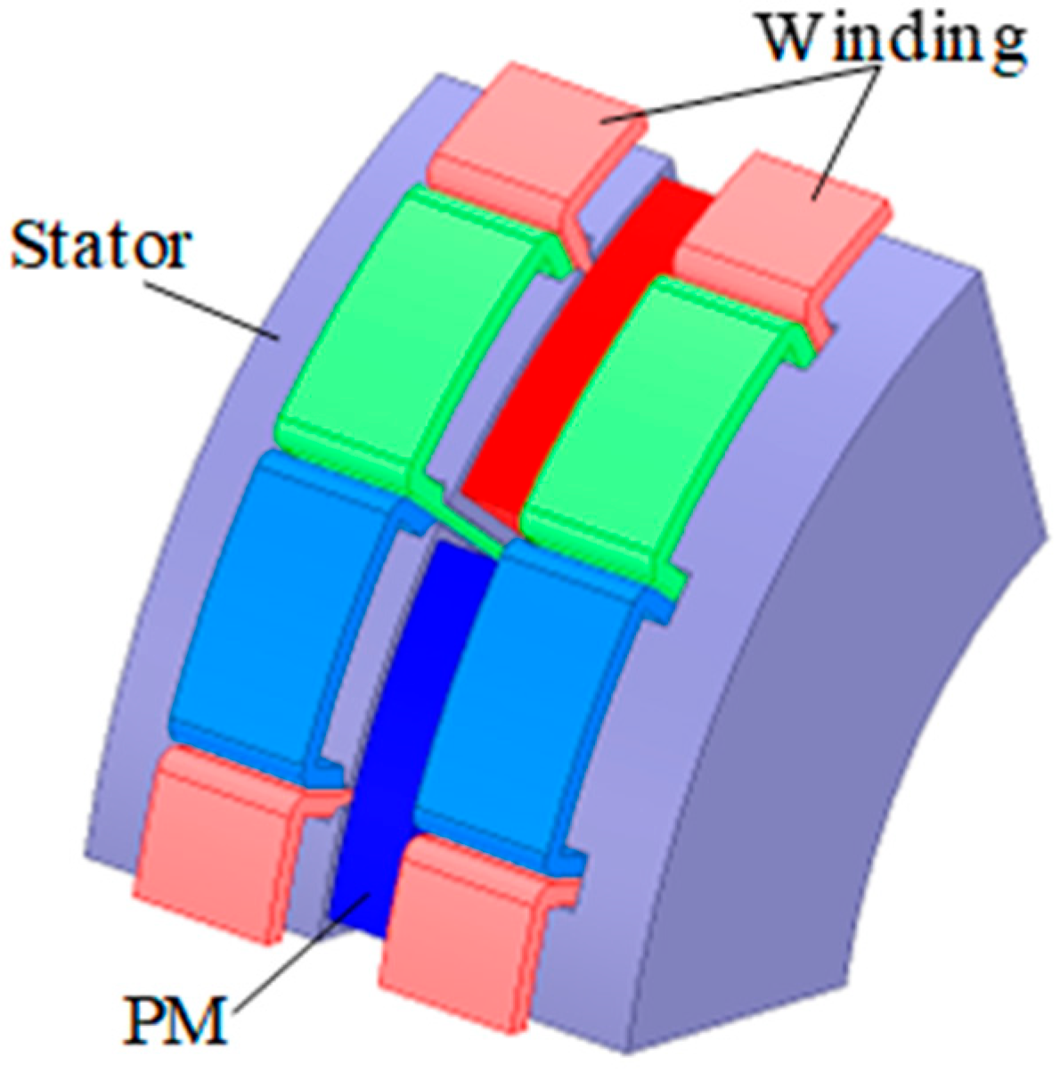
The saturation of the stator core is considered by using the MEC model. For the conventional magnetic network model, the air-gap region and the PM region in MEC needs to be reconstructed as the rotor position changes. To avoid this problem, these two regions are modeled by the analytical model. In this paper, an eighteen-slot, twelve-pole, dual-stator, single-rotor AFPMM is used as an example. Due to the symmetry and periodicity of the magnetic flux path, the one/sixth model of the machine with one stator is modeled, as shown in Figure 1.

Since the magnetic field of the AFPMM is distributed in three dimensions, the quasi-3D method is used to convert the 3D-AFPMM into a combination of n_s 2D linear machines without end effects. The thickness of each 2D linear machine is l_s, which can be calculated as follows:

$$l_s={\displaystyle \frac{R_{\mathrm{o}}-R_{\mathrm{i}}}{n_s}}$$

(1)

where n_s is the number of the 2D linear machine, and R_o and R_i are the outer and inner radius of the stator.

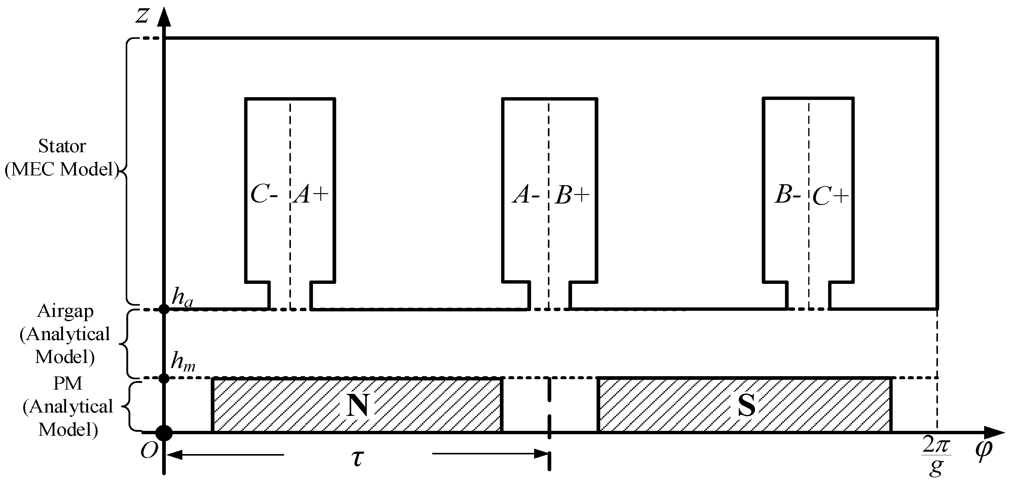
Due to the periodicity and symmetry of the magnetic flux in dual-stator single-rotor AFPMM, to avoid unnecessary computations, it is adequate to model only half of the 1/6 model of the AFPMM. The equivalent model for a 2D linear machine is shown in Figure 2, where h_m is the thickness of PM, τ is the pole pitch, and g is the greatest common divisor of the number of slots and poles (In this case, g = 6 since the pole number and slot number are 12 and 18, respectively). To simplify the solving process of HAM, the following assumptions are made:

(1)

The permeability of the PM is same as vacuum, and the relative permeability for PM is taken as 1;

(2)

The leakage magnetic flux at the inner and outer diameter is neglected.

The magnetic field for an electric machine is considered as a quasi-static field, and therefore, the magnetic field strength H can be expressed as follows:

$$H=-\nabla U$$

(2)

where U is the scalar magnetic potential.

For magnetic materials such as PM, the magnetic density can be stated as follows:

$$B={\mu }_0{\mu }_{r}H+{\mu }_{0}M$$

(3)

For non-magnetic materials such as air, the magnetic density can be given by the following:

$$B={\mu }_0{\mu }_{r}H$$

(4)

where μ₀ is the permeability of vacuum, μ_r is the relative permeability of the medium, and M is the magnet magnetization vector. From Equations (2)–(4), it can be known that as long as the scalar magnetic potential equation within the corresponding region is obtained, the magnetic flux density distribution can be calculated.

2.1. General Scalar Magnetic Potential Solution of Analytical Model

2.1.1. PM Region

The Laplace equation for the scalar magnetic potential in the PM region can be expressed as follows:

$${\displaystyle \frac{1}{r^2}}{\displaystyle \frac{{\partial }^2{U}_{\mathrm{I}}}{\partial {\phi }^2}}+{\displaystyle \frac{{\partial }^2{U}_{\mathrm{I}}}{\partial z^2}}=0$$

(5)

where U_I is the scalar magnetic potential in PM region, and r stands for radius. The internal boundary conditions can be denoted as follows:

$$\left\{\begin{array}{l}{\left.{\displaystyle \frac{\partial U_{\mathrm{I}}}{\partial \phi }}\right|}_{z=0}=0\\ {\left.{\displaystyle \frac{\partial U_{\mathrm{I}}}{\partial \phi }}\right|}_{\phi =0}={\left.{\displaystyle \frac{\partial U_{\mathrm{I}}}{\partial \phi }}\right|}_{\phi ={\displaystyle \frac{2\pi }{g}}}\\ 0<z\le h_m\\ 0\le \phi \le {\displaystyle \frac{2\pi }{g}}\end{array}\right.$$

(6)

By means of the separated variable method, the general solution of U_I can be expressed as follows:

$$U_{\mathrm{I}}={\displaystyle \sum _{n=1}^{\infty }\left[A_1\sinh \left(\frac{ng}{r}z\right)\cdot \sin (ng\phi )+B_1\sinh \left(\frac{ng}{r}z\right)\cdot \cos (ng\phi )\right]}$$

(7)

where n is the harmonics number considered in the PM region, and A₁ and B₁ are the undetermined constants.

Based on the principle of the electromagnetic field, the circumferential and axial magnetic field components H_I,φ and H_I,z can be expressed as the negative gradient of the scalar magnetic potential U_I:

$$H_{\mathrm{I},\phi }=-{\displaystyle \frac{1}{r}}{\displaystyle \frac{\partial U_{\mathrm{I}}}{\partial \phi }},H_{\mathrm{I},z}=-{\displaystyle \frac{\partial U_{\mathrm{I}}}{\partial z}}$$

(8)

According to Equation (8), the circumferential and axial magnetic flux density of the PM region can be expressed as

$$\begin{array}{cc}{B}_{\mathrm{I},\phi }& ={\mu }_0{H}_{\mathrm{I},\phi }\\ & =-{\mu }_0{\displaystyle \frac{ng}{r}}{\displaystyle \sum _{n=1}^{\infty }\left[\begin{array}{l}{A}_1\sinh \left(\frac{ng}{r}z\right)\cdot \cos (ng\phi )-\\ A_2\sinh \left(\frac{ng}{r}z\right)\cdot \sin (ng\phi )\end{array}\right]}\end{array}$$

(9)

$$\begin{array}{cc}{B}_{\mathrm{I},z}& ={\mu }_0\left(H_{\mathrm{I},z}+M_z\right)\\ & =-{\mu }_0{\displaystyle \frac{ng}{r}}{\displaystyle \sum _{n=1}^{\infty }\left[\begin{array}{l}{A}_1\left(\cosh \left(\frac{ng}{r}z\right)-\frac{r}{ng}{M}_{cn}\right)\cdot \sin (ng\phi )+\\ A_2\left(\cosh \left(\frac{ng}{r}z\right)-\frac{r}{ng}{M}_{sn}\right)\cdot \cos (ng\phi )\end{array}\right]}\end{array}$$

(10)

where M_z is the magnetization vector in the axial direction. M_z, M_cn, and M_sn are given by the following:

$$\left\{\begin{array}{l}{M}_z={\displaystyle \sum _n^{\infty }\left(M_{cn}\sin (ng\phi )+M_{sn}\cos (ng\phi )\right)}\\ M_{cn}=M_{zk}\cos \left(ng({\omega }_{\mathrm{r}}t+{\phi }_0)\right)\\ M_{sn}=M_{zk}\sin \left(ng({\omega }_{r}t+{\phi }_0)\right)\\ M_{zk}={\displaystyle \frac{4B_{\mathrm{r}}}{ng\tau {\mu }_0}}\sin ({\displaystyle \frac{ng\tau {\alpha }_p}{2}})\sin {\displaystyle \frac{ng\tau }{2}}\end{array}\right.$$

(11)

where B_r is the remanence of PM, ω_r is the rotor rotational speed, φ₀ is the rotor initial position, and α_p is the pole arc coefficient.

2.1.2. Air-Gap Region

In air-gap region, the Laplace’s equation is as follows:

$${\displaystyle \frac{1}{r^2}}{\displaystyle \frac{{\partial }^2{U}_{\mathrm{II}}}{\partial {\phi }^2}}+{\displaystyle \frac{{\partial }^2{U}_{\mathrm{II}}}{\partial z^2}}=0$$

(12)

where U_II is the scalar magnetic potential in air-gap region. The internal boundary conditions are satisfied as follows:

$$\left\{\begin{array}{l}{\left.{\displaystyle \frac{\partial U_{\mathrm{I}\mathrm{I}}}{\partial \phi }}\right|}_{\phi =0}={\left.{\displaystyle \frac{\partial U_{\mathrm{I}\mathrm{I}}}{\partial \phi }}\right|}_{\phi ={\displaystyle \frac{2\pi }{g}}}\\ h_m<z\le h_a\\ 0\le \phi \le {\displaystyle \frac{2\pi }{g}}\end{array}\right.$$

(13)

The general solution of U_II is as follows:

$$U_{\mathrm{II}}={\displaystyle \sum _{n=1}^{\infty }\left[\begin{array}{l}\left(A_2\sinh \left(\frac{ng}{r}z\right)+B_2\cosh \left(\frac{ng}{r}z\right)\right)\cdot \sin (ng\phi )+\\ \left(C_2\sinh \left(\frac{ng}{r}z\right)+D_2\cosh \left(\frac{ng}{r}z\right)\right)\cdot \cos (ng\phi )\end{array}\right]}$$

(14)

where A₂, B₂, C₂, and D₂ are the undetermined constants.

At the interface (z = h_m) between the air-gap region and the PM region, since the permeability of the two regions are the same, according to the boundary conditions of the electromagnetic field, the circumferential and axial magnetic field strengths are equal at the boundary z = h_m. The boundary conditions can be denoted as follows:

$$\left\{\begin{array}{l}{\left.{\displaystyle \frac{\partial U_{\mathrm{I}}}{\partial \phi }}\right|}_{z=h_m}={\left.{\displaystyle \frac{\partial U_{\mathrm{II}}}{\partial \phi }}\right|}_{z=h_m}\\ {\left.{\displaystyle \frac{\partial U_{\mathrm{I}}}{\partial z}}\right|}_{z=h_m}={\left.{\displaystyle \frac{\partial U_{\mathrm{II}}}{\partial z}}\right|}_{z=h_m}\end{array}\right.$$

(15)

Substituting Equation (15) into Equations (14) and (7), the undetermined constants in U_II can be represented as follows:

$$\left\{\begin{array}{l}{A}_2=A_1-{\displaystyle \frac{r}{ng}}{M}_{cn}\cosh \left({\displaystyle \frac{ng}{r}}{h}_m\right)\\ B_2={\displaystyle \frac{r}{ng}}{M}_{cn}\sinh \left({\displaystyle \frac{ng}{r}}{h}_m\right)\\ C_2=B_1-{\displaystyle \frac{r}{ng}}{M}_{sn}\cosh \left({\displaystyle \frac{ng}{r}}{h}_m\right)\\ D_2={\displaystyle \frac{r}{ng}}{M}_{sn}\sinh \left({\displaystyle \frac{ng}{r}}{h}_m\right)\end{array}\right.$$

(16)

Thus, the scalar magnetic potential U_II can be rewritten as

$$\begin{array}{c}{U}_{\mathrm{II}}={\displaystyle \sum _{n=1}^{\infty }\left[\left(\begin{array}{l}\left(A_1-\frac{r}{ng}{M}_{cn}\cosh \left(\frac{ng}{r}{h}_m\right)\right)\sinh \left(\frac{ng}{r}z\right)+\\ \frac{r}{ng}{M}_{cn}\sinh \left(\frac{ng}{r}{h}_m\right)\cosh \left(\frac{ng}{r}z\right)\end{array}\right)\cdot \sin (ng\phi )\right]+}\\ {\displaystyle \sum _{n=1}^{\infty }\left[\left(\begin{array}{l}\left(B_1-\frac{r}{ng}{M}_{sn}\cosh \left(\frac{ng}{r}{h}_m\right)\right)\sinh \left(\frac{ng}{r}z\right)+\\ \frac{r}{ng}{M}_{sn}\sinh \left(\frac{ng}{r}{h}_m\right)\cosh \left(\frac{ng}{r}z\right)\end{array}\right)\cdot \cos (ng\phi )\right]}\end{array}$$

(17)

The circumferential and axial component of magnetic flux density in the air gap can be given by the following:

$$\begin{array}{c}{B}_{\mathrm{II},\phi }=-{\mu }_0{\displaystyle \frac{ng}{r}}{\displaystyle \sum _{n=1}^{\infty }\left[\left(\begin{array}{l}\left(A_1-\frac{r}{ng}{M}_{cn}\cosh \left(\frac{ng}{r}{h}_m\right)\right)\sinh \left(\frac{ng}{r}z\right)+\\ \frac{r}{ng}{M}_{cn}\sinh \left(\frac{ng}{r}{h}_m\right)\cosh \left(\frac{ng}{r}z\right)\end{array}\right)\cdot \cos (ng\phi )\right]+}\\ {\mu }_0{\displaystyle \frac{ng}{r}}{\displaystyle \sum _{n=1}^{\infty }\left[\left(\begin{array}{l}\left(B_1-\frac{r}{ng}{M}_{sn}\cosh \left(\frac{ng}{r}{h}_m\right)\right)\sinh \left(\frac{ng}{r}z\right)+\\ \frac{r}{ng}{M}_{sn}\sinh \left(\frac{ng}{r}{h}_m\right)\cosh \left(\frac{ng}{r}z\right)\end{array}\right)\cdot \sin (ng\phi )\right]}\end{array}$$

(18)

$$\begin{array}{c}{B}_{\mathrm{II},z}=-{\mu }_0{\displaystyle \frac{ng}{r}}{\displaystyle \sum _{n=1}^{\infty }\left[\left(\begin{array}{l}\left(A_1-\frac{r}{ng}{M}_{cn}\cosh \left(\frac{ng}{r}{h}_m\right)\right)\cos h\left(\frac{ng}{r}z\right)+\\ \frac{r}{ng}{M}_{cn}\sinh \left(\frac{ng}{r}{h}_m\right)\sinh \left(\frac{ng}{r}z\right)\end{array}\right)\cdot \sin (ng\phi )\right]-}\\ {\mu }_0{\displaystyle \frac{ng}{r}}{\displaystyle \sum _{n=1}^{\infty }\left[\left(\begin{array}{l}\left(B_1-\frac{r}{ng}{M}_{sn}\cosh \left(\frac{ng}{r}{h}_m\right)\right)\cosh \left(\frac{ng}{r}z\right)+\\ \frac{r}{ng}{M}_{sn}\sinh \left(\frac{ng}{r}{h}_m\right)\sinh \left(\frac{ng}{r}z\right)\end{array}\right)\cdot \cos (ng\phi )\right]}\end{array}$$

(19)

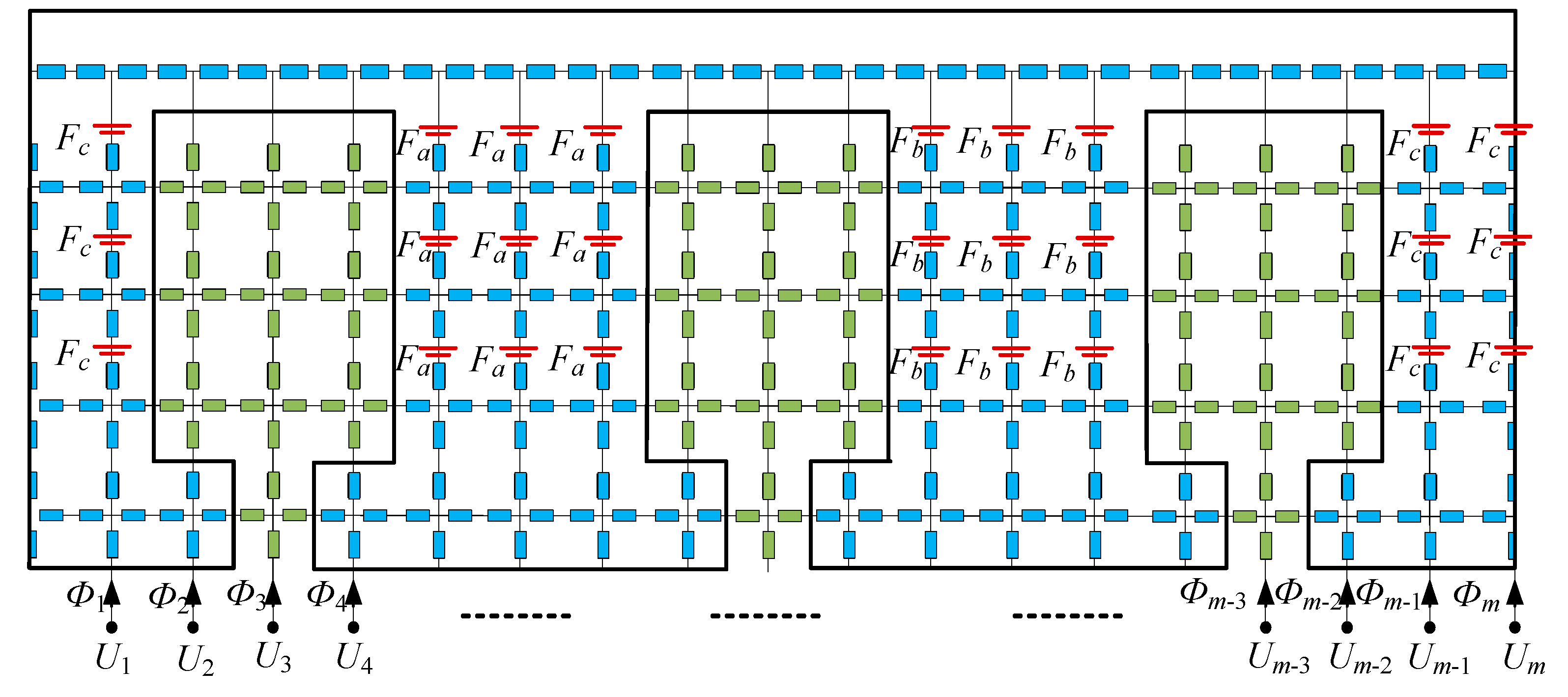
2.2. Stator MEC Model

The stator MEC model is shown in Figure 3. Along the axial direction, the stator is divided into m columns, which means that the surface of stator (interface between air-gap region and stator) has a total of m magnetic potential nodes, represented as U₁, U₂, …, U_m. The magnetic flux that flows into each node of the stator surface is denoted by Φ₁, Φ₂, …, Φ_m, and the magnetic potential of armature winding is given by F_a, F_b, and F_c.

According to Kirchhoff’s voltage law, the magnetic potential of each node (U_node) and the flux of each branch (Φ_branch) in the MEC model can be obtained by the node voltage method:

$$\left\{\begin{array}{l}{U}_{\mathrm{node}}={\displaystyle \frac{-AG{U}_s}{AG{A}^T}}\\ {\varphi }_{\mathrm{branch}}=G{A}^T{U}_{\mathrm{node}}\end{array}\right.$$

(20)

where U_s is the matrix of magnetic potential sources combined with F_a, F_b, F_c, and U₁, U₂, …, U_m, A is the relation matrix of MEC model, and G is the permeance matrix. More details about the construction of the MEC model and the solution process can be found in the studies [17,18].

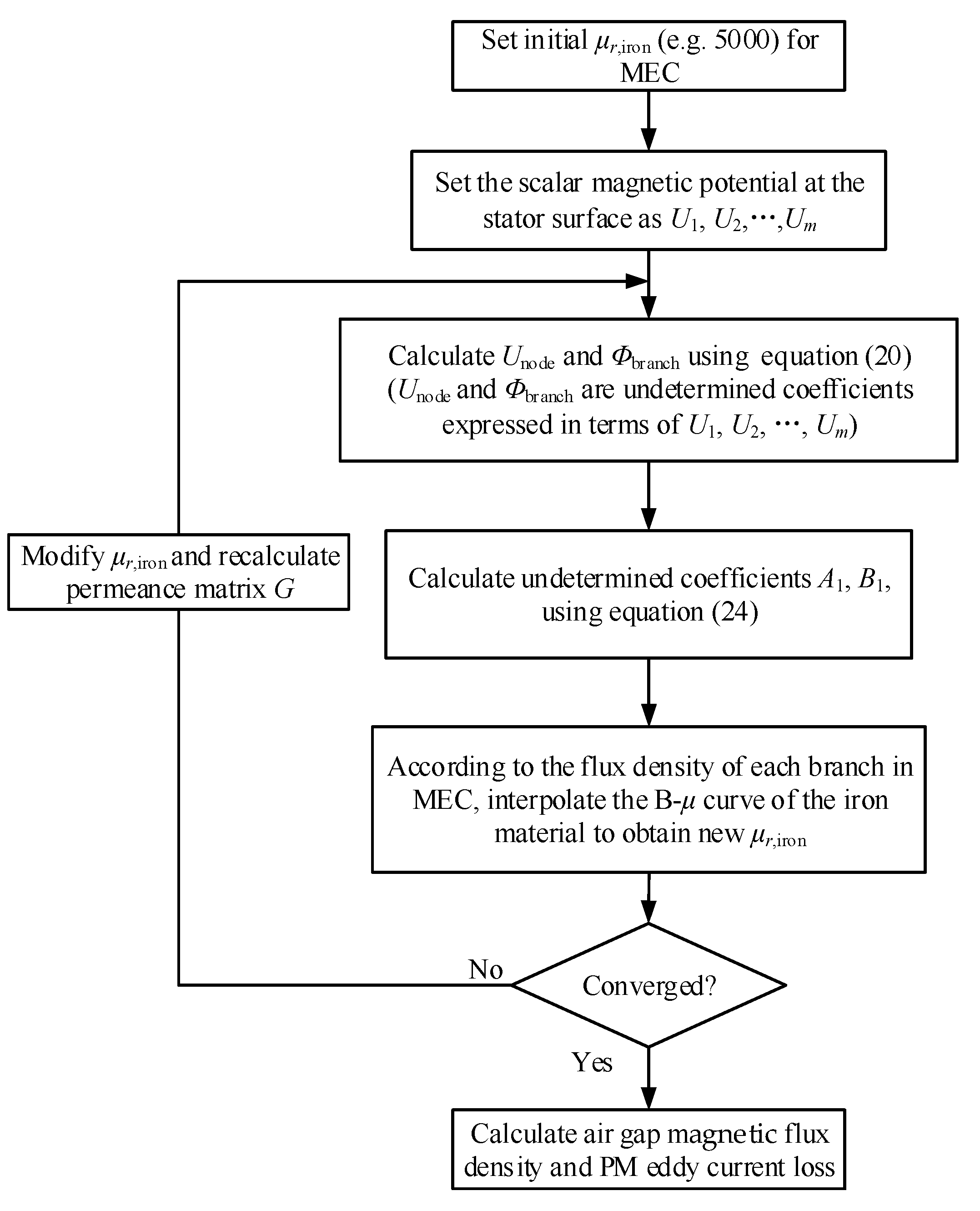
2.3. Solving Process of Hybrid Analytical Model

Because the stator MEC model is divided into m columns, the scalar magnetic potential of each node at the stator surface U₁, U₂, …, U_m can be given by the following:

$$U_{MEC}\left(\phi \right)=\left\{\begin{array}{l}{U}_1,0\le \phi \le {\displaystyle \frac{2\pi }{\mathrm{g}\cdot m}}\\ U_2,{\displaystyle \frac{2\pi }{\mathrm{g}\cdot m}}\le \phi \le 2\cdot {\displaystyle \frac{2\pi }{\mathrm{g}\cdot m}}\\ ⋮\\ U_m,\left(m-1\right){\displaystyle \frac{2\pi }{\mathrm{g}\cdot m}}\le \phi \le m\cdot {\displaystyle \frac{2\pi }{\mathrm{g}\cdot m}}\end{array}\right.$$

(21)

To facilitate the association of the magnetic scalar potential at the stator surface in the MEC model with air-gap scalar magnetic potential U_II, U_MEC(φ) can be rewritten in Fourier series form:

$$U_{MEC}\left(\phi \right)={\displaystyle \frac{a_0}{2}}+{\displaystyle \sum _{n=1}^{\infty }\left[a_n\cos \left(ng\phi \right)+b_n\cos \left(ng\phi \right)\right]}$$

(22)

where a₀, a_n, and b_n are given by

$$\left\{\begin{array}{l}{a}_0={\displaystyle \frac{2}{m}}{\displaystyle \sum _{k=1}^m{U}_k}\\ a_n={\displaystyle \frac{2}{n\pi }}\sin \left({\displaystyle \frac{n\pi }{m}}\right){\displaystyle \sum _{k=1}^m\left[U_k\cos \left(\frac{\left(2k-1\right)\cdot n\pi }{m}\right)\right]}\\ b_n={\displaystyle \frac{2}{n\pi }}\sin \left({\displaystyle \frac{n\pi }{m}}\right){\displaystyle \sum _{k=1}^m\left[U_k\sin \left(\frac{\left(2k-1\right)\cdot n\pi }{m}\right)\right]}\end{array}\right.$$

(23)

In accordance with the continuity boundary condition of the electromagnetic field, the magnetic scalar potentials of the MEC model and analytical model at the interface (z = h_a) are equal, and the magnetic flux that flows into the MEC model is exactly equal to the magnetic flux that flows out of the analytical model, which can be denoted as follows:

$$\left\{\begin{array}{l}{\left.U_{MEC}\right|}_{z=h_a}={\left.U_{\mathrm{II}}\right|}_{z=h_a}\\ {\varphi }_k={\mu }_0{l}_s{\displaystyle {\int }_{\left(k-1\right)\frac{2\pi }{g\cdot m}}^{k\frac{2\pi }{g\cdot m}}{\left.B_{\mathrm{I}\mathrm{I},z}\right|}_{z=h_a}d\phi ,1\le }k\le m\end{array}\right.$$

(24)

where Φ_k is the magnetic flux flowing into the kth nodes (U_k) at the stator surface. It is obtained by Equation (20). Solving the above equation, the undetermined constants A₁ and B₁ can be determined, and so can the circumferential and axial component of magnetic flux density in both the air-gap region and PM region. It should be noted that in order to take into account the saturation effect of the iron core, the permeance of each branch in MEC needs to be calculated by an iteration process searching the B-μ curve of iron material. The calculation flowchart is shown in Figure 4.

3. Resistance Equivalent Network Model of PM

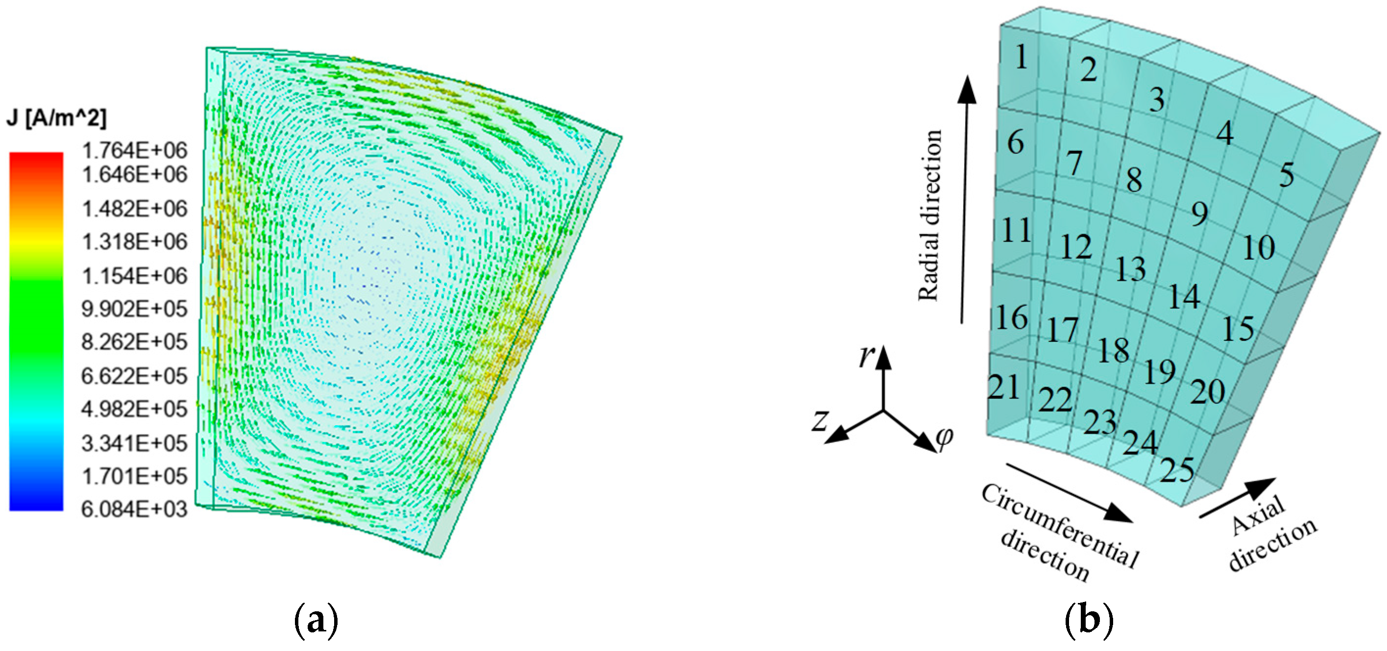
In the 2D PM loss analytical model in conventional radial flux motors, the axial length is assumed to be much larger than the circumferential length, such that only eddy currents along the axial direction within the PM are considered. However, for AFPMM, the circumferential length of the permanent magnet is comparable to its radial length. Consequently, the eddy current within the PM includes both circumferential and radial components, which are indispensable, as shown in Figure 5a. To account for this effect, the PM is divided into segments along both the radial and circumferential directions to form a resistance network, as shown in Figure 5b. 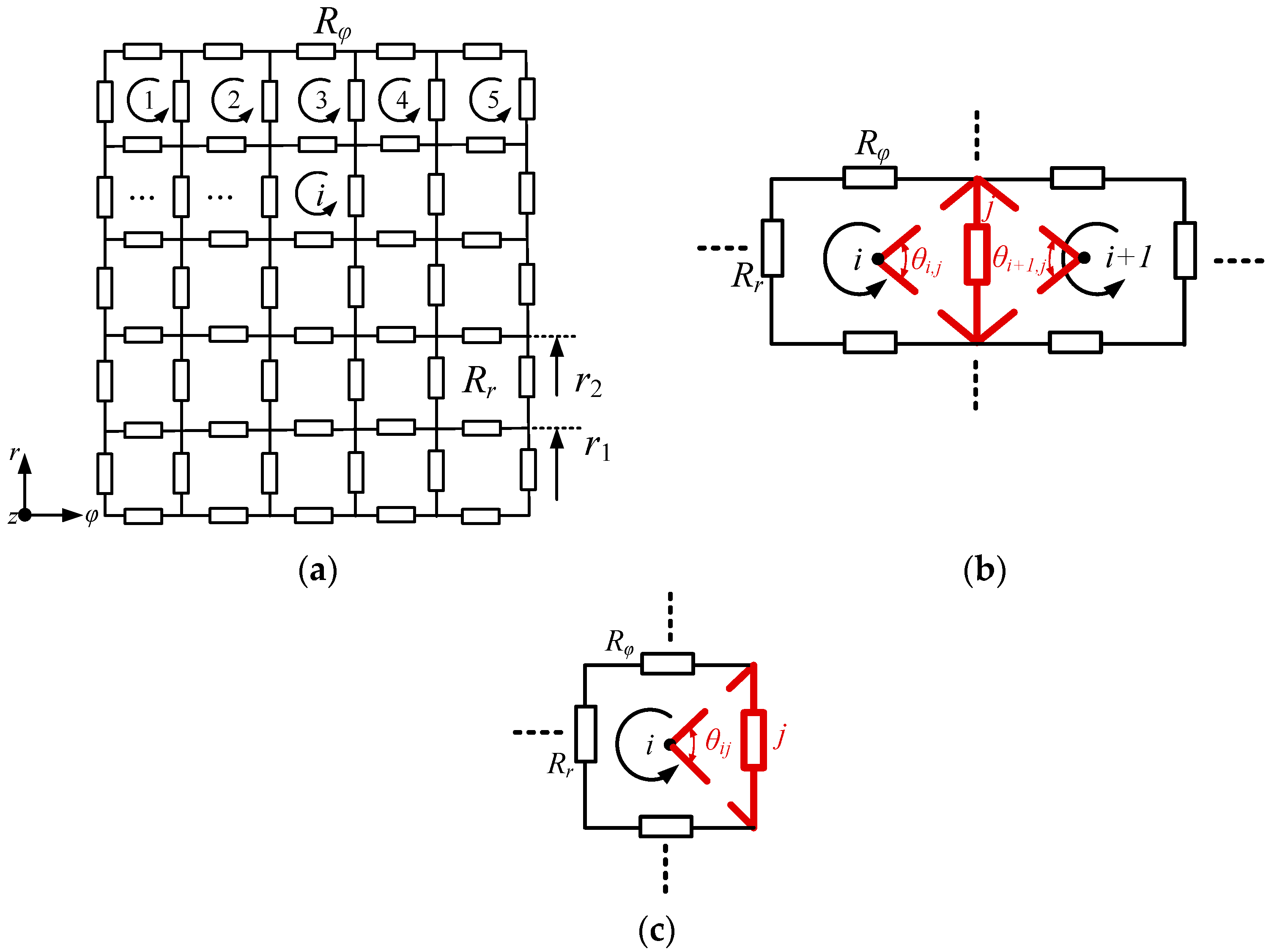These segments are equivalent to interconnected resistance; thus, a resistance network consisting of multiple resistance branches, as shown in Figure 6, is constructed. The voltage source in the circuit is the induced voltage caused by the stator slotting and armature winding harmonics; by solving the resistance loss of each branch in the resistance network, the eddy-current loss of the whole piece of the PM can be obtained.

In Figure 6a, R_r and R_φ are equivalent resistances in the radial and circumferential directions, respectively:

$$\left\{\begin{array}{l}{R}_r={\displaystyle \frac{1}{{\sigma }_{\mathrm{pm}}}}{\displaystyle {\int }_{r_1}^{r_2}\frac{p{\alpha }_p{N}_{\phi }dr}{\mathsf{\pi }r{h}_m}}\\ R_{\phi }={\displaystyle \frac{\mathsf{\pi }\left(r_2+r_1\right)N_r}{2{\sigma }_{\mathrm{pm}}p{\alpha }_p\left[h_m\cdot \left(r_2-r_1\right)\right]}}\end{array}\right.$$

(25)

where σ_pm is the conductivity of PM, and N_r and N_φ are both 5 and represent the number of layers divided in radial and circumferential directions, respectively.

The induced voltage E_i,n induced by nth magnetic flux harmonic in ith resistance sub-circuit can be expressed as follows:

$$\left\{\begin{array}{l}{E}_{i,n}=-{\displaystyle \frac{d{\Phi }_{\mathrm{pm},in}}{dt}}\\ {\Phi }_{\mathrm{pm},in}={\displaystyle \int B_{z,n}d{S}_i={\displaystyle \iint B_{z,n}rdrd\phi }}\end{array}\right.$$

(26)

where Φ_pm,in is the nth magnetic flux harmonic in ith sub-circuit, B_z,_n represents the nth axial flux density harmonic on the surface of PM, and S_i is the area of ith sub-circuit.

The induced voltage E_b,_j in branch j can be divided into two cases. One is when branch j is located between two sub-circuits, in which case E_b,_j is contributed by both sub- circuits, as shown in Figure 6b. The other case is when branch j is at the edge of the resistance network, in which case E_b,_j is only related to one sub-circuit, as shown in Figure 6c. The E_b,_j can be denoted as follows [15]:

$$\left\{\begin{array}{ll}{E}_{\mathrm{b},j}={\displaystyle \frac{1}{2\mathsf{\pi }}}\left({\theta }_{i,j}{\displaystyle \sum _n{E}_{i,n}}+{\theta }_{i+1,j}{\displaystyle \sum _n{E}_{i+1,n}}\right)& \mathrm{case}1\\ E_{\mathrm{b},j}={\displaystyle \frac{1}{2\mathsf{\pi }}}{\theta }_{i,j}{\displaystyle \sum _n{E}_{i,n}}& \mathrm{case}2\end{array}\right.$$

(27)

where θ_i,j is the angle between the center of ith resistance sub-circuit and branch j.

Since the induced voltage and resistance for branch j is determined, the current in branch j is also determined:

$$I_{\mathrm{b},j}={\displaystyle \frac{E_{\mathrm{b},j}}{R_j}}$$

(28)

where R_j is the resistance for branch j.

After the induced voltage E_b,j and current I_b,j for branch j are both derived, the eddy-current loss in PM can be calculated according to Joule’s Law:

$$P_{\mathrm{eddy}}={\displaystyle \sum _j{E}_{\mathrm{b},j}\cdot I_{\mathrm{b},j}}$$

(29)

4. Finite Element Validation

To verify the correctness of the HAM, the magnetic field distribution and permanent-magnet eddy-current loss of an AFPMM are calculated by the finite element method (FEM). The basic parameters of the AFPMM are shown in

Table 1. Basic parameters of the AFPMM.

Parameter	Value	Unit	Parameter	Value	Unit
Outer radius	130	mm	Rated power	20	kW
Inner radius	75	mm	Rated current	80	A
Axial length of stator	45	mm	Rated speed	1200	r/min
Air-gap length	1.2	mm	Slots and Poles	18S12P	-
Slot opening	3	mm	Conductors per slot	26	-
PM thickness	12	mm	Lamination material	35ww250	-
Conductivity of PM	625,000	s/m	PM material	NdFe35	-

.

4.1. Magnetic Flux Density Distribution

To verify that the saturation effect is taken into account by the proposed HAM, the air-gap magnetic flux density with the iron core having nonlinear and linear permeability, respectively, is calculated by FEM (for linear FEM model, the permeability is set to 5000). At the average radius (r = 102.5 mm), the axial and circumferential components of the no-load air-gap magnetic flux density are shown in Figure 7a,b, respectively. As can be seen, at the slot opening, there is a notable difference in the air-gap magnetic flux density for the linear and nonlinear FEM model. And the results of the HAM are in good agreement with those of the nonlinear FEM model, implying that the HAM takes into account the saturation effect of the iron core effectively.

The magnetization vector of the permanent magnet is set to zero, and only the armature winding current is set; then, the magnetic field in the air gap is the so-called armature reaction magnetic field. The axial and circumferential components of the armature reaction magnetic field are illustrated in Figure 7c,d. It is evident from the figure that the results derived from the HAM exhibit excellent agreement with those obtained from FEM, Since only the armature current is set, the iron core is scarcely saturated, resulting in almost identical calculations for the HAM and the nonlinear and linear FEM model.

4.2. Eddy-Current Loss in PM

Under no-load conditions, the eddy-current loss in the PM is primarily attributed to stator slotting, Figure 8a illustrates the no-load eddy-current loss in the PM at various speeds, while Figure 8b presents the eddy-current loss at different speeds under rated armature current conditions (80 A). It is evident from the figure that the HAM’s predictions for eddy-current loss are in close agreement with the results obtained from 3D-FEM. The calculation error under different operating conditions and speeds is shown in

Table 2. Calculation error under different operating conditions and speeds.

Speed (r/min)	Error at No-Load (%)	Error at Rated Load (%)
150	4.23	9.29
300	8.26	6.75
450	12.14	8.33
600	8.28	7.87
750	6.19	8.64
900	7.29	11.08
1050	9.47	13.61
1200	11.88	15.47
1350	13.69	17.76

, with a maximum error of 17.76%. The primary reasons for the errors are due to the following limitations of the proposed HAM model:

(1)

The AFPMM is divided into multiple linear motors, and the leakage magnetic flux at the inner and outer diameter is neglected. HAM is unable to account for the three-dimensional distribution characteristics of the AFPMM magnetic field.

(2)

The reaction field of the eddy current is neglected in the PM equivalent resistance network, and this omission introduces computational error that escalates progressively with increasing rotational speed.

It is particularly noteworthy that the computation of PM eddy-current loss in AFPMM using 3D-FEM requires 1 h and 23 min for a single rotational speed (on an Intel Core i9-13900kf with 64 GB RAM). In contrast, the HAM proposed in this paper achieves the same calculation in less than 1 min. Consequently, the proposed model demonstrates a substantial reduction in computational time for evaluating the PM eddy-current loss in AFPMM.

5. Influence of Structural Parameters on PM Eddy-Current Loss

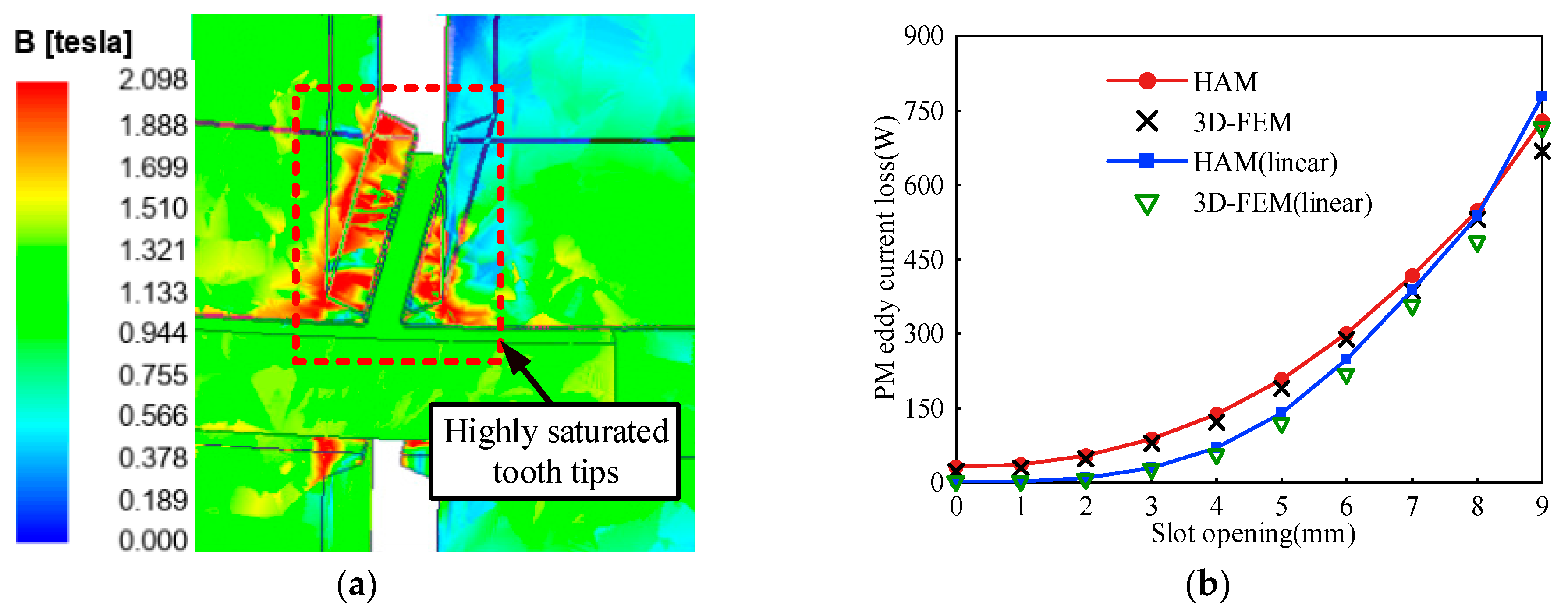
The air-gap permeability harmonics caused by stator slots are a primary source of no-load PM eddy-current losses. Due to the small size of the slot tips, they tend to saturate frequently, as shown in Figure 9a. Ignoring this saturation during calculations can significantly impact the accuracy of the PM eddy-current loss estimation under no-load condition. Figure 9b illustrates the comparison of PM eddy-current loss calculated both with and without considering slot tip saturation across various slot widths. The figure clearly demonstrates a significant difference between the two scenarios, and the HAM can reflect the effect of slot tip saturation.

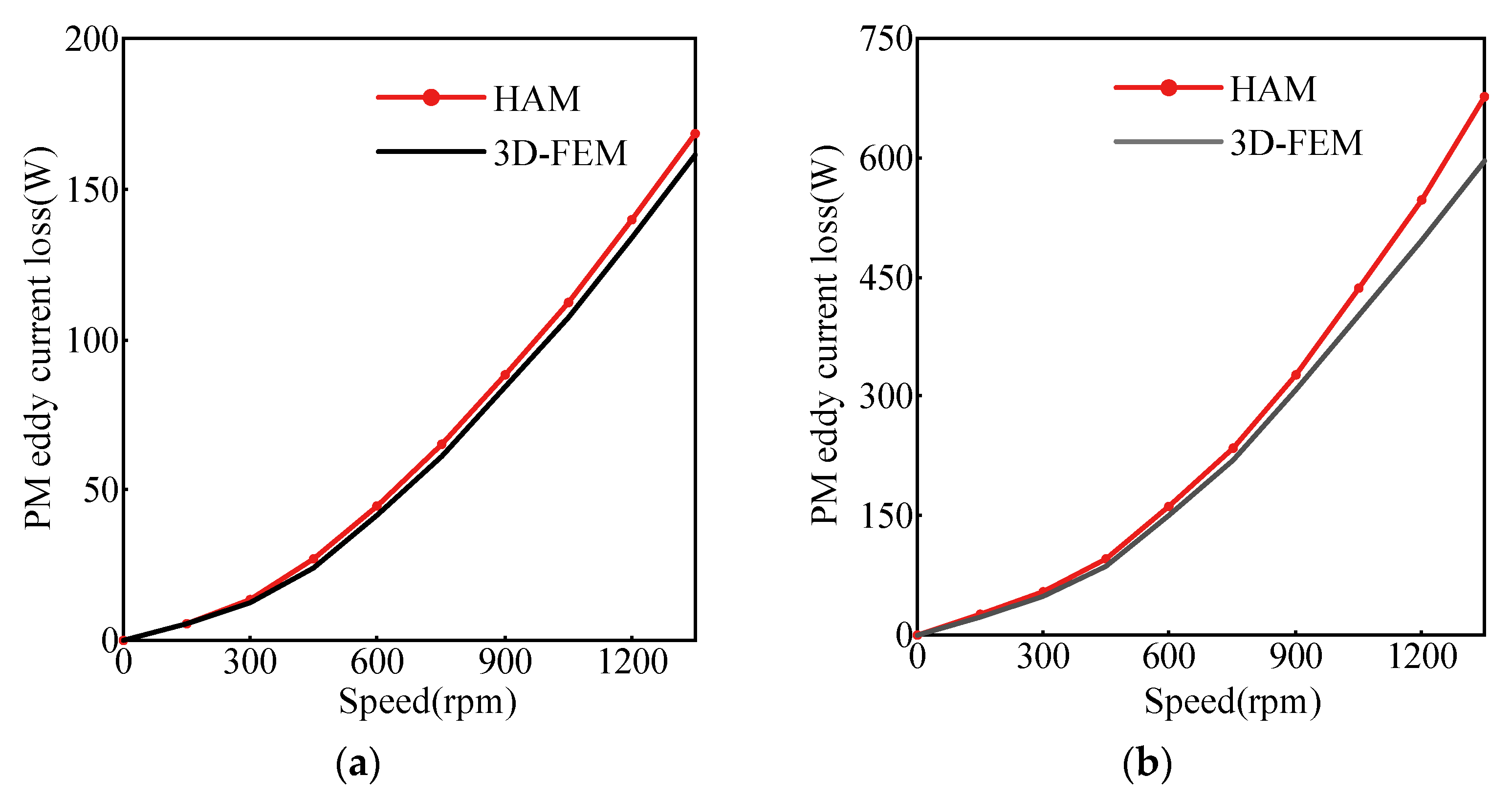
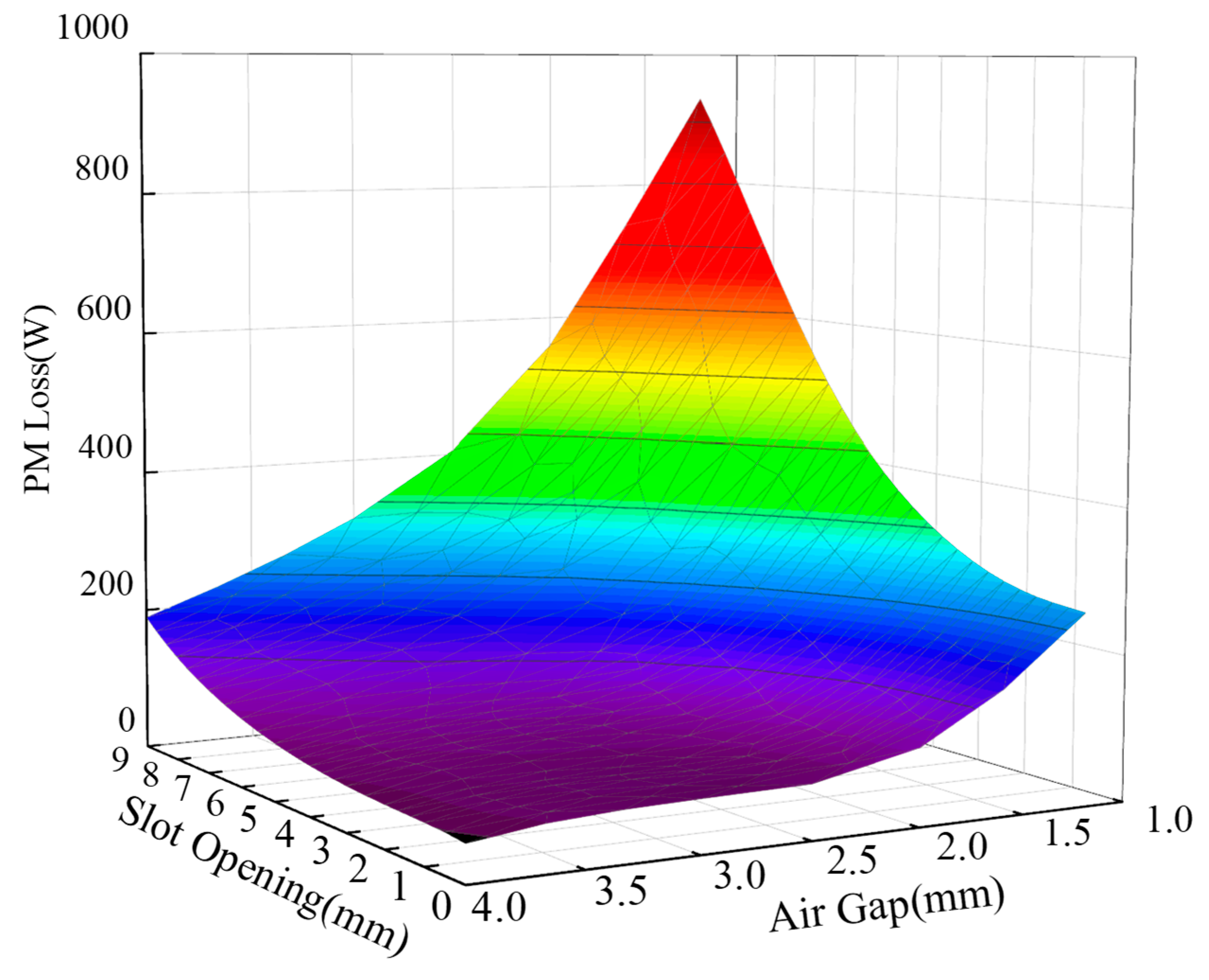
Under load conditions, armature reaction field harmonics is the main contributor to PM eddy-current loss. Figure 9 presents the PM eddy-current loss at different slot opening width and air-gap lengths under rated operating conditions. It is evident that increasing the air-gap length and decreasing the slot width can significantly reduce the PM eddy-current loss. For the AFPMM in Table 1, when the slot width is 3 mm and the air-gap length increases from 1 mm to 4 mm, the eddy-current loss decreases from 321.6 W to 61.7 W, representing an 80.8% reduction. Additionally, reducing the slot width from 9 mm to 0 mm at air-gap length of 1 mm, the PM eddy-current loss decreases from 945.4 W to 267.7 W, a reduction of 71.68%.

From Figure 10, it is evident that reducing the air-gap length and narrowing the slot opening width can effectively decrease the PM eddy-current loss. However, an excessively large air-gap length significantly diminishes the AFPMM’s output torque, which is detrimental to the efficient utilization of both PM and armature winding. In contrast, reducing the slot opening width has minimal impact on the AFPMM’s torque output performance while effectively mitigating the PM eddy-current loss. Therefore, to minimize the PM magnet eddy-current loss, a smaller slot opening width is advisable when designing the AFPMM.

6. Conclusions

In this paper, a HAM for evaluating the PM eddy-current loss in AFPMM is proposed. This model incorporates the saturation effect of the stator core, thereby enhancing the accuracy of calculations. Specifically, it can calculate the air-gap field distribution and evaluate the eddy-current loss under both no-load and load conditions. Compared to traditional methods that do not account for iron saturation, this HAM provides more accurate results for no-load conditions. The validity of the proposed method was confirmed through 3D FEM. Additionally, the impact of air-gap length and slot opening width on PM eddy-current loss was investigated using this HAM. The results indicate that reducing slot width effectively decreases PM eddy-current loss. Moreover, compared to the 3D FEM, the HAM significantly reduces computation time, which facilitates a shorter design period for AFPMM. Importantly, by considering the influence of stator core saturation, the model is also suitable for assessing the electromagnetic performance and PM eddy-current loss under highly saturated conditions such as when the armature current is way above the rated value or operating under overload condition.

References

1. Kampker, A.; Born, H.; Hartmann, S.; Drexler, D.; Franke, J.; Baader, M.; Hahn, R.; Parspour, N.; Schäfer, A.; Pecha, U. Comprehensive Review and Systemization of the Product Features of Axial Flux Machines. In Proceedings of the 2024 1st International Conference on Production Technologies and Systems for E-Mobility (EPTS), Bamberg, Germany, 5–6 June 2024; IEEE: New York, NY, USA, 2024; pp. 1–11. [Google Scholar]
2. Nishanth, F.N.U.; Van Verdeghem, J.; Severson, E.L. A review of axial flux permanent magnet machine technology. IEEE Trans. Ind. Appl. 2023, 59, 3920–3933. [Google Scholar]
3. Schäfer, A.; Pecha, U.; Parspour, N.; Kampker, A.; Born, H.; Hartmann, S.; Franke, J.; Baader, M.; Hahn, R. A review of electromagnetic simulation and modelling approaches for the research on axial flux synchronous machines. In Proceedings of the 2024 1st International Conference on Production Technologies and Systems for E-Mobility (EPTS), Bamberg, Germany, 5–6 June 2024; IEEE: New York, NY, USA, 2024. [Google Scholar]
4. Nishanth, F.N.U.; Van Verdeghem, J.; Severson, E.L. Recent advances in analysis and design of axial flux permanent magnet electric machines. In Proceedings of the 2021 IEEE Energy Conversion Congress and Exposition (ECCE), Virtual Conference, 10–14 October 2021; IEEE: New York, NY, USA, 2021; pp. 3745–3752. [Google Scholar]
5. Zhao, J.; Han, Q.; Dai, Y.; Hua, M. Study on the electromagnetic design and analysis of axial flux permanent magnet synchronous motors for electric vehicles. Energies 2019, 12, 3451. [Google Scholar] [CrossRef]
6. Meier, M.; Strangas, E.G. A Novel Cooling System for High-Speed Axial-Flux Machines Using Soft Magnetic Composites. Energies 2024, 17, 5615. [Google Scholar] [CrossRef]
7. Kang, J.B.; Lee, J.Y.; Lee, J.H. Guidelines for determining the initial shape and specifications of high-speed AFPM based on recent research. Energies 2022, 15, 6099. [Google Scholar] [CrossRef]
8. Wang, H.; Zeng, X.; Eastham, J.F.; Pei, X. Axial flux permanent magnet motor topologies magnetic performance comparison. Energies 2024, 17, 401. [Google Scholar] [CrossRef]
9. Wu, L.J.; Zhu, Z.Q.; Staton, D.; Popescu, M.; Hawkins, D. Analytical modeling and analysis of open-circuit magnet loss in surface-mounted permanent-magnet machines. IEEE Trans. Magn. 2011, 48, 1234–1247. [Google Scholar] [CrossRef]
10. Wu, L.J.; Zhu, Z.Q.; Staton, D.; Popescu, M.; Hawkins, D. Analytical model for predicting magnet loss of surface-mounted permanent magnet machines accounting for slotting effect and load. IEEE Trans. Magn. 2011, 48, 107–117. [Google Scholar] [CrossRef]
11. Ishak, D.; Zhu, Z.Q.; Howe, D. Eddy-current loss in the rotor magnets of permanent-magnet brushless machines having a fractional number of slots per pole. IEEE Trans. Magn. 2005, 41, 2462–2469. [Google Scholar] [CrossRef]
12. Chen, L.; Wang, J.; Nair, S.S. An analytical method for predicting 3-D eddy current loss in permanent magnet machines based on generalized image theory. IEEE Trans. Magn. 2015, 52, 1–11. [Google Scholar] [CrossRef]
13. Vansompel, H.; Sergeant, P.; Dupre, L. A multilayer 2-D–2-D coupled model for eddy current calculation in the rotor of an axial-flux PM machine. IEEE Trans. Energy Convers. 2012, 27, 784–791. [Google Scholar] [CrossRef]
14. Hemeida, A.; Sergeant, P. Analytical modeling of surface PMSM using a combined solution of Maxwell–s equations and magnetic equivalent circuit. IEEE Trans. Magn. 2014, 50, 1–13. [Google Scholar] [CrossRef]
15. Hemeida, A.; Sergeant, P.; Vansompel, H. Comparison of methods for permanent magnet eddy-current loss computations with and without reaction field considerations in axial flux PMSM. IEEE Trans. Magn. 2015, 51, 1–11. [Google Scholar] [CrossRef]
16. Liu, Y.; Wang, C.; Chen, D.; Li, G. A Simple PM Eddy Current Loss Model for Axial Flux Permanent Magnet Machine. In Proceedings of the 2024 IEEE International Magnetic Conference-Short papers (INTERMAG Short papers), Rio de Janeiro, Brazil, 5–10 May 2024; IEEE: New York, NY, USA, 2024; pp. 1–2. [Google Scholar]
17. Jia, L.; Lin, M.; Li, N.; Le, W.; Wu, X.; Chen, Z. Magnetic equivalent circuit framework for an axial flux permanent magnet synchronous machine. In Proceedings of the 2019 22nd International Conference on Electrical Machines and Systems (ICEMS), Harbin, China, 11–14 August 2019; IEEE: New York, NY, USA, 2019; pp. 1–5. [Google Scholar]
18. Derbas, H.W.; Williams, J.M.; Koenig, A.C.; Pekarek, S.D. A comparison of nodal-and mesh-based magnetic equivalent circuit models. IEEE Trans. Energy Convers. 2009, 24, 388–396. [Google Scholar] [CrossRef]
Figure 1. The 1/6 model for the example AFPMM.
Energies 18 02462 g001
Figure 2. The 2D equivalent model.
Energies 18 02462 g002
Figure 3. Stator MEC model.
Energies 18 02462 g003
Figure 4. The calculation flowchart of HAM.
Energies 18 02462 g004
Figure 5. PM equivalence process. (a) The eddy-current distribution within the PM; (b) Schematic diagram of equivalent resistance division for PM.
Energies 18 02462 g005
Figure 6. The equivalent PM resistance network: (a) resistance network for PM; (b) branch j at the middle of resistance network that is located between two sub-circuits; (c) branch j at the edge of resistance network that is only related to one sub-circuit.
Energies 18 02462 g006
Figure 7. Air-gap magnetic flux density distribution with and without saturation. (a) Axial magnetic flux density under no-load; (b) circumferential magnetic flux density under no-load; (c) axial armature reaction field; (d) circumferential armature reaction field.
Energies 18 02462 g007
Figure 8. Comparison of PM eddy-current loss. (a) PM eddy-current loss under no-load condition; (b) PM eddy-current loss under rated current.
Energies 18 02462 g008
Figure 9. PM eddy-current loss under no-load conditions with different slot opening. (a) Diagram of highly saturated tooth tips; (b) comparison of PM eddy-current loss with and without saturation.
Energies 18 02462 g009
Figure 10. PM eddy-current loss under rated load with different slot opening and air-gap length.
Energies 18 02462 g010