The Impact of the Core Laminate Shaping Process on the Parameters and Characteristics of the Synchronous Reluctance Motor with Flux Barriers in the Rotor

Abstract

This article describes the findings of a study that examined the impact of the process of shaping the stator core of a synchronous reluctance motor on its operating parameters. The SynRM motor, with compact geometrical dimensions and a flux barrier rotor, was chosen for this study, for which the technological process of forming the stator and rotor cores may be critical. The numerical results for three types of stator core structures were compared. The first, which is commonly used by academics, has no technological cutouts in the stator. The second type has cutouts for the clamps that hold the core laminates together. The third one has cutouts that allow the core to be positioned inside the motor housing. The research campaign also investigated the effect of partial material structure degradation caused by core laminate shaping on motor operation parameters. As a consequence of the computations, the characteristics and motor parameters were compared, including torque ripple, stator core loss, and motor efficiency. It has been demonstrated that, in the case of SynRM motors with relatively small geometric dimensions, technological cutouts caused by the shaping of stator core laminates can drastically influence the motor’s characteristics.

1. Introduction

Synchronous reluctance motors are an attractive, sustainable, and future-oriented electric drive because of their simple and inexpensive rotor design and lack of use of rare raw materials (NdFeB magnets). The torque generated is determined by the reluctance difference between the rotor’s direct (d-axis) and quadrature (q-axis) components. It is generally known that rotor design greatly influences torque and its pulsations. Torque pulsations are a disadvantage of this type of motor; therefore, many scientists are working on optimizing rotor shape, with a particular emphasis on rotors with flux barriers. Torque pulsations can exceed 100% of the average torque generated by the motor in poorly optimized solutions, limiting the range of applications for this type of synchronous motor.

In general, the design and optimization of SynRM motors involves the selection of the number of flux barriers and their dimensions, as well as the shape of the barrier end located near the magnetic bridge. Many studies in the literature describe techniques for optimizing rotor shape to increase average torque while reducing torque pulsation. It is worthwhile to mention the research conducted by various groups of scientists, which indicates ways to increase average torque density while reducing torque ripple. This goal can be met by optimizing the number, shape, position, and size of flux barriers in the rotor or by incorporating additional permanent magnets into the rotor [1,2,3,4,5,6,7,8]. The results show that the solutions used are highly effective. For example, torque ripple can be reduced from 200% of average torque to 10% [3]. Other unconventional methods of reducing torque ripple are also mentioned in the literature. Good examples are studies using mirror-asymmetrical flux barriers in the rotor, which reduced torque ripple to 2.8% while maintaining high motor efficiency [9,10,11]. The use of various types of curves (quadratic curves and B-spline curves) is a distinct field for determining the optimal shape of flux barriers in terms of torque ripple reduction [12,13,14,15]. For example, the authors reported a threefold reduction in torque ripple when B-spline curves were used instead of a rectangular form for the barrier ends [13]. Some of the research papers mentioned above deal with motors with relatively small geometrical dimensions, or the optimal width of the flux barriers is small (e.g., 0.3–0.7 mm), or the barriers must be manufactured with a precision of 0.1 mm [3,4,11,16]. Despite the core’s relatively small geometrical dimensions, these studies did not address the issue of changing motor parameters due to changes in the properties of the material being cut. Although the core’s relatively small geometrical dimensions may serve as a good starting point for discussions on this topic. A good example is the motor described in [11], which has a 44.7 mm external core diameter.

The selection of appropriate techniques for designing flux barriers in the rotor of a reluctance motor is a fundamental research problem that has been addressed for many years. Examples of research in this area are shown above. In turn, the effect of manufacturing processes, such as laminate cutting or core assembly, on motor performance is a separate area of research. Popular core assembly technologies (clamping, welding, or interlocking) and cutting technologies (punching, laser cutting, spark erosion, or water jet cutting) should be considered here. Finally, extensive research should be conducted to determine the impact of the chosen cutting technology on changes in local material properties. This research should result in a thorough understanding of the impact of applied technological processes on changes in motor parameters. The available literature contains a significantly smaller number of studies in this area. Among them are works that consider technological process tolerance when determining the parameters and operating characteristics of reluctance motors. This issue was investigated and described in [17,18]. In [17], the authors investigated the effect of placing flux barriers in the rotor, which were cut with laser cutting technology with a tolerance of ±0.1 mm. According to the study’s findings, the motor’s average torque changed by 0.5%, while torque ripples increased by 3%. Another group of researchers investigated this issue by considering a much broader range of dimensional changes, such as the dimensions of flux barriers and stator slots [19]. Additionally, statistical tolerance analysis was used in the study. This work resulted in the calculation of statistical distributions for both torque ripple and average torque. The study found that, in the worst-case scenario, torque ripples can change by 40%, and average torque by 20%. In turn, an attempt to consider the impact of the punching process on the average torque and its ripple was made in [20]. Based on the observations made, the authors came to the correct conclusions, namely that changes in material properties near the cut edge are influenced by mechanical stresses “generated” by the cutting process. Another correct observation was that this impact is proportional to the flux density and decreases as induction increases. The conducted study focused on an SyRM motor with a rotor that had three U-shaped flux barriers. The study found that accounting for mechanical stresses reduced the average torque by 5% and torque pulsation by 2–3%. After accounting for stress-induced material changes, large fragments of material in all flux barriers showed induction above 2T, whereas the stator yoke was practically unsaturated. This working condition caused minor changes in average torque and torque ripples. Further in-depth analysis was impossible due to the poor description of the FEM model and simulation conditions. In turn, ref. [21] provides a more detailed analysis of the effect of laser cutting on flux barrier material property change. In this case, the investigation focused on a rectangular sample rather than on a motor. The authors investigated the distribution of mechanical stresses and the resulting changes in material magnetic permeability of a rectangular sample with a flux barrier cut in the center. The study’s findings confirmed the well-known fact that, when induction exceeds 1.6 T, permeability changes are weakly affected by mechanical stresses. Simultaneously, the authors observed that, after exceeding a certain stress level, the material’s permeability stopped decreasing and even slightly increased.

This paper provides a comprehensive review of research findings on modeling techniques for the flux barriers’ shape in the SynRM rotor. The methods and techniques used for modeling flux barriers are well understood and documented, but the effect of the cutting and forming laminations process on changes in SynRM parameters is not fully understood or recognized. Thus, the author discusses the key aspects of lamination shaping and their impact on motor operating parameters. This article attempts to fill that gap by describing the author’s research on the effects of the cutting process (punching and laser cutting) and stator core shaping on parameters of the reluctance motor. The research findings are significant in terms of the needs of electric motor designers (including SynRM) who work on motors with relatively small geometrical dimensions. The proposed procedure, which includes both the construction of the FEM model and the method for determining the material properties of individual zones of the model, is practical.

This study’s subject was a reluctance motor with relatively small dimensions, on which the technological process was expected to have a visible impact on the motor parameters. The term “SynRM motors with relatively small geometric dimensions” used in the abstract and article content refers to SynRM motors with an external core diameter of less than 100–150 mm. In this case, the magnetic circuit fragments, such as the stator or rotor yoke, stator teeth, or flux barriers in the rotor, have widths comparable to the width of the zone with material properties changed by the cutting process. According to the author’s and other scientists’ research, the width of such a zone varies depending on the material and cutting technology used, and can be estimated to be 2–3 mm. In this case, the material changes caused by the cutting process must be considered when designing the motor. It is unnecessary to account for material changes in motors with yoke and teeth dimensions that are much larger than the width of the aforementioned zone. A separate issue is the presence of technological cutouts within the stator core. If the depth of such a cutout exceeds 10–15% of the width of the magnetic circuit fragment, this must be considered during the design process.

The goal of this research is to demonstrate the importance of considering changes in material properties (due to cutting), as well as the shape of the core laminates, when determining the characteristics and parameters of the SynRM motor. This will be accomplished in several stages. The first step is to take magnetic measurements on strips of various widths. They will serve as the data source for the method of determining the local material properties. The local material properties will be used to calculate the equivalent material properties of the FEM model zones. Simulations will then be run using the FEM model. The simulation results will determine the level of torque ripple, harmonic content in the torque waveform, core losses, and motor efficiency.

The article is organized as follows: introduction, magnetic measurements and determination of local properties of materials subjected to punching or laser cutting process, the scope of analysis of the SynRM motor and its FEM models, results of performed numerical simulations, discussion, and conclusions.

2. Magnetic Measurements and Determination of Local Properties of Material Subjected to Punching or Laser Cutting

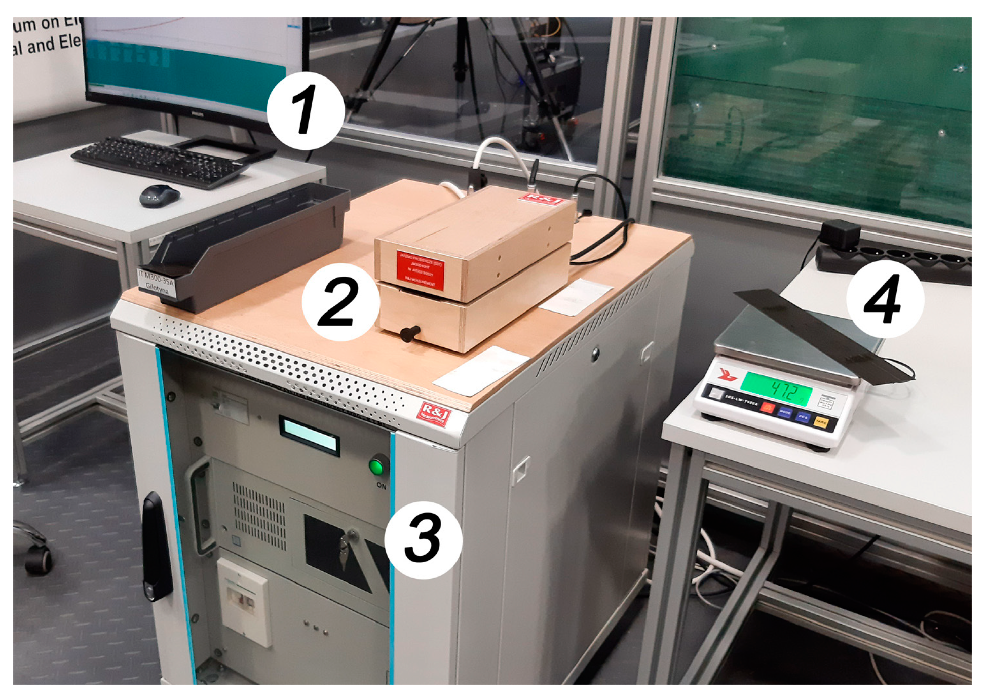
2.1. Magnetic Measurements with the SST System

The measurements were performed on the low-loss M300-35A material. A commercial SST (Single Strip Tester) was used to evaluate the material properties of rectangular strips with a total width of 60 mm (see Figure 1). Strips with widths of 4, 6, 7.5, 10, 20, 30, and 60 mm were tested to determine the material’s magnetization and specific iron loss curves. In each case, the appropriate number of strips was chosen so that their total width was close to 60 mm, making the best use of the measuring yoke’s width. For example, 12 strips with a width of 5 mm were used simultaneously. A 60 mm wide strip was also cut with a water jet, keeping the material’s original properties near the cut edge. The material properties of this strip were used for reference. The remaining strips, which varied in width from 4 to 30 mm, were punched and laser cut. More data on the measuring station and the laser parameters used in cutting can be found in [22]. The measurement results from the aforementioned strips were used as a data source for the author’s method of determining local material properties as a function of distance from the cut edge.

The measurements were performed at flux densities ranging from 0.05 to 1.7 T. For larger inductions, appropriate extrapolations of the measured material properties were made. The used SST system controlled the shape of the voltage induced in the measuring winding (and thus the shape of the induction waveform) by selecting appropriate instantaneous excitation current values. The use of software tools allowed the process to be automated. The measurements yielded two families of curves, as follows: B = f(H) for magnetization and p = f(B) for specific iron loss. It is worth noting that the average B_AV,max induction across the strip cross-section was consistently measured. The average induction for a d-width strip is calculated using local magnetic permeability and a constant value of H_max magnetic field strength on the strip’s surface, as follows:

$$B_{AV,max}={\displaystyle \frac{2}{w}}{\int }_0^{{\displaystyle \raisebox{1ex}{$w$}\!\left/ \!\raisebox{-1ex}{$2$}\right.}}{H}_{max}{\mu }_0{\mu }_r\left(x\right)dx={\displaystyle \frac{2}{w}}{H}_{max}{\mu }_0{\int }_0^{{\displaystyle \raisebox{1ex}{$w$}\!\left/ \!\raisebox{-1ex}{$2$}\right.}}{\mu }_r\left(x\right)dx$$

(1)

where the B_AV,max maximum induction value is calculated as an average over the strip’s cross section, H_max is the maximum magnetic field strength on the surface of the strip, w is the strip width, µ_r(x) is the actual material relative magnetic permeability at the x distance from the cut edge, and µ₀ is the vacuum permeability.

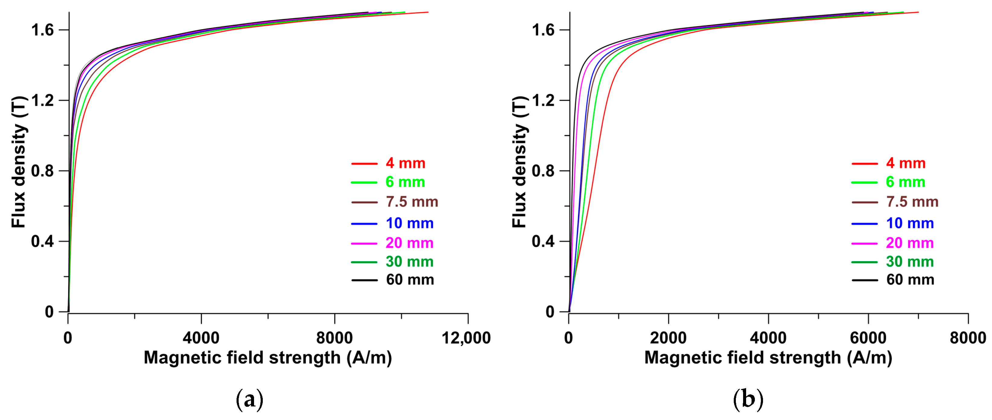
Figure 2 and Figure 3 present the results of the measurements conducted on the M300-35A material. They are presented in the classical format, with the family of magnetization curves plotted as a function of magnetic field strength and the family of specific iron loss curves plotted as a function of average induction in the strip cross-section. 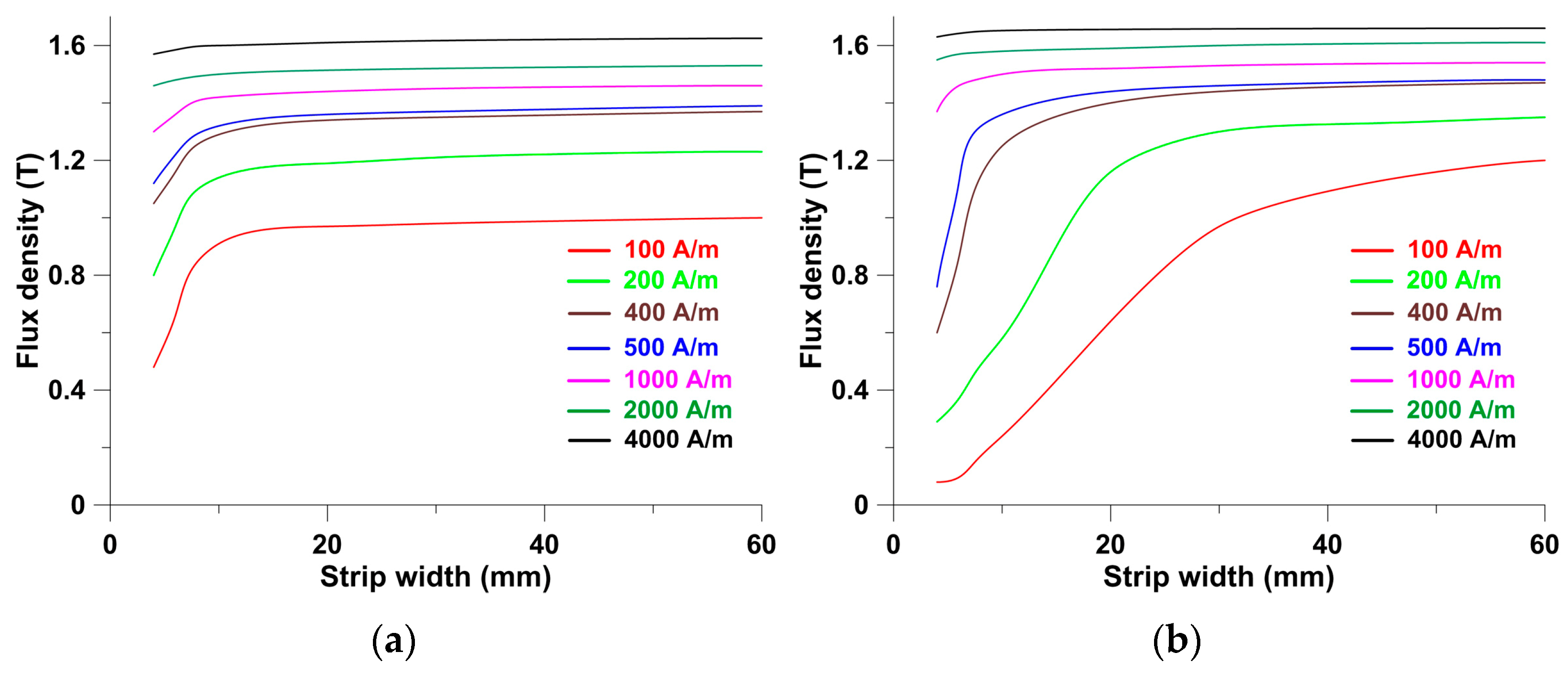Individual magnetization curves in Figure 2 and specific loss curves in Figure 3 are color-coded to correspond to the previously mentioned strip widths (for example, red for a 4 mm wide strip and black for a 60 mm wide strip). These findings are presented in a new format, allowing for further investigation. The families of average flux density curves and specific iron loss curves were plotted as a function of strip width while the magnetic field strength on the strip surface remained constant (see Figure 4 and Figure 5). A similar procedure was used for each curve in Figure 4 and Figure 5. In this case, the results are shown for magnetic field strengths of 100, 200, 400, 500, 1000, 2000, and 4000 A/m. It should be remembered that the curves contain aggregated values of material permeability and specific iron loss, which were used to calculate the local material properties.

2.2. Method for Determining the Local Properties of Ferromagnetic Material

Local magnetic induction was reproduced using the measurement results (flux density averaged over the strip cross-section) shown in Figure 4 as a family of curves B = f(w), where w is the width of the rectangular strip being tested. As mentioned earlier, each of these curves was plotted for a particular maximum magnetic field strength on the strip surface. Thus, they are the curves that describe the material’s average magnetic permeability as a function of strip width. It should be mentioned that the M300-35 material was tested in another measurement campaign. As a result of the campaign, several test results for this material were presented, including curves that describe both local (reproduced) and average (measured) induction [23]. As stated in (1), the magnetic induction averaged over the strip cross-section for a given magnetic field strength can be directly related to the distribution of local induction by using the following relationship:

$$B_{AV,max}\left(w,H_{max}\right)={\displaystyle \frac{1}{w}}{\int }_0^w{B}_{loc,max}\left(x,H_{max}\right)dx$$

(2)

where B_AV,max (w, H_max) is the measured maximum flux density value for a strip of the w width and B_loc,max (x, H_max) is the maximum value of local flux density at the x distance from the cut edge.

By dividing both sides of Equation (2) by H_max, we can determine the relationship between the strip material’s measured average magnetic permeability and its local magnetic permeability at a distance x from the cut edge. As a result, we can express the following relationship:

$${\mu }_{AV}\left(w,H_{max}\right)={\displaystyle \frac{1}{w}}{\int }_0^w{\mu }_{loc}\left(x,H_{max}\right)dx$$

(3)

As previously noted, the cutting process changes the magnetic permeability of a portion of the material. This is well described in the literature, as is the relationship that approximates this change. The exponential relationship used to describe these changes is frequently assumed [24,25]. In [23], the author proposed the following relationship for modeling changes in local magnetic permeability (for a given magnetic field strength), which was used in this study:

$${\mu }_{loc}\left(x\right)=a+b·\left(1-e^{\left(-x·tt\right)}\right)$$

(4)

where a, b, are the fitting parameters found in the error minimization process between the approximation (using Equation (3)) and the measurement data, and tt is the characteristic material parameter depending on the distance x.

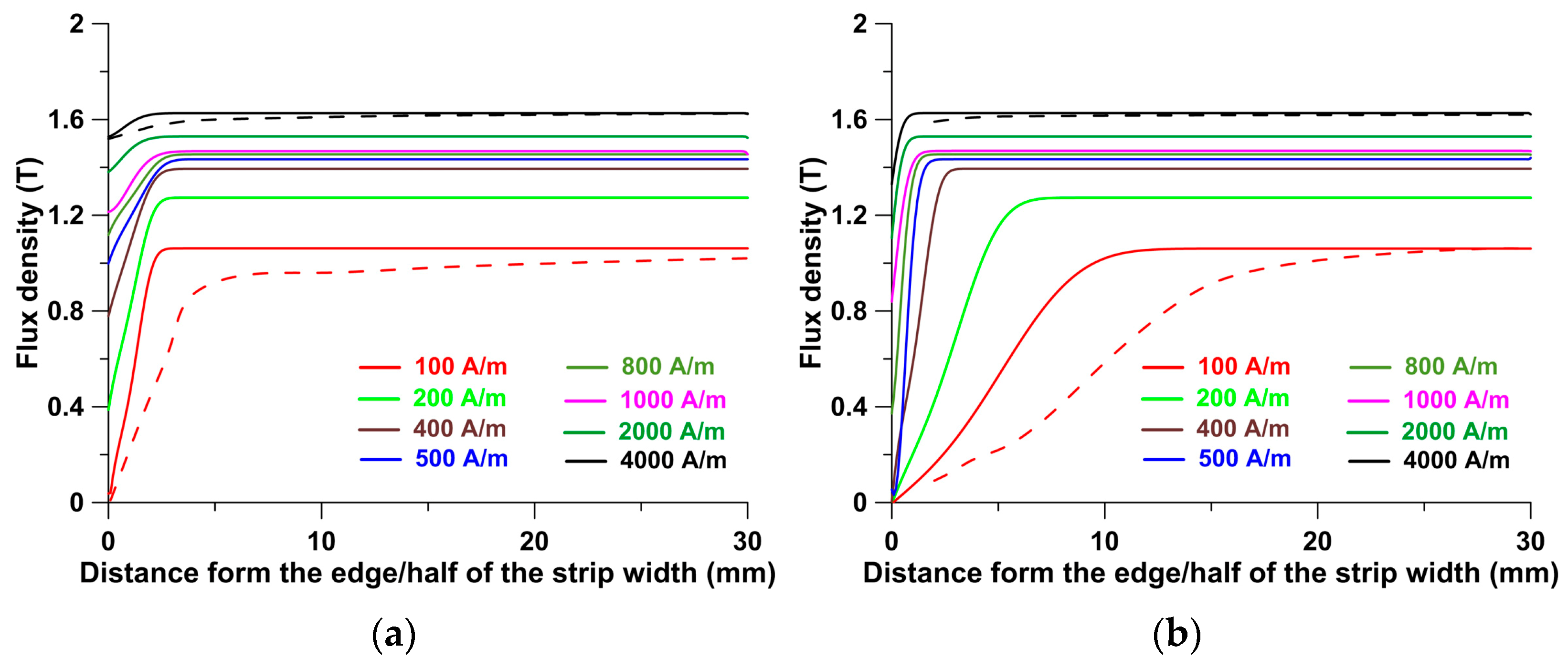
According to the author’s findings in [23], changes in local magnetic induction occur at distances of up to 2–3 mm from the cut edge (guillotine) and up to 10 mm (laser). The range of these changes is also determined by the strength of the magnetic field. This range is wider for relatively low magnetic field strengths than for relatively high magnetic field strengths. This is especially noticeable in the case of laser cutting.

For various magnetic field strengths, a family of color-coded local magnetic induction (local magnetic permeability) curves was determined as a function of distance from the cut edge (see Figure 6). In this case, the results are presented for the following magnetic field strengths: 100 (marked in red), 200, 400, 600, 800, 1000, 2000, and 4000 (marked in black) A/m. Following that, by selecting a specific distance from the edge, the local induction values for the indicated magnetic field strengths were read. In this way, a local magnetization curve was obtained for the portion of the material located at that distance. Figure 6 compares several reconstructed local magnetization curves with two measured curves (obtained for average induction).

A separate issue is determining an expression that describes the change in specific iron loss as a function of distance from the cut edge. In this scenario, we can write the following relationship between the measured average specific iron loss and the local specific iron loss:

$$p_{AV}\left(H_{max}\right)={\displaystyle \frac{1}{w}}{\int }_0^w{p}_{loc}\left(H_{max}, x\right)dx$$

(5)

where p_AV(H_max) is the measured specific iron loss, averaged over the strip cross-section (volume), and p_loc(H_max,x) is the local specific iron loss of the material, at the x distance from the cut edge.

As previously stated, we accept the exponential nature of changes in the magnetic permeability of the cut material as a function of distance from the cut edge, based on the author’s own research and that of others. In the literature, we find a similar exponential relationship between local iron loss and distance from the cut edge, as follows [24]:

$$p_{loc}\left(B_{max}\left(H_{max},x\right),x\right)=c·\left(1+e^{-dx}\right)·B_{max}^2\left(H_{max},x\right)$$

(6)

where p_loc(B_max(H_max,x), x) is the local specific iron loss, B_max(H_max,x) is the maximum flux density at H_max magnetic field strength, and the x distance from the cut’s edge and c, d are the fitting parameters.

The above approach is acceptable, though specific iron losses are usually defined by a three-component dependence. These include the specific hysteresis loss, the specific classical eddy current loss, and the specific excess loss. Some individual components in this approach are a function of magnetic induction at a power other than two. In the literature, we find the following relationship, which describes the local specific iron loss in a partially damaged material [26]:

$$p_{loc}\left(x\right)=a_1\left(x\right){B_{max}\left(x\right)}^{2}f+a_2\left(1+a_3{B_{max}\left(x\right)}^{a4}\right){B_{max}\left(x\right)}^2{f}^2+a_5{B_{max}\left(x\right)}^{1.5}{f}^{1.5}$$

(7)

where a₁(x) is the hysteresis coefficient being dependent on distance from the cut’s edge; a₂, a₃, a₄, and a₅ are material coefficients; and f is the frequency.

The above-mentioned dependence includes coefficients determined for the material using the commonly used method of iron loss component separation. Another group of researchers tried to find a similar relationship using modified classical dependence [27].

$$p_{loc}{\left(x\right)=a}_1\left(x\right)B_{max}^{\alpha }f+a_2{B}_{max}^2{f}^2+a_3{B}_{max}^{1.5}{f}^{1.5}+a_4{B}_{max}^{a_5+2}{f}^2$$

(8)

The specific hysteresis loss, which is the first component of Equations (7) and (8), is determined by induction to the power of two in Equation (7) and by the power of α in Equation (8). Both approaches are acceptable because they only differ in the way the coefficient a₁(x) is calculated. In the first case, the level of magnetic induction determines it, whereas, in the second, it is constant. Taking into account the author’s own findings, as well as those of other groups, it was decided to use the following relationship to define the material’s local specific iron loss:

$${p\left(x\right)}_{loc}=k\left(x\right)c_h\left(B_{max}\left(x\right)\right){B_{max}\left(x\right)}^{2}f+c_e{B_{max}\left(x\right)}^2{f}^2+k\left(x\right)c_{ex}{B_{max}\left(x\right)}^{1.5}{f}^{1.5}$$

(9)

where k(x) is the increase factor representing the change in local material properties resulting from the cutting process, c_h(B_max(x)) is the hysteresis coefficient being dependent on the magnetic induction level, c_e is the classical eddy current coefficient, and c_ex is the excess loss coefficient.

According to the research, the observed increase in hysteresis loss and excess loss components is caused, among other things, by internal stresses. Furthermore, the mentioned increase is related to changes in material microhardness, grain structure destruction, and, most importantly, an increase in dislocation density in the crystalline structure. As a result, the values of both iron loss components vary with distance from the cut edge. These findings are supported by both the author’s own research and that of other authors [23,28,29,30,31,32]. As a consequence, in the adopted iron loss model (9), the hysteresis and excess loss components were assumed to increase at the same rate. Their increase is described by the factor k(x), which has an exponential relationship with the distance from the cut edge, as follows:

$$k\left(x\right)=1+a·e^{-{\displaystyle \frac{x}{EW}}}$$

(10)

where a is a fit coefficient and EW is the effective width of the damaged zone, which can be determined from the exponential approximations of the induction curves presented in Figure 5. The a coefficient for the tested material is 2.2 for punching and 3.1 for laser cutting. The EW coefficient for punching is 1.40 mm (regardless of magnetic field strength), while, for laser cutting, it is 2.47 mm (for magnetic field strengths greater than 400 A/m). Lower field strengths increase its value, reaching 3.50 mm for a magnetic field strength of 100 A/m.

Equation (9) contains the factor c_h(B_max(x)), whose dependence on flux density was determined using quasi-static iron loss measurements at 5 Hz. A water-cut strip 60 mm wide was used for this purpose. The water cutting prevented internal structural damage. The experiments carried out resulted in the following relationship:

$$c_h\left(B_{max}\right)=0.0084+0.0051/B_{max}^2$$

(11)

The remaining material coefficients in the relationship (9), c_e and c_ex, were calculated for the undamaged material (a 60 mm wide water-cut strip). In that case, the measurements were performed by varying the frequency from 5 to 400 Hz and minimizing the curve approximation error (12).

$$p/f-c_h\left(B_{max}\right)B_{max}^2=c_e{B}_{max}^{2}f+c_{ex}{B}_{max}^{1.5}{f}^{0.5}$$

(12)

The coefficients obtained as a result of the performed activities are as follows: c_h(1T) = 0.0135 Am⁴/Vskg, c_e = 57.2 × 10⁻⁶ Am⁴/Vkg, c_ex = 488 × 10⁻⁶ Am³/V^0.5skg.

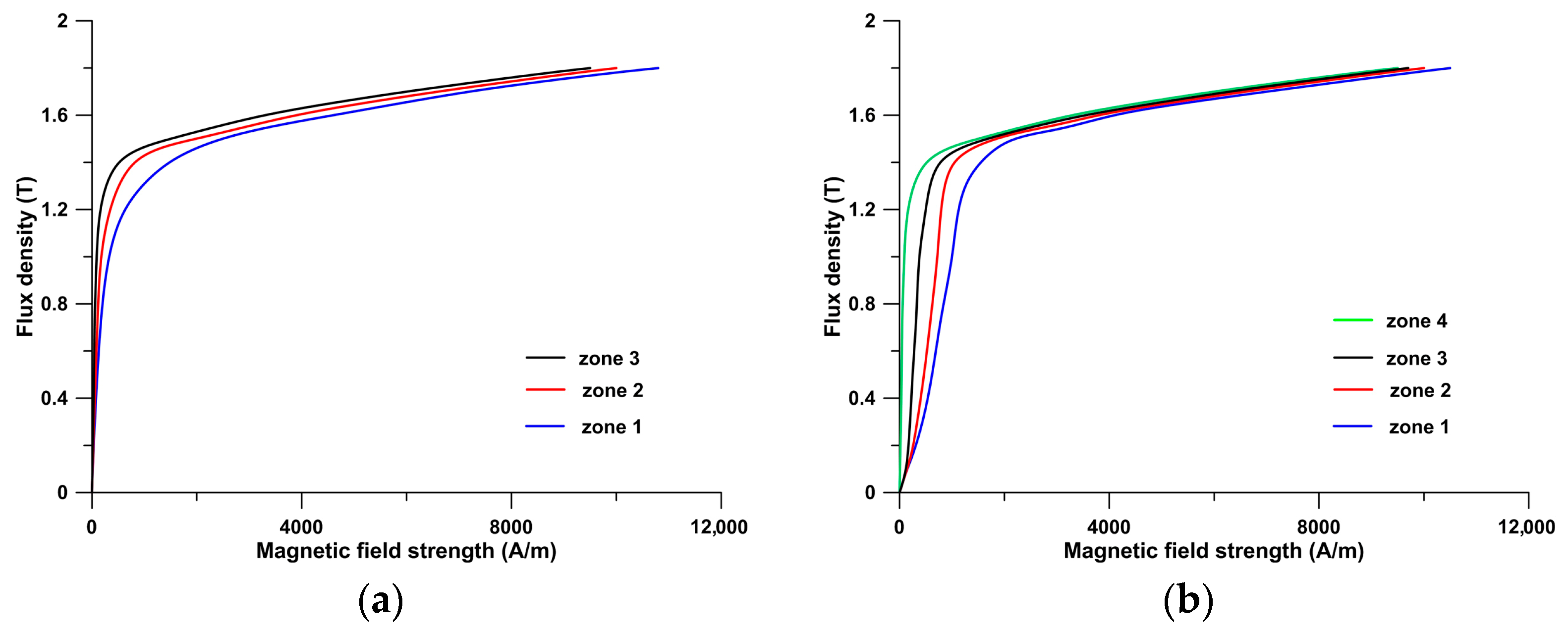
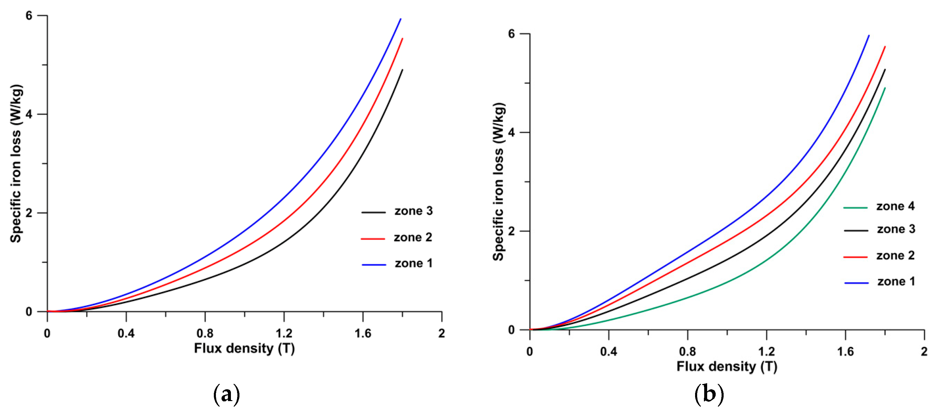
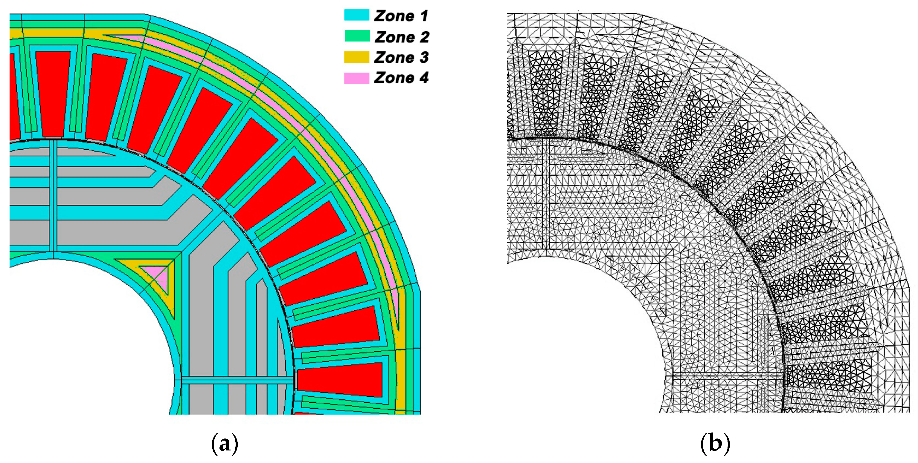
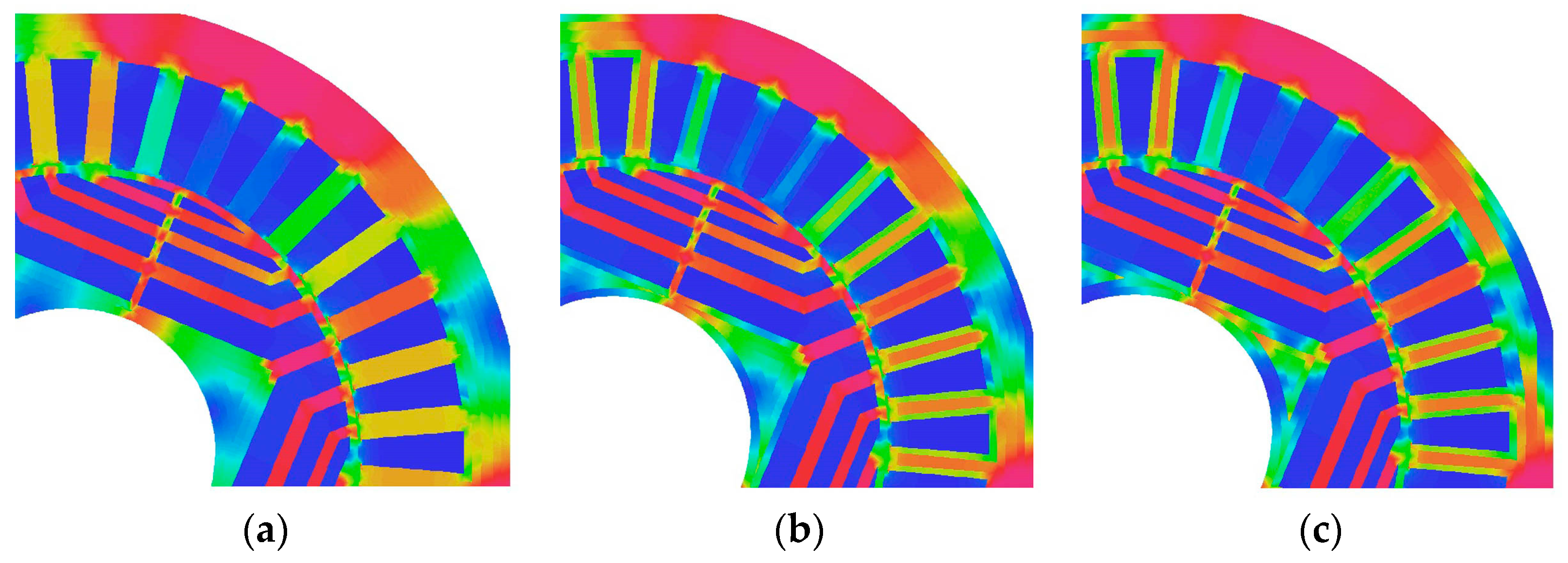
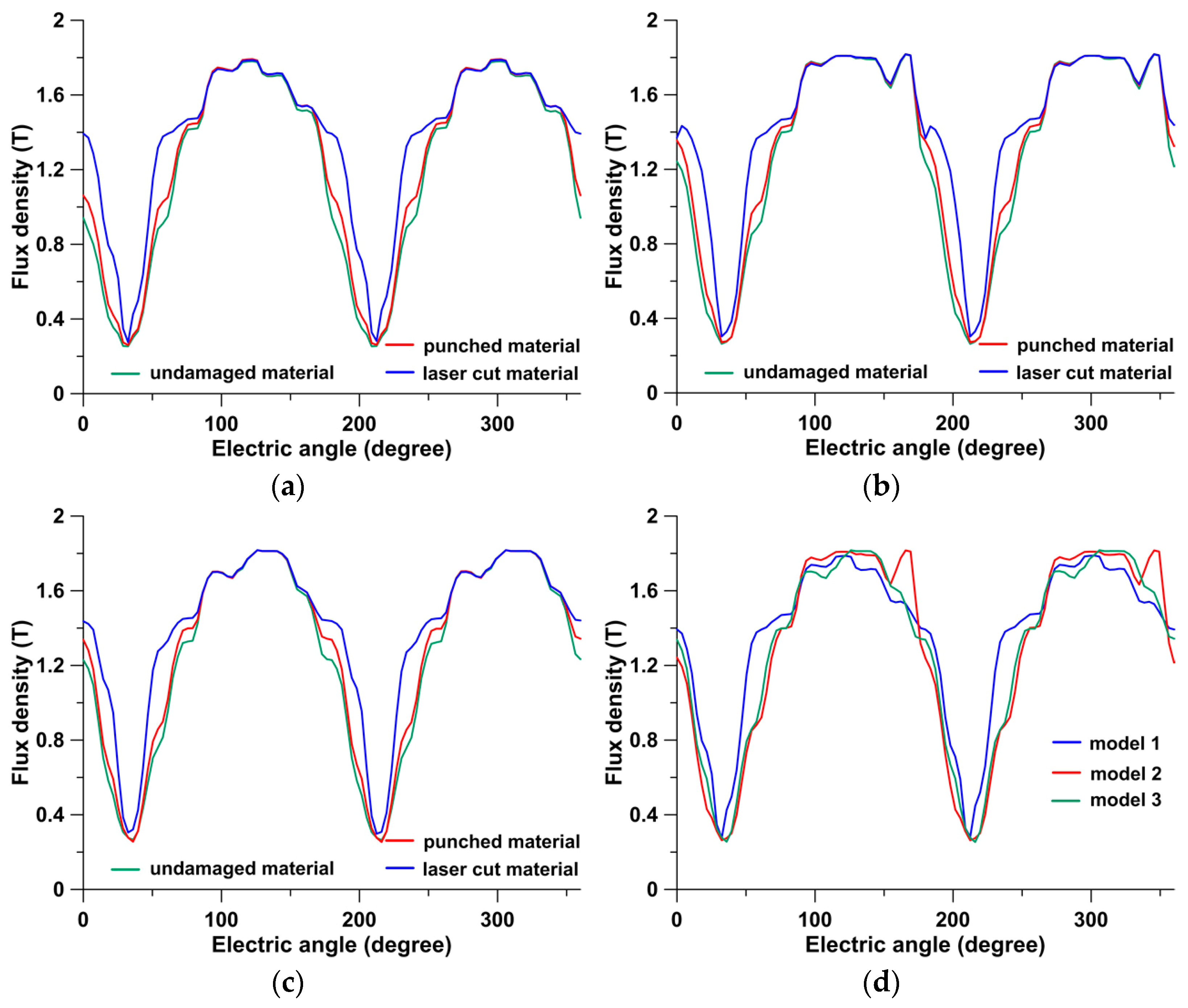
The previously determined local curves of magnetization and specific iron loss were used to calculate curves for materials with equivalent properties. These materials were located in different zones of the FEM model. The FEM model defined three zones of different materials, each located at various distances from the cut edge, as follows: 0–1 mm, 1–2 mm, and 1–3 mm. For zones located at greater distances, the material property was assumed to be similar to that of undamaged material. The FEM model for punched material will then assume two zones with different materials, each described by equivalent properties, namely zone 1, extending from 0 to 1 mm from the cut edge, and zone 2, extending from 1 to 2 mm. The material in zone 3 that extended more than 2 mm from the cut edge was considered undamaged. In the case of laser-cut material, three zones (with equivalent material properties) have been assumed, as follows: zone 1 extending from 0 to 1 mm from the cut edge, zone 2 from 1 to 2 mm, and zone 3 from 2 to 3 mm. The undamaged material was considered for distances greater than 3 mm (zone 4). Magnetization curves (Figure 7) and specific iron loss curves at 50 Hz (Figure 8) were calculated for each zone.

3. The Scope of Analysis of the SynRM Motor and Its FEM Models

3.1. Analyzed Shapes of the Stator Sheets

A four-pole SynRM motor with a rated power of 120 W was tested. Its stator design is based on that of a mass-produced line-start reluctance motor with a standard salient-pole rotor and no flux barriers. In this study, the tested motor with a flux barrier rotor retained the main dimensions of the stator sheets, and the stator windings remained unchanged. The original rotor was replaced by an experimental flux barrier rotor. The original motor was 60% efficient and consumed 0.6 A at the rated load. It should be noted that the core elements are small enough so that the effect of the laminate cutting process on changes in the material portion’s properties must be considered.

Table 1. The main geometric dimensions of the tested 120 W motor.

Parameter	Values
Stator outer diameter	106 mm
Stator inner diameter	68 mm
Stator tooth width	3.6 mm
Stator yoke height *	7.3 mm
Air-gap length	0.22 mm
Length of stator core	35 mm
Number of slots in stator	26
Number of poles	4
Number of rotor barriers/poles	4
Stator slot fill factor	0.67
Material	M300-35
Stator winding connection	Delta

* The stator yoke height is the distance between the outer edge of the stator core sheet and the bottom of the stator slot. It applies to the model without any additional structural cutouts in the stator core.

contains the main geometric dimensions.

As previously stated, the tested motor had an experimental flux barrier rotor with the same outer and inner diameters as the original motor (see Figure 9). The shapes and sizes of the barriers were not optimized. Their number and dimensions were determined by analyzing the results of studies described in the literature presented in the introduction. This approach is justified by the purpose of the research described in this article, which is to investigate the impact of the manufacturing process on the parameters of the SynRM motor. The height of the bottom flux barrier was assumed to be 3.5 mm. The next barriers were 2.5 mm and 1.5 mm high, with the top flux barrier standing at 1.2 mm high. Additionally, the tangential and radial ribs were both 1 mm wide.

The use of technological cutouts in the stator package may be required during the core assembly process prior to installation in the housing. The stator package, including the windings, must be one piece. The following four laminate integration technologies are available for this purpose: gluing, interlocking, clamping, and welding. Each of these integration technologies has its limitations. Gluing, for example, reduces the amount of active material in a package of a certain length. Interlocks mechanically weaken the package while destroying the material around it. Clamping necessitates the presence of suitable cut-outs in the stator core, reducing the yoke’s active cross-section. Welding is the most invasive process, causing material deterioration near the weld. A separate issue is the method of installing the core inside the housing, which is especially important with short cores. In this case, additional cutouts are created near the stator pack’s outer edge. The study described in this paper focused on the effect of clamping cutouts, as well as the effect of cutouts required for mounting the core in the housing (Figure 10).

3.2. FEM Models

Three FEM models were created, each with a different stator geometry (Figure 10). Model 1 has no technological cutouts in the stator core (Figure 10a), which is consistent with other researchers’ descriptions of SynRM motor models. Models 2 and 3 have stator cores with technological cutouts, as shown in Figure 10b,c, respectively. A comparison of the computer simulation results for these models will clearly demonstrate the effect of technological cutouts on motor parameters. Each of these models may account for the presence of damaged material zones caused by shaping the stator and rotor lamination geometry. Section 2.1 discussed the location and number of these zones, which differed depending on the cutting technology used. This topic was discussed in relation to the method for determining equivalent material properties in specific zones of the stator and rotor cores. The computer simulation results obtained for Model 1, which do not account for changes in material properties, will be used to compare with other obtained simulation results. Based on the available material test results, it is known that changes in material properties caused by cutting occur continuously in space. However, incorporating this fact into the FEM model necessitates the use of specialized software tools. The author used professional FEM software that does not permit interference with the software code. That is why this approach cannot be used. As a result, the zones mentioned in Section 2.1 were created with a width of maximum 1 mm in the FEM models used, as shown in Figure 11a. It was assumed that the distance from the cut edge determines the degree of material degradation caused by the cutting process. Thus, the FEM model’s number of zones is proportional to the actual width of the magnetic circuit fragment. For example, the stator tooth is 3.6 mm wide. The FEM model will, therefore, include zone 1 with a width of 1 mm and zone 2 with a width of 0.8 mm. For the stator yoke, the FEM model includes zones 1, 2, and 3, each 1 mm wide, as well as zone 4, whose width is determined by the complement of the yoke width. The material in these zones is described by equivalent material characteristics, as discussed in Section 2.2. The built FEM models had a denser mesh in critical areas, like the air gap, stator teeth, and rotor ribs (see Figure 11b). The air gap was divided into three layers. This allowed for the use of a solver that took into account the rotor’s free rotation as a result of the generated reluctance torque. The solver thus permitted free rotor positioning relative to the stator winding’s magnetic field vector, which corresponded to the given average load torque. The FEM models also included circuit equations. In this manner, the simulation took into account that the stator windings were powered by the rated sinusoidally alternating voltage.

4. Results of Performed Numerical Simulations

The research campaign focused on three FEM models of a low-power synchronous reluctance motor, each with a unique stator core geometry. The modelled motor was composed of an experimental rotor with four flux barriers and a stator adapted from a commercial salient pole reluctance motor. It was expected that the non-optimized shape of the flux barriers, combined with the single-layer stator winding, would contribute significantly to torque ripple. Computer simulations confirmed this expectation. Due to the study’s goal, the decision not to address the shape optimization of the flux barriers in this campaign has been maintained. Computer simulations were conducted at the rated voltage and load of 0.8 Nm. Two aspects of the impact of the stator and rotor core manufacturing processes on motor performance were studied. The first one was concerned that a portion of the laminate material had been damaged during the cutting process. The second one addressed the effect of the stator yoke’s variable width caused by the presence of technological cutouts. To distinguish between the models, the following terminology was used: model_1—the stator core has no technological cutouts; model_2—the stator core has cutouts for mounting the core in the housing; and model_3—the stator core has cutouts for clamps that join the stator core laminates.

Calculations for each type of FEM model were carried out in three ways. The first one ignored material destruction. The second took into account the destruction of a portion of the material due to punching, and the third took into account the destruction caused by laser cutting. The destruction of a material was considered by defining three or four zones with various materials, as described in Section 2.2 and illustrated in Figure 11a. Figure 12 shows the numerical simulation results for the spatial distributions of the instantaneous flux density in model_1, Figure 13 depicts distributions in model_2, while Figure 14 depicts distributions in model_3. In turn, Figure 15 compares the instantaneous flux density distributions along a path located at the mid-height of the stator yoke (white arc shown in Figure 12a) for the three types of FEM models. To determine if the torque ripple level is solely influenced by the shape of the instantaneous flux density distributions curve (Figure 15), the maximum flux density values in any part of the stator yoke were determined. The calculations were carried out for the three analyzed stator core shapes, taking into account the presence of damaged material. The results are shown in

Table 2. The maximum flux density in the stator yoke.

FEM Model	Maximum Flux Density (T)
	Undamaged Material	Punched Material	Laser-Cut Material
Model_1	1.789	1.797	1.797
Model_2	1.822	1.829	1.823
Model_3	1.810	1.813	1.814

.

The built FEM models, as well as the solver type chosen, allowed for the recording of any waveforms, including speed, phase current, and electromagnetic torque waveforms. Figure 16 compares the recorded waveforms of the generated torque, and

Table 3. The calculated torque dominant harmonics of the finite element analysis (for an average torque of 0.8 Nm).

FEM Model	Harmonic Number/Harmonic Amplitude (Nm)
	Undamaged Material	Punched Material	Laser-Cut Material
Model_1	36/0.420	36/0.407	36/0.400
	72/0.064	72/0.068	82/0.058
	84/0.072	84/0.088	86/0.077
Model_2	4/0.354	4/0.347	4/0.347
	32/0.121	32/0.112	32/0.118
	36/0.442	36/0.428	36/0.428
	40/0.096	40/0.094	40/0.095
	72/0.125	72/0.120	72/0.070
Model_3	4/0.182	4/0.176	4/0.175
	32/0.064	32/0.054	32/0.057
	36/0.398	36/0.395	36/0.385
	40/0.046	40/0.047	40/0.044
	72/0.115	72/0.050	72/0.121

contains an analysis of the dominant harmonic content. Torque ripple is an important operating parameter in reluctance motors. As demonstrated in the introduction, many methods are employed in practice to reduce this value. Using the calculated electromagnetic torque curves, the percentage share of torque ripple in relation to the current load torque, which is 0.8 Nm, was calculated.

Table 4. The ratio of torque ripple to average torque (for an average torque of 0.8 Nm) calculated using simulation results.

FEM Model	Torque Ripple/Average Torque (%)
	Undamaged Material	Punched Material	Laser-Cut Material
Model_1	82	83	86
Model_2	139	156	141
Model_3	92	93	96

summarizes the findings.

During computer simulation of the field-circuit FEM models, phase currents consumed from the mains were calculated and recorded as waveforms. This allowed the RMS value of the phase current to be calculated during the postprocessing phase (

Table 5. The calculated RMS value of the phase current consumed at a load torque of 0.8 Nm.

FEM Model	RMS Value of the Phase Current (A)
	Undamaged Material	Punched Material	Laser-Cut Material
Model_1	0.582	0.609	0.621
Model_2	0.783	0.805	0.820
Model_3	0.654	0.679	0.692

). This, in turn, enabled the calculation of Joule losses in stator windings. Total iron loss was calculated using the previously determined specific iron loss curves (associated with specified model zones) and the calculated spatial distributions of flux density (

Table 6. The calculated total iron losses in the stator core (at 50 Hz).

FEM Model	Total Iron Loss (W)
	Undamaged Material	Punched Material	Laser-Cut Material
Model_1	1.56	1.92	2.21
Model_2	1.73	2.12	2.45
Model_3	1.59	1.95	2.23

). In the following step, motor efficiency was calculated using all loss components (

Table 7. The calculated motor efficiency (at 50 Hz and load torque of 0.8 Nm).

FEM Model	Motor Efficiency (%)
	Undamaged Material	Punched Material	Laser-Cut Material
Model_1	65.7	63.7	62.7
Model_2	52.6	50.8	49.8
Model_3	60.6	58.8	57.9

According to the manufacturer’s data of the reluctance motor with the original rotor (without flux barriers), the mechanical losses amount to 3 W. This value was assumed when calculating the efficiency.

).

5. Discussion and Conclusions

The shaping of the stator and rotor cores causes a local change in the core material properties, which affects the electric motor’s characteristics and parameters. This effect is particularly noticeable when the core’s geometric dimensions are relatively small (100–150 mm, as previously defined). In fact, despite numerous descriptions of modeling motors with small dimensions, only one of the articles cited addressed this issue in a simplified manner [33]. The work was limited to demonstrating variations in maximum torque, saliency ratio, maximum consumed current, and power factor. However, it is known that much more research on this topic is available in the literature for other types of motors [34]. A separate issue that researchers have not addressed is the impact of technological cutouts used for core assembly or core mounting in the housing. The cited literature includes examples of studies that did not account for the presence of such cutouts in the FEM model, even though the real stator was clamped, as shown in the photos [34]. In that case, the stator core had a diameter of more than 200 mm, while the width of the stator yoke was unknown. As a result, we cannot definitively determine whether or not cutouts were required in the FEM model. The remaining cited literature contains FEM models that do not take into account any technological cutouts in the stator core. As a result, the present article addresses a significant knowledge gap in this field.

The computer simulation results presented in this study show that, in the absence of any technological cutouts in the stator core, torque ripples are only weakly affected by material destruction. The Fourier spectrum of the stored waveforms shows that this conclusion holds for both the order and amplitude of dominant harmonics. The dominant harmonic is the 36th order, with an amplitude of approximately 50% of the mean torque. The presence of clamp cutouts significantly altered the situation. Low-order harmonics with significant amplitudes emerged, including a 4th-order harmonic with an amplitude of approximately 23% of the mean torque. As in the previous example, partial material degradation had no effect on the amplitudes of any harmonics. The newly formed low-order harmonics are referred to as “induced” harmonics, and their order is determined by the number of cutouts. The presence of cutouts used to mount the core in the housing exacerbated this phenomenon. In this case, the amplitude of the fourth harmonic rises to 43% of the average torque. It should be noted that the available literature does not support the presence of “induced” low-order torque harmonics. At the same time, the presence of clamp or mounting cut-outs has an effect on the amplitude of the torque ripples. When mounting cutouts are present, the torque ripple amplitude increases by 80–100% compared to the stator core without them. While there are clamp cutouts in the stator core, this represents a 13% increase.

To summarize, the degradation of a portion of the material had no significant effect on torque ripple and torque harmonics. As a result, by limiting the research to this aspect, there was no need to consider the impact of the cutting process. However, a comprehensive examination of the motor’s operation reveals that this conclusion is incorrect. This is supported by the fact that the presence of partially degraded material had a clear impact on iron loss in the stator core, consumed current, and, finally, motor efficiency. According to the findings of this study, when material damage and cutouts were considered, stator core iron loss and consumed current increased by 57% and 14%, respectively. Taking only the presence of partially damaged material into account resulted in a 6.7% increase in consumed current and a 41% increase in stator core loss. The presented results for the increase in consumed current are consistent with the findings of other studies, such as those presented in [33]. For the 120 W motor tested in this campaign, Joule losses in the stator winding are the most important factor affecting efficiency. When only partially damaged material is considered, the efficiency is reduced by no more than 3%; however, when both damaged material and technological cutouts are considered, the decrease is even greater, reaching 8%.

The current paper mainly focuses on the analysis of computer simulation results. The next stage of the project will be the creation of prototypes with technological cutouts, as well as the use of selected technologies to cut stator and rotor core laminates. The work will be summarized with a comparison of the simulation and measurement results.