Article

Optimization Scheduling of Integrated Energy Systems Considering Power Flow Constraints

State Grid Jiangsu Electric Power Co., Ltd., Economic and Technical Research Institute, Nanjing 211106, China
*
Author to whom correspondence should be addressed.
Energies 2025, 18(10), 2442; https://doi.org/10.3390/en18102442
Submission received: 11 April 2025 / Revised: 30 April 2025 / Accepted: 8 May 2025 / Published: 9 May 2025
(This article belongs to the Special Issue Advances and Optimization of Electric Energy System—2nd Edition)

Abstract

:
To further investigate the complementary characteristics among subsystems of the combined electricity–gas–heat system (CEGHS) and to enhance the renewable energy accommodation capability, this study proposes a comprehensive optimization scheduling framework. First, an optimization model is developed with the objective of minimizing the total system cost, incorporating key coupling components such as combined heat and power units, gas turbines, and power-to-gas (P2G) facilities. Second, to address the limitations of traditional robust optimization in managing wind power uncertainty, a distributionally robust optimization scheduling model based on Hausdorff distance is constructed, employing a data-driven uncertainty set to accurately characterize wind power fluctuations. Furthermore, to tackle the computational challenges posed by complex nonlinear equations within the model, various linearization techniques are applied, and a two-stage distributionally robust optimization approach is introduced to enhance solution efficiency. Simulation studies on an improved CEGHS system validate the feasibility and effectiveness of the proposed model, demonstrating significant improvements in both economic performance and system robustness compared to conventional methods.

1. Introduction

The integration of renewable energy sources such as solar and wind into the power grid is accelerating, driven by the urgent need to reduce reliance on coal and oil and to lower carbon dioxide emissions. However, the inherent uncertainty and volatility of renewable energy outputs pose substantial challenges to grid dispatch and the stable operation of the power system. Additionally, in regions where new energy sources are connected, the power, heat, and gas grids often operate independently, planning and dispatching in isolation. This fragmented approach neglects the synergistic potential of multiple energy forms, leading to considerable curtailment of wind and solar power. The concept of an integrated energy system (IES) addresses this issue by promoting the interconnection of diverse energy networks through coupling devices, thereby enabling coordinated planning and dispatch across multiple forms of energy. This integration not only significantly enhances the system’s capacity to accommodate renewable energy but also improves the stability of power grid operations, making it a prominent focus of contemporary research [1,2,3].
Previous studies have explored various aspects of integrated energy systems. Reference [4] examined the impact of electric boilers and heat storage tanks on cogeneration units, highlighting improvements in the flexibility of combined heat and power (CHP) units. Reference [5] developed an optimization model for electric heating systems and analyzed the effects of thermal energy storage (TES) on dispatch strategies and operational costs, demonstrating that integrating TES can enhance the system’s ability to absorb wind power. Reference [6] proposed an optimal scheduling model for electricity–heating integrated systems, considering constraints such as heating network capacity limits and transmission losses, and analyzed the impact of these constraints on system operation.
Further, reference [7] studied the integration of electricity-to-gas (P2G) systems and their effects on the operation of interconnected electricity–gas integrated systems. Most of the aforementioned studies focus on optimal scheduling between two types of networks. Reference [8] advanced this work by investigating the optimal scheduling of electricity, heating, and gas networks based on the system’s wind power consumption capacity. Reference [9] analyzed the influence of P2G equipment on renewable energy absorption under different integrated energy system scenarios. Reference [10] developed a comprehensive optimization model incorporating various coupling devices, such as CHP units and natural gas pipelines.
Despite the growing body of research on multi-energy integrated systems, the effects of wind power output uncertainty on operational dispatch and reactive power/voltage control remain underexplored. With the increasing penetration of renewable energies, the impact of such uncertainties becomes more significant, necessitating their consideration in scheduling models to ensure practical applicability.
Currently, methods to address uncertainty are broadly categorized into stochastic programming and robust optimization. Stochastic programming assumes the probability distribution of uncertain variables and typically employs scenario-based methods to transform uncertainty into a deterministic problem [11,12,13]. However, obtaining accurate probability distributions is often challenging, limiting the precision of such models. Robust optimization [14], on the other hand, does not require knowledge of exact probability distributions, relying instead on boundary information to optimize for the worst-case scenario. While this approach guarantees security, it tends to be overly conservative, significantly increasing operational costs. Reference [15] introduced a generalized convex hull approach using limit scenarios to approximate ellipsoidal uncertainty sets, yet decision outcomes remain excessively conservative.
A promising alternative is distributionally robust optimization (DRO), which has recently garnered significant attention [16,17,18,19,20,21]. DRO assumes that the true probability distribution lies within an ambiguity set and seeks optimal decisions under the worst-case distribution within this set, resulting in solutions that are typically less conservative than traditional robust optimization. Reference [22] developed a distributionally robust optimization model for integrated energy systems using moment-based ambiguity sets. Other studies [23,24] employed Kullback–Leibler (KL) divergence to define ambiguity sets, while [25,26] utilized Wasserstein distance. Additionally, data-driven DRO methods constrained by 1-norm and infinity-norm parameters have been explored [27,28].
Although the above method uses moment information, KL divergence, Wasserstein measure distance, and norm distance to construct uncertain sets and achieves good results, it still has the following limitations: (1) The ambiguity set of the uncertain probability distribution constructed based on moment information cannot converge to the true distribution, so the accuracy of the ambiguity set is insufficient. (2) The norm constraint under Euclidean distance measures the difference between the corresponding position elements in the two sets. The analysis fails to account for the overall disparity between the sets, resulting in a constructed ambiguity set that remains relatively conservative.
Consequently, this paper builds an optimal scheduling model for the integrated energy system with AC power flow constraints, aiming to optimize the system’s overall cost through the incorporation of coupled components like cogeneration units, gas turbines, and P2G devices. Addressing the shortcomings of conventional robust optimization in managing wind power uncertainty, we derive a data-driven set of uncertainty probability distributions. We then introduce a novel two-stage distributionally robust optimal scheduling model for integer-rated energy systems, leveraging Hausdorff distance for a comprehensive measure of overall similarity. Lastly, addressing the complexity of the model’s nonlinear equations, we transform them into solvable second-order cone and linear forms. The resolution is then achieved using the column and constraint generation (CCG) algorithm [29], demonstrating the model’s practicability. The simulation outcomes affirm both the validity and feasibility of our proposed model. The main contributions are summarized as follows.
(1)
This paper investigates a data-driven two-stage distributionally robust optimization method based on the Hausdorff distance. Unlike traditional methods for constructing uncertainty ambiguity sets, this approach captures the overall difference between ambiguity sets more comprehensively, better approximates the true distribution of uncertain variables, and achieves a more effective balance between economic efficiency and robustness.
(2)
The data-driven electricity–heat–gas integrated energy system built in this study incorporates a two-stage distributionally robust optimization model that accounts for the effects of various coupling components and energy storage devices. The system’s economy and capacity to absorb wind power are both enhanced compared to the two-grid integrated energy system concept.
(3)
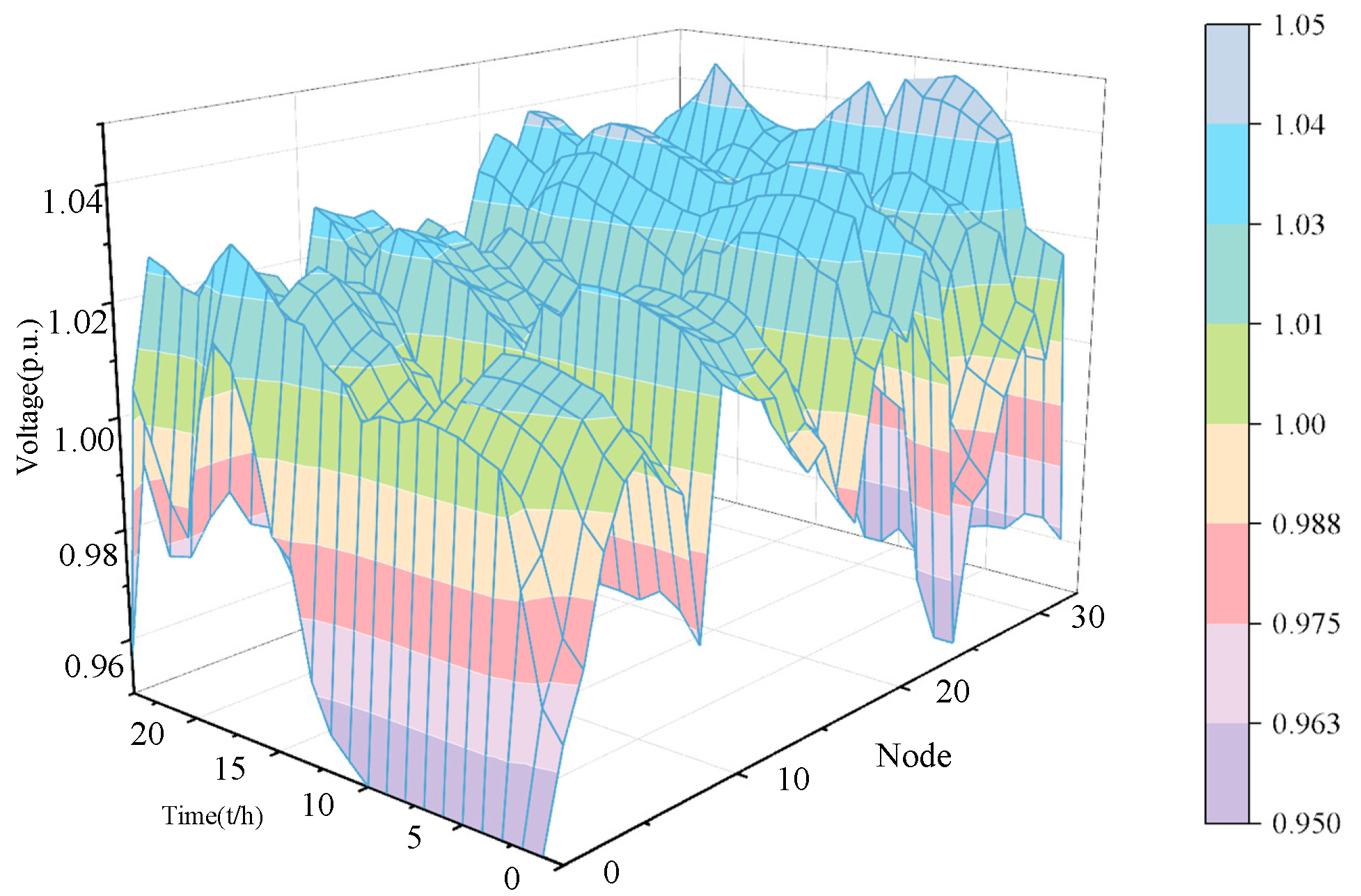
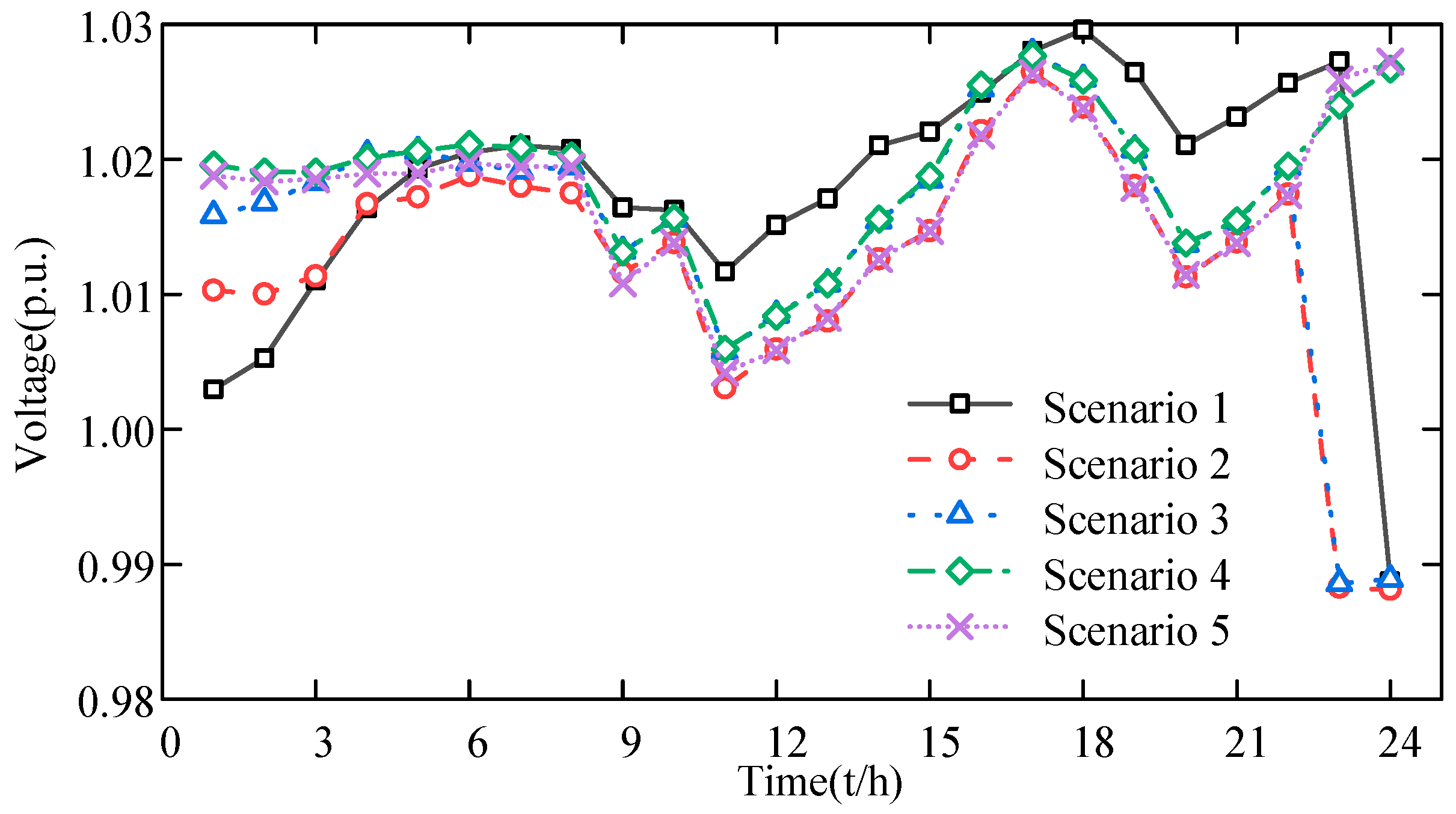
In this paper, the AC power flow model is integrated into the system framework, and the nonlinear components are handled using the second-order cone programming method. Furthermore, the influence of wind power on the system’s reactive voltage is analyzed. Simulation results demonstrate that the proposed electricity–heat–gas integrated energy system effectively reduces voltage fluctuations in the power grid and improves the overall voltage quality.
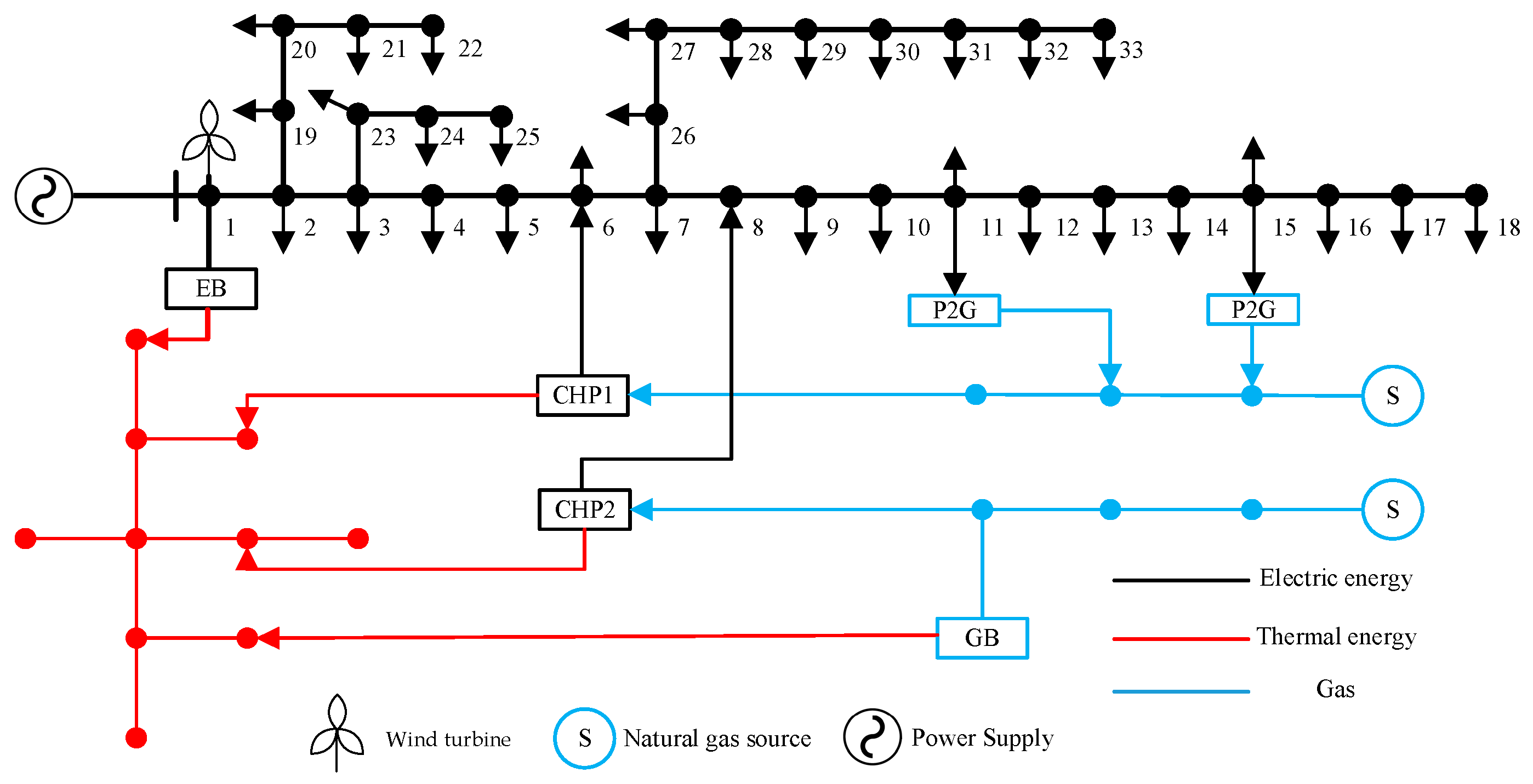
The rest of this article is organized as follows. Section 2 presents the construction of a comprehensive integrated energy system model encompassing electricity, heat, and gas. Section 3 analyzes the uncertainty of wind power output and derives a fuzzy probability distribution based on the Hausdorff distance. A two-stage distributionally robust optimization scheduling model is then developed for a virtual power plant cluster under uncertainty. Section 4 validates the effectiveness and feasibility of the proposed model through simulation results.

2. System Model

This section gives the mathematical model for the optimal scheduling of the electric heating gas integrated energy system. Based on coupling components such as cogeneration units, gas turbines, and P2G devices, establish a combined electricity–gas–heat system (CEGHS) optimization scheduling model with the goal of optimizing the overall system cost, as shown in Figure 1.

2.1. Objective Function

This model aims to minimize the total operation cost of the electricity–heat–gas system.
min C C H P + C G A S + C A W
where C C H P represents CHP unit operating cost, C G A S represents Natural gas cost, and C A W represents cost of wind abandonment.
  • Generation cost of CHP:
C C H P = i = 1 N C H P t = 1 T a i P i , t C H P 2 + b i P i , t C H P + c i + λ i s u u i , t s u + λ i s d u i , t s d
where i represents index of devices and nodes, t represents index of time periods, P i , t C H P represents the effective output of CHP unit at node i at time t , a i , b i , c i represent unit power generation cost coefficient at node i , N C H P represents the number of CHP unit, λ i s u , λ i s d represent unit startup and shutdown costs at node i , respectively, and u i s u , u i s d represent CHP unit operation status at node i .
2.
Natural gas cost:
C G A S = i = 1 N G A S λ i g a s P i , t g a s
where N G A S represents the number of gas, λ i g a s represents gas purchase cost coefficient at node i , and P i , t g a s represents gas purchase volume at node i at time t .
3.
Cost of wind abandonment:
C A W = i = 1 N W T t = 1 T κ W T P i , t p w P i , t w
where N W T represents the total number of wind turbines, κ W T represents the penalty coefficient for wind abandonment, P i , t p w represents the predicted wind power output at node i at time t , and P i , t w represents the actual wind power output at node i at time t .
The integrated energy system model of electric heating and gas set up in this paper includes the following constraints: grid constraints, heat network constraints, gas network constraints, and coupling element constraints.

2.2. Grid Constraints

  • Electric power balance constraints:
P j , t = P i , t w + P i , t C H P + P i , t e s d P i , t e s c P i , t L P i , t E B P i , t P 2 G
Q j , t = Q i , t w + Q i , t C H P + Q i , t e s d Q i , t e s c Q i , t L
where P i , t e s c , P i , t e s d represent charging and discharging active power of energy storage device at node i at time t , respectively, Q i , t e s c , Q i , t e s d represent charging and discharging reactive power of energy storage device at node i at time t , respectively, Q i , t w represents the wind reactive power output at node i at time t , Q i , t C H P represents the CHP unit reactive output at node i at time t , P i , t L , Q i , t L represent the active power and reactive power of load at node i at time t , respectively, P i , t E B represents the electric power of electric boiler at node i at time t , and P i , t P 2 G represents the P2G electrical power at node i at time t .
2.
CHP operation constraints:
u i , t C H P P i C H P min P i , t C H P u i , t C H P P i C H P max
u i , t C H P Q i C H P min Q i , t C H P u i , t C H P Q i C H P max
R i C H P P i , t C H P P i , t 1 C H P R i C H P
T i u min u i , t s u h = t t + T i u min 1 u i , t C U ,   t T T i u min + 1
T i d min u i , t s d h = t t + T i d min 1 1 u i , t C U ,   t T T i d min + 1
u i , t s u + u i , t s d 1
u i , t C U u i , t 1 C U u i , t s u u i , t s d
where P i , t C H P max , P i , t C H P min represent the upper and lower limits of unit active output at node i at time t , respectively, Q i , t C H P max , Q i , t C H P min represent the upper and lower limits of reactive power output of the unit at node i at time t , respectively, R i C H P represents the unit climbing speed at node i , u i , t C H P represents the CHP unit operation status at node i at time t , u i , t C U represents the unit that is in operation status at node i at time t , T i u min represents the minimum operating time of the unit at node i , and T i u min represents the minimum closing time of the unit at node i .
3.
Power storage device constraints:
E S t = E S t 1 + η E S C P i , t e s c 1 η E S D P i , t e s d t
E S i , 0 = 20 % E S i max
10 % E S i max E S i , t 90 % E S i max
0 P i , t e s c u i , t E S C P i E S max
0 P i , t e s d u i , t E S D P i E S max
u i , t E S C + u i , t E S D 1
where η E S C , η E S D represent the charging and discharging efficiency of energy storage devices, respectively, E S i max represents the energy storage device capacity at node i , P i , t e s c represents the CHP unit operation status at node i at time t , P i E S max represents the upper limits of electric power at node i , and u i , t E S C , u i , t E S D represent the charging and discharging status at node i at time t , respectively.
4.
Electric power restriction of electric boiler:
P i E B min P i , t E B P i E B max
where P i E B max , P i E B min represent the upper and lower limits of electric power of electric boiler at node i , respectively.
5.
Wind power output constraints:
0 P i , t w P i , t p w
6.
AC power flow constraints:
i u ( j ) ( P i j , t I i j , t 2 · r i j ) + P j , t = k v ( j ) P j k , t i u ( j ) ( Q i j , t I i j , t 2 · x i j ) + Q j , t = k v ( j ) Q j k , t I i j , t 2 = P i j , t 2 + Q i j , t 2 U i , t 2 U j , t 2 = U i , t 2 2 ( r i j · P i j , t + x i j · Q i j , t ) + ( r i j 2 + x i j 2 ) · I i j , t 2
where P i j , t , Q i j , t , I i j , t represent the active power, reactive power, and current on branch i j at time t , respectively, U i , t represents the voltage at node i at time t , and x i j , t , r i j , t represent the resistance and reactance on branch i j , respectively.
In Appendix A.1, convert the AC power flow into a second-order cone.
7.
Voltage and line power constraints:
U i min U i , t U i max
I i j min I i j , t I i j max
P i j min P i j , t P i j max
Q i j min Q i j , t Q i j max
where U i max , U i min represent the upper and lower limits of node voltage at node i , respectively, I i j max , I i j min represent the upper and lower limits of line transmission current on branch i j , respectively, P i j max , P i j min represent the upper and lower limits of active power transmission on the line on branch i j , respectively, and Q i j max , Q i j min represent the upper and lower limits of reactive power transmission on the line on branch i j , respectively.

2.3. Heat Network Constraints

The heat source, heat transfer network, and heat load constitute the heating system. The heat transfer network is divided into hydraulic and thermal models. In this paper, the heat transfer network is a hydraulic model, and the heating system’s water supply and return temperature are assumed to be constant.
  • Thermal power balance constraints:
H m , t s H m , t L + H m , t h s d H m , t h s c + n e m H m n , t = 0
H m n , t = 2 π L m n T t s T t e / R m n
H m n , t = H n m , t H n m , t , H m n , t < 0 H m n , t H m n , t c ρ v m n max S m n T t s T t r , H m n , t 0
where m , n represent the index of heating and gas network nodes, respectively, H m , t s , H m , t L represent the CHP unit thermal power and thermal load at node m at time t , respectively, H m n , t , H m n , t represent the heat network section m n power transferred and heat loss at time t , respectively, c , ρ represent the specific heat capacity and density of water, respectively, and v , S represent the medium flow rate and pipe section area, respectively.
In Appendix A.3, linearize the Heat Network Power Flow Equation.
2.
Thermal power constraints of a gas-fired boiler:
H i G B min H i , t G B H i G B max
where H i G B max , H i G B min represent the upper and lower limits of thermal power for gas boilers at node i , respectively, and H i , t G B represents the gas boiler output thermal power at node i at time t .

2.4. Gas Network Constraints

  • Natural gas source flow constraints:
G i min G i , t S G i max
where G i max , G i min represent the upper and lower limits of gas source outlet at node i , respectively, and G i , t S represents the gas source outlet at node i at time t .
2.
Node pressure constraints:
p r m , min p r m , t p r m , max
p r m , t p r n , t
where p r m , max , p r m , min represent the upper and lower limits of node air pressure at node m , respectively, and p r m , t represents the node air pressure at node m at time t .
3.
Flow equation of natural gas pipeline:
G ¯ m n , t = sgn ( p r m , t , p r n , t ) K m n g f | p r m , t 2 p r n , t 2 |
G ¯ m n , t = ( G m n , t o u t + G m n , t i n ) / 2
sgn ( p r m , t , p r n , t ) = 1 p r m , t p r n , t 1   p r m , t p r n , t
where K m , n g f represents the Weymouth constant on branch m n .
In Appendix A.2, linearize the Flow Equation of Natural Gas Pipeline.
4.
Compressor station constraints:
p r m , t Γ c p r n , t
where Γ c represents the compressor coefficient.
5.
P2G device constraints:
G i , t P 2 G = η P 2 G P i , t P 2 G
u i , t P 2 G P i , min P 2 G P i , t P 2 G u i , t P 2 G P i , max P 2 G
where η P 2 G represents the P2G hydrogen production efficiency, P i , max P 2 G , P i , min P 2 G represent the upper and lower limits of P2G electrical power at node i , respectively, and P i , t P 2 G represents the P2G electrical power at node i at time t .
6.
Network node flow balance constraints:
G n , t i n = G n , t C H P + G n , t G B + G n , t L G n , t P 2 G + G n , t g s d G n , t g s c
n G ( m ) ( G m n , t o u t G m n , t i n ) = G n , t i n
where G n , t L represents load gas consumption at node n at time t , G n , t g s d , G n , t g s c represent the outgoing and incoming volume of gas storage tanks at node n at time t , respectively, and G n , t C H P represents the CHP unit gas consumption at node n at time t .

2.5. Coupling Constraints

  • Electric boiler electrothermal coupling constraints:
H i , t E B = η E B P i , t EB
where η E B represents the heating efficiency of electric boilers.
2.
Coupling constraints of CHP:
H i , t C H P = η C H P P i , t C H P
G i , t C H P = H i , t C H P + P i , t C H P η C H P
H i CHP min H i , t CHP H i C H P max
P i , t C H P = η g p C H P G i , t C H P HHV
P i , t C H P r H H i , t CHP
where η C H P represents the CHP unit thermoelectric ratio, HHV represents the calorific value of natural gas, r H represents the gas boiler gas efficiency, and H i C H P max , H i C H P min represent the upper and lower limits of thermal power for gas boilers at node i , respectively.
3.
Gas–thermal coupling constraint of a gas-fired boiler:
P i , t G B = G i , t GB HHV
H i , t G B = η G B P i , t G B
where η G B represents the electrothermal ratio and HHV represents the calorific value of natural gas.
The optimal scheduling model of the electric heating gas integrated energy system built in this paper is complex and nonlinear, so the model is linearized as described in Section 3.

3. Data-Driven Robust Optimization Modeling Based on Hausdorff Distance

3.1. Robust Optimization Mathematical Model

The above model is represented in matrix form to create a second-order cone programming model for the optimal scheduling of the electric–thermal–gas integrated energy system:
min x , y   a T x + y T Q y + c T ξ
s . t . A x f
B x = e
C y D ξ
Q y + q 2 l T y + M
G x + H y g
J x + K y = h
The optimization variables in the model are categorized into first-stage and second-stage variables. The first stage focuses on minimizing unit operating costs and gas source costs to establish an optimal day-ahead scheduling plan, utilizing forecasts from wind power prediction scenarios. In the second stage, the CCG algorithm resolves the uncertainty probability distribution set, formulated using the Hausdorff distance, to identify the worst-case probability distribution, given the variables determined in the first stage. Please refer to Appendix B for the solution process of CCG algorithm.
Equation (53) outlines the constraints for second-stage decision variables, including the wind power forecast output vector, while Equation (54) applies second-order cone constraints to both the power and gas grids. Equations (55) and (56) detail constraints related to power, heat, and gas storage equipment, alongside the operational constraints, including startup and shutdown procedures, for conventional power units. Therefore, it can be seen from the model that the wind power output vector only exists in the objective function and (53) related to the second stage vector. This part of constraint conditions does not include the first stage variable.
Considering the discrepancies between predicted and actual wind power outputs, it is essential to comprehensively address the uncertainty of real wind power outputs in the dispatching process. Consequently, leveraging the framework established in Equations (50)–(56), a two-stage distributionally robust optimization dispatch model that accommodates wind power uncertainty is formulated as follows:
min x X , y 0 Y x , ξ 0 a T x + y 0 T Q y 0 + c T ξ 0 + max P ξ ψ E P y T Q y + c T ξ
As obtaining the probability distribution of uncertain variables in model (57) is challenging, a limited number of k discrete scenarios are selected from the n actual scenario samples to represent the potential actual output of wind power, and the corresponding initial probability distribution of the discrete scenario is obtained. This approach considers the disparity between an actual distribution and an empirical distribution. Furthermore, this paper develops a distributionally robust model that satisfies the Hausdorff distance probability constraint as follows:
min x X , y 0 Y x , ξ 0 a T x + y 0 T Q y 0 + c T ξ 0 + max P k ψ   min y k Y x , ξ k k = 1 K P k y k T Q y k + c T ξ k
The ambiguity set ψ is shown in Equation (59):
ψ = P k R + H ( P k , P k o ) θ k = 1 K P k = 1 , k = 1 , , K

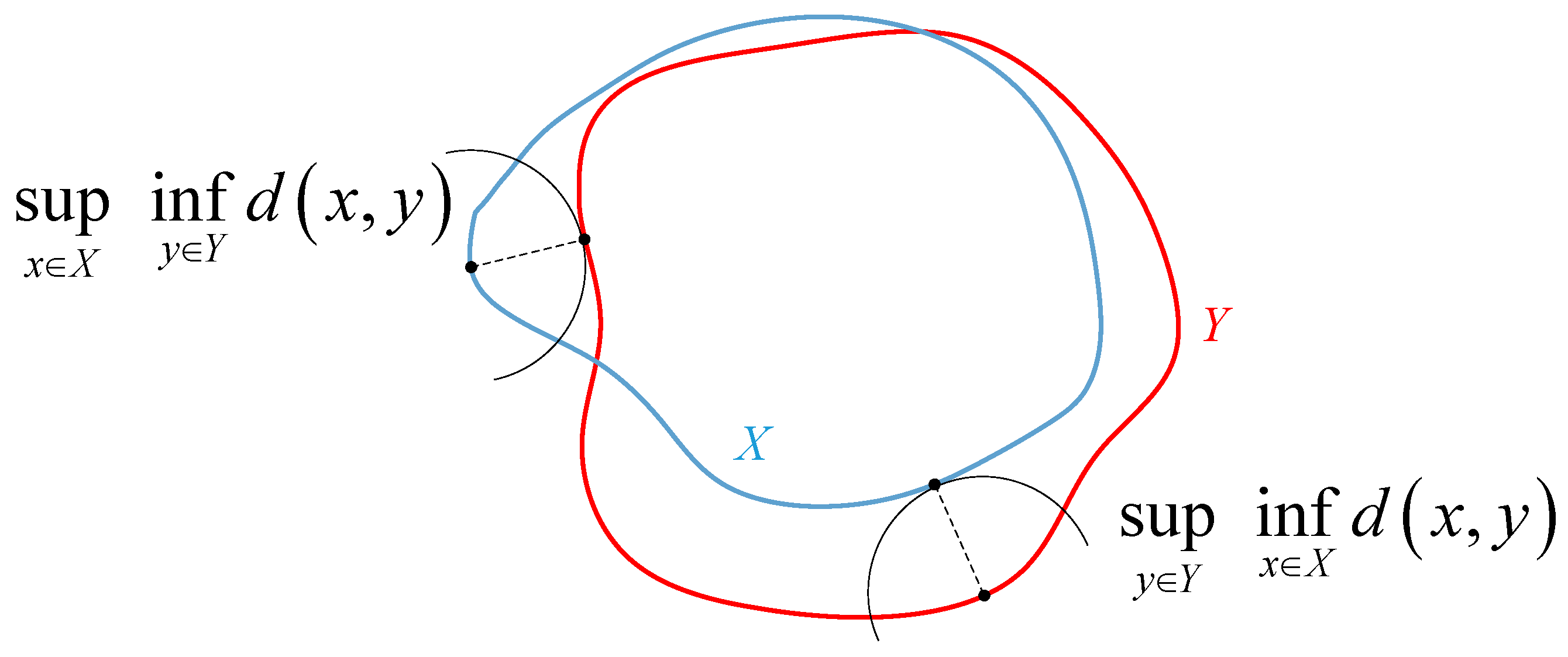
3.2. Ambiguity Set Based on Hausdorff Distance

The Hausdorff distance primarily calculates the maximum mismatch between two shapes by transforming edge feature points into two sets, thus measuring the similarity between the target and the template shapes [30]. This algorithm is applied in image recognition and biomedicine to assess the similarity of images and biomedical signals. In power system optimization, considering the uncertainty probability distribution set of wind power output is crucial. Each probability distribution value can be considered equivalent to a specific feature point of the graph, analogous to the concept of image recognition mentioned earlier. This characteristic allows it to be used for Hausdorff distance calculation. Leveraging the Hausdorff distance’s advantages in overall similarity measurement [31], this section uses it to construct the ambiguity set of uncertain variables and to assess the relationship between the overall set through a predefined ambiguity set built based on historical data. Subsequently, it comprehensively evaluates the similarity between the data-driven ambiguity set and the predefined ambiguity set.
With the increasing number of uncertain factors in power system operations in recent years, many methods have been developed to construct the uncertain probability distribution fuzzy set based on data-driven approaches.
Firstly, a fuzzy set is constructed based on distance information, including first and second-order moments. Although distance information reflects the statistical information of uncertain variables, if only distance information is used to build an uncertain probability fuzzy set, it may lead to probability distribution functions in the set that is inconsistent with reality.
The second is to build fuzzy sets based on KL divergence. Firstly, KL divergence lacks symmetry, making it unsuitable for measuring spatial distance differences between two distributions, and is primarily used to assess the information loss between them. Additionally, KL divergence requires an intersection between two probability distribution sets; without this, the results may be meaningless. Lastly, KL divergence assesses information loss at corresponding points between distributions, failing to consider their overall structure. The Hausdorff distance can measure any set in space, and there is no specific requirement for the probability distribution set. When measuring the distance between two sets, Hausdorff considers the shape and position of the two sets in the metric space and measures the overall difference.
The third is to build fuzzy sets based on Wasserstein distance. The Wasserstein distance quantifies the minimum cost of transforming one probability distribution into another, thereby measuring the distance between two distributions. Even if there is no intersection between two distribution sets, it can also be measured by the position and geometric shape of its probability distribution in space. Given that the coefficient C in the Wasserstein distance formula relates to the 1-norm, the Wasserstein distance exhibits limited anti-interference capabilities against abnormal or missing values in wind power historical data. When the collection device fails and causes the abnormal value or missing value of the collected wind power historical data, the probability distribution set under the Wasserstein distance constraint may not be effectively constrained; at the same time, the Wasserstein distance solution efficiency is affected by the size of the sample, which may lead to a long solution time. The Hausdorff distance measures the overall characteristics of two probability distributions, and the lack of a small amount of historical wind power data will not significantly impact the algorithm results. Using this feature, the outliers of some wind power data can be discarded according to the actual situation, which does not affect the calculation results of the overall distance value, and has a strong anti-interference ability for the outliers in the wind power historical data. Figure 2 illustrates the comparative analysis of Wasserstein and Hausdorff distances regarding their allowable probability deviations. The graph illustrates that with coefficient C set at 0.23, a confidence level below 0.7, and more than 50 scenarios, the permissible deviation determined using the Wasserstein distance is smaller. In contrast, under other conditions, the permissible deviation of the ambiguity set constructed using the Hausdorff distance is smaller.
The fourth is to build a fuzzy set based on norms. The norm measurement method measures the difference between the elements in the corresponding positions of two vectors and requires the measurement of the overall difference between sets. When the overall difference of the data in the set is significant, the uncertainty confidence set constrained by norms is still conservative, and its overall characteristics cannot be considered. The Hausdorff distance is a measurement method describing the similarity between two sets.
The Hausdorff distance is the distance between two compact sets in p space, which describes the maximum mismatch between the two sets. A smaller Hausdorff distance indicates a higher similarity between the two sets. The Hausdorff distance measurement method is illustrated in Figure 3.
The ambiguity set can be constructed as follows. Assuming set A = { a 1 , a 2 a p } and set B = { b 1 , b 2 b p } , the Hausdorff distance between the two sets is shown in Equation (60):
H ( A , B ) = max ( h ( A , B ) , h ( B , A ) )
h ( A , B ) = max a i A   min b j B   d ( a i , b j )
h ( B , A ) = max b j B   min a i A   d ( b j , a i )
where d ( a , b ) represents the distance between points a and b, and Euclidean distance is used in this paper.
The traditional Hausdorff distance is more sensitive to external points. An improved Hausdorff distance is given, as shown in Equations (63) and (64):
h ( A , B ) = 1 N A a i A max b j B   d ( a i , b j )
h ( B , A ) = 1 N B b i A max a j B   d ( b i , a j )
where N A and N B represent the number of points in the set. The improved Hausdorff distance uses the average value between sets to replace the maximum value between sets, which avoids the influence of some abnormal data to some extent and has good robustness. The improved Hausdorff distance can be used to derive the following confidence degree of P k :
P ( H ( A , B ) θ ) ( 1 2 N 1 e 2 θ N N 1 ) 2 N
The right side of Equation (65) is the confidence level of the uncertainty set, so the relationship between the confidence level α and the probability tolerance value θ is shown in Equation (66):
θ = N 1 2 N ln ( 2 N 1 1 a 1 / 2 N )
The relationship between the tolerance value and the confidence degree measured by considering 1-norm or infinite-norm alone is as follows according to the reference [21,30]:
θ 1 = K 2 M ln 2 K 1 2 α 1
θ = 1 2 M ln 2 K 1 2 α
It is evident from Equation (66) that as the number of historical data points increases (i.e., n), the expression gradually tends to zero. This implies that the estimated probability distribution will progressively converge to the predefined ambiguity set.
Through the comparative analysis of Equation (66) and Equations (67) and (68), it is apparent that the probability tolerance under the Hausdorff distance constraint is smaller than that under the 1-norm or -norm constraint alone. Therefore, the range of variation in the probability distribution of wind power output scenarios is correspondingly reduced.

4. Case Study

The CSECE system is selected for simulation and verification analysis in the example, including the improved IEEE-33 node, 6-node natural gas system, and 10-node thermal system. Among them, node 1 is a wind turbine, nodes 11 and 15 are coupling nodes between the power grid and the gas grid, and nodes 1, 6, and 8 are coupling nodes between the power grid and the heating network. The example was run on a desktop computer with a CPU of 2.50 GHz and a memory of 4 GB. The CPLEX solver was used to solve the problem. Figure 4 shows the system network diagram.

4.1. Analysis of Data-Driven Results Based on Hausdorff Distance

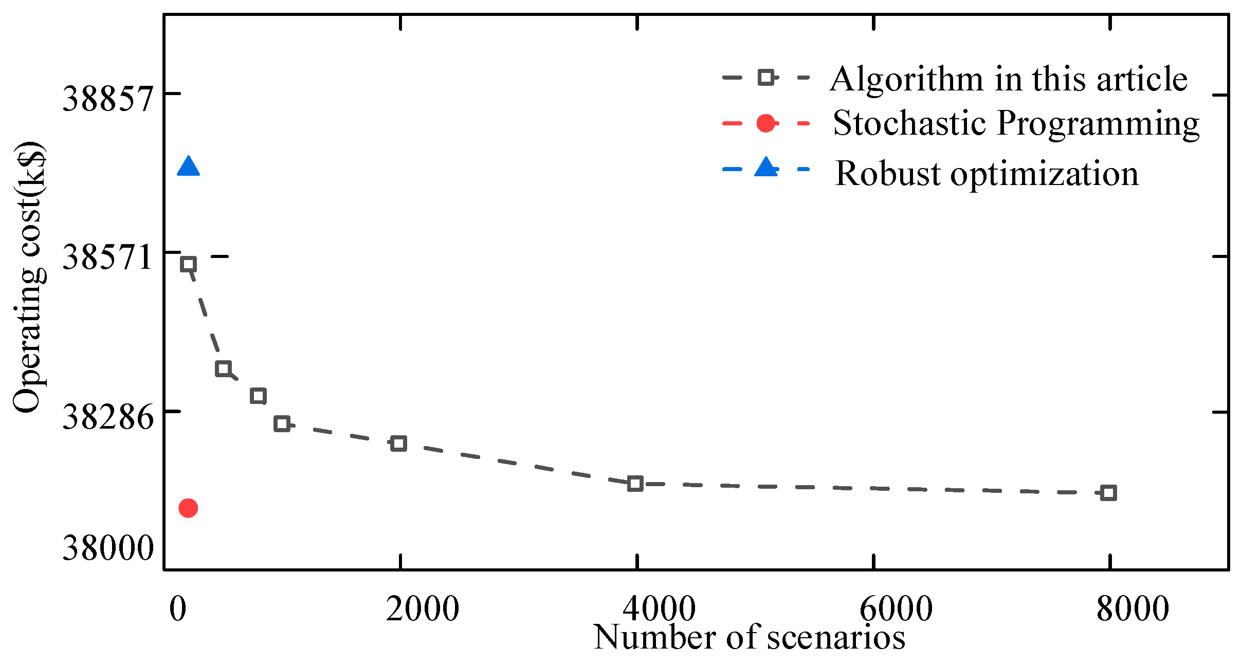
  • Economic operation cost analysis
To verify the effectiveness of the distributionally robust optimization based on Hausdorff distance data proposed in this paper, the relationship between the tolerance limit θ of the probability distribution, the confidence level α , and the total number of discrete scenarios n is obtained according to the Equation (66), as shown in Figure 5.
Additionally, a further study is conducted on the cost changes of CEGHS economic operation under different historical data numbers and confidence levels in Equation (66). The confidence level α is set to 0.5 and the typical scenario K to 2. The normal distribution is utilized to generate random scenario data representing the historical data of wind power output. The value range of wind power historical data n is [200, 8000]. Stochastic programming and robust optimization utilize the generated 8000 historical data for simulation. The results are shown in Figure 6.
It can be observed from Figure 5 and Figure 6 that as the historical data on wind power increases, the total cost of the economic operation of CEGHS decreases. This is attributed to the decrease in the tolerance value of the probability distribution function and the reduction in the ambiguity set of the actual distribution as n increases. Consequently, this diminishes the robustness of the model and gradually brings the result closer to the solution of stochastic programming.
2.
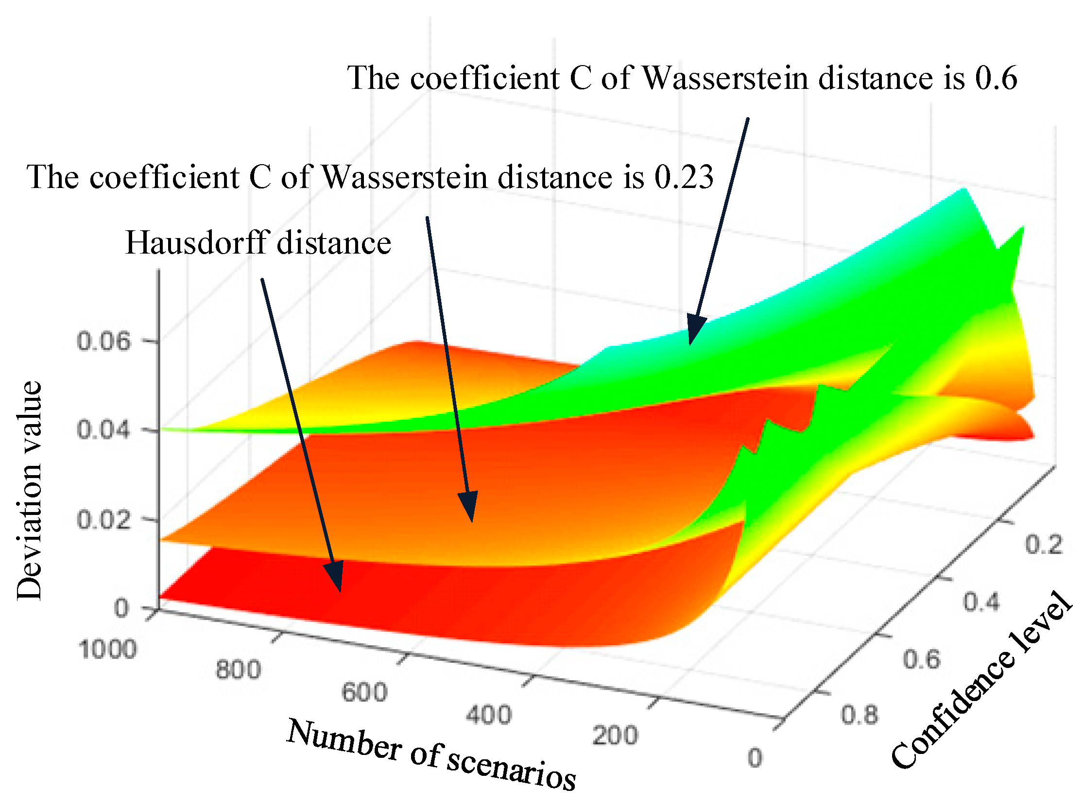
Analysis of results at various confidence levels
This section further discusses the impact of different confidence α on costs. The wind power historical data is 1000, the set number N1 is 5, the typical scenario K is 2, and the confidence α is calculated from 0.2 to 0.9.
It can be seen from Table 1 that when the number of historical data is fixed, the operating cost of CEGHS is also rising with the increase of confidence level α . This is mainly because the confidence interval increases when it becomes more extensive, and the uncertainty increases accordingly. More units are required to participate in dispatching, so the total cost of CEGHS also increases accordingly.
3.
Analysis of Hausdorff Distance and Norm Results
The results of selecting α 1 as 0.5, α as 0.9, and α as [0.2, 0.9] are shown in Table 2. It can be seen that under the Hausdorff distance constraint, the wind power output uncertainty distribution set is less conservative, and the total cost is lower than that constructed by considering the 1-norm or -norm constraints alone.

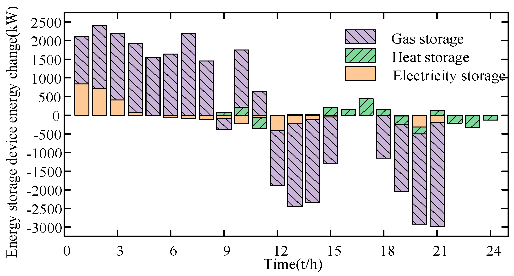
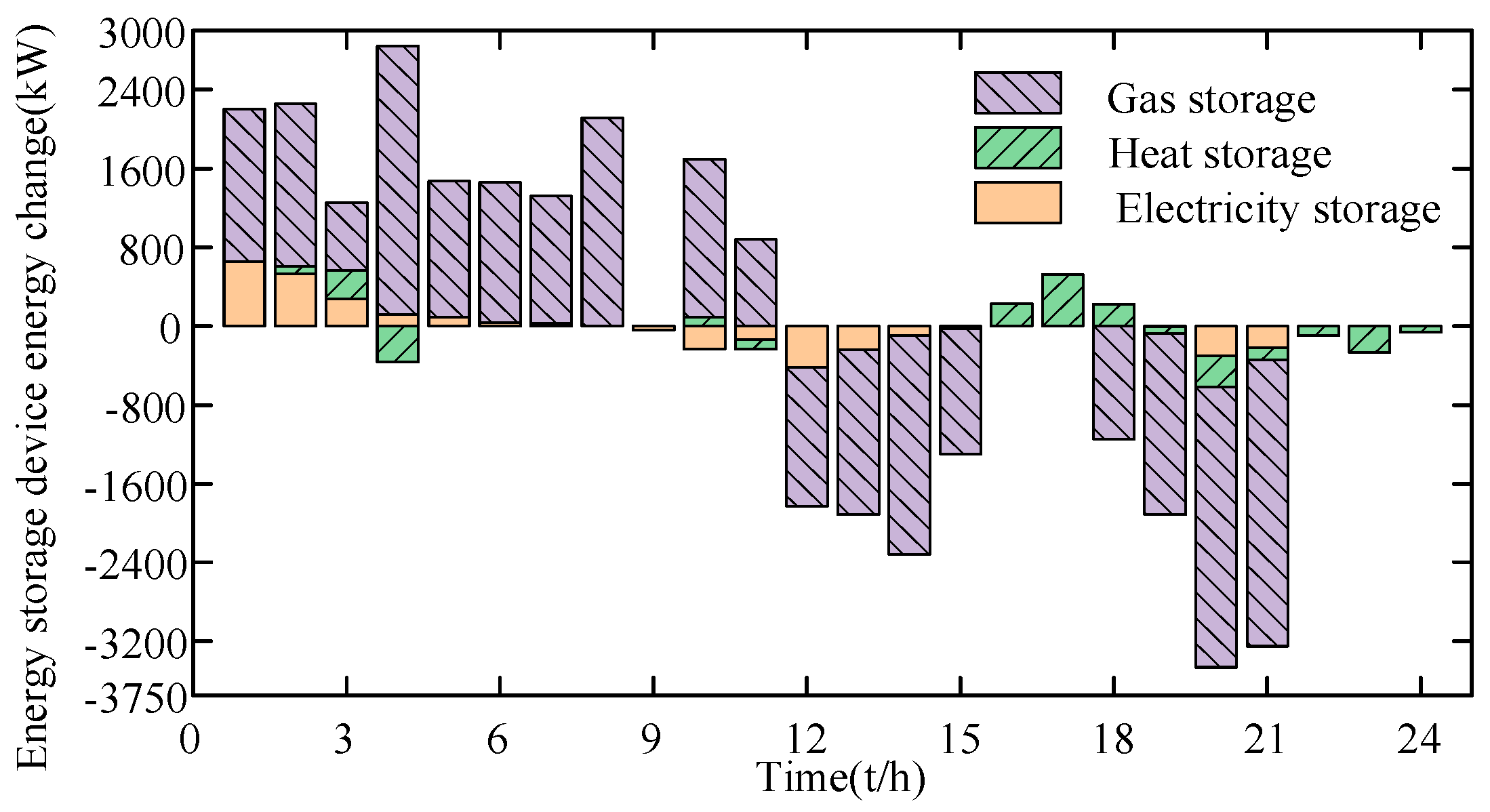
4.2. Comparative Analysis of Different Operation Scenarios of CEGHS

Five different scenarios were set for simulation analysis to verify the effectiveness of the model built in this paper.
The following validation scenarios were set:
Scenario 1: The electricity–heat–gas network operates independently and only includes the joint simulation operation of the multi-energy system of the cogeneration unit.
Scenario 2: Based on Scenario 1, power storage, gas storage, and heat storage devices are added to each network.
Scenario 3: Based on Scenario 2, coupling elements of the electric heating network are added to form the integrated energy network.
Scenario 4: Based on Scenario 2, the electrical network coupling elements are added to form the electrical integrated energy network.
Scenario 5: Based on Scenario 2, the electric, thermal, and gas coupling elements are added to form the electric-, thermal-, and gas-integrated energy network system.
  • Comparative analysis of Scenario 2 and Scenario 3
The comparative analysis between Scenario 2 and Scenario 3 examines how introducing an electricity–heating network coupling device affects the power, heating, and gas networks.
In Scenario 2, the 24 h data depicted in Figure 7 reveal that power and gas storage units accumulate energy and gas during the initial 0–3 h, while heat storage levels remain constant. This pattern suggests that the incorporation of energy storage devices enables continuous wind energy storage in the early hours. Consequently, wind energy utilization rises by 438 kWh, and the excess wind generation is cut from 1805 kWh to 1367 kWh, marking a 24.2% reduction.
Figure 8 illustrates the 24 h activity of power, gas, and heat storage devices in Scenario 3. Unlike Scenario 2, here we see that from 0–5 h, the heat storage devices not only store heat but also generate power. This contrast highlights the effect of integrating the electricity–heating network coupling device, which allows the system to convert surplus electrical energy into thermal energy. Consequently, the enhanced heat storage capability contributes to increased wind energy absorption.
2.
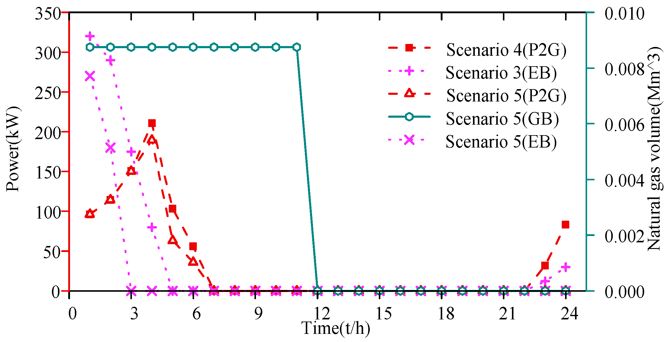
Comparative analysis of wind power output in different scenarios
In Figure 9, the integration of the electricity–heating network coupling component in Scenario 3 reduces wind power output by 1033 kWh compared to Scenario 2, marking a 21.9% decrease. A detailed view from hours 3 to 12 reveals that Scenario 3 consistently shows higher wind power output than Scenario 2, suggesting enhanced wind power absorption by the integrated network.
Comparative analysis between Scenarios 3, 4, and 5 assesses the effects of the networks operating independently versus jointly. In Scenario 5, there is a notable decrease in abandoned wind power, by 925 kWh and 405 kWh compared to Scenarios 3 and 4, resulting in reductions of 25.12% and 11.7%, respectively. It is evident that the energy output in Scenario 5 is superior to the other scenarios, indicating more efficient energy utilization.
In Figure 10, the energy consumption of each coupling component is analyzed across various scenarios. Notably, in Scenario 5, the energy output of the electric boiler shows a decrease when compared to Scenario 4. A similar reduction is observed in the power used by the P2G equipment. The green line indicates the gas consumption by the gas boiler in Scenario 5, where direct power supply to the heating network leads to fewer indirect losses from gas to electricity conversion and subsequent electric reheating. This underscores the integrated electricity–heating–gas network’s ability to achieve an economic balance among various energy forms, enhancing overall system efficiency and economic performance.
Table 3 presents a comparative analysis of the system’s optimal economic operating costs and wind power curtailment across different scenarios. The data indicate that integrating energy storage devices (Scenario 2) reduces costs compared to a base case scenario (Scenario 1), showcasing the devices’ economic benefits. Moreover, the further reduction in costs for Scenarios 3 and 4 suggests that coupling the electric–thermal and electric–gas networks enhances both the system’s economic efficiency and wind power utilization. Most notably, Scenario 5 stands out with the minimum wind power abandonment, affirming the superior performance of the integrated electricity–heat–gas system in maximizing wind energy absorption over two-network couplings.
This paper primarily compares system operating costs and wind curtailment costs under different coupling scenarios. Specifically, Scenarios 1 through 5 represent a gradual transition from a single, independently operated power grid to multiple interconnected grids. Within the integrated energy system framework, various forms of energy—electricity, heat, and gas—can complement one another, significantly enhancing overall coordination. The inclusion of energy storage devices further improves the system’s flexibility and its ability to accommodate intermittent renewable sources such as wind power. Technologies such as power-to-gas (P2G) and electric boilers enable the conversion of electricity into other energy forms, thereby reducing the output requirements—and associated costs—of gas turbines and similar units. As a result, compared to Scenario 1, Scenario 5 achieves a substantial reduction in total system cost and a marked improvement in wind power utilization efficiency.
3.
Analysis of iteration results
The confidence level A of 0.5 and the wind power historical data of 1000 were selected for algorithm analysis.
It can be seen from Table 4 that after three iterations, the model stops solving, and the calculation results are obtained, indicating that the model proposed in this paper can be solved quickly by using the CCG algorithm.

4.3. Analysis of Reactive Power and Voltage Characteristics of Electric–Heat–Gas Integrated Energy System

This section further studies and analyzes the impact of the operation of the electric–heat–gas integrated energy system proposed on the reactive voltage of the power grid.
Figure 11 illustrates the 24 h voltage profiles per unit at each node in Scenario 1. Nodes 1, 17, and 26 consistently display lower voltages, suffering significant fluctuations over the day, which suggests poor voltage quality at these points. To assess the impact of the proposed integrated energy system on node voltage distribution, a comparative analysis of voltages across all scenarios and the average voltage variation at node one has been conducted.
Figure 12 depicts the 24 h voltage fluctuations at node 1 across all scenarios. From 0 to 12 h, the consistent wind power output at node 1, coupled with insufficient reactive power compensation, results in low voltage levels. However, from 22 to 24 h, significant voltage fluctuations are observed in Scenarios 1, 2, and 3. In contrast, Scenarios 4 and 5 exhibit minimal voltage fluctuations, maintaining levels close to 1 (pu).
Figure 13 illustrates the average 24 h voltage variations across different scenarios. The analysis reveals inconsistent voltage variations across scenarios with respective ranges of 0.0409, 0.0383, 0.0392, 0.0217, and 0.023 for Scenarios 1 through 5. Figure 12 and Figure 13 demonstrate that traditional independent operation modes of energy systems tend to experience significant voltage fluctuations at both individual nodes and across the entire power grid. While the electricity–thermal coupling energy network can absorb some wind power through the heat network, it does not significantly enhance voltage stability. However, the integration of electrical coupling devices has been shown to improve overall voltage quality through resonant coupling between two independent, active sources.
The analysis highlights the effectiveness of the proposed electric–heat–gas integrated energy system in improving power grid voltage stability. Figure 11, Figure 12 and Figure 13 collectively show that traditional independent operation leads to significant voltage fluctuations, especially at critical nodes like 1, 17, and 26. Although electricity-thermal coupling networks slightly mitigate wind power impacts, they are insufficient for robust voltage control. In contrast, scenarios incorporating electrical coupling devices significantly reduce voltage variations, maintaining levels closer to 1 pu. This demonstrates that active coordination between multiple energy systems through integrated devices enhances reactive power management and overall voltage quality across the network.

5. Conclusions

This paper presents a mathematical model of an electric–heat–gas energy system, examining the impact of wind power output uncertainty on system operation.
(1)
It introduces a data-driven distributionally robust optimization method based on Hausdorff distance. This method comprehensively considers the difference between ambiguity sets and, compared with norm constraints, better simulates the true distribution of uncertainty variables. The model introduces AC power flow constraints and utilizes the second-order cone method to handle the nonlinear component. Additionally, it analyzes the impact of wind power access on system voltage quality, demonstrating that the model can reduce voltage fluctuations and enhance voltage quality.
(2)
The distributionally robust algorithm proposed in this paper strikes a better balance between economic efficiency and robustness compared to stochastic optimization and robust optimization methods. Compared to robust optimization, the proposed algorithm reduces robustness but improves economic performance. In summary, the proposed comprehensive energy system scheduling strategy outperforms traditional models in terms of economy and wind power utilization efficiency. Compared with the benchmark scenario, the operating cost of Scenario 5 has decreased by 6.65%, and the cost of wind power curtailment has decreased by 34.3%.
This study does not include other types of renewable power plants, such as solar thermal power plants. It also does not fully account for the differences in response times among various energy carriers. In addition, the study has not systematically addressed the uncertainty challenges posed by high penetration of renewable energy sources, nor has it incorporated an effective modeling framework for demand-side response mechanisms. These issues will be further explored in future research.

Author Contributions

Conceptualization, S.Z. and X.Z.; Methodology, S.Z.; Software, X.Z. and Q.C.; Validation, Q.C.; Investigation, H.Z.; Resources, H.Z.; Data curation, X.Z.; Writing—original draft, W.Z.; Visualization, W.Z. All authors have read and agreed to the published version of the manuscript.

Funding

This work was supported by the Science and Technology Project of State Grid Jiangsu Electric Power Co., Ltd. (J2024133).

Data Availability Statement

The original contributions presented in the study are included in the article, further inquiries can be directed to the corresponding author.

Conflicts of Interest

All Authors were employed by the company State Grid Jiangsu Electric Power Co., Ltd., Economic and Technical Research Institute. The remaining authors declare that the research was conducted in the absence of any commercial or financial relationships that could be construed as a potential conflict of interest.

Appendix A

Appendix A.1. Second-Order Taper of AC Power Flow

In this section, the AC power flow is converted into a mixed integer second-order cone programming (MISOCP) problem to solve [32], which is defined as follows:
X i = U i 2 , Y i j = I i j 2
Substitute the above formula into the Distflow power flow constraint of the (22) grid.
i u ( j ) ( P i j , t I i j , t 2 · r i j ) + P j , t = k v ( j ) P j k , t i u ( j ) ( Q i j , t I i j , t 2 · x i j ) + Q j , t = k v ( j ) Q j k , t I i j , t 2 = P i j , t 2 + Q i j , t 2 U i , t 2 U j , t 2 = U i , t 2 2 ( r i j · P i j , t + x i j · Q i j , t ) + ( r i j 2 + x i j 2 ) · I i j , t 2
The above power flow equation is expressed in the form of a cone function:
U i , min 2 X i U i , max 2 P l , max P i j P l , max
Y i j X I = P i j 2 + Q i j 2
Equation (A4) can be further reduced to the form of second-order cone programming:
Y i j X I P i j 2 + Q i j 2
Equation (A5) is a form that can be expressed as a rotating second-order cone, which can be converted into a second-order cone form by corresponding transformation:
  2 P i j   2 Q i j Y i j X i 2 Y i j + X i

Appendix A.2. Linearization of Flow Equation of Natural Gas Pipeline

The tidal flow equation of natural gas pipeline is a complex model integrating pressure, pipe diameter, flow, temperature, and other parameters. This paper uses the Weymouth model for research. The model is as follows:
F m n , t = sgn ( p r m , t , p r n , t ) K m n g f p r m , t 2 p r n , t 2
For non-convex nonlinearity of gas network constraints, the above formula is processed as follows [33]:
The 0–1 auxiliary variable is introduced, and the sign function is eliminated to indicate the flow direction of natural gas. Equation (34) is converted into the following form:
F m n , t 2 = ( K m n gf ) 2 ( I m n , t + I m n , t ) ( ψ m , t ψ n , t )
1 I m n , t + F m n , t max F m n , t ( 1 I m n , t ) F m n , t max
I m n , t + + I m n , t = 1
ψ m , t min ψ m , t ψ m , t max
where ψ m , t is the square of the air pressure of node m at time t. The auxiliary variable T m n is introduced to represent the pressure difference at both ends of the natural gas pipeline, and the further convex relaxation is the following second-order cone form:
T m n F m n , t 2 / ( K m n gf ) 2
T m n ψ m , t ψ n , t + ( I m n , t + + I m n , t 1 ) ( ψ m , t max ψ n , t min )
T m n ψ n , t ψ m , t + ( I m n , t + + I m n , t + 1 ) ( ψ m , t min ψ n , t max )
T m n ψ m , t ψ n , t + ( I m n , t + + I m n , t 1 ) ( ψ m , t min ψ n , t max )
T m n ψ n , t ψ m , t + ( I m n , t + + I m n , t + 1 ) ( ψ m , t max ψ n , t min )

Appendix A.3. Linearization of Heat Network Power Flow Equation

Since Equation (29) is nonlinear, 0–1 variable γ m n , t is introduced to convert Equations (27) and (29) into the following form:
n g m γ n m , t H n m , t H n m , t + 1 γ n m , t H n m , t s h m 1 γ m s , t H m s , t + H m s , t + γ m s , t H m s , t = 0
H m n , t H n m , t c ρ v m n max S m n T t s T t r
where the meaning of g ( m ) and h ( m ) is similar to that of n ( j ) and m ( j ) in the power grid; γ m n , t = 1 represents H m n , t 0 , H n m , t = 0 ; and γ m n , t = 0 stands for H m n , t = 0 , H n m , t 0 .
Since the product of 0–1 variable and thermal power is a nonlinear term, the Big-M method is used for linearization. Let ς m n , t = γ m n , t H m n , t and ς n m , t meet the following formula:
γ m n , t M ς m n , t γ m n , t M H m n , t 1 γ m n , t M ς m n , t H m n , t + 1 γ m n , t M
Equations (28), (A17), (A18), and (A19) constitute the linearized model of the heating network.

Appendix B

CCG Solving Algorithms Second-Order Taper of AC Power Flow

Equation (58) is transformed into a two-stage optimization problem, and the CCG algorithm is used to solve the model.
CCG solving algorithm
The main problem of the two-stage model is as follows:
min x X , y 0 Y x , ξ 0 , y k m Y ( x , ξ k ) , S a T x + y 0 T Q y 0 + c T ξ 0 + S
S k = 1 K P k m y k m Q y k m + c T ξ k , m = 1 , , n
Initialize probability distribution
Find the optimal solution x ,returns the lower bound of the model
Given the first stage variables x , solve the sub problem:
S x = max P k ψ k = 1 K P k   min y k Y ( x , ξ k ) y k T Q y k + c T ξ k
The model for each scenario k in the sub problem is as follows:
h x = min y k Y ( x , ξ k ) b T y k + c T ξ k
After substituting K optimal solutions h 1 , , h N s , the subproblem becomes:
S x = max P k ψ k = 1 K P k h x
The upper bound of the model obtained by solving subproblems

References

  1. Cai, Y.; Cai, J.; Xu, L.; Tan, Q.; Xu, Q. Integrated risk analysis of water-energy nexus systems based on systems dynamics, orthogonal design, and copula analysis. Renew. Sustain. Energy Rev. 2019, 99, 125–137. [Google Scholar] [CrossRef]
  2. Hu, J.; Liu, X.; Shahidehpour, M.; Xia, S. Optimal Operation of Energy Hubs with Large-Scale Distributed Energy Resources for Distribution Network Congestion Management. IEEE Trans. Sustain. Energy 2021, 12, 1755–1765. [Google Scholar] [CrossRef]
  3. Wang, D.; Liu, L.; Jia, H.; Wang, W.; Zhi, Y.; Meng, Z.; Zhou, B. Review of key problems related to integrated energy distribution systems. CSEE J. Power Energy Syst. 2018, 4, 130–145. [Google Scholar] [CrossRef]
  4. Chen, X.; Kang, C.; O’Malley, M.; Xia, Q.; Bai, J.; Liu, C.; Sun, R.; Wang, W.; Li, H. Increasing the Flexibility of Combined Heat and Power for Wind Power Integration in China: Modeling and Implications. IEEE Trans. Power Syst. 2015, 30, 1848–1857. [Google Scholar] [CrossRef]
  5. Li, J.; Fang, J.; Zeng, Q.; Chen, Z. Optimal operation of the integrated electrical and heating systems to accommodate the intermittent renewable sources. Appl. Energy 2016, 167, 244–254. [Google Scholar] [CrossRef]
  6. Li, Z.; Wu, W.; Wang, J.; Zhang, B.; Zheng, T. Transmission-Constrained Unit Commitment Considering Combined Electricity and District Heating Networks. IEEE Trans. Sustain. Energy 2016, 7, 480–492. [Google Scholar] [CrossRef]
  7. Vandewalle, J.; Bruninx, K.; D’Haeseleer, W. Effects of large-scale power to gas conversion on the power, gas and carbon sectors and their interactions. Energy Convers. Manag. 2015, 94, 28–39. [Google Scholar] [CrossRef]
  8. Zhang, X.; Shahidehpour, M.; Alabdulwahab, A.; Abusorrah, A. Optimal Expansion Planning of Energy Hub with Multiple Energy Infrastructures. IEEE Trans. Smart Grid 2015, 6, 2302–2311. [Google Scholar] [CrossRef]
  9. Götz, M.; Lefebvre, J.; Mörs, F.; Koch, A.M.; Graf, F.; Bajohr, S.; Reimert, R.; Kolb, T. Renewable power-to-gas: A technological and economic review. Renew. Energy 2016, 85, 1371–1390. [Google Scholar] [CrossRef]
  10. Salimi, M.; Ghasemi, H.; Adelpour, M.; Vaez-Zadeh, S. Optimal planning of energy hubs in interconnected energy systems: A case study for natural gas and electricity. Gener. Transm. Distrib. Iet 2015, 9, 695–707. [Google Scholar] [CrossRef]
  11. Qadrdan, M.; Wu, J.; Jenkins, N.; Ekanayake, J. Operating Strategies for a GB Integrated Gas and Electricity Network Considering the Uncertainty in Wind Power Forecasts. IEEE Trans. Sustain. Energy 2014, 5, 128–138. [Google Scholar] [CrossRef]
  12. Alabdulwahab, A.; Abusorrah, A.; Zhang, X.; Shahidehpour, M. Coordination of Interdependent Natural Gas and Electricity Infrastructures for firming the Variability of Wind Energy in Stochastic Day-Ahead Scheduling. IEEE Trans. Sustain. Energy 2015, 6, 606–615. [Google Scholar] [CrossRef]
  13. Li, Y.; Zou, Y.; Tan, Y.; Cao, Y.; Liu, X.; Shahidehpour, M.; Tian, S.; Bu, F. Optimal Stochastic Operation of Integrated Low-Carbon Electric Power, Natural Gas, and Heat Delivery System. IEEE Trans. Sustain. Energy 2018, 9, 273–283. [Google Scholar] [CrossRef]
  14. He, C.; Wu, L.; Liu, T.; Shahidehpour, M. Robust Co-Optimization Scheduling of Electricity and Natural Gas Systems via ADMM. IEEE Trans. Sustain. Energy 2017, 8, 658–670. [Google Scholar] [CrossRef]
  15. Zhang, Y.; Ai, X.; Wen, J.; Fang, J.; He, H. Data-Adaptive Robust Optimization Method for the Economic Dispatch of Active Distribution Networks. IEEE Trans. Smart Grid 2019, 10, 3791–3800. [Google Scholar] [CrossRef]
  16. Duan, C.; Fang, W.; Jiang, L.; Yao, L.; Liu, J. Distributionally Robust Chance-Constrained Approximate AC-OPF with Wasserstein Metric. IEEE Trans. Power Syst. 2018, 33, 4924–4936. [Google Scholar] [CrossRef]
  17. Lu, X.; Chan, K.W.; Xia, S.; Zhou, B.; Luo, X. Security-Constrained Multiperiod Economic Dispatch with Renewable Energy Utilizing Distributionally Robust Optimization. IEEE Trans. Sustain. Energy 2019, 10, 768–779. [Google Scholar] [CrossRef]
  18. Shi, Z.; Liang, H.; Huang, S.; Dinavahi, V. Distributionally Robust Chance-Constrained Energy Management for Islanded Microgrids. IEEE Trans. Smart Grid 2019, 10, 2234–2244. [Google Scholar] [CrossRef]
  19. Ding, Y.; Morstyn, T.; McCulloch, M.D. Distributionally Robust Joint Chance-Constrained Optimization for Networked Microgrids Considering Contingencies and Renewable Uncertainty. IEEE Trans. Smart Grid 2022, 13, 2467–2478. [Google Scholar] [CrossRef]
  20. Duan, C.; Jiang, L.; Fang, W.; Liu, J.; Liu, S. Data-Driven Distributionally Robust Energy-Reserve-Storage Dispatch. IEEE Trans. Ind. Inform. 2018, 14, 2826–2836. [Google Scholar] [CrossRef]
  21. Xiong, P.; Jirutitijaroen, P.; Singh, C. A Distributionally Robust Optimization Model for Unit Commitment Considering Uncertain Wind Power Generation. IEEE Trans. Power Syst. 2017, 32, 39–49. [Google Scholar] [CrossRef]
  22. Alismail, F.; Xiong, P.; Singh, C. Optimal Wind Farm Allocation in Multi-Area Power Systems Using Distributionally Robust Optimization Approach. IEEE Trans. Power Syst. 2018, 33, 536–544. [Google Scholar] [CrossRef]
  23. Chen, Y.; Guo, Q.; Sun, H.; Li, Z.; Wu, W.; Li, Z. A Distributionally Robust Optimization Model for Unit Commitment Based on Kullback–Leibler Divergence. IEEE Trans. Power Syst. 2018, 33, 5147–5160. [Google Scholar] [CrossRef]
  24. Hu, Z.; Hong, J.L. Kullback–Leibler Divergence Constrained Distributionally Robust Optimization. 2012. Available online: http://www.optimization-online.org/DB_FILE/2012/11/3677.pdf (accessed on 15 March 2024).
  25. Wang, C.; Gao, R.; Wei, W.; Shafie-khah, M.; Bi, T.; Catalão, J.P.S. Risk-Based Distributionally Robust Optimal Gas-Power Flow with Wasserstein Distance. IEEE Trans. Power Syst. 2019, 34, 2190–2204. [Google Scholar] [CrossRef]
  26. Zhao, P.; Gu, C.; Cao, Z.; Hu, Z.; Zhang, X.; Chen, X.; Hernando-Gil, I.; Ding, Y. Economic-Effective Multi-Energy Management Considering Voltage Regulation Networked with Energy Hubs. IEEE Trans. Power Syst. 2021, 36, 2503–2515. [Google Scholar] [CrossRef]
  27. Ding, T.; Yang, Q.; Yang, Y.; Li, C.; Bie, Z.; Blaabjerg, F. A Data-Driven Stochastic Reactive Power Optimization Considering Uncertainties in Active Distribution Networks and Decomposition Method. IEEE Trans. Smart Grid 2018, 9, 4994–5004. [Google Scholar] [CrossRef]
  28. Zhao, C.; Guan, Y. Data-Driven Stochastic Unit Commitment for Integrating Wind Generation. IEEE Trans. Power Syst. 2016, 31, 2587–2596. [Google Scholar] [CrossRef]
  29. Zeng, B.; Zhao, L. Solving two-stage robust optimization problems using a column-and-constraint generation method. Oper. Res. Lett. 2013, 41, 457–461. [Google Scholar] [CrossRef]
  30. Taha, A.; Allan, H. An efficient algorithm for calculating the exact Hausdorff distance. IEEE Trans. Pattern Anal. Mach. Intell. 2015, 37, 2153–2163. [Google Scholar] [CrossRef]
  31. Schutze, O.; Esquivel, X.; Lara, A.; Coello, C.A.C. Using the averaged Hausdorff distance as a performance measure in evolutionary multiobjective optimization. IEEE Trans. Evol. Comput. 2012, 16, 504–522. [Google Scholar] [CrossRef]
  32. Farivar, M.; Low, S.H. Branch Flow Model: Relaxations and Convexification—Part II. IEEE Trans. Power Syst. 2013, 28, 2565–2572. [Google Scholar] [CrossRef]
  33. He, Y.; Yan, M.; Shahidehpour, M.; Li, Z.; Guo, C.; Wu, L.; Ding, Y. Decentralized Optimization of Multi-Area Electricity-Natural Gas Flows Based on Cone Reformulation. IEEE Trans. Power Syst. 2018, 33, 4531–4542. [Google Scholar] [CrossRef]
Figure 1. Combined electricity–gas–heat system.
Energies 18 02442 g001
Figure 2. Comparison of allowable deviation values between Wasserstein distance and Hausdorff distance.
Energies 18 02442 g002
Figure 3. Hausdorff distance.
Energies 18 02442 g003
Figure 4. CEGHS network diagram.
Energies 18 02442 g004
Figure 5. Error distribution based on Hausdorff distance.
Energies 18 02442 g005
Figure 6. Results under different scenarios were compared and analyzed.
Energies 18 02442 g006
Figure 7. Output of each energy storage device in Scenario 2.
Energies 18 02442 g007
Figure 8. Output of each energy storage device in Scenario 3.
Energies 18 02442 g008
Figure 9. Comparison diagram of wind power output in various scenarios.
Energies 18 02442 g009
Figure 10. Schematic diagram of coupling element output.
Energies 18 02442 g010
Figure 11. Node voltage distribution diagram of Scenario 1.
Energies 18 02442 g011
Figure 12. Voltage variation diagram of each scenario’s node 1.
Energies 18 02442 g012
Figure 13. Overall mean voltage variation diagram for each scenario.
Energies 18 02442 g013
Table 1. Results were compared and analyzed under different confidence levels.
Confidence Level a Model Economic Operating Cost (kUSD)
0.237,913
0.538,261
0.738,289
0.938,309
Table 2. Comparison of Hausdorff distance with 1-norm and -norm results.
Confidence
Level a
Model Economic Operating Cost (kUSD)
Hausdorff Distance1-Norm -Norm
0.237,91338,30938,299
0.538,26138,30938,299
0.738,28938,30938,299
0.938,31038,30938,299
Table 3. Operating cost of each scenario and wind abandonment.
Scenario12345
Operating Cost (kUSD)40,98740,22038,79938,86638,261
Cost of wind
abandonment (kUSD)
548.4438.1395.1401.1360.6
Table 4. Iterative solution results.
IterationsUpper Bound Value (kUSD)Lower Bound Value (kUSD)
162,66422,399
23866937,847
338,26138,261
Disclaimer/Publisher’s Note: The statements, opinions and data contained in all publications are solely those of the individual author(s) and contributor(s) and not of MDPI and/or the editor(s). MDPI and/or the editor(s) disclaim responsibility for any injury to people or property resulting from any ideas, methods, instructions or products referred to in the content.

